Evidence for Nonlinear Isotope Shift in Yb⁺ Search for New Boson

Abstract

We measure isotope shifts for five Yb⁺ isotopes with zero nuclear spin on two narrow optical quadrupole transitions ${}^{2}S_{1/2}\rightarrow{}^{2}D_{3/2}$, ${}^{2}S_{1/2}\rightarrow{}^{2}D_{5/2}$ with an accuracy of $\sim 300$ Hz. The corresponding King plot shows a $3\times 10^{-7}$ deviation from linearity at the 3 $\sigma$ uncertainty level. Such a nonlinearity can indicate physics beyond the Standard Model (SM) in the form of a new bosonic force carrier, or arise from higher-order nuclear effects within the SM. We identify the quadratic field shift as a possible nuclear contributor to the nonlinearity at the observed scale, and show how the nonlinearity pattern can be used in future, more accurate measurements to separate a new-boson signal from nuclear effects.

The Standard Model (SM) of particle physics describes virtually all measurements of elementary particles exquisitely well, and yet various indirect evidence points to physics beyond the SM. This evidence includes the preponderance of dark matter of unknown composition in our Universe, astronomically observed with several different methodologies such as the rotation curves of galaxies [1], the motion of colliding galaxy clusters [2], gravitational lensing [3], and the power spectrum of the cosmic microwave background [4]. Physics beyond the SM is also being probed in various laboratory experiments, such as high-energy collisions [5], searches for weakly interacting massive particles [5], axions, and axionlike particles [6], precision measurements of the electric dipole moments of elementary particles [7], and other precision tests [8].

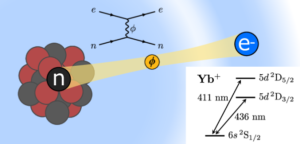
Figure 1: New intra-atomic force between electron ($e^{-}$) and neutron ($n$) mediated by the virtual exchange of a hypothetical new boson $\phi$. The coupling results in a Yukawa-like potential that modifies the atomic energy levels and can be probed with isotope-shift spectroscopy. We perform precision measurements of the long-lived states ${}^{2}D_{3/2}$, ${}^{2}D_{5/2}$ on individual trapped Yb⁺ ions.

Dark-matter candidates can be characterized by their mass, spin, and interactions. In the intermediate mass range from $\sim 100$ eV$/c^{2}$ to $\sim 100$ MeV$/c^{2}$, a new method has been proposed to search for a dark-matter boson $\phi$ that couples to quarks and leptons [9, 10]. The virtual exchange of $\phi$ between neutrons and electrons in an atom would result in a Yukawa-like potential in addition to the Coulomb potential of the nucleus (see Fig. 1). The corresponding shift in energy levels and transition frequencies is too small to be detected by directly comparing spectroscopic data to (much less accurate) atomic-structure calculations, but could potentially be detected through precision isotope-shift measurements [11, 12, 13, 14] that allow one to sidestep electronic-structure calculations. In particular, the scaled isotope shifts on two different transitions exhibit a linear relationship (King plot [15]), and Refs. [9, 10] argue that a deviation from linearity can indicate a new force mediator $\phi$. Such studies are particularly timely as recent experiments analyzing nuclear decay in ⁸Be and ⁴He have observed a 7 $\sigma$ deviation from the SM [16, 17, 18] that could be potentially explained by a new boson with a mass of 17 MeV/$c^{2}$ ($X17$ boson) [19, 20, 21, 22]. According to Ref. [10], measurements of optical transitions with a resolution of 1 Hz in select atomic systems could probe this scenario. However, higher-order effects within the SM can result in nonlinearities that limit the sensitivity to new physics [23, 24, 25, 26].

In this Letter, we report a precision measurement of the isotope shift for five isotopes of Yb⁺ ions with zero nuclear spin on two narrow optical quadrupole transitions (${}^{2}S_{1/2}\rightarrow{}^{2}D_{3/2},{}^{2}D_{5/2}$) with an accuracy of $\sim 300$ Hz. Displaying the data in a King plot [15], we observe a deviation from linearity at the $10^{-7}$ level, corresponding to 3 standard deviations $\sigma$. With four independent isotope-shift data points available, we further introduce a novel parametrization of the nonlinearity pattern that can be used to distinguish between nonlinearities of the same magnitude but different physical origin. At the current level of precision, the observed nonlinearity pattern is consistent with both a new boson, and the quadratic field shift (QFS) [23] that we identify as the leading source of nonlinearity within the SM by means of precision electronic-structure calculations. In the future, more accurate measurements on the present and other optical transitions in Yb and Yb⁺ [27, 28, 29] can discriminate between effects within and outside the SM.

Table 1: Inverse-mass differences $\mu_{ji}$ and measured isotope shifts $\nu_{ji}$ between next-neighboring pairs of five even Yb⁺ isotopes. $\mu_{ji}$ is calculated from the mass of Yb⁺ ions with the ionization energy set to 6.254 eV [30, 31, 32]. The nuclear size difference $\delta\langle{r^{2}}\rangle$ is deduced from $\nu_{ji}$ using the calculated parameters $F_{\alpha}^{\mathrm{CI}}=-15.852$ GHz/fm², $F_{\beta}^{\mathrm{CI}}=-16.094$ GHz/fm², $F_{\alpha}^{\mathrm{MBPT}}=-16.570$ GHz/fm², $F_{\beta}^{\mathrm{MBPT}}=-16.771$ GHz/fm², $K_{\alpha}^{\mathrm{CI}}=-1678.3~{}\mathrm{GHz\cdot u}$, and $K_{\beta}^{\mathrm{CI}}=-1638.5~{}\mathrm{GHz\cdot u}$ (see the Supplemental Material [33]). The uncertainties given here and throughout the paper for $\nu_{\alpha ji}$ and $\nu_{\beta ji}$ indicate 1$\sigma$ statistical uncertainties; the estimated systematic uncertainties on these quantities are $<20$% of the statistical uncertainties (see the Supplemental Material [33]). The (170,174) pair is directly measured as a cross-check [the measurements (170,174) and (170,172), (172,174) agree within 2 $\sigma$] and to improve precision (see the Supplemental Material [33]). In the calculations of $\delta\langle{r^{2}}\rangle_{ji}$ from the measured isotope shifts, the average of the values for $\alpha$ and $\beta$ is given (the difference between transitions is less than 0.2%) (see the Supplemental Material [33]), and the values of $K_{\alpha}$ and $K_{\beta}$ from the CI calculations are used for both CI and MBPT. For the data from Ref. [34] (last column), only the statistical errors are presented in the parentheses, while the systematic errors from the calculation of the electronic factors are much larger.

Isotope pair	$\mu_{ji}$ ($10^{-6}\mathrm{u}^{-1}$)	$\nu_{\alpha ji}$ (kHz)	$\nu_{\beta ji}$ (kHz)	$\delta\langle{r^{2}}\rangle_{ji}$ (fm2)
$(j,i)$		$\alpha:{}^{2}S_{1/2}\rightarrow{}^{2}D_{5/2}$	$\beta:{}^{2}S_{1/2}\rightarrow{}^{2}D_{3/2}$	CI	MBPT	Reference [34]
(168, 170)	70.113 698(46)	2 179 098.93(21)	2 212 391.85(37)	-0.156	-0.149	-0.1561(3)
(170, 172)	68.506 890 50(63)	2 044 854.78(34)	2 076 421.58(39)	-0.146	-0.140	-0.1479(1)
(172, 174)	66.958 651 95(64)	1 583 068.42(36)	1 609 181.47(22)	-0.115	-0.110	-0.1207(1)
(174, 176)	65.474 078 21(65)	1 509 055.29(28)	1 534 144.06(24)	-0.110	-0.105	-0.1159(1)
(170, 174)		3 627 922.95(50)	3 685 601.95(33)

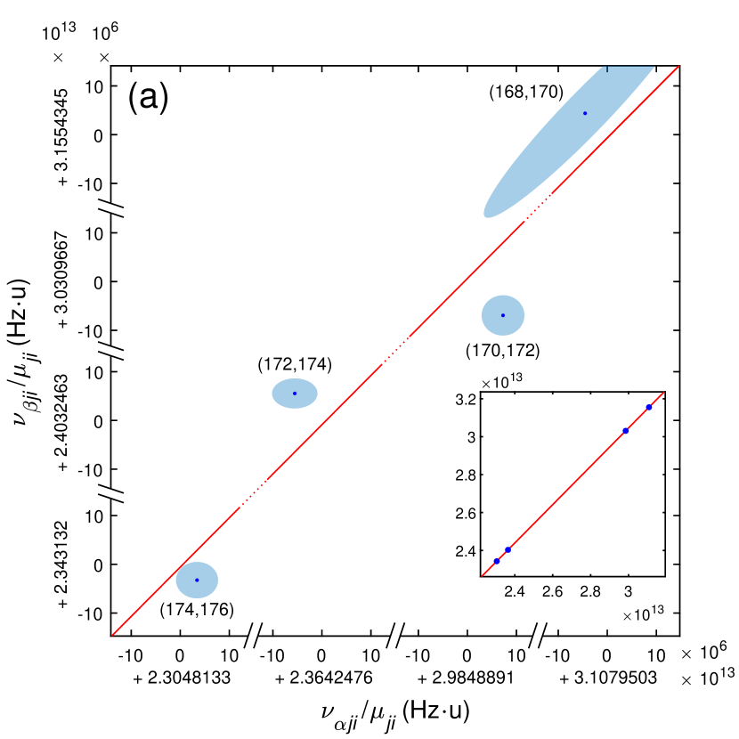
Figure 2: (a) Standard King plot [Eq. (2)] for the $\alpha=411$ nm, ${}^{2}S_{1/2}\rightarrow{}^{2}D_{5/2}$, and $\beta=436$ nm, ${}^{2}S_{1/2}\rightarrow{}^{2}D_{3/2}$ transitions for pairs of neighboring even Yb$+$ isotopes. The inset shows the full King plot. The main figure is zoomed into the data points by a factor of $10^{6}$. A deviation from linearity (red line) by 3 standard deviations $\sigma$ is observed. The larger diagonal uncertainty for the $(168,170)$ pair is due to the larger mass uncertainty for the ¹⁶⁸Yb⁺ isotope [30, 31, 32] (see the Supplemental Material [33]). (b) Frequency-normalized King plot [Eq. (3)] and residuals. The error bars and error ellipses indicate $1\sigma$.

Our measurements are performed with individual ${}^{j}\text{Yb}^{+}$ ions ($j\in\{168,170,172,174,176\}$) trapped in a linear Paul trap, and Doppler cooled on the $6s\,{}^{2}S_{1/2}\rightarrow 6p\,{}^{2}P_{1/2}$ transition to typically 500 $\mu$K [35]. We perform optical precision spectroscopy on the transitions to two long-lived excited states (with electron configurations $[\text{Xe}]4f^{14}6s\,{}^{2}S_{1/2}\rightarrow[\text{Xe}]4f^{14}5d\,{}^{2}D_{3/2},{}^{2}D_{5/2}$) using light at the wavelengths 411 and 436 nm, respectively. The probe light is generated by a frequency-doubled Ti:Sapphire laser that is frequency stabilized to an ultralow-thermal-expansion cavity, achieving a short-term stability of $\sim 200$ Hz. Typically, 1 mW of 411-nm light (0.2 mW of 436-nm light) is focused to a waist of $w_{0}=60~{}\mathrm{\mu m}$ ($w_{0}=15~{}\mathrm{\mu m}$) at the location of the ion (see Supplemental Material (the Supplemental Material) [33] for details).

Coherent optical Ramsey spectroscopy is carried out with two $\frac{\pi}{2}$ pulses of 411- or 436-nm light, lasting 5 $\mu$s each, separated by 10 $\mu$s. This is followed by readout of the state, performed using an electron-shelving scheme [36] (see the Supplemental Material [33]). A small magnetic field of typically $\sim 1.1$ G is applied to separate the different Zeeman components of the $S\rightarrow D$ transition. Frequency scans are taken over the central Ramsey fringes of the two symmetric Zeeman components with the lowest magnetic-field sensitivity to find the center frequency of the transition (see the Supplemental Material [33]).

The measurement on one isotope is averaged typically for 30 minutes before we switch to a next-neighboring isotope by adjusting various loading, cooling, and repumper laser frequencies. We typically perform three interleaved measurements of each isotope to determine an isotope shift, allowing us to reach a precision on the order of $\sim 300$ Hz (see Table 1 and Fig. 2), limited mainly by drifts in the frequency stabilization of the probe laser to the ultrastable cavity (see the Supplemental Material [33]).

The frequency shift $\nu_{\alpha ji}$ between isotope ^jYb and ⁱYb on an optical transition $\alpha$ can be written as a sum of terms that factorize into a nuclear part (with subscript $ji$) and an electronic part (with subscript $\alpha$) [15, 24, 9]

$$\nu_{\alpha ji}=F_{\alpha}\delta\langle{r^{2}}\rangle_{ji}+K_{\alpha}\mu_{ji}+G_{\alpha}[\delta\langle{r^{2}}\rangle^{2}]_{ji}+\upsilon_{ne}D_{\alpha}a_{ji}$$ (1)

Here $\delta\langle{r^{2}}\rangle_{ji}\equiv\langle{r^{2}}\rangle_{j}-\langle{r^{2}}\rangle_{i}$ is the difference in squared charge radii $r$ between isotope $j$ and $i$, $\mu_{ji}\equiv 1/m_{j}-1/m_{i}$ is the inverse-mass difference, $[\delta\langle{r^{2}}\rangle^{2}]_{ji}\equiv(\delta\langle{r^{2}}\rangle_{jl})^{2}-(\delta\langle{r^{2}}\rangle_{il})^{2}$ for some fixed isotope $l$ (the choice of $l$ is irrelevant to the nonlinearity) (see the Supplemental Material [33]), and $a_{ji}=j-i$ is the difference in neutron number. The quantity $\upsilon_{ne}=(-1)^{s+1}y_{n}y_{e}/(4\pi\hbar c)$ is the product of the coupling factors of the new boson to the neutron $y_{n}$ and electron $y_{e}$, creating a Yukawa-like potential given by $V_{ne}(r)=\hbar c\,\upsilon_{ne}\exp(-r/\lambdabar_{c})/r$ for a boson with spin $s$, mass $m_{\phi}$, and reduced Compton wavelength $\lambdabar_{c}=\hbar/(m_{\phi}c)$ [24, 9].

For heavy elements like Yb, the first term in Eq. (1) associated with the change in nuclear size $\delta\langle{r^{2}}\rangle$ [“field shift” (FS)] dominates, while the second term is due to the electron’s reduced mass and momentum correlations between electrons (“mass shift”). According to our electronic-structure calculations (see below), the third (QFS) term associated with the square of nuclear size $[\delta\langle{r^{2}}\rangle^{2}]_{ji}$ represents the leading-order nonlinearity [24, 23] within the SM for Yb. The last term describes the isotope shift due to the Yukawa-like potential associated with the new boson $\phi$. The quantities $F,K,G,D$ are determined by the electronic wave functions of the transition [9, 10, 24]; see the Supplemental Material [33]. Note that the effect of the next-leading order Seltzer moment [37, 24] associated with $\delta\langle{r^{4}}\rangle$ is absorbed into the QFS term; see the Supplemental Material [33].

The first two terms in Eq. (1) lead to a linear relationship between the isotope shifts (King plot [15]) when one considers two different transitions $\alpha,\beta$,

$$\overline{\overline{\nu}}_{\beta ji}=K_{\beta\alpha}+F_{\beta\alpha}\overline{\overline{\nu}}_{\alpha ji}+G_{\beta\alpha}\overline{\overline{[\delta\langle{r^{2}}\rangle^{2}]}}_{ji}+\upsilon_{ne}D_{\beta\alpha}\overline{\overline{a}}_{ji}$$ (2)

Here we define $F_{\beta\alpha}\equiv F_{\beta}/F_{\alpha}$, $P_{\beta\alpha}\equiv P_{\beta}-F_{\beta\alpha}P_{\alpha}$ for $P\in\{K,G,D\}$, while $\overline{\overline{z}}_{ji}\equiv z_{ji}/\mu_{ji}$ for $z\in\{\nu_{\alpha},\nu_{\beta,},[\delta\langle{r^{2}}\rangle^{2}],a\}$, is the inverse-mass-normalized quantity. For our purposes, where the FS dominates, the influence of mass and frequency errors is more transparent if we instead write a modified linear relationship for the frequency-normalized quantities $\overline{x}_{ji}\equiv x_{ji}/\nu_{\alpha ji}$ for $x\in\{\nu_{\beta},\mu,[\delta\langle{r^{2}}\rangle^{2}],a\}$

$$\overline{\nu}_{\beta ji}=F_{\beta\alpha}+K_{\beta\alpha}\overline{\mu}_{ji}+G_{\beta\alpha}\overline{[\delta\langle{r^{2}}\rangle^{2}]}_{ji}+\upsilon_{ne}D_{\beta\alpha}\overline{a}_{ji}$$ (3)

To analyze the experimental results in this work, the transitions and isotopes are assigned as follows: $\alpha={}^{2}S_{1/2}\rightarrow{}^{2}D_{5/2}$ (411 nm), $\beta={}^{2}S_{1/2}\rightarrow{}^{2}D_{3/2}$ (436 nm), $j\in\{168,170,172,174\}$ with $i=j+2$, and $l=172$.

The inset in Fig. 2(a) confirms the general linear relationship for the inverse-mass-normalized isotope shifts in a standard King plot corresponding to Eq. (2) for the two transitions $\alpha$ and $\beta$. However, when we zoom in by a factor of $10^{6}$ [main figure 2(a)], we observe a small deviation from linearity, in the range 0.5 – 1 kHz in frequency units for a given data point. The frequency-normalized King plot associated with Eq. (3), as displayed in Fig. 2(b), illustrates that due to the smallness of the slope, i.e. the mass-shift electronic factor $K_{\beta\alpha}$, the mass error along the horizontal axis $\overline{\mu}_{ji}$ has a negligible effect. For all points taken together, the nonlinearity is nonzero at the level of 3 $\sigma$ (see the Supplemental Material [33]).

With four independent isotope pairs, we can quantify not only the magnitude of the nonlinearity, but also an associated pattern further characterizing the nonlinearity. To this end, we introduce two dimensionless nonlinearity measures

$$\zeta_{\pm}\equiv d_{168}-d_{170}\pm(d_{172}-d_{174})$$ (4)

where $d_{j}\equiv\overline{\nu}_{\beta ji}-f(\overline{\mu}_{ji})$ are the vertical deviations of the four data points $\overline{\nu}_{\beta ji}$ in Fig. 2(b) from the linear fit $f$. $\zeta_{+}$ and $\zeta_{-}$ characterize the two possible nonlinearities for four data points, a zigzag shape with deviation pattern $+-+-$, and a curved nonlinearity with deviation pattern $+--+$, respectively. Any given nonlinearity can be represented by a point in the $\zeta_{+}\zeta_{-}$ plane [see Fig. 3(a)]. A nonlinearity that arises from the coupling of the $\phi$ boson to the neutron number corresponds to a fixed nonlinearity pattern, and hence a given line through the origin (see the Supplemental Material [33]). The same argument holds for the QFS. Our observed nonlinearity lies close to both lines representing pure coupling to a new boson and the QFS, respectively. The experimental uncertainty region in Fig. 3(a) can be decomposed into its possible QFS and new-boson components, as shown in Fig. 3(b). It highlights the relative contributions of the two sources of nonlinearity, ranging from pure new boson to pure QFS contribution at the current level of uncertainty. With increased measurement precision, it will be possible to separate the two contributions.

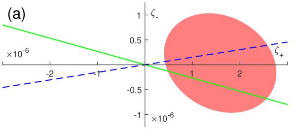
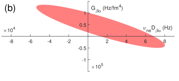
Figure 3: (a) Nonlinearity measure $(\zeta_{+},\zeta_{-})$ for next-neighbor isotope pairs. The red shaded region indicates the 95% confidence interval from our data. The green solid line and the blue dashed line indicate the required ratio $\zeta_{-}/\zeta_{+}$ if the nonlinearity is purely due to a new boson $\phi$ and the QFS, respectively. (b) Experimental nonlinearity measure along the axes of a new boson ($x$-axis) and the QFS ($y$-axis).

In order to convert the observed nonlinearity, as represented by $\zeta_{\pm}$, into a physical quantity such as the coupling $\upsilon_{ne}$, we need to determine the associated electronic wave functions. To cross-check our numerical simulations for systematic errors, we use two different methods, the Dirac-Hartree-Fock method [38, 39] followed by the configuration interaction (CI) method [40, 41, 42, 43], using the software package GRASP2018 [44], and many-body perturbation theory (MBPT) [45] implemented in ambit [46]. We calculate $F_{\beta\alpha}^{\mathrm{CI}}=1.0153$ and $F_{\beta\alpha}^{\mathrm{MBPT}}=1.0121$, within 0.2% and 0.07% of our experimental value $F_{\beta\alpha}^{\mathrm{exp}}=1.01141024(86)$, respectively. For the mass shift, that is more difficult to calculate accurately, we find $K_{\beta\alpha}^{\mathrm{CI}}=65~{}\mathrm{GHz\cdot u}$ (see the Supplemental Material [33]), within a factor of 2 from the experimental value $K_{\beta\alpha}^{\mathrm{exp}}=120.208(23)~{}\mathrm{GHz\cdot u}$. The calculated wave functions in combination with the measured frequency shift can also be used to extract the nuclear size difference $\delta\langle{r^{2}}\rangle$ (see the Supplemental Material [33]), in good agreement with other results [34]; see Table 1. We also calculate $G_{\beta\alpha}^{\mathrm{CI}}=232$ kHz/fm⁴ and $G_{\beta\alpha}^{\mathrm{MBPT}}=-36$ kHz/fm⁴ for the QFS, indicating a large systematic uncertainty in the calculation of this small term. The experimentally constrained range in Fig. 3(b) (24 – 94 kHz/fm⁴) (see the Supplemental Material [33]) lies between the two calculated values.

Using the electronic-structure calculations, we can determine a boundary on the new-boson coupling from our data. Figure 4 shows the upper bound on the product of couplings $|y_{e}y_{n}|$. It is obtained by dividing the experimental value of $\upsilon_{ne}D_{\beta\alpha}$ from Fig. 3(b) (determined with the assumption that the effect of the new boson dominates the nonlinearity; i.e., $G_{\beta\alpha}=0$), by $(-1)^{s+1}D_{\beta\alpha}(m_{\phi})/(4\pi\hbar c)$ from the atomic-structure calculations (see the Supplemental Material [33] for the calculation of $D_{\beta\alpha}$). The calculations with the CI and the MBPT methods agree with each other to better than a factor of 2 over most of the mass range $m_{\phi}$. The upper bound from our data on $|y_{e}y_{n}|$ is $\sim 200$ times larger than the preferred coupling range for the $X17$ boson [19, 20], and 2 orders of magnitude larger than the bound estimated in Ref. [10] from the combination of $g-2$ measurements on the electron and neutron scattering data. We note, however, that the limit on $|y_{e}|$ depends on additional assumptions about the new boson’s spin and the symmetries of the interaction.

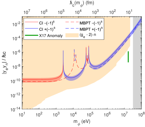
Figure 4: Product of couplings $\left|y_{e}y_{n}\right|$ of a new boson vs. boson mass $m_{\phi}$ (bottom) and reduced Compton wavelength (top), plotted under the assumption that the observed nonlinearity in Fig. 3 is dominated by the new boson. The solid line is for the CI calculation, and the dashed line is for the MBPT calculation. If the nonlinearity has a contribution from the QFS, then $\left|y_{e}y_{n}\right|$ lies below this line. The gray shade indicates the region inside the nucleus. The sign of $y_{e}y_{n}$ is color-coded: red for $-(-1)^{s}$ and blue for $+(-1)^{s}$ for a spin-$s$ boson. The 95% confidence intervals from the statistical uncertainty in the measured isotope shift are shown as shaded areas along the solid line. The systematic uncertainty due to the wave function calculation is much larger, especially in the high-mass region. The thick green line indicates the preferred coupling range for the $X17$ boson from the Be/He anomaly [16, 17, 18, 19, 20, 21]. The yellow shaded area shows the constraint from electron $g_{e}-2$ measurements [47, 48, 49, 50, 51] combined with neutron scattering measurements [52, 53, 54, 55] (from Ref. [10]).

Finally, since the absolute optical frequency of the ${}^{2}S_{1/2}\rightarrow{}^{2}D_{5/2}$ transition for ¹⁷²Yb⁺ has recently been measured with precision at the Hz level [56], the absolute frequencies for all the other bosonic isotopes can be deduced from our isotope shift measurements. The results are summarized in Table 2.

Table 2: Frequencies of the ${}^{2}S_{1/2}\rightarrow{}^{2}D_{5/2}$ transition.

Isotope	Absolute frequency (kHz)	Ref.
168	729 481 090 980.86(36)	This work
170	729 478 911 881.93(30)	This work
172	729 476 867 027.2068(44)	[56]
174	729 475 283 958.85(31)	This work
176	729 473 774 903.56(42)	This work

In the future, the measurement precision can be increased by several orders of magnitude by cotrapping two isotopes [12, 13]. This improvement, also in combination with measurements on additional transitions, such as the ${}^{2}S_{1/2}\rightarrow{}^{2}F_{7/2}$ octupole transition in Yb⁺ [57] or clock transitions in neutral Yb [28, 29], will allow one to discriminate between nonlinearities of different origin. Characterizing the nonlinearities arising from within the SM can provide new information about the nucleus [58], especially in combination with improved electronic-structure calculations. On the other hand, if evidence for a new boson should emerge from the improved measurements, it can be independently verified by performing similar measurements on other atomic species [10], such as Ca/Ca⁺ [59, 13, 60], Sr/Sr⁺ [14, 12], Nd⁺ [61], or on highly charged ions [62, 63, 64, 65], as well as on molecules like Sr₂ [66]. Unstable isotopes (e.g. ¹⁶⁶Yb with a half-life of $\sim 2.4$ days) can be used to increase the number of points in the King Plot, providing strong further constraints on the origin of the nonlinearity. The generalization of nonlinearity measures $\zeta_{\pm}$ for more isotopes or transitions is discussed in the Supplemental Material [33].

This work was supported by the NSF and NSF CUA. This project received funding from the European Union’s Horizon 2020 research and innovation programme under the Marie Sklodowska-Curie Grant No. 795121. C.L. was supported by the U. S. Department of Defense (DoD) through the National Defense Science & Engineering Graduate Fellowship (NDSEG) Program. J.C.B. is supported by the Australian Research Council (DP190100974). A.K. acknowledges the partial support of a William M. and Jane D. Fairbank Postdoctoral Fellowship of Stanford University. We thank M. Drewsen, V. V. Flambaum, P. Harris, N. Huntemann, T. Mehlstäubler, R. Milner, R. Ozeri, E. Peik, G. Perez, R.F. Garcia Ruiz, Y. Soreq, J. Thaler, and T. Zelevinsky for interesting discussions, W. Nazarewicz and P. Reinhard for providing information about the Yb nucleus, and V. Dzuba for pointing out the nuclear quadrupole deformation as a potential significant source of nonlinearity [26].

References

- Rubin et al. [1980] V. C. Rubin, W. K. Ford, and N. Thonnard, Astrophys. J. 238, 471 (1980), URL http://adsbit.harvard.edu//full/1980ApJ...238..471R/0000471.000.html.
- Clowe et al. [2006] D. Clowe, M. Bradač, A. H. Gonzalez, M. Markevitch, S. W. Randall, C. Jones, and D. Zaritsky, The Astrophysical Journal 648, L109 (2006), URL https://doi.org/10.1086%2F508162.
- Massey et al. [2010] R. Massey, T. Kitching, and J. Richard, Reports on Progress in Physics 73, 086901 (2010), URL https://doi.org/10.1088%2F0034-4885%2F73%2F8%2F086901.
- Akrami et al. [2018] Y. Akrami et al. (Planck Collaboration) (2018), eprint arXiv:1807.06205, URL https://arxiv.org/abs/1807.06205.
- Tanabashi et al. [2018] M. Tanabashi et al. (Particle Data Group), Phys. Rev. D 98, 030001 (2018), URL https://link.aps.org/doi/10.1103/PhysRevD.98.030001.
- Graham et al. [2015] P. W. Graham, I. G. Irastorza, S. K. Lamoreaux, A. Lindner, and K. A. van Bibber, Annual Review of Nuclear and Particle Science 65, 485 (2015), eprint https://doi.org/10.1146/annurev-nucl-102014-022120, URL https://doi.org/10.1146/annurev-nucl-102014-022120.
- Chupp et al. [2019] T. E. Chupp, P. Fierlinger, M. J. Ramsey-Musolf, and J. T. Singh, Rev. Mod. Phys. 91, 015001 (2019), URL https://link.aps.org/doi/10.1103/RevModPhys.91.015001.
- Safronova et al. [2018a] M. S. Safronova, D. Budker, D. DeMille, D. F. J. Kimball, A. Derevianko, and C. W. Clark, Rev. Mod. Phys. 90, 025008 (2018a), URL https://link.aps.org/doi/10.1103/RevModPhys.90.025008.
- Delaunay et al. [2017] C. Delaunay, R. Ozeri, G. Perez, and Y. Soreq, Phys. Rev. D 96, 093001 (2017), URL https://link.aps.org/doi/10.1103/PhysRevD.96.093001.
- Berengut et al. [2018] J. C. Berengut, D. Budker, C. Delaunay, V. V. Flambaum, C. Frugiuele, E. Fuchs, C. Grojean, R. Harnik, R. Ozeri, G. Perez, et al., Phys. Rev. Lett. 120, 091801 (2018), URL https://link.aps.org/doi/10.1103/PhysRevLett.120.091801.
- Gebert et al. [2015] F. Gebert, Y. Wan, F. Wolf, C. N. Angstmann, J. C. Berengut, and P. O. Schmidt, Phys. Rev. Lett. 115, 053003 (2015), URL https://link.aps.org/doi/10.1103/PhysRevLett.115.053003.
- Manovitz et al. [2019] T. Manovitz, R. Shaniv, Y. Shapira, R. Ozeri, and N. Akerman, Phys. Rev. Lett. 123, 203001 (2019), URL https://link.aps.org/doi/10.1103/PhysRevLett.123.203001.
- Knollmann et al. [2019] F. W. Knollmann, A. N. Patel, and S. C. Doret, Phys. Rev. A 100, 022514 (2019), URL https://link.aps.org/doi/10.1103/PhysRevA.100.022514.
- Miyake et al. [2019] H. Miyake, N. C. Pisenti, P. K. Elgee, A. Sitaram, and G. K. Campbell, Phys. Rev. Research 1, 033113 (2019), URL https://link.aps.org/doi/10.1103/PhysRevResearch.1.033113.
- King [1984] W. H. King, Isotope Shifts in Atomic Spectra (Plenum Press, New York, 1984).
- Krasznahorkay et al. [2018] A. J. Krasznahorkay, M. Csatlós, L. Csige, Z. Gácsi, J. Gulyás, Á. Nagy, N. Sas, J. Timár, T. G. Tornyi, I. Vajda, et al., Journal of Physics: Conference Series 1056, 012028 (2018), ISSN 1742-6588, URL http://stacks.iop.org/1742-6596/1056/i=1/a=012028?key=crossref.10a8b6db295a5c09f5d12be531be382e.
- Krasznahorkay et al. [2016] A. J. Krasznahorkay, M. Csatlós, L. Csige, Z. Gácsi, J. Gulyás, M. Hunyadi, I. Kuti, B. M. Nyakó, L. Stuhl, J. Timár, et al., Phys. Rev. Lett. 116, 042501 (2016), URL https://link.aps.org/doi/10.1103/PhysRevLett.116.042501.
- Krasznahorkay et al. [2019] A. J. Krasznahorkay, M. Csatlos, L. Csige, J. Gulyas, M. Koszta, B. Szihalmi, J. Timar, D. S. Firak, A. Nagy, N. J. Sas, et al. (2019), eprint 1910.10459.
- Feng et al. [2016] J. L. Feng, B. Fornal, I. Galon, S. Gardner, J. Smolinsky, T. M. P. Tait, and P. Tanedo, Phys. Rev. Lett. 117, 071803 (2016), URL https://link.aps.org/doi/10.1103/PhysRevLett.117.071803.
- Feng et al. [2017] J. L. Feng, B. Fornal, I. Galon, S. Gardner, J. Smolinsky, T. M. P. Tait, and P. Tanedo, Phys. Rev. D 95, 035017 (2017), URL https://link.aps.org/doi/10.1103/PhysRevD.95.035017.
- Jentschura and Nándori [2018] U. D. Jentschura and I. Nándori, Phys. Rev. A 97, 042502 (2018), URL https://link.aps.org/doi/10.1103/PhysRevA.97.042502.
- Banerjee et al. [2018] D. Banerjee, V. E. Burtsev, A. G. Chumakov, D. Cooke, P. Crivelli, E. Depero, A. V. Dermenev, S. V. Donskov, R. R. Dusaev, T. Enik, et al. (NA64 Collaboration), Phys. Rev. Lett. 120, 231802 (2018), URL https://link.aps.org/doi/10.1103/PhysRevLett.120.231802.
- Flambaum et al. [2018] V. V. Flambaum, A. J. Geddes, and A. V. Viatkina, Phys. Rev. A 97, 032510 (2018), URL https://link.aps.org/doi/10.1103/PhysRevA.97.032510.
- Mikami et al. [2017] K. Mikami, M. Tanaka, and Y. Yamamoto, The European Physical Journal C 77, 896 (2017), ISSN 1434-6052, URL https://doi.org/10.1140/epjc/s10052-017-5467-4.
- Tanaka and Yamamoto [2019] M. Tanaka and Y. Yamamoto (2019), eprint 1911.05345.
- Allehabi et al. [2020] S. O. Allehabi, V. A. Dzuba, V. V. Flambaum, A. V. Afanasjev, and S. E. Agbemava (2020), eprint 2001.09422.
- Huntemann et al. [2016] N. Huntemann, C. Sanner, B. Lipphardt, C. Tamm, and E. Peik, Phys. Rev. Lett. 116, 063001 (2016), URL https://link.aps.org/doi/10.1103/PhysRevLett.116.063001.
- Barber et al. [2006] Z. W. Barber, C. W. Hoyt, C. W. Oates, L. Hollberg, A. V. Taichenachev, and V. I. Yudin, Phys. Rev. Lett. 96, 083002 (2006), URL https://link.aps.org/doi/10.1103/PhysRevLett.96.083002.
- Safronova et al. [2018b] M. S. Safronova, S. G. Porsev, C. Sanner, and J. Ye, Phys. Rev. Lett. 120, 173001 (2018b), URL https://link.aps.org/doi/10.1103/PhysRevLett.120.173001.
- Huang et al. [2017] W. Huang, G. Audi, M. Wang, F. G. Kondev, S. Naimi, and X. Xu, Chinese Physics C 41, 030002 (2017), URL https://doi.org/10.1088%2F1674-1137%2F41%2F3%2F030002.
- Wang et al. [2017] M. Wang, G. Audi, F. G. Kondev, W. Huang, S. Naimi, and X. Xu, Chinese Physics C 41, 030003 (2017), URL https://doi.org/10.1088%2F1674-1137%2F41%2F3%2F030003.
- Rana et al. [2012] R. Rana, M. Höcker, and E. G. Myers, Phys. Rev. A 86, 050502(R) (2012), URL https://link.aps.org/doi/10.1103/PhysRevA.86.050502.
- [33] See Supplemental Material for the details on experimental protocols, data analysis, estimation of systematic effects, and the calculation of electronic state-dependent factors.
- Angeli and Marinova [2013] I. Angeli and K. Marinova, Atomic Data and Nuclear Data Tables 99, 69 (2013), ISSN 0092-640X, URL http://www.sciencedirect.com/science/article/pii/S0092640X12000265.
- Cetina et al. [2013] M. Cetina, A. Bylinskii, L. Karpa, D. Gangloff, K. M. Beck, Y. Ge, M. Scholz, A. T. Grier, I. Chuang, and V. Vuletić, New Journal of Physics 15, 053001 (2013), URL https://doi.org/10.1088%2F1367-2630%2F15%2F5%2F053001.
- Taylor et al. [1997] P. Taylor, M. Roberts, S. V. Gateva-Kostova, R. B. M. Clarke, G. P. Barwood, W. R. C. Rowley, and P. Gill, Phys. Rev. A 56, 2699 (1997), URL https://link.aps.org/doi/10.1103/PhysRevA.56.2699.
- Seltzer [1969] E. C. Seltzer, Phys. Rev. 188, 1916 (1969), URL https://link.aps.org/doi/10.1103/PhysRev.188.1916.
- Grant et al. [1980] I. Grant, B. McKenzie, P. Norrington, D. Mayers, and N. Pyper, Computer Physics Communications 21, 207 (1980), ISSN 0010-4655, URL http://www.sciencedirect.com/science/article/pii/0010465580900417.
- Dyall et al. [1989] K. Dyall, I. Grant, C. Johnson, F. Parpia, and E. Plummer, Computer Physics Communications 55, 425 (1989), ISSN 0010-4655, URL http://www.sciencedirect.com/science/article/pii/0010465589901367.
- Jönsson et al. [1996] P. Jönsson, A. Ynnerman, C. Froese Fischer, M. R. Godefroid, and J. Olsen, Phys. Rev. A 53, 4021 (1996), URL https://link.aps.org/doi/10.1103/PhysRevA.53.4021.
- Porsev et al. [2009] S. G. Porsev, M. G. Kozlov, and D. Reimers, Phys. Rev. A 79, 032519 (2009), URL https://link.aps.org/doi/10.1103/PhysRevA.79.032519.
- Fawcett and Wilson [1991] B. Fawcett and M. Wilson, Atomic Data and Nuclear Data Tables 47, 241 (1991), ISSN 0092-640X, URL http://www.sciencedirect.com/science/article/pii/0092640X9190003M.
- Biémont et al. [1998] E. Biémont, J.-F. Dutrieux, I. Martin, and P. Quinet, Journal of Physics B 31, 3321 (1998), URL https://doi.org/10.1088%2F0953-4075%2F31%2F15%2F006.
- Froese Fischer et al. [2019] C. Froese Fischer, G. Gaigalas, P. Jönsson, and J. Bieroń, Computer Physics Communications 237, 184 (2019), ISSN 0010-4655, URL http://www.sciencedirect.com/science/article/pii/S0010465518303928.
- Dzuba et al. [1985] V. A. Dzuba, V. V. Flambaum, P. G. Silvestrov, and O. P. Sushkov, Journal of Physics B: Atomic and Molecular Physics 18, 597 (1985), URL https://doi.org/10.1088%2F0022-3700%2F18%2F4%2F008.
- Kahl and Berengut [2019] E. Kahl and J. Berengut, Computer Physics Communications 238, 232 (2019), ISSN 0010-4655, URL http://www.sciencedirect.com/science/article/pii/S0010465518304302.
- Hanneke et al. [2008] D. Hanneke, S. Fogwell, and G. Gabrielse, Phys. Rev. Lett. 100, 120801 (2008), URL https://link.aps.org/doi/10.1103/PhysRevLett.100.120801.
- Hanneke et al. [2011] D. Hanneke, S. Fogwell Hoogerheide, and G. Gabrielse, Phys. Rev. A 83, 052122 (2011), URL https://link.aps.org/doi/10.1103/PhysRevA.83.052122.
- Aoyama et al. [2012] T. Aoyama, M. Hayakawa, T. Kinoshita, and M. Nio, Phys. Rev. Lett. 109, 111807 (2012), URL https://link.aps.org/doi/10.1103/PhysRevLett.109.111807.
- Bouchendira et al. [2011] R. Bouchendira, P. Cladé, S. Guellati-Khélifa, F. Nez, and F. Biraben, Phys. Rev. Lett. 106, 080801 (2011), URL https://link.aps.org/doi/10.1103/PhysRevLett.106.080801.
- Davoudiasl et al. [2014] H. Davoudiasl, H.-S. Lee, and W. J. Marciano, Phys. Rev. D 89, 095006 (2014), URL https://link.aps.org/doi/10.1103/PhysRevD.89.095006.
- Barbieri and Ericson [1975] R. Barbieri and T. Ericson, Physics Letters 57B, 270 (1975), ISSN 0370-2693, URL http://www.sciencedirect.com/science/article/pii/0370269375900738.
- Leeb and Schmiedmayer [1992] H. Leeb and J. Schmiedmayer, Phys. Rev. Lett. 68, 1472 (1992), URL https://link.aps.org/doi/10.1103/PhysRevLett.68.1472.
- Pokotilovski [2006] Y. N. Pokotilovski, Physics of Atomic Nuclei 69, 924 (2006), URL https://doi.org/10.1134/S1063778806060020.
- Nesvizhevsky et al. [2008] V. V. Nesvizhevsky, G. Pignol, and K. V. Protasov, Phys. Rev. D 77, 034020 (2008), URL https://link.aps.org/doi/10.1103/PhysRevD.77.034020.
- Fürst et al. [2020] H. A. Fürst, C.-H. Yeh, D. Kalincev, A. P. Kulosa, L. S. Dreissen, R. Lange, E. Benkler, N. Huntemann, E. Peik, and T. E. Mehlstäubler (2020), eprint 2006.14356.
- Roberts et al. [1997] M. Roberts, P. Taylor, G. P. Barwood, P. Gill, H. A. Klein, and W. R. C. Rowley, Phys. Rev. Lett. 78, 1876 (1997), URL https://link.aps.org/doi/10.1103/PhysRevLett.78.1876.
- Reinhard et al. [2020] P.-G. Reinhard, W. Nazarewicz, and R. F. Garcia Ruiz, Phys. Rev. C 101, 021301(R) (2020), URL https://link.aps.org/doi/10.1103/PhysRevC.101.021301.
- Solaro et al. [2020] C. Solaro, S. Meyer, K. Fisher, J. C. Berengut, E. Fuchs, and M. Drewsen, Phys. Rev. Lett. 125, 123003 (2020), URL https://link.aps.org/doi/10.1103/PhysRevLett.125.123003.
- Mortensen et al. [2004] A. Mortensen, J. J. T. Lindballe, I. S. Jensen, P. Staanum, D. Voigt, and M. Drewsen, Phys. Rev. A 69, 042502 (2004), URL https://link.aps.org/doi/10.1103/PhysRevA.69.042502.
- Bhatt et al. [2020] N. Bhatt, K. Kato, and A. C. Vutha (2020), eprint 2002.08290.
- Micke et al. [2020] P. Micke, T. Leopold, S. A. King, E. Benkler, L. J. Spieß, L. Schmöger, M. Schwarz, J. R. Crespo López-Urrutia, and P. O. Schmidt, Nature (London) 578, 60 (2020), ISSN 0028-0836, URL http://dx.doi.org/10.1038/s41586-020-1959-8http://www.nature.com/articles/s41586-020-1959-8.
- Yerokhin et al. [2020] V. A. Yerokhin, R. A. Müller, A. Surzhykov, P. Micke, and P. O. Schmidt, Phys. Rev. A 101, 012502 (2020), URL https://link.aps.org/doi/10.1103/PhysRevA.101.012502.
- Silwal et al. [2018] R. Silwal, A. Lapierre, J. D. Gillaspy, J. M. Dreiling, S. A. Blundell, Dipti, A. Borovik, G. Gwinner, A. C. C. Villari, Y. Ralchenko, et al., Phys. Rev. A 98, 052502 (2018), URL https://link.aps.org/doi/10.1103/PhysRevA.98.052502.
- Kozlov et al. [2018] M. G. Kozlov, M. S. Safronova, J. R. Crespo López-Urrutia, and P. O. Schmidt, Rev. Mod. Phys. 90, 045005 (2018), URL https://link.aps.org/doi/10.1103/RevModPhys.90.045005.
- McGuyer et al. [2015] B. H. McGuyer, M. McDonald, G. Z. Iwata, M. G. Tarallo, A. T. Grier, F. Apfelbeck, and T. Zelevinsky, New Journal of Physics 17, 055004 (2015), URL https://doi.org/10.1088%2F1367-2630%2F17%2F5%2F055004.