TTP-2020-016, P3H-20-014
A Study of New Physics Searches with Tritium and Similar Molecules

Abstract

Searches for New Physics focus either on the direct production of new particles at colliders or at deviations from known observables at low energies. In order to discover New Physics in precision measurements, both experimental and theoretical uncertainties must be under full control. Laser spectroscopy nowadays offers a tool to measure transition frequencies very precisely. For certain molecular and atomic transitions the experimental technique permits a clean study of possible deviations. Theoretical progress in recent years allows us to compare ab initio calculations with experimental data. We study the impact of a variety of New Physics scenarios on these observables and derive novel constraints on many popular generic Standard Model extensions. As a result, we find that molecular spectroscopy is not competitive with atomic spectroscopy and neutron scattering to probe new electron-nucleus and nucleus-nucleus interactions, respectively. Molecular and atomic spectroscopy give similar bounds on new electron-electron couplings, for which, however, stronger bounds can be derived from the magnetic moment of the electron. In most of the parameter space H₂ molecules give stronger constraints than T₂ or other isotopologues.

 

1 Introduction

So far, no heavy new particles beyond those of the Standard Model of elementary particle physics have been found. There is, however, observational evidence of physics not covered in the Standard Model. In the context of Dark Matter, for example, the interest to search for new sub-$\mathrm{GeV}$ particles has recently gained impetus [1, 2, 3], where molecules have been identified as good study objects [4]. In particular, molecular spectroscopy is one possibility to look for new dark forces [5, 6]. Although the laws of Quantum Mechanics as the physical framework at molecular scales are well established, it is intrinsically difficult to provide reliable precise predictions. Theoretical calculations are challenging, CPU-intensive, and potentially lacking important higher-order contributions that might have been neglected. Nevertheless, there are precise state-of-the art predictions for hydrogen-like molecules that can be exploited for a dedicated analysis of New Physics effects.

Following the early groundbreaking works of Kołos and Wolniewicz in the 1960s [7, 8, 9, 10, 11], a vast progress in the theoretical determination of energy levels of hydrogen-like molecules has been made during the last decade. The crucial improvement was a clear conceptional separation of electronic and nuclear motion developed in form of nonadiabatic perturbation theory by Pachucki and Komasa [12, 13, 14, 15]. With this method, a full nonadiabatic treatment of the system is performed. Furthermore, leading [16, 17, 18] and higher-order [19] QED corrections have been implemented, as well as relativistic corrections [20, 21]. Precise theoretical predictions of rovibrational lines for hydrogen isotopologues have been made publicly available in the computer code H2Spectre [22, 23] and are nicely reviewed in Reference [24].

On the experimental side, improved techniques allow for more precise measurements of these spectra, testing the theoretical prediction to unprecedented accuracy. As a consequence of the agreement between theory and experiment, severe constraints can be put on any deviation of known physics [25, 26, 27].

The simplest modification of the well-known Coulomb potential $V_{\mathrm{C}}$ for the interaction between two point charges $q_{1,2}$ which accounts for light New Physics is given by the addition of a Yukawa-type potential $V_{\mathrm{Y}}$,

$$V_{\mathrm{int}}(r)=V_{\mathrm{C}}(r)+V_{\mathrm{Y}}(r)=\frac{\alpha_{\mathrm{em}}}{r}\left(q_{1}q_{2}+\frac{g_{\text{NP}}}{4\pi\alpha_{\mathrm{em}}}\exp(-mr)\right)\,,$$ (1)

where $\alpha_{\mathrm{em}}\simeq 1/137$ is the electromagnetic fine structure constant. In this way, a new light particle coupling to known physics leads to a potential which is exponentially suppressed by this particle’s mass $m$ and is proportional to the coupling strength $g_{\text{NP}}$. Note that the coupling strength $g_{\mathrm{NP}}$ might have both signs depending on the interacting particles. A brief comparison of units yields a mass of $\order{$\mathrm{keV}$}$ for a typical bond length $\sim$1\text{\,}\mathrm{\SIUnitSymbolAngstrom}$$ of a light molecule. For larger masses the exponential term in $V_{\mathrm{Y}}$ drops too fast to have an effect on molecular distances, while for lower masses the Yukawa term is too long-ranged to be distinct from a Coulomb potential and, hence, redefines $\alpha_{\mathrm{em}}$ by a constant shift [28].

In the simplest case, a Yukawa-like potential as shown in Equation (1) might originate from a light scalar exchange between two bound fermions but may also appear as the leading contribution from spin-dependent potentials [29, 30]. Many models include such light particles as carriers for weak long-range forces, for instance an additional light Higgs Boson as a scalar mediator [31, 32], axions [33] and axion-like particles (ALPs) [34] as examples for a pseudoscalar exchange, or Dark Photons as a vector particle [35, 36, 28].

The low-energy regime has already been explored in other experiments, for a review see Reference [37]. Precision QED tests can be performed with atomic spectroscopy, for example in highly excited Rydberg atoms or isotope shifts in singly ionized divalent elements [38, 39, 40]. While these measurements give slightly better constraints than molecular spectroscopy, long-distance inter-nuclear interactions can only be tested in molecules—although neutron scattering might be more competitive [41]. Additionally, atomic precision tests for light scalar couplings have been considered [42], where light ALPs modify the Coulomb potential by a screening effect and may have impact on the Lamb Shift in atomic hydrogen [43]. However, there are competing laboratory techniques with higher sensitivity as pointed out in Reference [43] and by further dedicated studies on atomic spectroscopy [38, 39, 40]. Especially in the mass regime below several $\mathrm{MeV}$, there are stringent indirect constraints from astrophysics [44, 45, 46] and cosmology [47]. With atomic and molecular spectroscopy, new forces at the $\mathrm{keV}$ scale can be probed directly by the single-particle interaction in contrast to multi-particle coherent effects in massive objects.

Alternatively, the New Physics contribution might be interpreted as a test of gravity and/or deviations from known gravitational interactions, often called “fifth forces” in the literature. Such fifth forces may have different origin like extra dimensions where the mass parameter $m$ corresponds to the size of the extra dimension. A tight upper bound on the New Physics coupling of $g_{\text{NP}}\lesssim 10^{-34}$ can be derived from test of the gravitational inverse-square law [48, 49, 50, 51]. However, these contraints apply only to mediator masses up to the $\mathrm{meV}$ regime. In that respect, atomic and molecular spectroscopy are highly relevant as probes of new forces in the $\mathrm{\SIUnitSymbolAngstrom}$-regime corresponding to masses of $\order{$\mathrm{keV}$}$. Such constraints on fifth forces from molecular spectroscopy have been derived for a Yukawa-like interaction between nuclei in References [25, 26]. Similarly, fifth force experiments lead to constraints on light scalars coupled to photons [52].

In this work, we study the impact of New Physics potentials on molecular spectroscopy of the hydrogen isotopologues H₂, D₂, T₂, HD, DT, and HT. First, we briefly review the current status of molecular spectroscopy from a theoretical and experimental perspective in Section 2. Next, we show the constraints resulting from each type of new interaction in Section 3. Finally, we conclude in Section 4.

2 Spectroscopy of Molecular Hydrogen and its Isotopologues

Atomic and molecular spectroscopy have become fields of research at the precision frontier. Unlike atoms, diatomic molecules contain a second nucleus leading to vibrational and rotational excitations of the whole molecule. Therefore, the spectral lines present in molecules are rather bands comprising many single lines characterized by vibrational and rotational quantum numbers $v$ and $J$, respectively. The distance of the individual lines within one band is much smaller than spectral lines of electronic transitions. As a consequence, molecular spectra have a richer structure and are sensitive to phenomena at much smaller energies compared to atomic spectra.

In particular, the accurate determination of rovibrational transitions probes the internuclear potential and new interactions among electrons and nuclei. These transitions are classified by the change $\Deltaup J$ in the angular momentum quantum number $J$ for a certain vibrational transition, where $Q$, $R$, and $S$ branches refer to $\Deltaup J=0,1,2$, respectively. Thus, the vibrational transition can be determined with increased statistical significance by probing such a branch for different values of the angular momentum $J$. This is especially advantageous for New Physics searches where effects are rotationally invariant so that lines for different angular momentum values comprise the same New Physics effect.

Molecular hydrogen and its isotopologues have been thoroughly studied nowadays. For instance, the fundamental vibrational line corresponding to the $v=1\rightarrow 0$ transition has been observed in the $Q$ branch, i. e.  in $\Deltaup J=0$ transitions, with high accuracy for H₂, HD, and D₂ [53, 54, 55]. Moreover, the world’s best spectra of molecules containing Tritium have been recently obtained using Coherent Anti-Stokes Raman Scattering Spectroscopy (CARS) for T₂ and DT [56, 57, 58]. A relative precision of up to $\order{${10}^{-10}$}$ has been reached in these measurements. Remarkably, theory predictions are able to match the experimental sensitivity although becoming more complex.

In the following, we briefly review the current status of theory calculations in Section 2.1 and of experimental measurements in Section 2.2.

2.1 A Brief Review of the Current Theoretical Status

A full theoretical treatment of the Hydrogen molecule H₂ as a four-particle system is intrinsically difficult. First approaches date back to the 1920s and have been developed independently by Heitler and London [59], and Born and Oppenheimer [60]. The key part of the Born–Oppenheimer approximation is that it is a formal expansion in the small ratio of electron over nucleus mass in powers of the 4th root $\sqrt[4]{m_{\mathrm{e}}/m_{\mathrm{N}}}$, while Heitler and London neglected the motion of the nuclei in the Hamiltonian. This effect can be included in the adiabatic approximation using perturbation theory [61]. A consequent non-adiabatic treatment takes the movement of the nuclei into account in order to calculate the energy levels of the whole system [8].

Assuming the nuclei to be at fixed positions $\mathbf{R}_{\mathrm{A}}$ and $\mathbf{R}_{\mathrm{B}}$, the Hamiltonian for this system reads [59]

$$H_{\mathrm{el}}=\frac{\mathbf{P}_{1}^{2}}{2m_{\mathrm{e}}}+\frac{\mathbf{P}_{2}^{2}}{2m_{\mathrm{e}}}+\alpha_{\mathrm{em}}\left\{-\frac{1}{r_{1\mathrm{A}}}-\frac{1}{r_{2\mathrm{B}}}+\left(\frac{1}{r_{12}}+\frac{1}{R_{\mathrm{AB}}}-\frac{1}{r_{1\mathrm{B}}}-\frac{1}{r_{2\mathrm{A}}}\right)\right\}\,,$$ (2)

with the electromagnetic fine structure constant $\alpha_{\mathrm{em}}\simeq 1/137$ and the distances $r_{12}$ and $R_{\mathrm{AB}}$ between the two electrons $1$ and $2$ and nuclei A and B, respectively. Correspondingly, $r_{iX}$ denotes the separation of electron $i$ from nucleus $X$, with $i=1,2$ and $X=\mathrm{A},\mathrm{B}$. The Schrödinger equation for this Hamiltonian (2) is usually solved using a variational method with a trial wave function $\psi_{\mathrm{el}}(\mathbf{r}_{1},\mathbf{r}_{2};\mathbf{R}_{\mathrm{A}},\mathbf{R}_{\mathrm{B}})$ expanded in a suitable basis. In the case of the hydrogen ground state, precise results can be obtained using the symmetric James–Coolidge basis [62, 63],

$$\psi_{\mathrm{el}}(\mathbf{r}_{1},\mathbf{r}_{2};\mathbf{R}_{\mathrm{A}},\mathbf{R}_{\mathrm{B}})=\hat{S}\sum_{n_{0},n_{1},n_{2},n_{3},n_{4}}C_{n_{0},\dots,n_{4}}R_{\mathrm{AB}}^{-3-n_{0}-n_{1}-n_{2}-n_{3}-n_{4}}\>\mathrm{e}^{-u(r_{1\mathrm{A}}+r_{1\mathrm{B}}+r_{2\mathrm{A}}+r_{2\mathrm{B}})}\\ \times r_{12}^{n_{0}}(r_{1\mathrm{A}}-r_{1\mathrm{B}})^{n_{1}}(r_{2\mathrm{A}}-r_{2\mathrm{B}})^{n_{2}}(r_{1\mathrm{A}}+r_{1\mathrm{B}})^{n_{3}}(r_{2\mathrm{A}}+r_{2\mathrm{B}})^{n_{4}}$$ (3)

with variational parameter $u$, non-negative integers $n_{i}$, $i=0,1,\dots,4$, and the symmetrization operator $\hat{S}$ to satisfy the Pauli principle.

Now, the effects of the nuclear motion and kinetic interaction between electrons and nuclei are described by the Hamiltonian

$$H_{\mathrm{n}}=-\frac{1}{2\mu_{\mathrm{n}}}\left(\laplacian_{R}+\laplacian_{\text{el}}\right)+\left(\frac{1}{M_{\mathrm{A}}}-\frac{1}{M_{\mathrm{B}}}\right)^{2}\gradient_{R}\cdot\gradient_{\text{el}}\,,$$ (4)

where the electron positions are taken relative to the geometric center of the nuclei. Moreover, $\mu_{\mathrm{n}}=M_{\mathrm{A}}M_{\mathrm{B}}/(M_{\mathrm{A}}+M_{\mathrm{B}})$ is the reduced nuclear mass for the nuclei A and B; the internuclear distance is given by $\mathbf{R}=\mathbf{R}_{\mathrm{AB}}=\mathbf{R}_{\mathrm{A}}-\mathbf{R}_{\mathrm{B}}$ and $\gradient_{\text{el}}=(\gradient_{1}+\gradient_{2})/2$ for the electrons $1$ and $2$.

A consequent non-adiabatic treatment has been developed in the framework of the non-adiabatic perturbation theory (NAPT) [64]. Here, the total wave function is decomposed into an electronic and nuclear part, $\psi_{\mathrm{el}}$ and $\chi$, respectively, while the non-adiabatic mixing effects are encoded in a small deviation $\delta\Psi_{\text{na}}$,

$$\Psi(\mathbf{r}_{1},\mathbf{r}_{2},\mathbf{R})=\psi_{\mathrm{el}}(\mathbf{r}_{1},\mathbf{r}_{2};\mathbf{R})\chi(\mathbf{R})+\delta\Psi_{\text{na}}(\mathbf{r}_{1},\mathbf{r}_{2},\mathbf{R})\,,$$ (5)

such that $\left\langle\delta\Psi_{\text{na}}\right|\left.\!\psi_{\mathrm{el}}\right\rangle=0$ and $\ket{\psi_{\mathrm{el}}}$ solves the electronic Schrödinger equation for the Hamiltonian (2),

$$H_{\mathrm{el}}\ket{\psi_{\mathrm{el}}}=\mathcal{E}^{(2,0)}(R)\ket{\psi_{\mathrm{el}}}\,.$$ (6)

This yields the wave function $\psi_{\mathrm{el}}(\mathbf{r}_{1},\mathbf{r}_{2};\mathbf{R})$ and the leading-order eigenvalue $\mathcal{E}^{(2,0)}(R)$, closely following the notation of Reference [64]. The Born–Oppenheimer energy $\mathcal{E}^{(2,0)}(R)$ serves as an effective potential in the nuclear Schrödinger equation

$$\left[-\frac{\laplacian_{R}}{2\mu_{\mathrm{n}}}+\mathcal{E}^{(2,0)}(R)\right]\chi(\mathbf{R})=E^{(2,0)}\chi(\mathbf{R})\,,$$ (7)

which is solved by the wave function $\chi(\mathbf{R})$ and the leading-order energy $E^{(2,0)}$ of the full problem. Note that $\chi(\mathbf{R})$ can be factorized as $\chi(\mathbf{R})=\frac{u(R)}{R}Y_{J}^{m}(\hat{\mathbf{R}})$ with a radial wave function $u(R)$ and the spherical harmonics $Y_{J}^{m}(\hat{\mathbf{R}})$, resulting in the differential equation of an anharmonic oscillator for the radial part. Hence, the energy levels and $\chi(\mathbf{R})$ are characterized by the non-negative integers $J=0,1,\dots$ for the angular momentum, and $v=0,1,\dots$ for the oscillatory part.

Finally, non-adiabatic, relativistic, and QED corrections as well as finite nuclear-size effects are added perturbatively. For instance, the first non-adiabatic correction reads [64]

$$E^{(2,1)}=\bra{\chi_{v,J}}\bra{\psi_{\mathrm{el}}}H_{\mathrm{n}}\ket{\psi_{\mathrm{el}}}\ket{\chi_{v,J}}\,.$$ (8)

This leads to an expansion in both the fine structure constant $\alpha$ and the ratio $m_{\mathrm{e}}/\mu_{\mathrm{n}}$,

$$E(\alpha)=\alpha^{2}\left(E^{(2,0)}+\frac{m_{\mathrm{e}}}{\mu_{\mathrm{n}}}\>E^{(2,1)}+\left(\frac{m_{\mathrm{e}}}{\mu_{\mathrm{n}}}\right)^{2}\>E^{(2,2)}+\dots\right)+\alpha^{4}\left(E^{(4,0)}+\frac{m_{\mathrm{e}}}{\mu_{\mathrm{n}}}\>E^{(4,1)}+\dots\right)+\dots\,,$$ (9)

where all displayed terms and the leading corrections of $\order{\alpha^{5},\alpha^{6}}$ are fully known, while the contribution of $\order{\alpha^{7}}$ is partly available [16, 17, 18, 19, 20, 21, 65, 64].

All existing corrections are implemented in the computer code H2spectre [22], which returns the energy levels and transition energies of all hydrogen isotopologues. Moreover, the program H2Solv [66] can be used to determine the numerical solution of the electronic Schrödinger equation (6).

2.2 Experimental Status

During the last decade, different precision spectroscopy methods have been applied to measure fundamental vibrational modes of hydrogen isotopologues with high accuracy. For example, Doppler-free laser spectroscopy uses the principle of two counterpropagating waves of the same frequency resulting in a cancellation of the Doppler shift effects, see Reference [67] for a review. The application of this method allowed the measurement of several vibrational energy levels of H₂, D₂ and HD up to a relative precision of $\order{10^{-10}}$ [53, 54, 55].

By contrast, stimulated Raman spectroscopy uses two laser beams of different frequencies with one frequency being scanned over. If the frequency difference matches the energy of a physical transition, the intensity of the Stokes line will be enhanced, as described in Reference [68] and references therein. While several lines have been measured, for instance in D₂ with a relative precision of $\order{10^{-6}}$ [68], an improvement is given by the CARS spectroscopy technique [56]. Here instead, the anti-Stokes line is coherently induced which—although suppressed—leads to a cleaner measurement due to less background lines. Another advantage of the new technique is the use of smaller probe volumes, which is especially advantageous when dealing with a radioactive gas like Tritium. This allowed to record the world best spectrum of molecular Tritium T₂ [56, 57] and recently of DT [58], see Table 1 for the measurement of T₂.

Table 1: Example of the measurement of fundamental vibrational splittings in the T₂ molecule for the $Q(J)$ band, which is given by transitions from $v=1$ to $v=0$ for a fixed rotational quantum number $J$ [57]. The central theory values have been extracted from H2spectre [22], while the theory uncertainties are calculated according to Equation (19). All numbers are given in $\mathrm{c}\mathrm{m}^{-1}$.

Line	experiment	theory	difference
$Q(0)$	$2464.5052(4)$	$2464.5042(3)$	$0.0010$
$Q(1)$	$2463.3494(3)$	$2463.3484(3)$	$0.0010$
$Q(2)$	$2461.0388(4)$	$2461.0392(3)$	$-0.0004$
$Q(3)$	$2457.5803(4)$	$2457.5814(3)$	$-0.0011$
$Q(4)$	$2452.9817(4)$	$2452.9821(3)$	$-0.0004$
$Q(5)$	$2447.2510(4)$	$2447.2509(3)$	$0.0001$

Note that there is a discrepancy between theory and experiment in some lines of the T₂ spectrum, which might be explained by New Physics effects. However, the deviating sign of the difference $E_{\text{exp}}-E_{\text{theo}}$ in Table 1 makes a New Physics interpretation acting on the inter-particle potentials more challenging. In the context of DT, the authors of Reference [58] performed a quick analysis of a pure Yukawa potential among the nuclei,

$$V(R;\tilde{\alpha},\lambda)\sim\,\frac{\tilde{\alpha}\mathrm{e}^{-R/\lambda}}{R}\,,$$ (10)

where $\tilde{\alpha}$ and $\lambda$ are the coupling strength and interaction length introduced by a new force. Demanding compatibility within one standard deviation, they derive an upper bound on the interaction strength $\tilde{\alpha}<2\times 10^{-8}\alpha_{\mathrm{em}}$ for a distance of $\lambda=$1\text{\,}\mathrm{\SIUnitSymbolAngstrom}$$. A more detailed analysis of New Physics effects is done in this work.

3 New Physics Coupled to Electrons and Nuclei

The simplest incarnation of light New Physics is a Yukawa-type exchange potential of a massive particle, see Equation (1). This appears generically in many models like the traditional scalar exchange, the leading contribution of a vector mediator, or in the deconstruction of an extra dimension where the particle “mass” is replaced by the inverse size of the extra dimension, see Reference [27]. While the latter is supposed to give a universal contribution to all massive objects rather like a fifth force extending gravity, scalar and vector mediators may couple with different charges to electrons and nuclei (or quarks). Another interesting option is given by the exchange of two fermions between the two nuclei of a molecule, such as the two-neutrino exchange [69]. In all these cases, one might expect a measurable effect in molecular spectra if the new particle’s mass is of $\order{$\mathrm{keV}$}$.

There are very strong but indirect constraints on these types of new interactions. Star cooling gives an efficient constraint from both the sun and red giants, excluding a large part of the parameter space in the $\mathrm{keV}$-regime [44, 45, 46]. However, it is not clear up to which masses these bounds are valid. It is nevertheless interesting to study this mass range with direct laboratory experiments since they are exclusively accessible in molecular and atomic spectroscopy. Thus, they directly probe new nucleus-nucleus, electron-nucleus and electron-electron interactions.

We assume a generic New Physics potential being present among all particles in the molecule, that is between all combinations of the two nuclei A and B with masses $m_{\mathrm{A},\mathrm{B}}$ and two electrons $1$ and $2$ with mass $m_{\mathrm{e}}$. For instance, adding a new Yukawa interaction of a mediator of mass $m$ to the Coulomb force, the full potential in the notation of Equation (2) reads

$$V_{\text{NP-full}}(r_{1},r_{2},r_{\mathrm{A}},r_{\mathrm{B}})=\alpha_{\mathrm{em}} \>\bigg{\{} \left(-1+\frac{g_{\text{eN}}}{4\pi\alpha_{\mathrm{em}}}\mathrm{e}^{-mr_{\mathrm{1A}}}\right)\frac{1}{r_{\mathrm{1A}}} \>{}+{}\> \left(-1+\frac{g_{\text{eN}}}{4\pi\alpha_{\mathrm{em}}}\mathrm{e}^{-mr_{\mathrm{2B}}}\right)\frac{1}{r_{\mathrm{2B}}}$$ (11)

$$\>{}+{}\> \left(-1+\frac{g_{\text{eN}}}{4\pi\alpha_{\mathrm{em}}}\mathrm{e}^{-mr_{\mathrm{1B}}}\right)\frac{1}{r_{\mathrm{1B}}} \>{}+{}\> \left(-1+\frac{g_{\text{eN}}}{4\pi\alpha_{\mathrm{em}}}\mathrm{e}^{-mr_{\mathrm{2A}}}\right)\frac{1}{r_{\mathrm{2A}}}$$

$$\>{}+{}\> \left(1+\frac{g_{\text{ee}}}{4\pi\alpha_{\mathrm{em}}}\mathrm{e}^{-mr_{12}}\right)\frac{1}{r_{12}} \>{}+{}\> \left(1+\frac{g_{\text{NN}}}{4\pi\alpha_{\mathrm{em}}}\mathrm{e}^{-mR_{\mathrm{AB}}}\right)\frac{1}{R_{\mathrm{AB}}}\>\bigg{\}}\,$$

with a New Physics coupling between electrons and nuclei $g_{\text{eN}}$, electrons and electrons $g_{\text{ee}}$, and nuclei and nuclei $g_{\text{NN}}$. In principle, each $g_{ij}$ can have both signs and thus work either attractive or repulsive irrespective of the electric charge. However, $g_{\text{NN}}$ and $g_{\text{ee}}$ should be positive bearing in mind that all coupling strengths $g_{ij}$ are rather multiplicative couplings if expressed in terms of fundamental interactions $y_{i}$ as $g_{ij}\sim y_{i}y^{*}_{j}$.

The fifth force analyses of References [25] and [58] only constrain the last term of Equation (11) with the replacement $\frac{g_{\text{NN}}}{4\pi}\to\alpha_{5}$. In the following, we will extent this analysis by discussing also the other terms in Equation (11) and more types of potentials.

3.1 Implementation of the New Physics Corrections

In order to estimate the full impact of New Physics on the spectra, we set all but one coupling $g_{ij}$ to zero. For a given New Physics potential $V_{\mathrm{NP}}$, the energy correction $\Deltaup E^{\mathrm{NP}}_{v,J}$ of a rovibrational level $(v,J)$ is calculated in first-order perturbation theory by evaluating the matrix element

$$\Deltaup E^{\mathrm{NP}}_{v,J}=\bra{\chi_{v,J}}\bra{\psi_{\mathrm{el}}}V_{\mathrm{NP}}\ket{\psi_{\mathrm{el}}}\ket{\chi_{v,J}}\,,$$ (12)

so that the full energy reads

$$E^{\mathrm{NP}}_{v,J}=E^{\mathrm{SM}}_{v,J}+\Deltaup E^{\mathrm{NP}}_{v,J}\,.$$ (13)

Here, $E^{\mathrm{SM}}_{v,J}$ describes the Standard Model prediction which, including its theoretical uncertainty $\delta E^{\mathrm{SM}}_{v,J}$, can be extracted from the computer code H2spectre [22]. For the evaluation of the New Physics shift $\Deltaup E^{\mathrm{NP}}_{v,J}$, we use the same unperturbed states $\ket{\psi_{\mathrm{el}}}\ket{\chi_{v,J}}$ that also enter the computation of all corrections in the Standard Model calculation, see Equation (8).

The case of a pure nuclear force is straightforward. Here, the electronic part $\ket{\psi_{\mathrm{el}}}$ of the wave function evaluates to $1$, leaving

$$\Deltaup E^{\mathrm{NP}}_{v,J}=\bra{\chi_{v,J}}V_{\mathrm{NP}}\ket{\chi_{v,J}}\,.$$ (14)

We extract the nuclear wave function $\chi_{v,J}(R)$ from H2spectre in a discrete value representation (DVR) with grid spacing $\Deltaup R$. Analogously to the H2spectre computation of the higher-order Standard Model corrections [22], we use

$$\Deltaup E^{\mathrm{NP}}_{v,J}=\Deltaup R\cdot\sum_{i}V_{\mathrm{NP}}^{i}\cdot\left(\chi_{v,J}^{i}\right)^{2}\,,$$ (15)

with $\chi_{v,J}^{i}=\chi_{v,J}(R_{i})$ and $V_{\mathrm{NP}}^{i}=V(R_{i})$ being the nuclear wave function and potential evaluated at the DVR grid points $R_{i}$, respectively.

In case of a force that also couples to electrons, the electronic matrix element

$$\mathcal{E}^{\mathrm{el}}_{\mathrm{NP}}(R)=\bra{\psi_{\mathrm{el}}}V_{\mathrm{NP}}\ket{\psi_{\mathrm{el}}}$$ (16)

needs to be evaluated first since the electronic wave function depends on the nuclear separation $R$. We extract this wave function in the symmetric James–Coolidge basis, as specified in Equation (3), from the publicly available code H2SOLV [66]. In particular, we fix the nuclear distance $R$ and minimize the energy expectation value of the wave function as computed by H2SOLV with respect to the variational parameter $u$ defined in Reference [66]. Using the coefficients of the basis expansion for the minimal energy expectation value, we compute the electronic matrix element by numerical integration. To avoid the time-consuming numerical integration at each parameter point $(R,m,g)$, we evaluate the electronic matrix element on a grid in $(R,m)$ only, since the coupling $g$ factorizes in each case. The full dependence of $\mathcal{E}^{\mathrm{el}}_{\mathrm{NP}}(R)$ on $R$ and $m$ is afterwards reconstructed by interpolation with splines of degree two. $\mathcal{E}^{\mathrm{el}}_{\mathrm{NP}}(R)$ obtained in this way serves as an effective potential for the nuclei in the same manner as the relativistic corrections do in the H2spectre computation. Consequently, the New Physics contribution $\Deltaup E_{\mathrm{NP}}$ is calculated using Equation (15) with $V_{\mathrm{NP}}(R)$ replaced by $\mathcal{E}^{\mathrm{el}}_{\mathrm{NP}}(R)$.

There is an additional complication for spin-dependent potentials when coupled to nuclei. In order to comply with the Pauli principle, the nuclear spin state $\ket{f_{1},m_{\mathrm{f},1},f_{2},m_{\mathrm{f},2}}$ depends on the angular momentum quantum number $J$. Since the leading-order energy is independent of the magic quantum number $m_{\mathrm{f},i}$ of the nucleus $i$, this leads to a degeneracy and, hence, we need to use degenerate perturbation theory to calculate the energy correction. In this case, the New Physics energy shift $\Deltaup E^{\mathrm{NP}}_{v,J}$ for the ground state is determined by the minimal eigenvalue of the perturbation in the degenerate subspace.

Finally, the energy $\Deltaup E^{\mathrm{NP}}_{(v_{1},J_{1})\rightarrow(v_{2},J_{2})}$ for the transition from a level $(v_{1},J_{1})$ to the level $(v_{2},J_{2})$ is given by

$$\Deltaup E^{\mathrm{NP}}_{(v_{1},J_{1})\rightarrow(v_{2},J_{2})}=E^{\mathrm{NP}}_{v_{2},J_{2}}-E^{\mathrm{NP}}_{v_{1},J_{1}}\,.$$ (17)

We expect the size of the New Physics contribution to be of order of the uncertainty $\delta E^{\mathrm{SM}}_{v,J}$ of the Standard Model calculation. Since the theoretical error in the New Physics energy shift should be much smaller than the contribution itself, $\delta E^{\mathrm{NP}}_{v,J}\ll\Deltaup E^{\mathrm{NP}}_{v_{2},J_{2}}\sim\delta E^{\mathrm{SM}}_{v,J}$, we approximate the overall uncertainty of the level energy to be $\delta E^{\mathrm{SM}}_{v,J}$, that is

$$\delta E^{\mathrm{NP}}_{v,J}=\delta E^{\mathrm{SM}}_{v,J}+\delta E^{\mathrm{NP}}_{v,J}\approx\delta E^{\mathrm{SM}}_{v,J}\,.$$ (18)

In contrast to the error estimate for transitions in H2spectre, we linearly add the uncertainties of the two corresponding levels to get a more conservative theoretical uncertainty $\delta\Deltaup E^{\mathrm{NP}}_{(v_{1},J_{1})\rightarrow(v_{2},J_{2})}$ for the transition energy,

$$\delta\Deltaup E^{\mathrm{NP}}_{(v_{1},J_{1})\rightarrow(v_{2},J_{2})}=\delta E^{\mathrm{SM}}_{v_{1},J_{1}}+\delta E^{\mathrm{SM}}_{v_{2},J_{2}}\,.$$ (19)

Given an experimental measurement $\Deltaup E^{\mathrm{exp}}_{(v_{1},J_{1})\rightarrow(v_{2},J_{2})}$ for a transition $(v_{1},J_{1})\rightarrow(v_{2},J_{2})$ with an uncertainty $\sigma^{\mathrm{exp}}_{(v_{1},J_{1})\rightarrow(v_{2},J_{2})}$, we require the theoretical prediction including New Physics effects to lie within the interval

$$[\Deltaup E^{\mathrm{exp}}-3\,\sigma^{\mathrm{exp}}-\delta\Deltaup E^{\mathrm{NP}},\Deltaup E^{\mathrm{exp}}+3\,\sigma^{\mathrm{exp}}+\delta\Deltaup E^{\mathrm{NP}}]\,,$$ (20)

for each transition, suppressing the indices for clarity. For a given molecule and mass of the new mediator, this criterion allows to derive upper bounds on the couplings $g_{ij}$ by combining all measurements listed in Appendix A.

3.2 Scalar and Pseudoscalar Potentials

Many New Physics scenarios comprise light scalar or pseudoscalar fields, for instance an additional light Higgs boson [31, 32] or as remnants of (softly or spontaneously) broken continuous global symmetries and thus (Pseudo-)Nambu–Goldstone bosons, like the axion [70, 71, 72, 73, 74] or the Majoron [75].

Complete spin-dependent potentials for various mediator particles have been summarized in [29]. In particular, potentials for massive scalar (S) or pseudoscalar (P) mediators $\phi$ with mass $m$ between two fermions a and b with masses $m_{\mathrm{a,b}}$, are given by the expressions

$$V_{\mathrm{S}}(\mathbf{r})=\; -g^{\mathrm{S}}_{\mathrm{ab}}\frac{\mathrm{e}^{-mr}}{4\pi r}\,,$$ (21a)

$$V_{\mathrm{P}}(\mathbf{r})=\; -g^{\mathrm{P}}_{\mathrm{ab}}\frac{m^{2}}{4m_{\mathrm{a}}m_{\mathrm{b}}}\bigg{[}\left(\bm{\sigma}_{\mathrm{a}}\cdot\bm{\sigma}_{\mathrm{b}}\right)\left(\frac{1}{m^{2}r^{2}}+\frac{1}{mr}+\frac{4\pi r}{3m^{2}}\delta^{(3)}(\mathbf{r})\right)$$

$$\qquad-\left(\bm{\sigma}_{\mathrm{a}}\cdot\hat{\mathbf{r}}\right)\left(\bm{\sigma}_{\mathrm{b}}\cdot\hat{\mathbf{r}}\right)\left(1+\frac{3}{m^{2}r^{2}}+\frac{3}{mr}\right)\bigg{]}\frac{\mathrm{e}^{-mr}}{4\pi r}\,,$$ (21b)

with the (pseudo)scalar couplings $g_{\mathrm{a}\mathrm{b}}^{\mathrm{S(P)}}$ and the spin Pauli matrices $\bm{\sigma}_{\mathrm{a,b}}$.

Note that the pseudoscalar interaction is suppressed by the masses of the interacting particles. For this reason, we do not expect strong limits from molecular systems for pseudoscalar interactions. Moreover, these potentials have been derived between spin-$\frac{1}{2}$ fermions. Nevertheless, the spin-independent scalar potential can also be applied to a force between spin-1 bosons like the deuteron, while the pseudoscalar is to be used for spin-$\frac{1}{2}$ particles only.

Applying the criterion in Equation (20), we derive upper limits on the couplings $g^{\mathrm{S,P}}_{\mathrm{ab}}$ shown in the mass–coupling plane, see Figure 1. For a scalar interaction between electrons, cf. Equation (21), H₂ and HD molecules constrain the scalar coupling $g^{\mathrm{S}}_{\mathrm{ee}}$ up to $\order{10^{-8}}$, see Figure 1(a). By contrast, the coupling of a pseudoscalar mediator is weakly constrained, $g^{\mathrm{P}}_{\mathrm{ee}}\sim\order{10^{-3}}$ for $m\sim$1\text{\,}\mathrm{k}\mathrm{e}\mathrm{V}$$, meeting the expectation of a suppression by $m^{2}/m_{\mathrm{e}}^{2}\sim 10^{-6}$ relative to the scalar case, as shown in Figure 1(b). It can be seen that the bounds for the pseudoscalar coupling become ineffective at about $7\text{\,}\mathrm{k}\mathrm{e}\mathrm{V}$. This happens when the New Physics contribution approaches zero and eventually changes its sign as a consequence of an internal cancellation between the terms with different spin structure. This is an interesting feature which might be resolved using polarized probes.

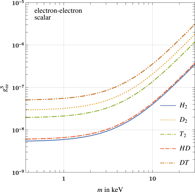
(a) Scalar electron–electron interaction.

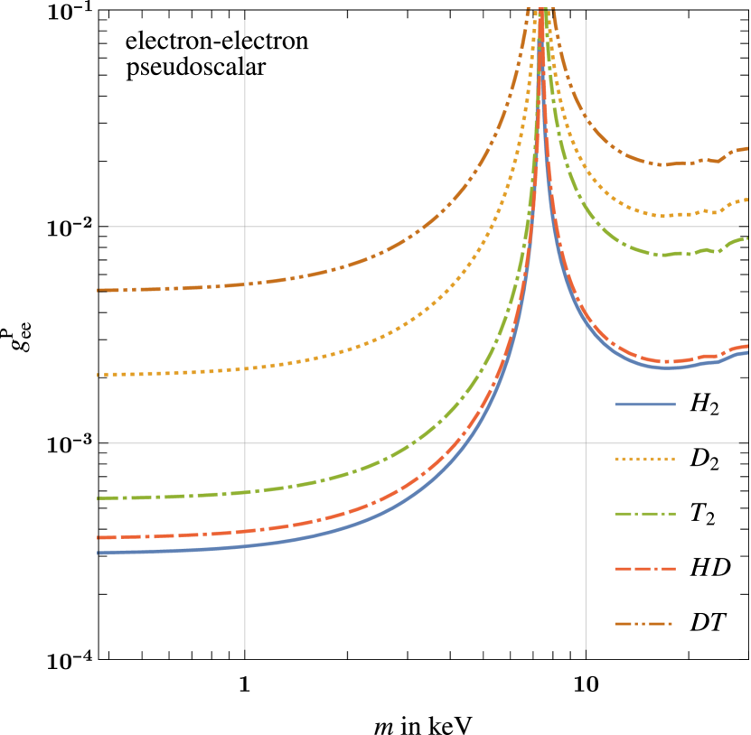
(b) Pseudoscalar electron–electron interaction.

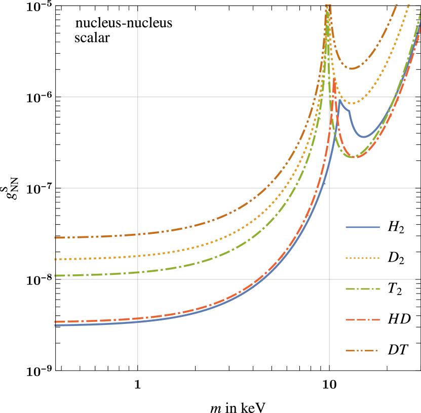
(c) Scalar nucleus–nucleus interaction.
 

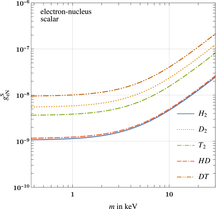
(d) Scalar electron–nucleus interaction with positive coupling $g^{\mathrm{S}}_{\mathrm{eN}}>0$.

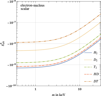
(e) Scalar electron–nucleus interaction with negative coupling $g^{\mathrm{S}}_{\mathrm{eN}}<0$.

Figure 1: Exclusion limits in mass–coupling plane on forces mediated by scalar or pseudoscalar particles. For each molecule, the corresponding upper limit results from the combination of all available measurements. The area above the curves is excluded.

 

For a pure nucleus–nucleus interaction, a pseudoscalar contribution is even more suppressed by $m^{2}/m_{\mathrm{N}}^{2}\sim 10^{-11}$, thus, we only consider the scalar potential. The corresponding limits in the mass-coupling plane are shown in Figure 1(c). Kinks in the plot are an artefact of the combination of several measured lines indicating that another measurement becomes more efficient in the exclusion of parameter space. While the dominant limits of $\order{10^{-8}}$ for masses $\lesssim$10\text{\,}\mathrm{keV}$$ arise from H₂ and HD transitions, T₂ measurements are most constraining for larger masses. Note that our limits are weaker than the ones presented in References [25, 58] as a consequence of a more conservative exclusion criterion by allowing for $3\sigma$ deviations.

In the case of an electron–nucleus interaction the spin matrix elements for the electronic ground state vanish and thus only the scalar interaction survives. Since the relative sign of the electron and nucleus coupling $g^{\mathrm{S}}_{\mathrm{eN}}$ is not fixed, we show the exclusion limits for both signs in Figures 1(d) and 1(e). As in the electron–electron case, the strongest constraints are again given by the transitions measured in H₂ and HD molecules with upper limits on the coupling $\absolutevalue{g^{\mathrm{S}}_{\mathrm{eN}}}$ up to $\order{10^{-8}}$ and $\order{10^{-9}}$ for a positive and negative coupling, respectively. Compared to the electron–electron and nucleus–nucleus case, the slightly better constraints are expected because of the four possible combinations of electrons and nuclei. Note that there should be another enhancement due to $g^{\mathrm{S}}_{\mathrm{eN}}$ also implying a $g^{\mathrm{S}}_{\mathrm{ee}}$ and $g^{\mathrm{S}}_{\mathrm{NN}}$ coupling, however, the order of magnitude will not change.

3.3 Vector and Axialvector Exchange Potentials

There are different options of introducing a new (axial)vector coupling. One possibility is via kinetic mixing with a “dark” photon, where a new “dark” $U(1)$ gauge field described by the field-strength tensor $F^{\prime}_{\mu\nu}=\partial_{\mu}A^{\prime}_{\nu}-\partial_{\nu}A^{\prime}_{\mu}$ mixes with the electromagnetic photon through a Lagrangian of the type [35]

$$\mathcal{L}_{\text{kin-mix}}=-\frac{1}{4}F^{\mu\nu}F_{\mu\nu}-\frac{1}{4}F^{\prime\mu\nu}F^{\prime}_{\mu\nu}-\frac{1}{2}F^{\mu\nu}F^{\prime}_{\mu\nu}\,.$$ (22)

Another possibility involves the Stueckelberg mechanism where additionally a light axion-like field is present [76, 77]. In this case, the heavy vector is usually referred to a $Z^{\prime}$ boson and thus supposed to have a mass in the $\mathrm{GeV}$ regime rather than $\mathrm{keV}$.

The presence of a light spin-1 mediator with vector and axialvector couplings $g^{\mathrm{V,A}}_{\mathrm{ab}}=g^{\mathrm{V,A}}_{\mathrm{a}}g^{\mathrm{V,A}}_{\mathrm{b}}$ of the type $A_{\mu}^{\prime}\;\bar{\psi}\;\gamma^{\mu}\left(g^{\mathrm{V}}_{\psi}+\mathrm{i}\,\gamma_{5}\;g^{\mathrm{A}}_{\psi}\right)\psi$ and a mass $m$ leads to non-relativistic potentials [29]

$$V_{\mathrm{V}}(\mathbf{r})=\; \frac{g^{\mathrm{V}}_{\mathrm{ab}}}{4\pi}\;\frac{\mathrm{e}^{-mr}}{r}\bigg{\{}1+$$

$$\qquad\frac{m^{2}}{4m_{\mathrm{a}}m_{\mathrm{b}}}\bigg{[}\bm{\sigma}_{\mathrm{a}}\cdot\bm{\sigma}_{\mathrm{b}}\left(\frac{1}{m^{2}r^{2}}+\frac{1}{mr}+1-\frac{8\pi r}{3m^{2}}\delta(\mathbf{r})\right)$$

$$\qquad\qquad\qquad\qquad-(\bm{\sigma}_{\mathrm{a}}\cdot\hat{\mathbf{r}})(\bm{\sigma}_{\mathrm{b}}\cdot\hat{\mathbf{r}})\left(\frac{3}{m^{2}r^{2}}+\frac{3}{mr}+1\right)\bigg{]}\bigg{\}}\,,$$ (23a)

$$V_{\mathrm{A}}(\mathbf{r})=\; -\frac{g^{\mathrm{A}}_{\mathrm{ab}}}{4\pi}\frac{\mathrm{e}^{-mr}}{r}\bigg{\{}\;\bm{\sigma}_{\mathrm{a}}\cdot\bm{\sigma}_{\mathrm{b}}\bigg{[}1+\frac{1}{m^{2}r^{2}}+\frac{1}{mr}+\frac{4\pi r}{3m^{2}}\delta^{(3)}(\mathbf{r})\bigg{]}$$

$$\qquad\qquad\qquad\qquad-(\bm{\sigma}_{\mathrm{a}}\cdot\hat{\mathbf{r}})(\bm{\sigma}_{\mathrm{b}}\cdot\hat{\mathbf{r}})\bigg{[}1+\frac{3}{m^{2}r^{2}}+\frac{3}{mr}\bigg{]}\bigg{\}}\,.$$ (23b)

Here, $\bm{\sigma}_{i}$ and $\hat{\mathbf{r}}$ are the Pauli matrices of particle $i$ and the unit vector pointing in the direction between the two fermions a and b, respectively.

The dominant spin-independent effect can be found from the $V_{\mathrm{V}}$ potential above, being exactly the Yukawa-type potential mentioned earlier. Note that the spin-dependent vector interactions are suppressed by the fermion masses. Thus, the leading contribution for a vector mediator is given by the Yukawa potential

$$V_{\text{V}}(\mathbf{r})=\pm\frac{g^{\text{V}}_{\mathrm{ab}}}{4\pi}\frac{\mathrm{e}^{-mr}}{r}\,.$$ (24)

In contrast to the pseudoscalar case, the axial vector interaction is not suppressed by the inverse fermion masses. The contribution from the axialvector potential is expected to be of the same size as the leading vector contribution, where additionally the dependence on the mediator mass plays a more significant role. As for the pseudoscalar case, the potentials have been derived for an interaction among fermions and, hence, we only consider the leading Yukawa-type contribution for bosonic nuclei.

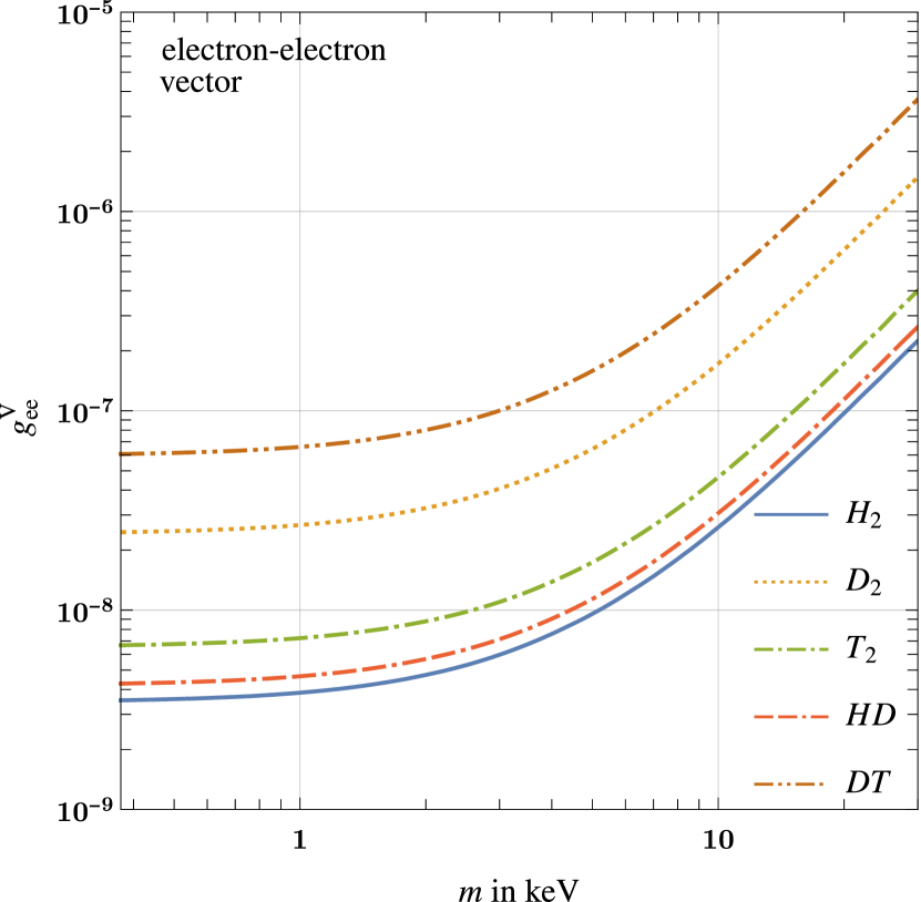
(a) Vector electron–electron interaction.

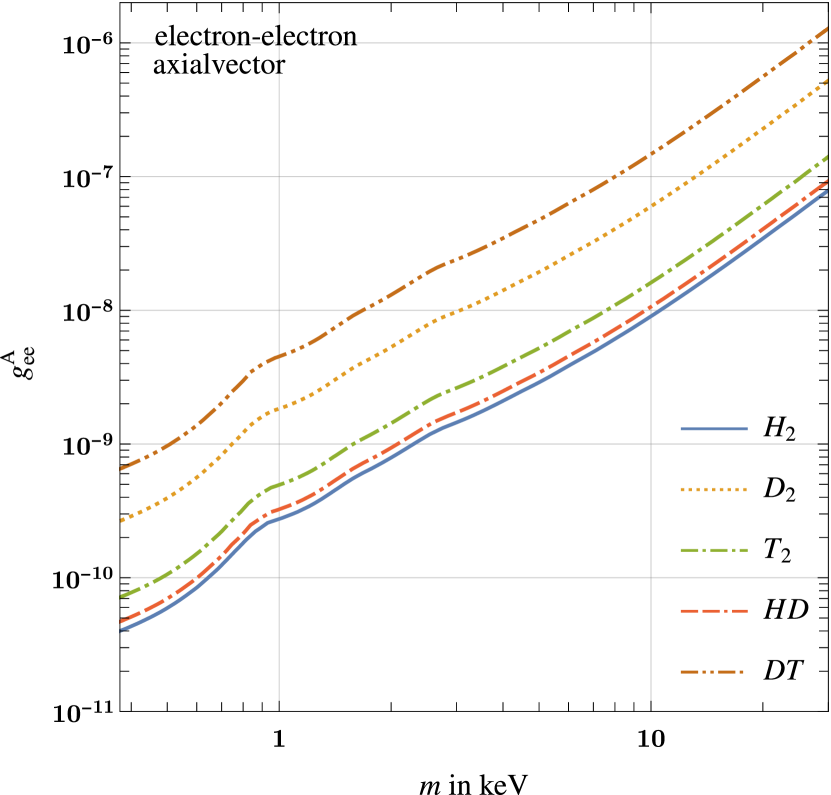
(b) Axialvector electron–electron interaction.

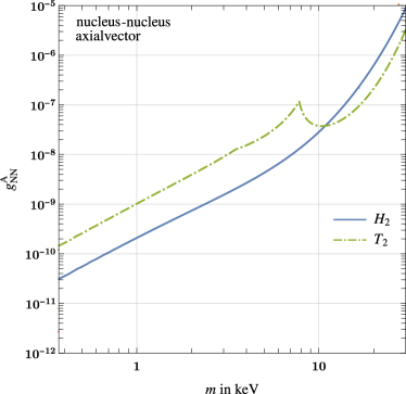
(c) Axialvector nucleus–nucleus interaction.

Figure 2: Exclusion limits in mass–coupling plane on forces mediated by vector or axialvector particles. For each molecule, the corresponding upper limit on the coupling constants results from the combination of all available measurements.

 

Like in the scalar interaction, the strongest constraints for a pure electronic force are given by the measurement of H₂ and HD transition, see Figures 2(a) and 2(b). We find an upper limit on the coupling $g^{\mathrm{V,A}}_{\mathrm{ee}}$ of $\order{10^{-8}}$ and $\order{10^{-10}}$ for the vector and axialvector potential, respectively, for masses around $1\text{\,}\mathrm{keV}$.

Regarding the nucleus–nucleus force, the additional terms in the vector contribution are suppressed by two powers of the nuclear mass and, therefore, the limits coincide with the ones for the scalar potential shown in Figure 1(c). Bounds from the axialvector exchange are again stronger by two orders of magnitude yielding an upper bound on the coupling $g_{\mathrm{NN}}^{\mathrm{A}}$ of $\order{10^{-10}}$, see Figure 2(c). Since we do not consider the bosonic nuclei D₂ and HD, the best limits are now given by H₂ measurements for masses below $10\text{\,}\mathrm{k}\mathrm{e}\mathrm{V}$ and by T₂ lines for larger masses.

Analogously to the pseudoscalar electron–nucleus interaction, the spin-dependent terms vanish for the electronic ground state of H₂ isotopologues. As a consequence, the bounds on the vector potential are the same as for the scalar case, see Figures 1(d) and 1(e), while an axialvector force vanishes entirely.

3.4 Singular Potentials: Effective Contact Interactions

The Standard Model already comprises a suppressed short-range Yukawa-like potential mediated by the heavy electroweak vector bosons or the scalar Higgs boson. According to the decoupling theorem, these interactions should not have any effect on atomic or molecular scales so that they can be safely ignored. However, there are claims in the literature that an effective coupling mediated by heavy $W$​, $Z$ or the Higgs boson leads to a measurable two-particle exchange of a very light mediator. This two-fermion exchange may induce long-range forces as pointed out in the literature [69, 78, 79, 80, 81, 5, 82, 83, 84, 85], see Figure 3. For instance, the case of an effective Fermi interaction with massless neutrinos has been first discussed by Feinberg and Sucher in the late 1960s [69] and was completed by Hsu and Sikivie in the early 1990s [79]. Their work has been extended by Grifols et al. [80] to the case of massive Dirac and Majorana-type neutrinos of mass $m_{\nu}$, yielding the long-range potentials

$$V_{\mathrm{M}}(r) =\frac{G_{\text{eff}}^{2}m_{\nu}^{2}}{8\pi^{2}r^{3}}\;K_{2}(2m_{\nu}r)\stackrel{{\scriptstyle m_{\nu}r\gg 1}}{{\approx}}\frac{G_{\text{eff}}}{16\pi^{2}r^{2}}\sqrt{\frac{m_{\nu}^{3}}{\pi r^{3}}}\operatorname{e}^{-2m_{\nu}r}\,,$$ (25a)

$$V_{\mathrm{D}}(r) =\frac{G_{\mathrm{eff}}^{2}m_{\nu}^{3}}{16\pi^{3}r^{2}}\;K_{3}(2m_{\nu}r)\stackrel{{\scriptstyle m_{\nu}r\gg 1}}{{\approx}}\frac{G_{\text{eff}}}{32\pi^{2}}\sqrt{\frac{m_{\nu}^{5}}{\pi r^{5}}}\operatorname{e}^{-2m_{\nu}r}\,,$$ (25b)

with the modified Bessel functions $K_{n}$. In the Standard Model case, the effective coupling $G_{\text{eff}}$ is given by the Fermi constant $G_{\mathrm{F}}$. Both potentials scale like $\sim 1/r^{5}$ in the limit of vanishing neutrino masses or short distances, reproducing the well-known result by Feinberg and Sucher [69],

$$V(r)=\frac{G_{\mathrm{eff}}^{2}}{16\pi^{3}r^{5}}\,.$$ (26)

Due to the highly singular behaviour of the two-neutrino exchange potential, one needs to be careful in the analysis. Naively, we expect a quadratic divergence in our integrals from power-counting, matching Stadnik’s observation for hydrogen atoms in Reference [82]. Assuming a cut-off of the $Z$ boson mass $M_{\mathrm{Z}}$ for the integrals to account for the limited validity of the effective theory, Stadnik derives tight bounds on the coupling $G_{\text{eff}}$ close to the Standard Model value for positronium. However, we doubt the adequateness of such a cut-off, as remarked by other authors [86, 87]. The strong dependence of a result on the arbitrary value of the cut-off parameter signals an incorrect treatment of the ultraviolet divergences of the theory, bearing in mind that already at the inverse Compton wavelength of the electron much below $M_{\text{Z}}$ the physics of the pure two-neutrino potential changes.

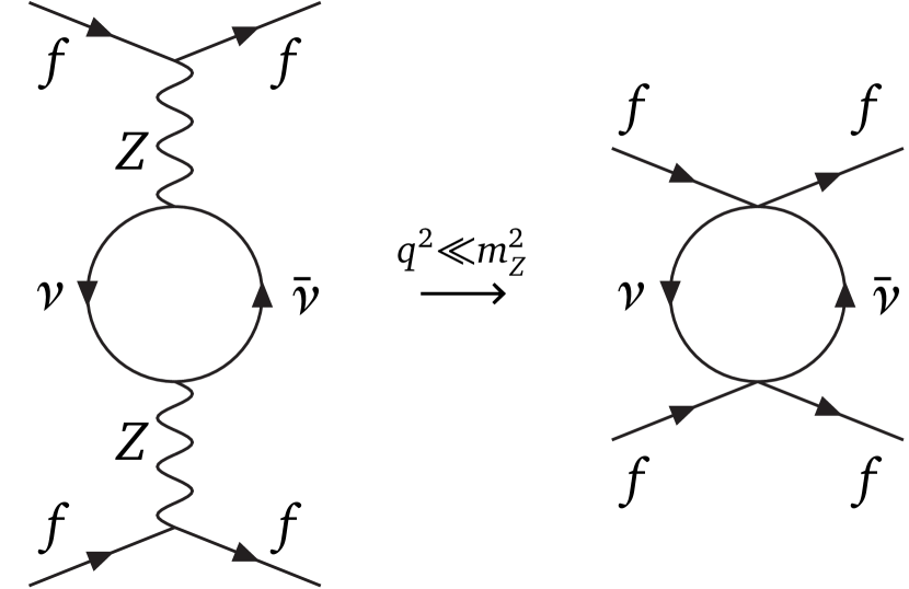
Figure 3: Long-range force mediated by double neutrino exchange (left) and double (Pseudo-)Goldstone boson exchange. In both cases, the direct coupling to the fermions is by a heavy particle ($Z$ or Higgs boson) leading to effective four-particle interactions.

 

A correct treatment involving a proper matching in the tower of effective theories at each scale in the problem is subtle and beyond the scope of this analysis. In order to get an impression of the magnitude of the neutrino exchange effects, we calculate the short-range effect to the molecular levels caused by the exchange of a $W$ boson with mass $M_{\mathrm{W}}$ as depicted in the diagram in Figure 4. Parametrically, the effects of both this $W$ box diagram and the neutrino exchange are of order $\order{G_{\mathrm{F}}^{2}M_{\mathrm{W}}^{2}}$. We are rather expecting a further suppression, for instance due to small mixing factors in the case of sterile neutrinos. Evaluating the box diagram, we derive the effective low-energy potential

$$V_{W\mathrm{box}}(\mathbf{r})=\frac{4}{3}\pi G_{\mathrm{F}}^{2}M_{\mathrm{W}}^{2}\delta^{(3)}(\mathbf{r})\,.$$ (27)

The size of this effect is of $\order{${10}^{-11}\text{\,}\mathrm{c}\mathrm{m}^{-1}$}$ and, hence, far below the current experimental sensitivity. Due to its smallness, the neutrino exchange is negligible if the Coulomb force is present and one may rather expect an effect in cases where the electromagnetic force is absent or screened like between neutral atoms and molecules, as has been noted in Reference [69].

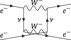
Figure 4: Additional contribution to the two-neutrino force induced by a $W$-box diagram.

 

The two-neutrino exchange has recently been studied in the context of atomic parity violation [88, 84]. By using higher angular momentum transitions, the authors are able to derive limits from wave functions dropping rapidly for small distances, which seems to be a suitable approach to deal with the divergence. However, their analysis is missing a full systematic treatment of all matchings at intermediate scales, which might have an influence on the results. Nevertheless, the effect is far below the reach of current and future experiments, similar to our estimate. The study of Reference [88] goes beyond the known physics properties of electroweak physics and constrains new models extending the Standard Model, especially with an extra Higgs doublet or a light $Z^{\prime}$. A recent discussion of the full effective theory framework of the long-range neutrino potential has been given in [85].

There are further modifications of the intramolecular forces possible due to Higgs and Goldstone boson exchange, where a long-range potential arises in a similar manner as for neutrinos [81], see Figure 3. In particular, a massive (pseudo)scalar boson $a$ of mass $m$ interacting with the Standard Model Higgs boson $H$ via the Lagrangian $\mathcal{L}_{\mathrm{Haa}}=g_{\mathrm{Haa}}\>aaH$ yields the potential

$$V_{\text{PG}}(r)=-\frac{G\,m}{8\pi^{3}r^{2}}K_{1}(2mr)\,.$$ (28)

Here, the coupling strength $G$ is related to the Standard Model Higgs-fermion interaction $g_{\mathrm{Hff}}$ by [81]

$$G=\frac{g_{\mathrm{Hff}}g_{\mathrm{Hf^{\prime}f^{\prime}}}g_{\mathrm{Haa}}^{2}}{m_{\mathrm{H}}^{4}}\sim${10}^{-19}\text{\,}\mathrm{G}\mathrm{eV}^{-4}$g_{\mathrm{Haa}}^{2}\,.$$ (29)

Although the potential reduces to a well-behaved $1/r^{3}$ functional form for small masses $m$, the tiny prefactor renders this process impossible to observe in molecular spectra.

4 Conclusions

In the present work, we have performed the first extensive and systematic study of New Physics effects on molecular spectra. Starting from available codes which give precise ab initio predictions in the Standard Model for transitions in hydrogen-like molecules, we treated a variety of New Physics potentials as perturbations and derived constraints on the new forces from direct measurements.

Molecular spectroscopy, as well as atomic spectroscopy, essentially probes the Coulomb potential and Quantum Electrodynamics with high accuracy. From our analysis we conclude that New Physics effects are unlikely to be seen in spectroscopy at all. Spectroscopical observations of sufficiently large deviations would be in conflict with indirect constraints stemming from astrophysics and cosmology. Nevertheless, spectroscopy is a complementary and direct test of the Standard Model in the laboratory and is an important tool in the context of New Physics searches in this only indirectly excluded parameter region. Despite the expectation that heavier nuclei as in tritiated molecules give stronger constraints than hydrogen alone, we do not observe higher sensitivity in the isotopologues compared to hydrogen.

We have found that constraints on new interactions between electrons and nuclei from molecular spectroscopy are compatible with atomic spectroscopy, but the latter derives more stringent bounds of up to three orders of magnitude. The same is true for probes of the nucleus–nucleus interaction from rovibrational spectroscopy compared to direct neutron scattering. Furthermore, in the case of a modified electron–electron coupling, molecular spectroscopy is competitive with Helium spectroscopy, although there are stronger limits of approximately two orders of magnitude on the coupling $g_{\mathrm{NP}}$ available from measurements of the anomalous magnetic moment of the electron.

As an advantage to other direct techniques molecular spectroscopy allows to probe a plethora of New Physics interactions between different types of particles in one single measurement—assuming that only one type of interaction is present at the time. Further improvements in both theoretical treatment of hydrogen-like molecules and experimental precision are going to yield stronger constraints. Moreover, we have found relatively loose constraints for a certain mass window of the mediator particle for some potentials. In case of spin-dependent forces, polarized probes may help to improve the exclusion limits.

Searches for a new long-range force mediated by an exchange of two light particles like neutrinos are not promising in spectroscopy since the expected effect is too small due to parametric suppression. Furthermore, a strong cut-off dependence appears when divergences in the theory are not properly taken into account so that the sensitivity is misestimated. A full treatment of the effective theories at all scales down to very short distances is beyond the scope of this paper. In any case, we do not expect an effect that is going to be visible in the next generation experiments.

During the finalization of this work, we got aware of a new set of measurements including more lines for T₂, DT, and HT [89]. This study shows very good agreement with the theoretical prediction.

Appendix A Experimental data

Here, we list all experimental data that were used in our analysis in Section 3.

Table 2: List of all measurements used in our analysis. The transitions $(v_{1},J_{1})\rightarrow(v_{2},J_{2})$ are characterized by the vibrational quantum numbers $v_{i}$ and the angular momentums $J_{i}$ of the involved levels $(v_{i},J_{i})$. All numbers are given in $\mathrm{c}\mathrm{m}^{-1}$.

molecule	transition	energy	reference
H2	$(3,5)$ $\rightarrow$ $(0,3)$	$12\,559.749\,52(5)$	[90]
H2	$(1,0)$ $\rightarrow$ $(0,0)$	$4161.166\,36(15)$	[54]
H2	$(1,1)$ $\rightarrow$ $(0,1)$	$4155.254\,00(21)$	[54]
H2	$(1,2)$ $\rightarrow$ $(0,2)$	$4143.465\,53(15)$	[54]
H2	$(11,1)$ $\rightarrow$ $(0,0)$	$32\,937.7554(16)$	[91]
H2	$(11,3)$ $\rightarrow$ $(0,0)$	$33\,186.4791(16)$	[91]
H2	$(11,4)$ $\rightarrow$ $(0,0)$	$33\,380.1025(33)$	[91]
H2	$(11,5)$ $\rightarrow$ $(0,0)$	$33\,615.5371(18)$	[91]
HD	$(1,0)$ $\rightarrow$ $(0,0)$	$3632.160\,52(22)$	[54]
HD	$(1,1)$ $\rightarrow$ $(0,1)$	$3628.304\,50(22)$	[54]
HD	$(2,2)$ $\rightarrow$ $(0,1)$	$7241.849\,350\,87(67)$	[55]
HD	$(2,3)$ $\rightarrow$ $(0,2)$	$7306.483\,222\,50(93)$	[55]
HD	$(2,4)$ $\rightarrow$ $(0,3)$	$7361.903\,173\,35(93)$	[55]
D2	$(1,0)$ $\rightarrow$ $(0,0)$	$2993.617\,06(15)$	[54]
D2	$(1,1)$ $\rightarrow$ $(0,1)$	$2991.507\,06(15)$	[54]
D2	$(1,2)$ $\rightarrow$ $(0,2)$	$2987.293\,52(15)$	[54]
D2	$(0,2)$ $\rightarrow$ $(0,0)$	$179.068(2)$	[68]
D2	$(0,3)$ $\rightarrow$ $(0,1)$	$297.533(3)$	[68]
D2	$(0,4)$ $\rightarrow$ $(0,2)$	$414.648(2)$	[68]
T2	$(1,0)$ $\rightarrow$ $(0,0)$	$2464.5052(4)$	[57]
T2	$(1,1)$ $\rightarrow$ $(0,1)$	$2463.3494(3)$	[57]
T2	$(1,2)$ $\rightarrow$ $(0,2)$	$2461.0388(4)$	[57]
T2	$(1,3)$ $\rightarrow$ $(0,3)$	$2457.5803(4)$	[57]
T2	$(1,4)$ $\rightarrow$ $(0,4)$	$2452.9817(4)$	[57]
T2	$(1,5)$ $\rightarrow$ $(0,5)$	$2447.2510(4)$	[57]
DT	$(1,0)$ $\rightarrow$ $(0,0)$	$2743.341\,71(40)$	[58]
DT	$(1,1)$ $\rightarrow$ $(0,1)$	$2741.732\,04(330)$	[58]
DT	$(1,2)$ $\rightarrow$ $(0,2)$	$2738.516\,59(40)$	[58]
DT	$(1,3)$ $\rightarrow$ $(0,3)$	$2733.704\,70(40)$	[58]
DT	$(1,4)$ $\rightarrow$ $(0,4)$	$2727.307\,34(40)$	[58]
DT	$(1,5)$ $\rightarrow$ $(0,5)$	$2719.341\,93(40)$	[58]

References

- [1] S. Knapen, T. Lin, and K. M. Zurek, “Light Dark Matter: Models and Constraints”, Phys. Rev. D96 no. 11, (2017) 115021, arXiv:1709.07882 [hep-ph].
- [2] J. A. Dror, G. Elor, and R. Mcgehee, “Directly Detecting Signals from Absorption of Fermionic Dark Matter”, Phys. Rev. Lett. 124 no. 18, (2020) 18, arXiv:1905.12635 [hep-ph].
- [3] J. A. Dror, G. Elor, and R. Mcgehee, “Absorption of Fermionic Dark Matter by Nuclear Targets”, JHEP 02 (2020) 134, arXiv:1908.10861 [hep-ph].
- [4] A. Arvanitaki, S. Dimopoulos, and K. Van Tilburg, “Resonant absorption of bosonic dark matter in molecules”, Phys. Rev. X8 no. 4, (2018) 041001, arXiv:1709.05354 [hep-ph].
- [5] S. Fichet, “Quantum Forces from Dark Matter and Where to Find Them”, Phys. Rev. Lett. 120 no. 13, (2018) 131801, arXiv:1705.10331 [hep-ph].
- [6] P. Brax, S. Fichet, and G. Pignol, “Bounding Quantum Dark Forces”, Phys. Rev. D97 no. 11, (2018) 115034, arXiv:1710.00850 [hep-ph].
- [7] W. Kolos and L. Wolniewicz, “A complete non-relativistic treatment of the H2 molecule”, Physics Letters 2 no. 5, (1962) 222–223. https://doi.org/10.1016/0031-9163(62)90235-4.
- [8] W. Kołos and L. Wolniewicz, “Nonadiabatic theory for diatomic molecules and its application to the hydrogen molecule”, Reviews of Modern Physics 35 no. 3, (1963) 473–483. https://doi.org/10.1103/RevModPhys.35.473.
- [9] W. Kołos and L. Wolniewicz, “Accurate Adiabatic Treatment of the Ground State of the Hydrogen Molecule”, The Journal of chemical physics 41 no. 12, (1964) 3663–3673. https://doi.org/10.1063/1.1725796.
- [10] W. Kołos and L. Wolniewicz, “Accurate computation of vibronic energies and of some expectation values for H2, D2, and T2”, The Journal of chemical physics 41 no. 12, (1964) 3674–3678. https://doi.org/10.1063/1.1725797.
- [11] W. Kołos and L. Wolniewicz, “Improved theoretical ground-state energy of the hydrogen molecule”, The Journal of chemical physics 49 no. 1, (1968) 404–410. https://doi.org/10.1063/1.1669836.
- [12] K. Pachucki and J. Komasa, “Nonadiabatic corrections to the wave function and energy”, Journal of Chemical Physics 129 no. 3, (2008) . https://www.scopus.com/inward/record.uri?eid=2-s2.0-47849090977&doi=10.1063%2f1.2952517&partnerID=40&md5=e010a4eb52b57211614b28f17a58e5b3. cited By 47.
- [13] K. Pachucki and J. Komasa, “Nonadiabatic corrections to rovibrational levels of H2”, The Journal of Chemical Physics 130 no. 16, (2009) 164113, https://doi.org/10.1063/1.3114680. https://doi.org/10.1063/1.3114680.
- [14] K. Pachucki and J. Komasa, “Rovibrational levels of HD”, Phys. Chem. Chem. Phys. 12 (2010) 9188–9196. http://dx.doi.org/10.1039/C0CP00209G.
- [15] K. Pachucki and J. Komasa, “Leading order nonadiabatic corrections to rovibrational levels of H2, D2, and T2”, The Journal of Chemical Physics 143 no. 3, (2015) 034111, https://doi.org/10.1063/1.4927079. https://doi.org/10.1063/1.4927079.
- [16] M. Puchalski, J. Komasa, P. Czachorowski, and K. Pachucki, “Nonadiabatic QED correction to the dissociation energy of the hydrogen molecule”, Phys. Rev. Lett. 122 no. 10, (2019) 103003, arXiv:1812.02980 [physics.atom-ph].
- [17] M. Puchalski, J. Komasa, P. Czachorowski, and K. Pachucki, “Nonadiabatic QED Correction to the Dissociation Energy of the Hydrogen Molecule”, Phys. Rev. Lett. 122 (Mar, 2019) 103003. https://link.aps.org/doi/10.1103/PhysRevLett.122.103003.
- [18] M. Puchalski, J. Komasa, A. Spyszkiewicz, and K. Pachucki, “Dissociation energy of molecular hydrogen isotopologues”, Phys. Rev. A 100 (Aug, 2019) 020503. https://link.aps.org/doi/10.1103/PhysRevA.100.020503.
- [19] M. Puchalski, J. Komasa, P. Czachorowski, and K. Pachucki, “Complete Corrections to the Ground State of ”, Phys. Rev. Lett. 117 (Dec, 2016) 263002. https://link.aps.org/doi/10.1103/PhysRevLett.117.263002.
- [20] M. Puchalski, J. Komasa, and K. Pachucki, “Relativistic corrections for the ground electronic state of molecular hydrogen”, Phys. Rev. A 95 (May, 2017) 052506. https://link.aps.org/doi/10.1103/PhysRevA.95.052506.
- [21] M. Puchalski, A. Spyszkiewicz, J. Komasa, and K. Pachucki, “Nonadiabatic Relativistic Correction to the Dissociation Energy of , , and HD”, Phys. Rev. Lett. 121 (Aug, 2018) 073001. https://link.aps.org/doi/10.1103/PhysRevLett.121.073001.
- [22] P. Czachorowski, J. Komasa, G. Łach, K. Pachucki, and M. Puchalski, “H2SPECTRE”. https://www.fuw.edu.pl/~krp/codes.html; https://qcg.home.amu.edu.pl/qcg/puclic_html/H2Spectre.html.
- [23] P. Czachorowski, Relativistic nonadiabatic corrections to the ground state of molecular hydrogen. PhD thesis, University of Warsaw, 2019.
- [24] J. Komasa, M. Puchalski, P. Czachorowski, G. Łach, and K. Pachucki, “Rovibrational energy levels of the hydrogen molecule through nonadiabatic perturbation theory”, Phys. Rev. A 100 (Sep, 2019) 032519. https://link.aps.org/doi/10.1103/PhysRevA.100.032519.
- [25] E. J. Salumbides, J. C. J. Koelemeij, J. Komasa, K. Pachucki, K. S. E. Eikema, and W. Ubachs, “Bounds on fifth forces from precision measurements on molecules”, Phys. Rev. D87 no. 11, (2013) 112008, arXiv:1304.6560 [physics.atom-ph].
- [26] E. J. Salumbides, W. Ubachs, and V. I. Korobov, “Bounds on fifth forces at the sub-Angstrom length scale”, J. Molec. Spectrosc. 300 (2014) 65, arXiv:1308.1711 [hep-ph].
- [27] E. J. Salumbides, A. N. Schellekens, B. Gato-Rivera, and W. Ubachs, “Constraints on extra dimensions from precision molecular spectroscopy”, New J. Phys. 17 no. 3, (2015) 033015, arXiv:1502.02838 [physics.atom-ph].
- [28] J. Jaeckel and S. Roy, “Spectroscopy as a test of Coulomb’s law: A Probe of the hidden sector”, Phys. Rev. D82 (2010) 125020, arXiv:1008.3536 [hep-ph].
- [29] P. Fadeev, Y. V. Stadnik, F. Ficek, M. G. Kozlov, V. V. Flambaum, and D. Budker, “Revisiting spin-dependent forces mediated by new bosons: Potentials in the coordinate-space representation for macroscopic- and atomic-scale experiments”, Phys. Rev. A99 no. 2, (2019) 022113, arXiv:1810.10364 [hep-ph].
- [30] A. Costantino, S. Fichet, and P. Tanedo, “Exotic Spin-Dependent Forces from a Hidden Sector”, JHEP 03 (2020) 148, arXiv:1910.02972 [hep-ph].
- [31] V. Silveira and A. Zee, “SCALAR PHANTOMS”, Phys. Lett. 161B (1985) 136–140.
- [32] J. McDonald, “Gauge singlet scalars as cold dark matter”, Phys. Rev. D50 (1994) 3637–3649, arXiv:hep-ph/0702143 [HEP-PH].
- [33] J. E. Moody and F. Wilczek, “New macroscopic forces?”, Phys. Rev. D30 (1984) 130.
- [34] J. Jaeckel and A. Ringwald, “The Low-Energy Frontier of Particle Physics”, Ann. Rev. Nucl. Part. Sci. 60 (2010) 405–437, arXiv:1002.0329 [hep-ph].
- [35] B. Holdom, “Two U(1)’s and Epsilon Charge Shifts”, Phys. Lett. 166B (1986) 196–198.
- [36] P. Fayet, “Extra U(1)’s and New Forces”, Nucl. Phys. B347 (1990) 743–768.
- [37] R. Essig et al., “Working Group Report: New Light Weakly Coupled Particles”, in Proceedings, 2013 Community Summer Study on the Future of U.S. Particle Physics: Snowmass on the Mississippi (CSS2013): Minneapolis, MN, USA, July 29-August 6, 2013. 2013. arXiv:1311.0029 [hep-ph].
- [38] C. Delaunay, C. Frugiuele, E. Fuchs, and Y. Soreq, “Probing new spin-independent interactions through precision spectroscopy in atoms with few electrons”, Phys. Rev. D96 no. 11, (2017) 115002, arXiv:1709.02817 [hep-ph].
- [39] J. C. Berengut et al., “Probing New Long-Range Interactions by Isotope Shift Spectroscopy”, Phys. Rev. Lett. 120 (2018) 091801, arXiv:1704.05068 [hep-ph].
- [40] M. P. A. Jones, R. M. Potvliege, and M. Spannowsky, “Probing new physics using Rydberg states of atomic hydrogen”, arXiv:1909.09194 [hep-ph].
- [41] Y. Kamiya, K. Itagaki, M. Tani, G. N. Kim, and S. Komamiya, “Constraints on New Gravitylike Forces in the Nanometer Range”, Phys. Rev. Lett. 114 (2015) 161101, arXiv:1504.02181 [hep-ex].
- [42] P. Brax and C. Burrage, “Atomic Precision Tests and Light Scalar Couplings”, Phys. Rev. D83 (2011) 035020, arXiv:1010.5108 [hep-ph].
- [43] S. Villalba-Chavez, A. Golub, and C. Muller, “Axion-modified photon propagator, Coulomb potential and Lamb-shift”, Phys. Rev. D98 no. 11, (2018) 115008, arXiv:1806.10940 [hep-ph].
- [44] G. G. Raffelt, “Astrophysical methods to constrain axions and other novel particle phenomena”, Phys. Rept. 198 (1990) 1–113.
- [45] G. G. Raffelt, Stars as laboratories for fundamental physics. Chicago, USA: Univ. Pr. (1996) 664 p, 1996. http://wwwth.mpp.mpg.de/members/raffelt/mypapers/199613.pdf.
- [46] G. G. Raffelt, “Astrophysical axion bounds”, Lect. Notes Phys. 741 (2008) 51–71, arXiv:hep-ph/0611350 [hep-ph].
- [47] P. F. Depta, M. Hufnagel, and K. Schmidt-Hoberg, “Robust cosmological constraints on axion-like particles”, arXiv:2002.08370 [hep-ph].
- [48] G. Carugno, Z. Fontana, R. Onofrio, and C. Rizzo, “Limits on the existence of scalar interactions in the submillimeter range”, Phys. Rev. D55 (1997) 6591–6595.
- [49] T. A. Wagner, S. Schlamminger, J. H. Gundlach, and E. G. Adelberger, “Torsion-balance tests of the weak equivalence principle”, Class. Quant. Grav. 29 (2012) 184002, arXiv:1207.2442 [gr-qc].
- [50] G. L. Klimchitskaya and V. M. Mostepanenko, “Constraints on axion and corrections to Newtonian gravity from the Casimir effect”, Grav. Cosmol. 21 no. 1, (2015) 1–12, arXiv:1502.07647 [hep-ph].
- [51] G. L. Klimchitskaya and V. M. Mostepanenko, “Constraints on axionlike particles and non-Newtonian gravity from measuring the difference of Casimir forces”, Phys. Rev. D95 no. 12, (2017) 123013, arXiv:1704.05892 [hep-ph].
- [52] A. Dupays, E. Masso, J. Redondo, and C. Rizzo, “Light scalars coupled to photons and non-newtonian forces”, Phys. Rev. Lett. 98 (2007) 131802, arXiv:hep-ph/0610286 [hep-ph].
- [53] G. D. Dickenson, M. L. Niu, E. J. Salumbides, J. Komasa, K. S. E. Eikema, K. Pachucki, and W. Ubachs, “Fundamental Vibration of Molecular Hydrogen”, Phys. Rev. Lett. 110 (May, 2013) 193601. https://link.aps.org/doi/10.1103/PhysRevLett.110.193601.
- [54] M. Niu, E. Salumbides, G. Dickenson, K. Eikema, and W. Ubachs, “Precision spectroscopy of the rovibrational splittings in H2, HD and D2”, Journal of Molecular Spectroscopy 300 (2014) 44 – 54. http://www.sciencedirect.com/science/article/pii/S0022285214000630. Spectroscopic Tests of Fundamental Physics.
- [55] F. M. J. Cozijn, P. Dupré, E. J. Salumbides, K. S. E. Eikema, and W. Ubachs, “Sub-Doppler Frequency Metrology in HD for Tests of Fundamental Physics”, Phys. Rev. Lett. 120 (Apr, 2018) 153002. https://link.aps.org/doi/10.1103/PhysRevLett.120.153002.
- [56] M. Schlösser, X. Zhao, M. Trivikram, W. Ubachs, and E. J. Salumbides, “CARS spectroscopy of the band in ”, Journal of Physics B: Atomic, Molecular and Optical Physics 50 no. 21, (Oct, 2017) 214004. https://doi.org/10.1088%2F1361-6455%2Faa8d80.
- [57] T. M. Trivikram, M. Schlösser, W. Ubachs, and E. J. Salumbides, “Relativistic and QED Effects in the Fundamental Vibration of ”, Phys. Rev. Lett. 120 (Apr, 2018) 163002. https://link.aps.org/doi/10.1103/PhysRevLett.120.163002.
- [58] K.-F. Lai, P. Czachorowski, M. Schlösser, M. Puchalski, J. Komasa, K. Pachucki, W. Ubachs, and E. J. Salumbides, “Precision tests of nonadiabatic perturbation theory with measurements on the DT molecule”, Phys. Rev. Research 1 (Nov, 2019) 033124. https://link.aps.org/doi/10.1103/PhysRevResearch.1.033124.
- [59] W. Heitler and F. London, “Wechselwirkung neutraler Atome und homöopolare Bindung nach der Quantenmechanik”, Zeitschrift für Physik 44 no. 6, (Jun, 1927) 455–472. https://doi.org/10.1007/BF01397394.
- [60] M. Born and R. Oppenheimer, “Zur Quantentheorie der Molekeln”, Annalen der Physik 389 no. 20, 457–484. https://onlinelibrary.wiley.com/doi/abs/10.1002/andp.19273892002.
- [61] M. Born, Kopplung der Elektronen- und Kernbewegung in Molekeln und Kristallen. Nachrichten der Akademie der Wissenschaften in Göttingen, Mathematisch-Physikalische Klasse: 2a, Mathematisch-Physikalisch-Chemische Abteilung; 1951, 6. Vandenhoeck & Ruprecht, Göttingen, 1951.
- [62] H. M. James and A. S. Coolidge, “The Ground State of the Hydrogen Molecule”, The Journal of Chemical Physics 1 no. 12, (1933) 825–835, https://doi.org/10.1063/1.1749252. https://doi.org/10.1063/1.1749252.
- [63] K. Pachucki, “Born-Oppenheimer potential for ”, Phys. Rev. A 82 (Sep, 2010) 032509. https://link.aps.org/doi/10.1103/PhysRevA.82.032509.
- [64] P. Czachorowski, M. Puchalski, J. Komasa, and K. Pachucki, “Nonadiabatic relativistic correction in H2 , D2 , and HD”, Phys. Rev. A98 no. 5, (2018) 052506, arXiv:1810.02604 [physics.atom-ph].
- [65] M. Puchalski, J. Komasa, P. Czachorowski, and K. Pachucki, “Complete corrections to the ground state of H2”, Phys. Rev. Lett. 117 no. 26, (2016) 263002, arXiv:1608.07081 [physics.chem-ph].
- [66] K. Pachucki, M. Zientkiewicz, and V. Yerokhin, “H2SOLV: Fortran solver for diatomic molecules in explicitly correlated exponential basis”, Computer Physics Communications 208 (07, 2016) .
- [67] F. Biraben, “The first decades of Doppler-free two-photon spectroscopy”, Comptes Rendus Physique 20 no. 7, (2019) 671 – 681. http://www.sciencedirect.com/science/article/pii/S1631070519300283. La science en mouvement 2 : de 1940 aux premières années 1980 â Avancées en physique.
- [68] R. Z. Martínez, D. Bermejo, P. Wcisło, and F. Thibault, “Accurate wavenumber measurements for the S0(0), S0(1), and S0(2) pure rotational Raman lines of D2”, Journal of Raman Spectroscopy 50 no. 1, 127–129. https://onlinelibrary.wiley.com/doi/abs/10.1002/jrs.5499.
- [69] G. Feinberg and J. Sucher, “Long-Range Forces from Neutrino-Pair Exchange”, Phys. Rev. 166 (1968) 1638–1644.
- [70] R. D. Peccei and H. R. Quinn, “CP Conservation in the Presence of Instantons”, Phys. Rev. Lett. 38 (1977) 1440–1443.
- [71] R. D. Peccei and H. R. Quinn, “Constraints Imposed by CP Conservation in the Presence of Instantons”, Phys. Rev. D16 (1977) 1791–1797.
- [72] F. Wilczek, “Problem of Strong and Invariance in the Presence of Instantons”, Phys. Rev. Lett. 40 (1978) 279–282.
- [73] S. Weinberg, “A New Light Boson?”, Phys. Rev. Lett. 40 (1978) 223–226.
- [74] J. Preskill, M. B. Wise, and F. Wilczek, “Cosmology of the Invisible Axion”, Phys. Lett. B120 (1983) 127–132.
- [75] Y. Chikashige, R. N. Mohapatra, and R. D. Peccei, “Are There Real Goldstone Bosons Associated with Broken Lepton Number?”, Phys. Lett. 98B (1981) 265–268.
- [76] E. C. G. Stueckelberg, “Interaction energy in electrodynamics and in the field theory of nuclear forces”, Helv. Phys. Acta 11 (1938) 225–244.
- [77] B. Kors and P. Nath, “A Stueckelberg extension of the standard model”, Phys. Lett. B586 (2004) 366–372, arXiv:hep-ph/0402047 [hep-ph].
- [78] S.-J. Chang and R. Rajaraman, “Long-range corrections to the coulomb potential and their implications about weak interactions”, Phys. Rev. 183 (1969) 1442–1445.
- [79] S. D. H. Hsu and P. Sikivie, “Long range forces from two neutrino exchange revisited”, Phys. Rev. D49 (1994) 4951–4953, arXiv:hep-ph/9211301 [hep-ph].
- [80] J. A. Grifols, E. Masso, and R. Toldra, “Majorana neutrinos and long range forces”, Phys. Lett. B389 (1996) 563–565, arXiv:hep-ph/9606377 [hep-ph].
- [81] F. Ferrer and M. Nowakowski, “Higgs and Goldstone bosons mediated long range forces”, Phys. Rev. D59 (1999) 075009, arXiv:hep-ph/9810550 [hep-ph].
- [82] Y. V. Stadnik, “Probing Long-Range Neutrino-Mediated Forces with Atomic and Nuclear Spectroscopy”, Phys. Rev. Lett. 120 no. 22, (2018) 223202, arXiv:1711.03700 [physics.atom-ph].
- [83] Q. Le Thien and D. E. Krause, “Spin-Independent Two-Neutrino Exchange Potential with Mixing and -Violation”, Phys.Rev.D 99 no. 11, (2019) 116006, arXiv:1901.05345 [hep-ph].
- [84] M. Ghosh, Y. Grossman, and W. Tangarife, “Probing the two-neutrino exchange force using atomic parity violation”, arXiv:1912.09444 [hep-ph].
- [85] P. D. Bolton, F. F. Deppisch, and C. Hati, “Probing New Physics with Long-Range Neutrino Interactions: An Effective Field Theory Approach”, arXiv:2004.08328 [hep-ph].
- [86] T. Asaka, M. Tanaka, K. Tsumura, and M. Yoshimura, “Precision electroweak shift of muonium hyperfine splitting”, arXiv:1810.05429 [hep-ph].
- [87] A. Costantino and S. Fichet, “The Neutrino Casimir Force”, arXiv:2003.11032 [hep-ph].
- [88] G. Arcadi, M. Lindner, J. Martins, and F. S. Queiroz, “New Physics Probes: Atomic Parity Violation, Polarized Electron Scattering and Neutrino-Nucleus Coherent Scattering”, arXiv:1906.04755 [hep-ph].
- [89] K.-F. Lai, V. Hermann, T. Trivikram, M. Diouf, M. Schlösser, W. Ubachs, and E. Salumbides, “Precision measurement of the fundamental vibrational frequencies of tritium-bearing hydrogen molecules: T2, DT, HT”, arXiv:2003.11060 [physics.chem-ph].
- [90] C.-F. Cheng, Y. R. Sun, H. Pan, J. Wang, A.-W. Liu, A. Campargue, and S.-M. Hu, “Electric-quadrupole transition of H2 determined to precision”, Phys. Rev. A 85 (Feb, 2012) 024501. https://link.aps.org/doi/10.1103/PhysRevA.85.024501.
- [91] T. M. Trivikram, M. L. Niu, P. Wcislo, W. Ubachs, and E. J. Salumbides, “Precision measurements and test of molecular theory in highly excited vibrational states of H2 ()”, Applied Physics B 122 no. 12, (2016) 294. https://doi.org/10.1007/s00340-016-6570-1.