Supervised Domain Adaptation:
A Graph Embedding Perspective and a
Rectified Experimental Protocol
Abstract
Domain Adaptation is the process of alleviating distribution gaps between data from different domains. In this paper, we show that Domain Adaptation methods using pair-wise relationships between source and target domain data can be formulated as a Graph Embedding in which the domain labels are incorporated into the structure of the intrinsic and penalty graphs. Specifically, we analyse the loss functions of three existing state-of-the-art Supervised Domain Adaptation methods and demonstrate that they perform Graph Embedding. Moreover, we highlight some generalisation and reproducibility issues related to the experimental setup commonly used to demonstrate the few-shot learning capabilities of these methods. To assess and compare Supervised Domain Adaptation methods accurately, we propose a rectified evaluation protocol, and report updated benchmarks on the standard datasets Office31 (Amazon, DSLR, and Webcam), Digits (MNIST, USPS, SVHN, and MNIST-M) and VisDA (Synthetic, Real).
Index Terms:
Supervised Domain Adaptation, Graph Embedding, Transfer Learning, Few-shot, Domain ShiftI Introduction
Deep neural networks have been applied successfully to a variety of applications. However, their performance tends to suffer when a trained model is applied to a data domain different from the one used in training. This is of no surprise, as statistical learning theory makes the simplifying assumption that both training and test data are generated by the same underlying process; the use of real-world datasets makes the i.i.d. assumption impractical as it requires collecting data and training a model for each domain. The collection and labelling of datasets that are sufficiently large to train a well-performing model from random initialisation may be prohibitively costly. Therefore, we often have little data for the task at hand. Training a deep network with scarce training data, in turn, can lead to overfitting [1].
The process aiming to alleviate this challenge is commonly referred to as Transfer Learning. The main idea in Transfer Learning is to leverage knowledge extracted from one or more source domains to improve the performance on problems defined in a related target domain [2, 3, 4]. In the image classification task, we may want to utilise the large number of labelled training samples in the ImageNet database to improve the performance on another image classification task on a very different domain, e.g. that of fine-grained classification of aquatic macroinvertebrates [5]. This is frequently done by reusing the parameters of a deep learning model trained on a large source domain dataset under the assumption that the two datasets are similar.
To clearly define Transfer Learning, the literature distinguishes between a domain and a task. A domain consists of an input space and a marginal probability distribution , where are samples from that space. Given a domain, a task is composed of an output space and a posterior probability for a label given some input . Suppose we have a source domain with an associated task and a target domain with a corresponding task . Transfer Learning is defined as the process of improving the target predictive function using the knowledge in and when there is a difference between the domains () or the tasks () [2].
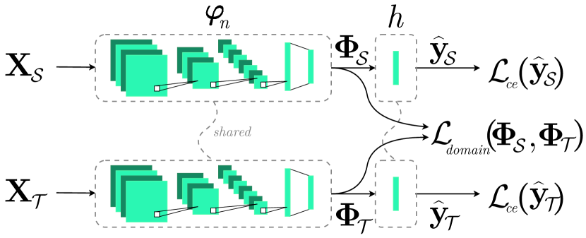
Two domains or two tasks are said to be different if their constituent parts are not the same. In some cases, the feature and label space of the source and target domains are equal. Then, the performance degradation associated with reusing a model in an unseen domain, is caused by a domain shift. The process of aligning the distributions between the domains is called Domain Adaptation. A special case of domain shift called covariate shift occurs when the difference between domains is caused by differences in their marginal input distributions [9], i.e. ). An efficient approach to Domain Adaptation in this case, is to use a deep neural network feature-extractor to transform the inputs of the respective domains into a common, domain-invariant space by means of a Siamese network architecture as seen in Fig. 1. A common classifier can then be trained on the latent features to make predictions on target domain data.
To align the domains with this approach, it is not strictly necessary to have labels available in the target dataset, and many Unsupervised Domain Adaptation methods can achieve good performance given enough (unlabelled) target data. In cases where the data is difficult to acquire, such as for medical images of a rare disease, Supervised Domain Adaptation methods are superior, and can utilise the few available target samples to efficiently align the domains. However, as we will show, having very few target data samples complicates the experiment design if best practices for train, validation, and test split independence are to be upheld. This few-shot supervised case is the focus of this work.
A typical optimisation goal in Supervised Domain Adaptation methods is to explicitly map samples belonging to the same class close together in a common latent subspace, while separating samples with different labels irrespective of the originating domain. In [10] it was shown that Graph Embedding [11], which aims at increasing the within-class compactness and between-class separability by appropriately connecting samples in intrinsic and penalty graph structures, provides a natural framework for Supervised Domain Adaptation, and produces results on par with the state-of-the-art. In this extension of [10], the following contributions are presented:
-
1.
We show that many existing Supervised Domain Adaptation methods aiming to produce a domain-invariant space by means of pairwise similarities can be expressed as Graph Embedding methods. Specifically, we analyse the loss functions of three recent state-of-the-art Supervised Domain Adaptation methods: Classification and Contrastive Semantic Alignment (CCSA) [6], Domain Adaptation using Stochastic Neighborhood Embedding (-SNE) [7], and Domain Adaptation with Neural Embedding Matching (NEM) [8].
-
2.
We argue that Graph Embedding and the specification of edges in the intrinsic and penalty graphs provides an expressive framework for encoding and exploiting assumptions about the datasets at hand.
-
3.
We identify flaws in the traditionally employed experiment protocol for Few-shot Supervised Domain Adaptation that violate machine learning best practices with regards to independence of train, validation and test splits.
-
4.
We propose a rectified experimental protocol, which clearly defines a validation set and ensures that the test set remains independent throughout experiments.
-
5.
We publish ready-to-use Python packages for the two most commonly used Few-shot Supervised Domain Adaptation datasets, Office31111Rectified Office31 splits: www.github.com/lukashedegaard/office31 and MNISTUSPS222Rectified MU splits: www.github.com/lukashedegaard/mnist-usps, which follow the rectified experimental protocol and are compatible with both Tensorflow and PyTorch through the use of a new open source library called Dataset Ops333Dataset Ops: https://github.com/lukashedegaard/datasetops.
- 6.
The remainder of the paper is structured as follows: In Section II, we provide a brief overview of Domain Adaptation methods that aim to find a domain-invariant latent space. We introduce Graph Embedding, how to optimise the graph preserving criterion, and multi-view extensions in Section III. Section IV delineates the Domain Adaptation via Graph Embedding (DAGE) framework and the DAGE-LDA method as proposed in [10]. In Section V, we analyse three recent state-of-the-art methods and show that they can also be viewed as Graph Embedding methods. In Section VI, we explain the issues with the existing experimental setup used in prior Domain Adaptation work and propose a rectified experimental protocol. Finally, in Section VII we present updated benchmark results on the canonical datasets Office-31, Digits and VisDA-C using the rectified protocol, and Section VIII draws the conclusions of the paper.
II Related Works
In Domain Adaptation (DA), it is usually assumed that all source data is labelled. Depending on the label availability for the target data, DA methods are categorised as Supervised, Semi-supervised, and Unsupervised. It is important to distinguish between these cases, as experiment protocols and the volume of data used for training varies widely between the three cases, even using the same datasets.
Supervised Domain Adaptation methods focus on few-shot learning scenarios, where the labelled target data is scarce with very few samples per class. Classification and Contrastive Semantic Alignment (CCSA) [6] is one such method, which embeds the contrastive loss introduced by Hadsell et al. [18] as a loss term in a two-stream deep neural network. Effectively, it places a penalty on the distance between samples with the the same class across source and target domains, as well as the proximity of samples that belong to different classes and fall within a distance margin. Domain Adaptation using Stochastic Neighborhood Embedding (-SNE) [7] uses the same deep two-stream architecture, and finds its inspiration in the dimensionality reduction method of Stochastic Neighbor Embedding (SNE). From it, a modified-Hausdorffian distance is derived, which minimises the Euclidean distance in the embedding space between the furthest same-class data pairs, and maximises the distance of the closest different-label pairs. Domain Adaptation With Neural Embedding Matching (NEM) [8] extends the contrastive loss of CCSA with an additional loss term to match the local neighbourhood relations of the target data prior to and after feature embedding. It does so with a graph embedding loss which connects the nearest neighbours of the target data in their original feature space and adds the weighted sum of distances between corresponding embedded features to the constrastive loss. In [19], an add-on domain classification layer is tasked with classifying the domain of training samples to produce a domain confusion loss that is used in feature extraction layers. Moreover, they take inspiration in distillation works, and use a soft label loss that matches a target sample to the average output distribution for the corresponding label in the source domain. Few-shot Adversarial Domain Adaptation (FADA) [20] uses a similar approach by training a domain-class discriminator with a four-way classification procedure for combinations of same- or different domain or class. In [21], an alignment loss for Second- or Higher-Order Scatter Tensors (So-HoT) is used to bring each within-class scatter closer in terms of their means and covariances. They do this by taking the squared norm of the difference between scatter tensors for each class.
Semi-supervised Domain Adaptation methods also have very few labelled target samples, but use unlabelled data in addition. Examples of this are -SNE and NEM, both of which provide extensions to include unlabelled data. In -SNE [7], the semi-supervised extension is achieved by a mechanism similar to the Mean-Teacher network technique [22], which entails the training of a parallel network on the unsupervised data and the use of an L2 consistency loss between the embeddings for the two networks. In NEM [8], a progressive learning strategy is employed, which gradually assigns pseudo labels to the most confident predictions on unlabelled data in each epoch. The pseudo-labelled data is then used for training in the next epoch. In graph-embedding based methods, such as DAGE-LDA [10], it is straight forward to incorporate unlabelled data into the loss by means of Label Propagation [23, 24]. Moreover, some unsupervised methods (e.g. [25, 26]) include semi-supervised extensions as well.
Unsupervised Domain Adaptation methods do not assume that any labels are available in the target domain, and use only the label information from the source domain. In Transfer Component Analysis (TCA) [27], domain are aligned by projecting data onto a set of learned transfer components. To learn the components, they minimise the Maximum Mean Discrepancy (MMD) in a Reproducing Kernel Hilbert Space (RKHS). In practice, the kernel trick is used to define a kernel matrix, and a projection matrix is learned from the corresponding empirical kernel map. Scatter Component Analysis (SCA) [28] also operates in a RKHS, but uses the notion of scatter (which recovers MMD) to align the domains. A projection matrix is then found by maximisation of the total- and between-class scatters, and minimisation of the domain- and within-class scatters. Here, between- and within-class scatters are defined only from source domain data. A recent addition to this space is the Graph Embedding Framework for Maximum Mean Discrepancy-Based Domain Adaptation Algorithm (GEF) [29], which assigns pseudo-labels to target data and solves the generalised eigenvalue problem for a MMD-based graph to compute a linear projection of the source data. The reconstructed source data is then used to train a classifier which in turn updates the psuedo-labels of the target data. In Locality Preserving Joint Transfer for Domain Adaptation (LPJT) [25], they use a multi-faceted approach of distribution matching to minimise the marginal- and conditional MMD: Landmark selection to learn importance weights for each source and target sample; label propagation, assigning pseudo labels to unlabelled samples; and locality preservation by use of Graph Embedding, solved as the generalised eigenvalue problem. Joint Distribution Invariant Projections (JDIP) [26] use a least-squares estimation of the distance for the joint distribution of source and target domains to produce mappings to a domain-invariant subspace with either linear or kernelized projections. Another branch of Unsupervised DA techniques use Adversarial methods to confuse the domains: In Domain-Adversarial Neural Networks (DANN) [16], a deep neural network is extended with an additional Discriminator head, that is trained to distinguish the source and target domains. This is similar to what was done in [19] for Supervised Domain Adaptation. Conditional Domain Adversarial Networks (CDAN) [30] take inspiration in the recent advances of Conditional Generative Adversarial Networks, and use multilinear- and entropy conditioning to improve discriminability and transferability between domains.
III Graph Embedding and its optimization problem
Graph Embedding [11] is a general dimensionality reduction framework based on the exploitation of graph structures. Suppose we have a data matrix and want to obtain its one-dimensional representation where . To encode the data relationships, which should be preserved in the subspace, we can construct a so-called intrinsic graph , where columns of the matrix represent vertices and elements in express the pair-wise relationships between these vertices. The element describes a non-negative edge weight between vertices and . When we want to suppress relationships between some graph vertices in the embedding space, we can create a corresponding penalty graph . The optimal one-dimensional embeddings are found by optimising the graph preserving criterion [11]:
| (1) |
where is a constant, and are graph Laplacian matrices of and , respectively, and and are the corresponding (diagonal) Degree matrices. Using a linear embedding, , the above criterion takes the form:
| (2) |
which is equivalent to maximizing the trace ratio problem [31, 32]:
| (3) |
Following Lagrange-based optimisation, the optimal projection is found by solving the generalized eigenanalysis problem and is given by the eigenvector corresponding to the maximal eigenvalue.
When , the trace ratio problem in Eq. (3) becomes:
| (4) |
where is the trace operator and is a projection matrix. The trace ratio problem in Eq. (4) does not have a closed-form solution. Therefore, it is conventionally approximated by solving the ratio trace problem, . The ratio trace problem can be reformulated as the generalised eigenvalue problem via a Lagrangian formulation, so the problem is reduced to finding the vector that satisfies for . The columns of are given by the eigenvectors of the matrix corresponding to the maximal eigenvalues. The trace ratio problem in Eq. 3 can also be converted to an equivalent trace difference problem [31]:
| (5) |
where is the trace ratio calculated by applying an iterative process as described in [31] and [33]. After obtaining the trace ratio value , the optimal projection matrix is obtained by substitution of into the trace difference problem in Eq. (5) and maximisation of its value.
Non-linear mappings from to can be obtained by exploiting the Representer Theorem, i.e. by use of an implicit nonlinear mapping , with a reproducing kernel space, leading to . We can express the mapping in the form of where are the training data representations in and the projection matrix is given by . In that case, the problems in Eqs. (4) and (5) are transformed by substituting with , which is the kernel matrix calculated using the kernel function .
Extensions which use intrinsic and penalty graphs to jointly determine transformations for data from multiple input spaces (views) have also been proposed. As was shown in [34], several such methods (called multi-view methods), including Multi-View Fisher Discriminant Analysis [35], Partial Least Squares [36], (deep) Canonical Correlation Analysis [37], and Multi-view Discriminant Analysis [38] can be expressed as specific instantiations of the problem in Eq. 4, which exploit the view label information to define corresponding intrinsic and penalty graphs. Moreover, the Multi-view Nonparametric Discriminant Analysis [39] and Deep Multi-view Learning to Rank [40] methods have been formulated based on the problem in Eq. 4 for retrieval and ranking problems.
IV Domain Adaptation via Graph Embedding
Given the versatility of graph embedding, we derive the framework for Domain Adaptation via Graph Embedding (DAGE) in this section, and detail a simple yet effective instantiation inspired by Linear Discriminant Analysis.
IV-A DAGE Framework
The aim of transformation-based Domain Adaptation methods is to learn a common subspace where the distribution gap between source domain data and target domain data is as small as possible. In the supervised setting, we want a transformation , which places samples of the same class close together without regard to the originating domain to achieve within-class compactness. On the other hand, we want to clearly separate samples with different labels irrespective of the domain to gain between-class separability.
Let and be two data matrices from the source and target domains, respectively, and let . Suppose we have a transformation which can produce -dimensional vectors from -dimensional data. Then we can construct a matrix containing the transformed data from both domains. By encoding the desired pair-wise data relationships in an intrinsic graph and computing its graph Laplacian matrix , we can formulate a measure of within-class spread as
| (6) |
Similarly, we can create a penalty graph and express the between-class separability using
| (7) |
Since the goal is to minimise the within-class spread (Eq. 6) and maximise the between-class separability (Eq. 7), we can utilise the trace ratio objective function to perform Domain Adaptation via Graph Embedding:
| (8) |
Note that the graph Laplacian matrices of the intrinsic and the penalty graphs are placed respectively in the numerator and denominator of the trace ratio problem, since Eq. 8 corresponds to a minimization problem. Note also that the criterion in Eq. 8 can be seen as the multidimensional generalisation of Eq. 1 in which an arbitrary function is used in place of a linear projection .
When the transformation is a linear projection , i.e. , the DAGE criterion becomes:
| (9) |
where . The optimal transformation matrix is obtained by solving the ratio trace problem. Its solution is formed by the eigenvectors corresponding to the largest eigenvalues of the generalised eigenvalue problem , or by minimising the trace difference problem as described in Section III:
| (10) |
The linear DAGE criterion in Eq. 9 can also be formulated using the kernel trick for non-linear mappings. Suppose is a nonlinear function mapping the input data into a reproducing kernel Hilbert space . Let the matrix be composed of data in . Based on the Representer Theorem, we let and get
| (11) |
where has elements equal to . The solution of Eq. 11 can be found via generalised eigenvalue decomposition or by applying an iterative process similar to the linear case.
Eigenvalue decomposition for nonlinear DAGE is intractable for large datasets as the computational complexity is in the order of [41]. An alternative solution is to express the DAGE criterion as part of the loss function in a deep neural network. For Supervised Domain Adaptation problems in the visual domain, the first layers of a neural network architecture can be seen as a non-linear parametric function taking as input the raw image data and giving vector representations as output. This allows the DAGE objective to be optimised with gradient descent-based approaches. Moreover, the DAGE loss can be optimised together with a classification loss (e.g. cross-entropy) in an end-to-end manner. Given a mini-batch of data, the DAGE loss can be computed:
| (12) |
where is a matrix formed by the transformed features in the mini-batch and the graph Laplacian matrices and are computed on the data forming the mini-batch. Optimisation using batches is also applied commonly in dimensionality reduction methods when the full data does not fit in memory [42, 43, 44]. The gradient for a mini-batch is:
| (13) |
The resulting loss to be optimised is the sum of the DAGE loss and classification losses for source and target domain data:
| (14) |
where and denote the parameters of the parametric functions for feature extraction and for classification, respectively. are mixing coefficients for the ratio of domain adaptation to cross entropy losses and ratio of source and target cross entropy losses.
[H] Procedure for training a DAGE-LDA model {algorithmic}[1] \REQUIRESource data , target data , number of training epochs , hyper-parameters () \ENSURETrained neural network model \STATE Load pre-trained network weights (FT-Source) \FOR in epochs \STATESplit dataset into training, validation and test sets according to the rectified experiment protocol. \FOReach mini-batch in training set \STATE \STATECreate , e.g. from Eq. 15 using mini-batch . \STATECreate , e.g. from Eq. 16 using mini-batch . \STATECompute according to Eq. 12. \STATEUpdate by optimising Eq. 14 via gradient descent on mini-batch . \ENDFOR\ENDFOR
IV-B DAGE-LDA
The DAGE criterion in Eq. 8 is a generic criterion which can lead to a multitude of Domain Adaptation solutions. Constructing the two graphs and in different ways gives rise to different properties to be optimised in the subspace . A simple instantiation of DAGE inspired by Linear Discriminant Analysis is obtained by using an intrinsic graph structure that connects samples of the same class:
| (15) |
where and are the labels associated with the -th and -th samples, respectively. The corresponding penalty graph structure connects samples of different classes:
| (16) |
Despite the simplicity of the above-described DAGE instantiation, the method produces state-of-the-art results as will be shown in Section VII.
V State of the Art Supervised Domain Adaptation Methods perform Graph Embedding
In Section IV, we analysed the domain-invariant space approach to Supervised Domain Adaptation, and showed that it can be naturally described as multi-view Graph Embedding. In fact, any domain adaptation method, which uses pairs of samples to produce a domain-invariant latent space, can be cast as a multi-view Graph Embedding method. To illustrate this point, we analyse three recent state-of-the-art methods and show that they are instances of Domain Adaptation via Graph Embedding with different choices of and . A similar relationship can be shown for several other Domain Adaptation methods such as [45, 21]. In the subsequent subsections, we focus on the Domain Adaptation terms included in the optimisation function of each method, while we omit the corresponding cross-entropy terms of each method for simplicity.
V-A Classification and Contrastive Semantic Alignment
The contrastive semantic alignment loss of CCSA [6] is constructed from two terms: A similarity loss , which penalises the distance between within-class samples of different domains, and a dissimilarity loss , which penalises the proximity of between-class samples if they come within a distance margin , i.e.:
| (17) |
Using as notational shorthand , the partial losses are defined as follows:
| (18) | ||||
| (19) |
The similarity loss can be expressed equivalently in terms of the weighted summation over graph edges:
| (20) |
where the graph weight matrix has an edge for sample-pairs with the same label but different originating domains
| (21) |
and is the graph Laplacian matrix associated with . Using the fact that , the dissimilarity loss can likewise be expressed in terms of a summation over graph edges:
| (22) |
where
| (23) |
and is the graph Laplacian matrix associated with the corresponding weight matrix . Note that the weight matrix of Eq. 23 constitutes an -distance margin rule for graph embedding. The partial similarity and dissimilarity losses can thus be expressed with graph Laplacian matrices which encode the within-class and between-class relations. Combining Eqs. (20) and (V-A), we see that the contrastive semantic alignment loss of CCSA is equivalent to:
| (24) |
which constitutes the trace difference problem in Eq. (10) from Graph Embedding. While CCSA employs a value of , one can also determine an optimised value for .
V-B Domain Adaptation using Stochastic Neighborhood Embedding
Following the procedure outlined above, it is straightforward to show that -SNE [7] can also be viewed as a graph embedding. For each target sample, the domain adaptation loss term of -SNE penalises the furthest distance to a within-class source sample, and encourages the distance for the closest between-class to source sample to be maximised:
| (25) |
We can readily express this using the trace difference formulation:
| (26) |
with and Graph Laplacian matrices and corresponding to the weight matrices:
| (27) | ||||
| (28) |
Because only a single edge is specified for each source sample per graph Laplacian, it is worth noting that the resulting graph connectivity for -SNE is highly dependent on the batch size used during optimisation. Small batch sizes will result in more densely connected graphs than large batch sizes.
V-C Neural Embedding Matching
NEM [8] extends the contrastive loss of CCSA with an additional term designed to maintain the neighbour relationship of target data throughout the feature embedding:
| (29) |
Here, the hyperparameter weights the importance of the neighbour matching loss, which is specified as the loss over a neighbourhood graph with edges between each target sample and its nearest neighbours in the original feature space:
| (30) |
where is the Radial Basis Function kernel used to assign a weight to the edge between any pair of vertices. To express the NEM loss in terms of a graph embedding, the neighbour term can be incorporated into the similarity weight matrix by extending the encoding rule from Eq. 21:
| (31) |
The penalty weight matrix for NEM is the same as for CCSA in Eq. 23 and the final graph embedding problem is a trace difference problem as in Eqs. (24) and (26).
V-D Discussion
While some methods [28, 29, 10] explicitly formulate the process of Domain Adaptation as Graph Embedding, we have shown that many others [6, 7, 8], which employ pairwise (dis)similarities between data, can also be formulated as such. It would be trivial to perform the same analysis on other methods (e.g [21]).
Of course, not all Domain Adaptation methods fit nicely into the structure of Graph Embedding. The use of an adversarial network branch [19, 16, 30] is not straight-forward to integrate into the intrinsic and penalty matrices of a Graph Embedding. Moreover, progressive learning strategies and the use of pseudo-labels in semi- and unsupervised methods [8, 29] relates more to the training loop than the loss-formulation. Nonetheless, Graph Embedding captures many existing powerful Domain Adaptation methods, and gives us a common lens through which to see them: In CCSA, all same-class sample pairs are given a similar attraction, while different-class pairs are only repelled if they come within a distance margin; in NEM, target domain samples are additionally encouraged to remain close if they were similar in their input-space; in -SNE, for each sample only the furthest same-class sample is attracted, while the closest sample of different label is repelled; in DAGE-LDA, we simply attract same-class pairs and repel different-class pairs without further assumptions.
An ongoing challenge in Machine Learning and Domain Adaptation is how to clearly encode our prior knowledge and assumptions into the learning problem for a specific application [9]. We would argue that the construction rules for the graph Laplacian matrices of Graph Embedding may be an ideal way to specify this in a simple if-then-else manner. Say, we want to encode an assumption that some classes (e.g. bike and bookcase) have large within-class differences, while others to not. In the intrinsic matrix, we might then state a rule, that the bike and bookcase classes should only attract the most similar same-class sample and ignore the others, while all samples should be attracted equally for the other classes. The is a plethora of options for constructing the graphs using margins, nearest-neighbour rules, etc. We leave thier exploration to future work.
VI Rectified Experimental Protocol for Few-shot Supervised Domain Adaptation
An important aspect of conducting experiments on domain adaptation in few-shot settings relates to how the data should be split. In this section, we describe the experimental setup that is normally used to evaluate and compare supervised Domain Adaptation methods. We showcase issues related to non-exclusive use of data in model selection and testing phases and we describe how the evaluation process can be improved by proposing a new experimental setup.
VI-A Traditional Experiment Setup
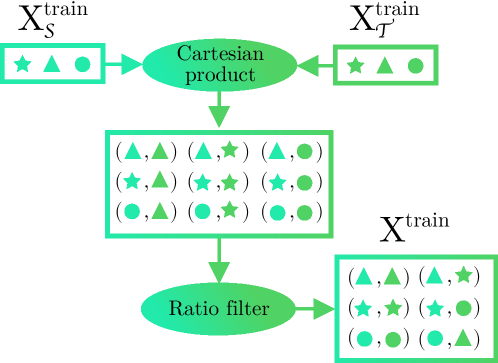
The experiment setup used to evaluate the performance of Domain Adaptation methods, e.g. [6, 7], is as follows: A number of samples of each class are drawn from the source domain, and a few samples per class are drawn from the target domain to be used for training. For instance, in experiments on the Office31 dataset [12] with the Amazon data as source domain and the Webcam data as target domain, the number of samples per class forming the training set is equal to twenty and three, respectively. The remaining target data is used for testing. The sampled data from both source and target domains are paired up as the Cartesian product of the two sets, producing as the resulting dataset all combinations of two samples from either domain. To limit the size and redundancy, the dataset is filtered to have a predefined ratio of same-class samples (where both samples in a pair have the same label) to different-class samples. This ratio is commonly set equal to 1:3. An illustration of this is found in Fig. 2.
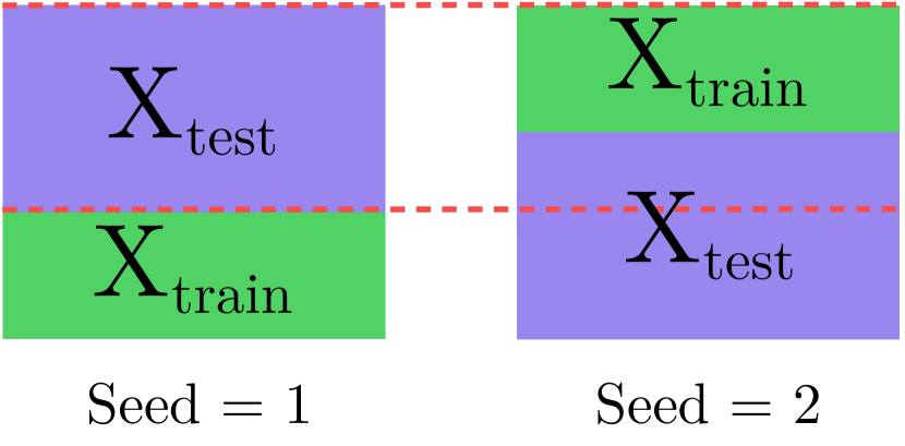
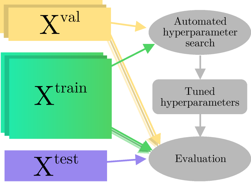
This combined dataset is then used to train a model with a Domain Adaptation technique, e.g. using the two stream architecture as illustrated in Fig. 1. The final evaluation is conducted on the test set from the target domain. Because very few unique samples from the target domain are used for training in each experiment, the results will usually vary significantly between runs and will depend on the random seed used for creating the training and test splits. Therefore, each experiment is repeated multiple times, each time with a new seed value, and the mean accuracy alongside the standard deviation over the runs are reported. The absence of validation data on each experiment has the risk of performing model selection (including hyper-parameter search) based on the performance on the test data. One could try to avoid the problem by performing model selection and hyper-parameter search using training/test splits from seed values which are not used for the final training/test splits. This, however, is not enough to guarantee that the test performance generalises to unseen data, since it is probable that test data is used for model selection and hyper-parameter search, as illustrated in Fig. 3.
VI-B Rectified Experiment Setup
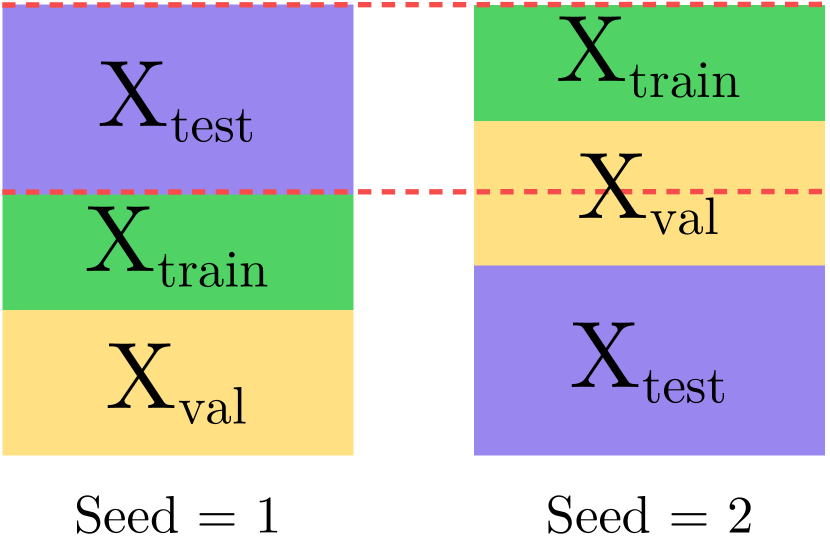
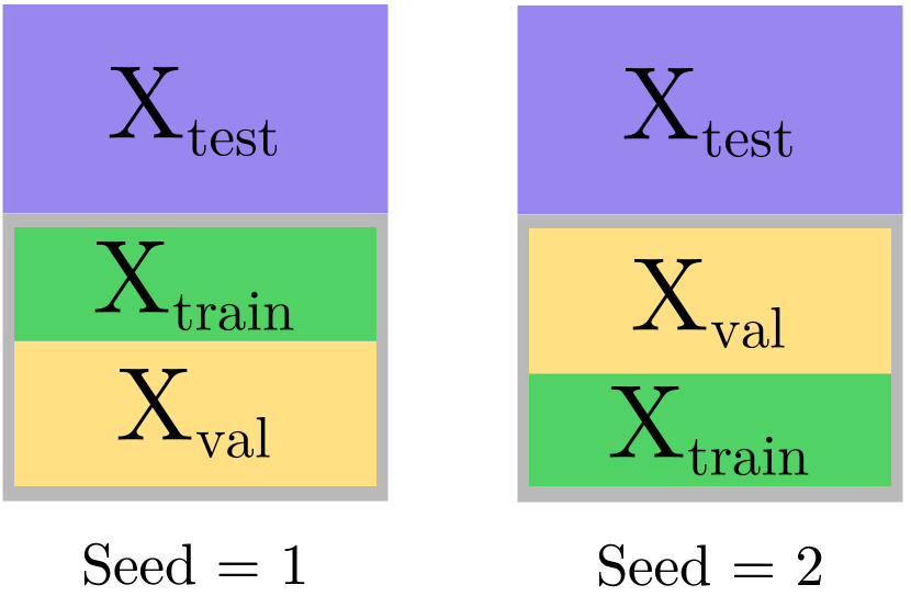
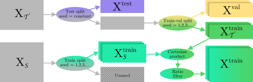
To avoid the above described issues of the experiment setup used in evaluating the performance of Domain Adaptation methods, we need to conduct our sampling in two steps: First, we need to define the data in the target domain that will be used for evaluating the performance of the Domain Adaptation method in all the runs. The remaining data in the target domain will be used to form the training and validation sets in the target domain in different runs. This can be done exactly as described in Section VI-A: We draw few samples from the source domain and the training set of the target domain, and combine them using the Cartesian Product with an optional ratio for filtering. In this way, we ensure that independent test data is used for method evaluation, and a validation set is available for model selection and hyper-parameter search. This data splitting procedure is illustrated in Fig. 4(a).
| Experiment setup | Traditional [10] | Rectified | Difference |
|---|---|---|---|
| CCSA | 83.1 | 82.2 | - 0.9 |
| d-SNE | 83.6 | 81.6 | - 2.0 |
| DAGE-LDA | 83.6 | 82.8 | - 0.8 |
| Average | - 1.2 |
VII Experiments and Results
In this section, we conduct experiments on the Office31, Digits (MNIST, USPS, SVHN, MNIST-M), and VisDA datasets using the rectified experimental setup and compare the results to those from the traditional experimental setup.
VII-A Datasets
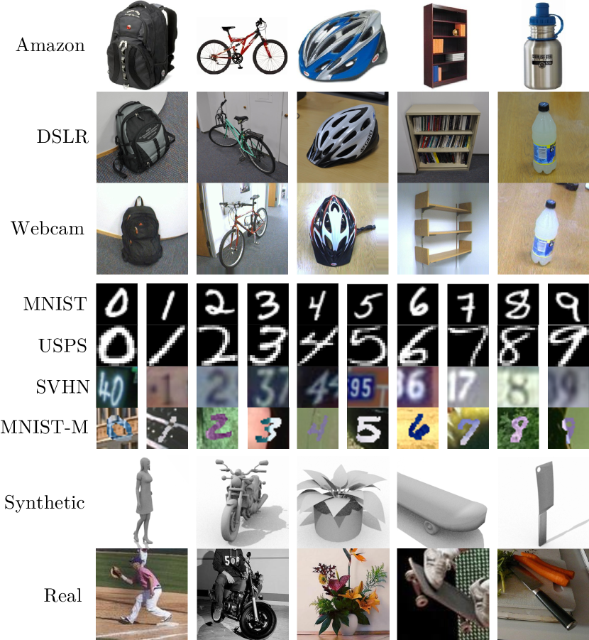
The Office31 dataset [12] contains images of 31 object classes found in the modern office. It has three visual domains: Amazon () consists of 2.817 images found on the e-commerce site www.amazon.com. These images are generally characterised by their white background and studio-lighting conditions. DSLR () contains 498 high resolution images taken using a digital single-lens reflex camera. Webcam () has 795 images captured using a web-camera. The objects photographed are the same as for DSLR, but the images in this case are low-resolution and suffer from visual artefacts such as colour imbalances and optical distortion. A sample of the Office31 images is shown in Fig. 5.
The digits datasets contain handwritten digits from 0 to 9 and comprise MNIST [13], USPS [14], SVHN [15], and MNIST-M [16]. MNIST consists of 70,000 grayscale images with a resolution, USPS has 11,000 grayscale images, SVHN has 99,280 RGB images of house numbers, and MNIST-M is a dataset generated by superimposing RGB backgrounds on MNIST.
VisDA-2017 [17] is a large-scale Domain Adaptation dataset comprising three domains with 12 common object cateogies. The domains comprise a training (source) domain of synthetic 3D object renderings, as well as validation and test domains (targets) with real images from the MS COCO [46] and YouTube-BoundingBoxes [47] datasets respectively.
§Only relevant for CCSA and -SNE. ¶Only relevant for the experiments in Office31 dataset.
VII-B Office31
In our experiments on the Office31 dataset, we used a model consisting of the convolutional layers of a VGG-16 [48] network pretrained on ImageNet [49] with randomly initialised dense layers of 1024 and 128 neurons, respectively, as done in [6, 7]. This network is subsequently fine-tuned on all source data (FT-Source). We found a gradual-unfreeze procedure [50], where four pretrained layers are unfrozen each time the model converges, to work well. To produce a baseline method (FT-Target), the FT-Source model is further fine-tuned on the target data.
We follow the experimental procedure described in Section VI-B. After first splitting off 30% of the target data to form the test set, we create the training set using twenty source samples per class for the Amazon domain, and eight source samples per class for DSLR and Webcam. From the target domain, three samples per class are drawn in each case. The remaining target data is used as a validation set. Thus, we employ the same number of samples for training as in the traditional split [19, 7, 6], but ensure an independent test split as well as a well-defined validation split. The model is duplicated across two streams with shared weights as depicted in Fig. 1 and trained on the combined training data, with one domain entering each stream. This experiment is performed for all six combinations of source and target domain in , and each combination is run five times using different seeds. We re-implemented CCSA and -SNE using their publicly available source code and included them in our experiments. Prior to executing the five runs, an independent hyper-parameter search on the space summarised in LABEL:tab:search-space was conducted for each method using Bayesian Optimisation with the Expected Improvement acquisition function [51] given 100 trials. For the final tests, we used data augmentation with random modifications of colour hue and saturation, image brightness and contrast, as well as rotation and zoom. For a fair comparison, all hyper-parameter tuning and tests are performed with the exact same computational budget and data available for all methods tested.
The best performing hyper-parameter values are used to train the model following a standard procedure. The training procedure for DAGE-LDA is described in Section IV-A. Once a model is trained, we use the test data to generate predictions and report the macro average classification accuracy.
The results for Office31 are shown in Section VI-B and Table II. Comparing the CCSA and -SNE results of the traditional experimental setup with the rectified one, we see that the achieved macro accuracy is generally lower: on average for CCSA, -SNE and DAGE-LDA. This is in-line with our expectations, and confirms that the traditional setup may have suffered from generalisation issues as described in Section VI-A. Comparing CCSA, -SNE, and DAGE-LDA in the rectified experimental setup, we see that DAGE-LDA has the highest average score across all six adaptations, though it only outperforms the other methods on a single adaptation (). CCSA performs next best, and -SNE comes last of the three. This suggests, that the higher accuracy reported in [7] as compared to [6] may be due to better hyper-parameter optimisation rather than a better Domain Adaptation loss.
As an additional experiment, we repeat the adaptation task for DAGE-LDA using the ResNet-50 [52] to gauge the effect of using an improved feature-extractor. Comparing the VGG-16 results with those for ResNet-50, we observe an average improvement of . This matches the relative difference in top-1 accuracy on ImageNet ( for VGG16 and for ResNet-50 [52]), and highlights the importance of disclosing which feature-extractor is used in derived methods [53].
VII-C Digits
For our experiments on the digits datasets MNIST, USPS, SVHN, and MNIST-M, we use a network architecture which has two streams with shared weights, with two convolutional layers containing 6 and 16 filters respectively, max-pooling, and two dense layers of size 120 and 84 prior to the classification layer. This architecture is the same as the one used in [6]. The test-train splits were predifined from TorchVision Datasets [54] and TensorFlow Datasets [55], and validation data was sampled from the train split of the target dataset. Though our implementation uses Tensorflow, the datasets were made compatible using the Dataset Ops library. Aside from following the rectified sampling, the experiments use the procedures from [56, 6, 7]. For augmentations, zoom, brightness and contrast perturbations, as well as colour saturation and hue augmentations were applied when relevant.
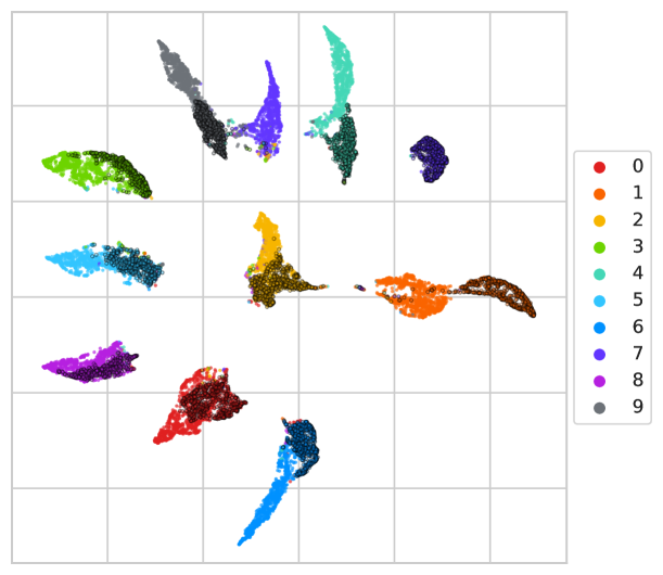
The first set of experiments on the digits datasets are the transfers between MNIST and USPS, MNIST and SVHN, and from MNIST to MNIST-M. Here, we sample 10 samples per class from the target train split, and use 5,000 randomly sampled images per class for MNIST and 700 per class for USPS and SVHN. The experiments are repeated 5 times. Prior to this, a hyper-parameter search using Bayesian Optimisation and the search space described in LABEL:tab:search-space was conducted for the MNISTUSPS task. These hyper-parameters were used for the remaining transfers, except for the MNISTSVHN transfer, which had its own hyper-parameter search using an equivalent computational budget for each method. The results are presented in Table IV. Here, DAGE-LDA has the highest accuracy on most tasks, with CCSA and d-SNE achieving slightly higher accuracy on one transfer each. A 2D UMAP [57] visualisation of the latent space features produced using the DAGE-LDA loss in the USPSMNIST adaptation is shown in Fig. 6.
The second set of experiments consider a few-shot transfer, were the network is trained from random initialisation using 2,000 randomly sampled images per class from MNIST (source) and a varying number of USPS (target) samples per class. Experiments with 1, 3, 5 and 7 target samples per class were conducted and each experiment was repeated 10 times. The results obtained by running the experiments are shown in Table V. Comparing CCSA, -SNE and DAGE-LDA, we find that DAGE-LDA has the highest average accuracy, closely followed by CCSA and then -SNE. While the originally reported results for -SNE [7] show better performance than the other methods, it should be noted they used a LeNet [58] architecture for feature extraction. Based on our own results for -SNE, which used a CNN-architecture similar to the other methods, we attribute their higher accuracy to the choice of feature-extractor.
VII-D VisDA Classification
Following the setup in [7], the VisDA-C experiments use a ResNet-152V2 model as classification backbone. First, it is loaded with ImageNet-pretrained weights and finetuned on the synthetic source data. These model weights subsequently initialise the SDA methods, which employ 10 samples per class from the target domain (real) in addition to 100 samples per class from the source data (synthetic) for training and 30% for validation. The evaluation results on the remaining target data is shown in Section VII-D.
| Method | Traditional [7] | Rectified (ours) |
|---|---|---|
| FT-Source | 52.8 | 54.5 |
| \cdashline1-3 CCSA | 76.9 | |
| d-SNE | 80.7 | |
| DAGE-LDA | - |
VII-E Sensitivity Analysis
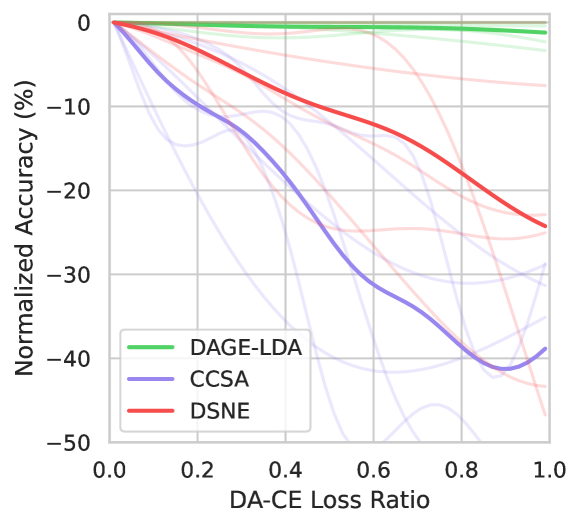
A result of Bayesian Optimisation is a statistical model, which gives an expected optimisation value (accuracy) and confidence bounds for any hyper-parameter combination within the search space. To gauge the sensitivity of the domain adaptation loss weightings, we use the Bayesian model to compute the partial dependence of each hyper-parameter. The partial dependence “averages out” the influence of other hyper-parameters, and yields the best estimate given the 100 trials performed during hyper-parameter optimisation of Office31 transfers. Because the Bayesian optimisation chooses trials sequentially in a trade-off between exploration and exploitation, it should be noted that the estimate for high performing hyper-parameter values have tighter confidence bounds than low performers. In Fig. 7, we see plots of the average estimates of normalised accuracy for the ratio of domain adaptation loss to cross entropy loss, , as defined in Eq. 14.
We observe that CCSA and -SNE are highly sensitive to the chosen value of . For these methods, the domain adaptation loss works best when used as a regularisation term of small magnitude, and high values may lead to divergence during training. Meanwhile, DAGE-LDA works well over a range of chosen values. This makes sense, considering that the DAGE-LDA criterion explicitly minimises within-class distances and maximises between-class distances, which is akin to the operation performed by cross entropy for categorical data.
VIII Conclusion
In this paper, we have shown that Domain Adaptation can be viewed as Graph Embedding (DAGE) and that many existing methods for Supervised Domain Adaptation (SDA) can be formulated in this common framework. Within the DAGE framework, a very simple LDA-inspired instantiation matches or surpasses the current state-of-the-art methods on few-shot supervised adaptation task using the standard benchmarks in SDA. Moreover, we argued that the intrinsic and penalty graph Laplacian matrices in Graph Embedding give us a straight-forward way of encoding application-specific assumptions about the domain and tasks at hand. Finally, we highlighted some generalisation and reproducibility issues related to the experimental setup commonly used to evaluate the performance of Domain Adaptation methods and proposed a rectified experimental setup for more accurately assessing and comparing the generalisation capability of SDA methods. Alongside our source code, we made the revised training-validation-test splits available to facilitate fair comparisons of SDA methods in future research.
Acknowledgement
Lukas Hedegaard and Alexandros Iosifidis acknowledge funding from the European Union’s Horizon 2020 research and innovation programme under grant agreement No 871449 (OpenDR). Omar Ali Sheikh-Omar was partially funded from Innovation Fund Denmark under grant agreement No 0153-00233A.
References
- Arpit et al. [2017] D. Arpit, S. Jastrzebski, N. Ballas, D. Krueger, E. Bengio, M. S. Kanwal, T. Maharaj, A. Fischer, A. Courville, Y. Bengio et al., “A closer look at memorization in deep networks,” in International Conference on Machine Learning, 2017, pp. 233–242.
- Pan and Yang [2010] S. J. Pan and Q. Yang, “A survey on transfer learning,” IEEE Transactions on Knowledge and Data Engineering, vol. 22, no. 10, pp. 1345–1359, 2010.
- Weiss et al. [2016] K. Weiss, T. M. Khoshgoftaar, and D. Wang, “A survey of transfer learning,” Journal of Big data, vol. 3, no. 1, p. 9, 2016.
- Torrey and Shavlik [2010] L. Torrey and J. Shavlik, “Transfer learning,” in Handbook of Research on Machine Learning Applications and Trends: Algorithms, Methods, and Techniques, 2010, pp. 242–264.
- Raitoharju et al. [2016] J. Raitoharju, E. Riabchenko, K. Meissner, I. Ahmad, A. Iosifidis, M. Gabbouj, and S. Kiranyaz, “Data enrichment in fine-grained classification of aquatic macroinvertebrates,” in ICPR 2nd Workshop on Computer Vision for Analysis of Underwater Imagery, 2016, pp. 43–48.
- Motiian et al. [2017a] S. Motiian, M. Piccirilli, D. A. Adjeroh, and G. Doretto, “Unified deep supervised domain adaptation and generalization,” in IEEE International Conference on Computer Vision, 2017, pp. 5715–5725.
- Zhou et al. [2020] X. Zhou, X. Xu, R. Venkatesan, G. Swaminathan, and O. Majumder, “d-sne: Domain adaptation using stochastic neighborhood embedding,” Domain Adaptation in Computer Vision with Deep Learning, pp. 43–56, 2020.
- Wang et al. [2019] Z. Wang, B. Du, and Y. Guo, “Domain adaptation with neural embedding matching,” IEEE Transactions on Neural Networks and Learning Systems, pp. 1–11, 2019.
- Kouw and Loog [2018] W. M. Kouw and M. Loog, “An introduction to domain adaptation and transfer learning,” preprint, arXiv:1812.11806, 2018.
- Hedegaard et al. [2021] L. Hedegaard, O. A. Sheikh-Omar, and A. Iosifidis, “Supervised domain adaptation using graph embedding,” International Conference on Pattern Recognition, 2021.
- Yan et al. [2006] S. Yan, D. Xu, B. Zhang, H.-J. Zhang, Q. Yang, and S. Lin, “Graph embedding and extensions: A general framework for dimensionality reduction,” IEEE Transactions on Pattern Analysis and Machine Intelligence, vol. 29, no. 1, pp. 40–51, 2006.
- Saenko et al. [2010] K. Saenko, B. Kulis, M. Fritz, and T. Darrell, “Adapting visual category models to new domains,” in European Conference on Computer Vision, 2010, pp. 213–226.
- Lecun et al. [1998] Y. Lecun, L. Bottou, Y. Bengio, and P. Haffner, “Gradient-based learning applied to document recognition,” in Proceedings of the IEEE, 1998, pp. 2278–2324.
- LeCun et al. [1990] Y. LeCun, B. E. Boser, J. S. Denker, D. Henderson, R. E. Howard, W. E. Hubbard, and L. D. Jackel, “Handwritten digit recognition with a back-propagation network,” in Advances in Neural Information Processing Systems 2, 1990, pp. 396–404.
- Netzer et al. [2011] Y. Netzer, T. Wang, A. Coates, A. Bissacco, B. Wu, and A. Y. Ng, “Reading digits in natural images with unsupervised feature learning,” in NIPS Workshop on Deep Learning and Unsupervised Feature Learning 2011, 2011.
- Ganin et al. [2016] Y. Ganin, E. Ustinova, H. Ajakan, P. Germain, H. Larochelle, F. Laviolette, M. March, and V. Lempitsky, “Domain-adversarial training of neural networks,” Journal of Machine Learning Research, vol. 17, no. 59, pp. 1–35, 2016.
- Peng et al. [2018] X. Peng, B. Usman, N. Kaushik, D. Wang, J. Hoffman, and K. Saenko, “Visda: A synthetic-to-real benchmark for visual domain adaptation,” in IEEE Conference on Computer Vision and Pattern Recognition Workshops, June 2018.
- Hadsell et al. [2006] R. Hadsell, S. Chopra, and Y. LeCun, “Dimensionality reduction by learning an invariant mapping,” in IEEE Conference on Computer Vision and Pattern Recognition, vol. 2, 2006, pp. 1735–1742.
- Tzeng et al. [2015] E. Tzeng, J. Hoffman, T. Darrell, and K. Saenko, “Simultaneous deep transfer across domains and tasks,” in IEEE International Conference on Computer Vision, 2015, pp. 4068–4076.
- Motiian et al. [2017b] S. Motiian, Q. Jones, S. Iranmanesh, and G. Doretto, “Few-shot adversarial domain adaptation,” in Advances in Neural Information Processing Systems, 2017, vol. 30, pp. 6670–6680.
- Koniusz et al. [2017] P. Koniusz, Y. Tas, and F. Porikli, “Domain adaptation by mixture of alignments of second-or higher-order scatter tensors,” in IEEE Conference on Computer Vision and Pattern Recognition, 2017, pp. 7139–7148.
- Tarvainen and Valpola [2017] A. Tarvainen and H. Valpola, “Mean teachers are better role models: Weight-averaged consistency targets improve semi-supervised deep learning results,” in Advances in Neural Information Processing Systems, 2017, vol. 30, pp. 1195–1204.
- Zhu et al. [2003] X. Zhu, Z. Ghahramani, and J. Lafferty, “Semi-supervised learning using gaussian fields and harmonic functions,” in International Conference on Machine Learning, 2003, p. 912–919.
- Weston et al. [2008] J. Weston, F. Ratle, and R. Collobert, “Deep learning via semi-supervised embedding,” in International Conference on Machine Learning, 2008, p. 1168–1175.
- Li et al. [2019] J. Li, M. Jing, K. Lu, L. Zhu, and H. T. Shen, “Locality preserving joint transfer for domain adaptation,” IEEE Transactions on Image Processing, vol. 28, no. 12, pp. 6103–6115, 2019.
- Chen et al. [2020a] S. Chen, M. Harandi, X. Jin, and X. Yang, “Domain adaptation by joint distribution invariant projections,” IEEE Transactions on Image Processing, vol. 29, pp. 8264–8277, 2020.
- Pan et al. [2011] S. J. Pan, I. W. Tsang, J. T. Kwok, and Q. Yang, “Domain adaptation via transfer component analysis,” IEEE Transactions on Neural Networks, vol. 22, no. 2, pp. 199–210, 2011.
- Ghifary et al. [2017] M. Ghifary, D. Balduzzi, W. B. Kleijn, and M. Zhang, “Scatter component analysis: A unified framework for domain adaptation and domain generalization,” IEEE Transactions on Pattern Analysis and Machine Intelligence, vol. 39, no. 7, pp. 1414–1430, 2017.
- Chen et al. [2020b] Y. Chen, S. Song, S. Li, and C. Wu, “A graph embedding framework for maximum mean discrepancy-based domain adaptation algorithms,” IEEE Transactions on Image Processing, vol. 29, pp. 199–213, 2020.
- Long et al. [2018] M. Long, Z. Cao, J. Wang, and M. I. Jordan, “Conditional adversarial domain adaptation,” in Advances in Neural Information Processing Systems, 2018, vol. 31, pp. 1640–1650.
- Jia et al. [2009] Y. Jia, F. Nie, and C. Zhang, “Trace ratio problem revisited,” IEEE Transactions on Neural Networks, vol. 20, no. 4, pp. 729–735, 2009.
- Iosifidis et al. [2013] A. Iosifidis, A. Tefas, and I. Pitas, “On the optimal class representation in linear discriminant analysis,” IEEE Transactions on Neural Networks and Learning Systems, vol. 24, no. 9, pp. 1491–1497, 2013.
- Guo et al. [2003] Y.-F. Guo, S.-J. Li, J.-Y. Yang, T.-T. Shu, and L.-D. Wu, “A generalized foley–sammon transform based on generalized fisher discriminant criterion and its application to face recognition,” Pattern Recognition Letters, vol. 24, no. 1-3, pp. 147–158, 2003.
- Cao et al. [2018] G. Cao, A. Iosifidis, and M. Gabbouj, “Generalized multi-view embedding for visual recognition and cross-modal retrieval,” IEEE Transactions on Cybernetics, vol. 48, no. 9, pp. 2542–2555, 2018.
- Diethe et al. [2008] T. Diethe, D. Hardoon, and J. Shawe-Taylor, “Multiview fsher discriminant analysis,” in Neural Information Processing Systems, 2008.
- Wold et al. [1984] S. Wold, A. Ruhe, H. Wold, and W. Dunn, “The collinearity problem in linear regression: The partial least squares (pls) approach to generalized inverses,” SIAM Journal on Scientific and Statistical Computing, vol. 5, no. 3, pp. 735–743, 1984.
- Andrew et al. [2013] G. Andrew, R. Arona, J. Bilmes, and K. Livescu, “Deep canonical correlation analysis,” in International Conference on Machine Learning, 2013, pp. 1247–1255.
- Kan et al. [2016] M. Kan, S. Shan, H. Zhang, S. Lao, and X. Chen, “Multi-view discriminant analysis,” IEEE Transactions on Pattern Analysis and Machine Intelligence, vol. 38, no. 1, pp. 188–194, 2016.
- Cao et al. [2017] G. Cao, A. Iosifidis, and Gabbouj, “Multi-view nonparametric discriminant analysis for image retrieval and recognition,” IEEE Signal Processing Letters, vol. 24, no. 10, pp. 1537–1541, 2017.
- Cao et al. [2021] G. Cao, A. Iosifidis, M. Gabbouj, V. Raghavan, and R. Gottumukkala, “Deep multi-view learning to rank,” IEEE Transactions on Knowledge and Data Engineering, vol. 33, no. 4, pp. 1426–1438, 2021.
- Pan and Chen [1999] V. Y. Pan and Z. Q. Chen, “The complexity of the matrix eigenproblem,” in Proceedings of the thirty-first annual ACM symposium on Theory of computing, 1999, pp. 507–516.
- van der Maaten [2009] L. van der Maaten, “Learning a parametric embedding by preserving local structure,” in International Conference on Artificial Intelligence and Statistics, vol. 5, 16–18 Apr 2009, pp. 384–391.
- Passalis and Tefas [2018] N. Passalis and A. Tefas, “Dimensionality reduction using similarity-induced embeddings,” IEEE Transactions on Neural Networks and Learning Systems, vol. 29, pp. 3429–3441, 2018.
- El Gheche et al. [2019] M. El Gheche, G. Chierchia, and P. Frossard, “Stochastic gradient descent for spectral embedding with implicit orthogonality constraint,” in IEEE International Conference on Acoustics, Speech and Signal Processing, 2019, pp. 3567–3571.
- Das and Lee [2018] D. Das and S. G. Lee, “Graph matching and pseudo-label guided deep unsupervised domain adaptation,” in International Conference on Artificial Neural Networks, 2018, pp. 342–352.
- Lin et al. [2014] T.-Y. Lin, M. Maire, S. Belongie, J. Hays, P. Perona, D. Ramanan, P. Dollár, and C. L. Zitnick, “Microsoft coco: Common objects in context,” in Computer Vision – ECCV 2014, D. Fleet, T. Pajdla, B. Schiele, and T. Tuytelaars, Eds. Cham: Springer International Publishing, 2014, pp. 740–755.
- Real et al. [2017] E. Real, J. Shlens, S. Mazzocchi, X. Pan, and V. Vanhoucke, “YouTube-BoundingBoxes: A large high-precision human-annotated data set for object detection in video,” CoRR, vol. abs/1702.00824, 2017.
- Simonyan and Zisserman [2015] K. Simonyan and A. Zisserman, “Very deep convolutional networks for large-scale image recognition,” CoRR, vol. abs/1409.1556, 2015.
- Russakovsky et al. [2015] O. Russakovsky, J. Deng, H. Su, J. Krause, S. Satheesh, S. Ma, Z. Huang, A. Karpathy, A. Khosla, M. Bernstein, A. C. Berg, and L. Fei-Fei, “Imagenet large scale visual recognition challenge,” International Journal of Computer Vision, vol. 115, no. 3, pp. 211–252, 2015.
- Howard and Ruder [2018] J. Howard and S. Ruder, “Universal language model fine-tuning for text classification,” in Annual Meeting of the Association for Computational Linguistics, vol. 1, 2018, pp. 328–339.
- Brochu et al. [2010] E. Brochu, V. M. Cora, and N. de Freitas, “A tutorial on bayesian optimization of expensive cost functions, with application to active user modeling and hierarchical reinforcement learning,” CoRR, vol. abs/1012.2599, 2010.
- He et al. [2016] K. He, X. Zhang, S. Ren, and J. Sun, “Deep residual learning for image recognition,” in IEEE Conference on Computer Vision and Pattern Recognition, 2016, pp. 770–778.
- Musgrave et al. [2020] K. Musgrave, S. Belongie, and S.-N. Lim, “A metric learning reality check,” 2020.
- Marcel and Rodriguez [2010] S. Marcel and Y. Rodriguez, “Torchvision the machine-vision package of torch,” in ACM International Conference on Multimedia, 2010, p. 1485–1488.
- [55] “TensorFlow Datasets, a collection of ready-to-use datasets,” https://www.tensorflow.org/datasets.
- Fernando et al. [2015] B. Fernando, T. Tommasi, and T. Tuytelaars, “Joint cross-domain classification and subspace learning for unsupervised adaptation,” Pattern Recognition Letters, vol. 65, pp. 60 – 66, 2015.
- McInnes et al. [2018] L. McInnes, J. Healy, N. Saul, and L. Grossberger, “Umap: Uniform manifold approximation and projection,” The Journal of Open Source Software, vol. 3, no. 29, p. 861, 2018.
- Wen et al. [2016] Y. Wen, K. Zhang, Z. Li, and Y. Qiao, “A discriminative feature learning approach for deep face recognition,” in IEEE Conference on Computer Vision and Pattern Recognition, 2016, pp. 499–515.
![[Uncaptioned image]](/html/2004.11262/assets/figures/author-lukas-new.jpeg) |
Lukas Hedegaard is a PhD student at Aarhus University, Denmark. He received his M.Sc. degree in Computer Engineering in 2019 and B.Eng. degree in Electronics in 2017 at Aarhus University, specialising in signal processing and machine learning. His current research interests include deep learning, transfer learning and human activity recognition focused on efficient utilisation of training data and computational resources. |
![[Uncaptioned image]](/html/2004.11262/assets/figures/photo-omar-colour.jpg) |
Omar Ali Sheikh-Omar is an industrial PhD fellow at Stibo Systems and Aarhus University (Denmark). He obtained his B.Sc. degree in Software Engineering from Aalborg University (Denmark) in 2017 and his M.Sc. degree in Computer Engineering from Aarhus University in 2019. He is interested in deep learning, recommender systems, coresets and differential privacy. |
![[Uncaptioned image]](/html/2004.11262/assets/figures/AIosifidis_profile2.jpg) |
Alexandros Iosifidis (SM’16) is an Associate Professor at Aarhus University, Denmark. He serves as Associate Editor in Chief (Neural Networks) for Neurocomputing journal, he was an Area Chair for IEEE ICIP 2018-2021 and EUSIPCO 2019,2021, and a Publicity co-Chair of IEEE ICME 2021. He was the recipient of the EURASIP Early Career Award 2021 for contributions to statistical machine learning and artificial neural networks. His research interests focus on neural networks and statistical machine learning finding applications in computer vision, financial modelling and graph analysis problems. |