Two-photon interference imaging

Deyang Duan duandy2015@qfnu.edu.cn School of Physics and Physical Engineering, Qufu Normal University, Qufu 273165, China
Shandong Provincial Key Laboratory of Laser Polarization and Information Technology, Research Institute of Laser, Qufu Normal University, Qufu 273165, China    Yunjie Xia yjxia@qfnu.edu.cn School of Physics and Physical Engineering, Qufu Normal University, Qufu 273165, China
Shandong Provincial Key Laboratory of Laser Polarization and Information Technology, Research Institute of Laser, Qufu Normal University, Qufu 273165, China

Abstract

In this article, we propose the two-photon interference imaging based on two-photon interference mechanism with thermal light source. Theoretical and experimental results show that the imaging quality and imaging speed of two-photon interference imaging are comparable to that of classical optical imaging, and much better than that of conventional quantum imaging (ghost imaging). Furthermore, Two-photon interference imaging can effectively overcome the effect of atmospheric turbulence and other harsh optical environments. The physical essence is the inhibition of two-photon interference mechanism on atmospheric turbulence.

I Introduction

Since Young completed the double-slit interference experiment in 1807 [1], interference phenomena have played an important role in fundamental understanding of photon and have had practical applications [2]. For the interference of light, Dirac once pointed out that a single photon wave-packet can only interfere with itself [3], which made it hard to accept for a long time because the interference was considered as the interference between two photons. The situation changed in the mid-1980s since the observation of bi-photon interference of an entangled photon pair generated by spontaneous parametric down conversion (SPDC) [4]. In the bi-photon interference (or two-photon interference) [4,5], two photons meet on a beam splitter, their fourth-order interference can be observed as a coincidence correlation between two single-photon detectors, each placed at the output ports of the beam splitter. This two-photon quantum interference effect has been confirmed from quantum sources, such as SPDC [4], four-wave mixing [6,7], and single photons from independent sources [8]. Does two-photon interference occur only with entangled photon pairs? Scarcelli and his coworkers successfully observed the two-photon interference from two independent chaotic-thermal light sources [9], which greatly deepens the understanding of two-photon interference. Now, quantum interference between single photons is one of the most important physical mechanisms for realizing linear optical quantum computation and information processing.

In this letter, we propose a new optical imaging technique called two-photon interference imaging based on the two-photon interference mechanism with thermal light source. In terms of physical essence, this optical imaging is still a kind of quantum imaging. Recall, the concept of quantum imaging could be traced to the pioneering work initiated by Shih et al [10], who realized the first quantum imaging experiment based on the entangled biphoton generated via SPDC, following the original proposals by Klyshko [11]. Quantum imaging (or ghost imaging) has not only been demonstrated unique advantages (e.g., anti-interference [12,13], super-resolution [14]), but also has broad application prospects (e.g., remote sensing [15], lidar [16,17], pattern recognition [18]). Not only that, quantum imaging has been beyond the scope of optical imaging and become a new technology that has important applications in signal processing [19], atoms [20], and medical fields [21-23]. Although quantum imaging has lots of aforementioned incomparable advantages and potential applications [12-23], it seems to be limited in the laboratory without a breakthrough in commercial applications. Some key issues remain to be resolved. Efforts to solve these problems have not stopped, but up to now, the imaging speed and quality of quantum imaging can not be compared with that of classical imaging.

In conventional quantum imaging setup, the object’s image is retrieved by using two spatially correlated light beams: the reference beam, which never illuminates the object and is directly measured by a detector with spatial resolution, and the object beam, which, after illuminating the object is measured by a bucket detector with no spatial resolution. By correlating the photocurrents from the two detectors, the image is retrieved. Different from this, in the scheme of two-photon interference imaging, the light reflected or transmitted by an object is separated by a beam splitter, the reconstructed image can be observed by a coincidence correlation between two Charge-coupled Device (CCD) detectors, each placed at the output ports of the beam splitter. In this letter, theory and experiments have demonstrated that two-photon interference imaging has strong abilities of anti-interference and high-speed imaging. Surprisingly, a clear enough image can be obtained by ten samples, which is impossible for conventional quantum imaging.

II theory

The setup of two-photon interference imaging is depicted in Fig.1. A laser beam from a continuous wave laser illuminates a rotating ground glass. Thus, a large number of random sub-sources that each emitted from a point source are formed on the surface of the rotating ground glass [24]. The radiation at the object is the result of a superposition among a large number of these random sub-fields, ${\displaystyle\sum\limits_{m=1}}E_{m}(\rho_{m},t)$, where $E_{m}(\rho_{m},t)$ represents the field emitted by the $m$th sub-source. The light reflected by the object is separated into two beams by a 50:50 beam splitter after propagating in free space. One of the beams is detected by CCD1, which can be expressed as

$$E_{1}(\rho_{i1},t)={\displaystyle\sum\limits_{m=1}}E_{m}(\rho_{m},t)g(\rho_{o})T(\rho_{o})g(\rho_{i1}),$$ (1)

where, $\rho_{i1}$ and $\rho_{o}$ are the transverse coordinates in the CCD1 plane and the object plane, respectively. $g(\rho_{o})$ is the Green function, which propagates the $m$th subfield from the $m$th sub-source (coordinate $\rho_{m}$) to point $\rho_{o}$ on the object plane. $g(\rho_{i1})$ is Green function, which propagates the flied from $\rho_{o}$ to $\rho_{i}$. $T(\rho_{o})$ is the function of the object. Correspondingly, the other beam is detected by CCD2, which can be expressed as

$$E_{2}(\rho_{i2},t)={\displaystyle\sum\limits_{n=1}}E_{n}(\rho_{n},t)g(\rho_{o})T(\rho_{o})g(\rho_{i2}),$$ (2)

where $m\neq n$, $\rho_{i2}$ represent the transverse coordinates in the CCD2 plane. In order to simplify the calculation, we have $E_{m,n}^{{}^{\prime}}(\rho_{i1,2},t)=E_{m,n}(\rho,t)g(\rho_{o})T(\rho_{o})g(\rho_{i1,2})$.

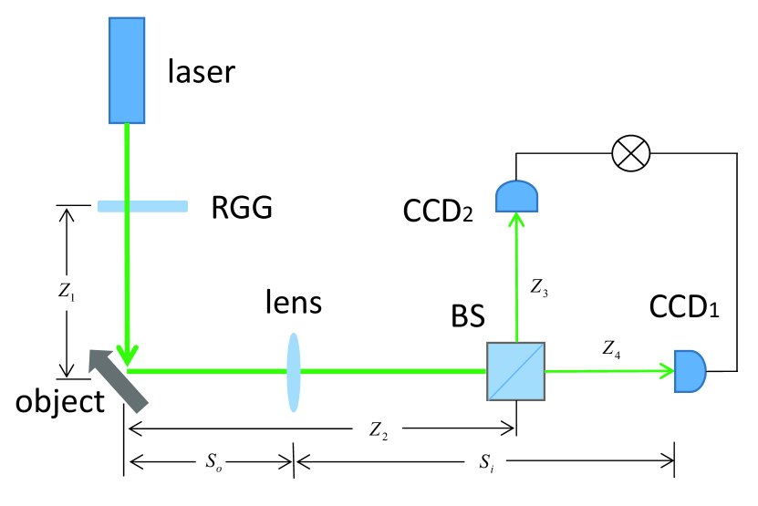
Figure 1: (Color online) The schematic of two-photon interference imaging with thermal light source. RGG: rotating ground glass, BS: beam splitter.

The reconstructed image is observed from the photon number fluctuation correlation. To calculate the photon number fluctuation correlation, we start from examining the second-order coherence function $G^{(2)}\left(\rho_{i1},\rho_{i2}\right)$, which is jointly measured by CCD1 and CCD2 on the two image planes:

$$G^{(2)}\left(\rho_{i1},\rho_{i2}\right)$$

$$=\left\langle E_{1}^{\ast}(\rho_{i1})E_{1}(\rho_{i1})E_{2}^{\ast}(\rho_{i2})E_{2}(\rho_{i2})\right\rangle$$

$$=\left\langle\sum_{m}E_{m}^{{}^{\prime}\ast}(\rho_{i1})\sum_{p}E_{p}^{{}^{\prime}}(\rho_{i1})\sum_{n}E_{n}^{{}^{\prime}\ast}(\rho_{i2})\sum_{q}E_{q}^{{}^{\prime}}(\rho_{i2})\right\rangle$$

$$=\sum_{m}\left|E_{m}^{{}^{\prime}}(\rho_{i1})\right|^{2}\sum_{n}\left|E_{n}^{{}^{\prime}}(\rho_{i2})\right|^{2}$$

$$+\sum_{m\neq n}E_{m}^{{}^{\prime}\ast}(\rho_{i1})E_{n}^{{}^{\prime}}(\rho_{i2})E_{n}^{{}^{\prime}\ast}(\rho_{i2})E_{m}^{{}^{\prime}}(\rho_{i1})$$

$$=\left\langle n(\rho_{i1})\right\rangle\left\langle n(\rho_{i2})\right\rangle+\left\langle\Delta n(\rho_{i1})\Delta n(\rho_{i2})\right\rangle.$$ (3)

The term $\left\langle n(\rho_{i1})\right\rangle\left\langle n(\rho_{i2})\right\rangle$ corresponds to the product of two identical classical images measured by CCD1 and CCD2, respectively. The interference term that generates an image in the joint photon number fluctuation measurement of CCD1 and CCD2.

$$\left\langle\Delta n(\rho_{i1})\Delta n(\rho_{i2})\right\rangle$$

$$=\sum_{m\neq n}E_{m}^{{}^{\prime}\ast}(\rho_{i1})E_{n}^{{}^{\prime}}(\rho_{i2})E_{n}^{{}^{\prime}\ast}(\rho_{i2})E_{m}^{{}^{\prime}}(\rho_{i1})$$

$$=\left|\sum_{m}E_{m}^{{}^{\prime}\ast}(\rho_{i1})E_{m}^{{}^{\prime}}(\rho_{i2})\right|^{2}$$

$$\equiv\left|G_{12}^{(1)}\left(\rho_{i1},\rho_{i2}\right)\right|^{2},$$ (4)

where

$$G_{12}^{(1)}\left(\rho_{i1},\rho_{i2}\right)$$

$$=\sum_{m}E_{m}^{\ast}\int d\rho_{o}g_{m}^{\ast}\left(\rho_{o}\right)\int dkO^{\ast}\left(\rho_{o}\right)g_{m}^{\ast}\left(k,\rho_{i1}\right)$$

$$\times\sum_{m}E_{m}\int d\rho_{o^{{}^{\prime}}}g_{m}\left(\rho_{o^{{}^{\prime}}}\right)\int dk^{{}^{\prime}}O\left(\rho_{o^{{}^{\prime}}}\right)g_{m}\left(k^{{}^{\prime}},\rho_{i2}\right)$$

$$=\sum_{m}E_{m}^{\ast}\int d\rho_{o}d\rho_{o^{{}^{\prime}}}g_{m}^{\ast}\left(\rho_{o}\right)E_{m}g_{m}\left(\rho_{o^{{}^{\prime}}}\right)$$

$$\times\int dkO^{\ast}\left(\rho_{o}\right)e^{ik\rho_{o}}somb\left(\frac{\pi}{\lambda}\frac{D}{s_{o}}\left|\rho_{o}+\frac{\rho_{i1}}{\mu}\right|\right)$$

$$\times\int dk^{{}^{\prime}}O\left(\rho_{o^{{}^{\prime}}}\right)e^{-ik^{{}^{\prime}}\rho_{o^{{}^{\prime}}}}somb\left(\frac{\pi}{\lambda}\frac{D}{s_{o}}\left|\rho_{o^{{}^{\prime}}}+\frac{\rho_{i2}}{\mu}\right|\right)$$ (5)

is the first-order coherence function. $k$ and $\lambda$ represent wave vector and wavelength respectively. $D$ is the diameter of the imaging lens. $\mu=s_{i}/s_{o}$ is the magnification factor. $s_{o}$ is the distance between the object and the imaging lens, $s_{i}$ is the distance between the imaging lens and the image plane. $\left\langle T(\rho_{o})T^{\ast}(\rho_{o})\right\rangle=\lambda O(\rho_{o})\delta\left(\rho_{o}-\rho_{o}^{{}^{\prime}}\right)$. For a perfect imaging system, the $somb$ function (or point-spread function) in the convolution of Eq.5 will be replaced by $\delta$ function. However, limited by the finite size of the imaging system, we may never have a perfect point-to-point relationship.

To calculate Eq.5, we complete the summation in terms of the sub-sources by means of an integral over the entire source plane. Thus, the Eq.5 is approximated in the follow form,

$$G_{12}^{(1)}\left(\rho_{i1},\rho_{i2}\right)$$

$$\propto\int d\rho_{o}\left|O(\rho_{o})\right|^{2}somb\left(\frac{\pi}{\lambda}\frac{D}{s_{o}}\left|\rho_{o}+\frac{\rho_{i1}}{\mu}\right|\right)$$

$$\times somb\left(\frac{\pi}{\lambda}\frac{D}{s_{o}}\left|\rho_{o}+\frac{\rho_{i2}}{\mu}\right|\right).$$ (6)

Submitting Eq.6 into Eq.4, we have

$$\left\langle\Delta n(\rho_{i1})\Delta n(\rho_{i2})\right\rangle$$

$$\propto\left|\int d\rho_{o}\left|O(\rho_{o})\right|^{2}somb^{2}\left(\frac{\pi}{\lambda}\frac{D}{s_{o}}\left|\rho_{o}+\frac{\rho_{i1}}{\mu}\right|\right)\right.$$

$$\times\left.somb^{2}\left(\frac{\pi}{\lambda}\frac{D}{s_{o}}\left|\rho_{o}+\frac{\rho_{i2}}{\mu}\right|\right)\right|^{2}.$$ (7)

Equation (7) shows that the reconstructed image can be observed by measuring the term of two-photon interference. Moreover, we will obtain a perfect image when $\rho_{i1}=\rho_{i2}$.

A significant advantage of two-photon interference imaging is that it can effectively overcome the effect of harsh optical environment, e.g. atmospheric turbulence. Next, we illustrate this feature. In order to simplify the calculation, we assume that the atmospheric turbulence is introduced between the object and the beam splitter. Thus, the light fields received by two CCD cameras can be expressed as

$$E_{1}(\rho_{i1},t) =\sum_{m}E_{m}(\rho_{m},t)g(\rho_{o})T(\rho_{o})g(\rho_{i1})e^{i\delta\varphi_{m}}$$

$$=E_{m}^{{}^{\prime\prime}}(\rho_{i1},t)e^{i\delta\varphi_{m}};$$ (8)

$$E_{2}(\rho_{i2},t) =\sum_{n}E_{n}(\rho_{n},t)g(\rho_{o})T(\rho_{o})g(\rho_{i2})e^{i\delta\varphi_{n}}$$

$$=E_{n}^{{}^{\prime\prime}}(\rho_{i2},t)e^{i\delta\varphi_{n}}.$$ (9)

The function $e^{i\delta\varphi}$ stands for the atmospheric turbulence induced phase variations. According to the above calculation process, the photon number fluctuation correlation can be expressed as

$$G^{(2)}\left(\rho_{i1},\rho_{i2}\right)$$

$$=\left\langle\sum_{m}E_{m}^{{}^{{}^{\prime\prime}}\ast}(\rho_{i1})e^{i\delta\varphi_{m}}\sum_{p}E_{p}^{{}^{{}^{\prime\prime}}}(\rho_{i1})e^{i\delta\varphi_{p}}\right.$$

$$\left.\sum_{n}E_{n}^{{}^{{}^{\prime\prime}}\ast}(\rho_{i2})e^{i\delta\varphi_{n}}\sum_{q}E_{q}^{{}^{{}^{\prime\prime}}}(\rho_{i2})e^{i\delta\varphi_{q}}\right\rangle$$ (10(a))

$$=\sum_{m}\left|E_{m}^{{}^{{}^{\prime\prime}}}(\rho_{i1})e^{i\delta\varphi_{m}}\right|^{2}\sum_{n}\left|E_{n}^{{}^{{}^{\prime\prime}}}(\rho_{i2})e^{i\delta\varphi_{n}}\right|^{2}$$

$$+\sum_{m\neq n}E_{m}^{{}^{{}^{\prime\prime}}\ast}(\rho_{i1})E_{n}^{{}^{{}^{\prime\prime}}}(\rho_{i2})E_{n}^{{}^{{}^{\prime\prime}}\ast}(\rho_{i2})E_{m}^{{}^{{}^{\prime\prime}}}(\rho_{i1})$$

$$\times e^{i\delta\varphi_{m1}}e^{i\delta\varphi_{n1}}e^{i\delta\varphi_{m2}}e^{i\delta\varphi_{n2}}$$ (10(b))

$$=\left\langle n^{{}^{\prime}}(\rho_{i1})\right\rangle\left\langle n^{{}^{\prime}}(\rho_{i2})\right\rangle+\left\langle\Delta n^{{}^{\prime}}(\rho_{i1})\Delta n^{{}^{\prime}}(\rho_{i2})\right\rangle.$$ (10(c))

The first two terms of Eq.10(c) represent the classical images output by two CCD cameras, which cannot eliminate the influence of turbulence. However, the cross interference term $\left\langle\Delta n(\rho_{i1})\Delta n(\rho_{i2})\right\rangle$ reaches its turbulence-free when $z_{3}=z_{4}$, $e^{i\delta\varphi_{m1}}e^{i\delta\varphi_{n1}}e^{i\delta\varphi_{m2}}e^{i\delta\varphi_{n2}}=1$.

III Experiments

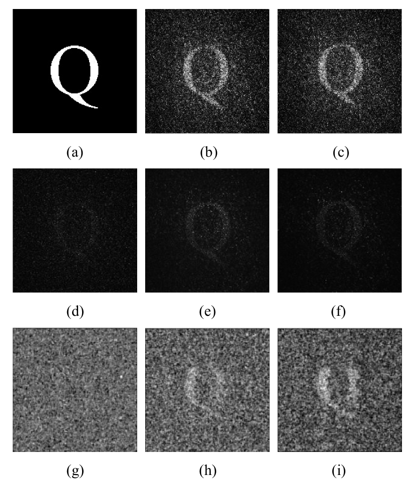
Figure 2: Top row: (a) object (letter “Q”), (b) classic image output by CCD1, (c) classic image output by CCD2 (image has been flipped). Middle row: two-photon interference image obtained by $\left\langle\Delta n(\rho_{i1})\Delta n(\rho_{i2})\right\rangle$ with different frames. The numbers of frames are (d) 10, (e) 500, (f) 1000. Bottom row: the corresponding quantum image with different frames. The numbers of frames are (g) 10, (h) 500, (i) 1000.

The experimental setup is schematically shown in Fig.1. In the setup, a standard monochromatic laser (30 mW) with wavelength $\lambda=532$nm illuminates a rotating ground glass (2$rad/$min). Thus, millions of tiny diffusers within the rotating ground glass scatter the laser beam into many independent wave packets, which generate a typical chaotic pseudothermal source with fairly large size in transverse dimension. After free propagation of $z_{1}=100$cm, the light beam illuminates the object, such as the letter “Q” as shown in Fig.2(a). The scattered and reflected photons reflected by the object is separated into two beams by a 50:50 beam splitter after propagation of $z_{2}\simeq 103$cm. one of the beam is collected by CCD1 (the imaging source, DFK 23U618) and the other is collected by CCD2 (the imaging source, DFK 23U618). An imaging lens focuses the scattered and reflected light from the object onto the two image planes (CCD plane) defined by the Gaussian thin lens equation $1/s_{o}+1/s_{i}=1/f$, where $s_{o}=60$ and $s_{i}\simeq 43$ represent object distance and image distance, respectively. $f=25$cm is the focal length of the imaging lens.

Two CCD cameras are controlled by software to collect data at the same time. A photon number fluctuation correlation circuit [25-27] is used to measure the photon number fluctuation correlation. Figure 2 reports a set of typical experimental results. Figure 2(b) and Figure 2(c) are two classic images output by the two CCD cameras in two-photon interference experiment setup, i.e., $\left\langle n(\rho_{i1})\right\rangle\left\langle n(\rho_{i2})\right\rangle$. Figure 2(d-f) is a measurement of the cross interference term $\left\langle\Delta n\left(\rho_{i1}\right)\Delta n\left(\rho_{i2}\right)\right\rangle$. It is this cross interference term that generates an image in the joint photon number fluctuation measurements of CCD1and CCD2. Figure 2(g-i) is the experimental results of conventional quantum imaging (ghost imaging). In the setup of quantum imaging, all the devices and parameters are the same as the two-photon interference imaging experiment. From Fig.2 we obtain the following conclusion: (i) The imaging quality of two-photon interference imaging is much higher than that of quantum imaging, especially when the number of samples is very small. Two photon interference imaging can produce a clear image by ten samples, which is impossible for conventional quantum imaging. The reason is that two-photon interference imaging measures the spatial resolution of both optical paths, while conventional quantum imaging only measures the spatial resolution of one optical path, the other optical path is measured by point measurement. The imaging quality of two-photon interference imaging is slightly lower than classical imaging. (ii) The imaging speed of two-photon interference imaging is much faster than that of quantum imaging and can be compared with that of classical optical imaging.

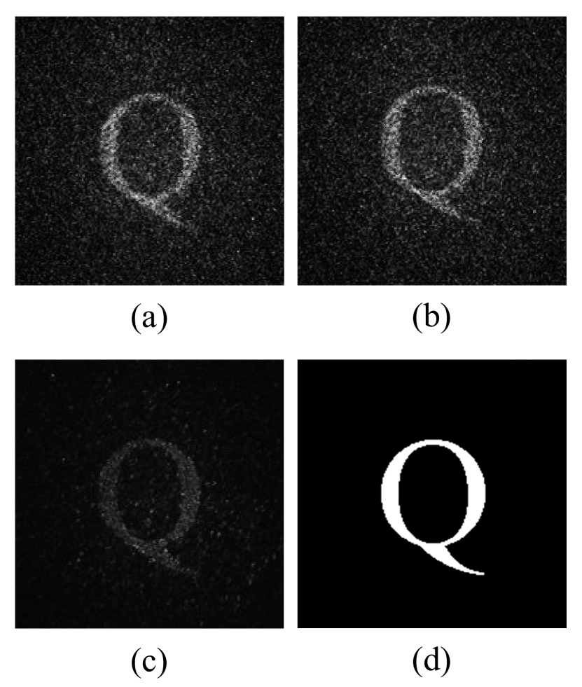
Figure 3: (a,b)Two classical images of the letter “Q” showing the distortion caused by turbulence. The shape and position of the image are changed by turbulence, which results in image distortion. (c)Experimentally generated turbulence-free two-photon interference images of a letter “Q” object using 200 frames of data measured through laboratory turbulence. (d) Object.

Next, we demonstrate the turbulence-free feature of two-photon interference imaging. In this experiment, atmospheric turbulence is introduced to the optical paths between the object and lens by adding heating elements underneath the optical paths operating at a temperature of 550${}^{\circ}{\rm C}$ with the refractive index structure parameter $C_{n}^{2}$ in the range of $1.5\times 10^{-10}$ to $1.0\times 10^{-9}$ [13]. The length of the heating area is $20$ cm. These values correspond to extremely high levels of atmospheric turbulence causing significant temporal and spatial fluctuations of light intensity. In the measurement, the two-photon interference image and classical image of the object were captured and monitored simultaneously when the turbulence was introduced to optical paths. The observations are reported in Fig.3. The experimental results show that two-photon interference imaging can effectively overcome the influence of atmospheric turbulence.

IV Conclusion

In summary, the two-photon interference imaging based on thermal light source has been demonstrated in this article. Theoretical and experimental results show that the imaging quality and imaging speed of the two-photon interference imaging is much better than that of conventional quantum imaging, and comparable to classic optical imaging. The reason is that both optical paths carry the information of the object and are measured with spatial resolution. More important, Two photon interference imaging can effectively overcome the effect of harsh optical environment. Further more, two photon interference imaging has other advantages, for example, its optical structure is similar to classical optical camera, which makes it suitable for practical application.

V Acknowledgement

This project was supported by the National Natural Science Foundation (China) under Grant Nos. 11704221, 11574178 and 61675115, Taishan Scholar Project of Shandong Province (China) under Grant No. tsqn201812059.

References

- (1) T. Young, A Course of Lectures on Natural Philosophy and the Mechanical Arts (Printed for J. Johnson by W. Savage, London, 1807).
- (2) P. R. Saulson, Fundamentals of Interferometric Gravitational Wave Detectors (World Scientific, Singapore, 1994).
- (3) P. A. Dirac, The principle of quantum mechanics (Oxford University Press, 1982).
- (4) C. K. Hong, Z. Y. Ou, and L. Mandel, Phys. Rev. Lett. 59, 2044 (1987).
- (5) L. Mandel, Rev. Mod. Phys. 71, S274 (1999).
- (6) W. H. Tan, Nonlinear and quantum optics (Science Press, Beijing, 2018).
- (7) C. Liu, J. F. Chen, S. C. Zhang, S. Y. Zhou, Y. Kim, M. M. T. Loy, G. K. L. Wong, S. W. Du, Phys. Rev. A 85, 021803(R) (2012).
- (8) T. Chaneliere, D. N. Matsukevich, S. D. Jenkins, S.-Y. Lan, R. Zhao, T. A. B. Kennedy, and A. Kuzmich, Phys. Rev. Lett. 98, 113602 (2007).
- (9) G. Scarcelli, A. Valencia, and Y. H. Shih, Europhys. Lett. 68, 618 (2004).
- (10) T. B. Pittman, Y. H. Shih, D. V. Strekalov, and A. V. Sergienko, Phys. Rev. A 52, R3429 (1995).
- (11) D. N. Klyshko, Photons and Nonlinear Optics (Gordon and Breach Science Publishers, Amsterdam, 1988).
- (12) R. E. Meyers , K. S. Deacon , and y. h. Shih, Appl. Phys. Lett. 98, 111115 (2011).
- (13) R. E. Meyers , K. S. Deacon , and y. h. Shih, Appl. Phys. Lett. 100, 131114 (2012).
- (14) W. Li , Z. Tong . K. Xiao , Z. Liu , Q. Gao , J. Sun , S. Liu , S. Han , Z. Wang , Optica 6(12), 1515-1523 (2019).
- (15) B. I. Erkmen, J. Opt. Soc. Am A 29, 782-789 (2012).
- (16) C. Q. Zhao , W. L. Gong , M. L. Chen , E. R. Li , H. Wang , W. D. Xu, S. S. Han , Appl. Phys. Lett. 101, 141123 (2012).
- (17) W. L. Gong , C. Q. Zhao , H. Yu , M. L. Chen , W. D. Xu , S. S. Han, Sci. Rep. 6, 26133 (2016).
- (18) X. Qiu, D. Zhang , W. Zhang , and L. Chen, Phys. Rev. Lett. 122, 123901 (2019).
- (19) P. Ryczkowski , M. Barbier , A. T. Friberg , J. M. Dudley, and G. Genty, Nature. Photon. 10, 167-170 (2016).
- (20) R. I. Khakimov , B. M. Henson , D. K. Shin , S. S. Hodgman , R. G. Dall , K. G. H. Baldwin, and A. G. Truscott, Nature 540, 100-103 (2016).
- (21) D. Pelliccia, A. Rack, M. Scheel, V. Cantelli, and D. M. Paganin, Phys. Rev. Lett. 117, 113902 (2016).
- (22) H. Yu, R. Lu, S. Han, H. Xie, G. Du, T. Xiao, and D. Zhu, Phys. Rev. Lett. 117, 113901 (2016).
- (23) A. Zhang , Y. He, L. Wu, L. Chen, and B,Wang, Optica 5, 374-377 (2018).
- (24) W. Martienssen and E. Spiller, Am. J. Phys. 32, 919 (1964).
- (25) H. Chen, T. Peng, and Y. H. Shih, Phys. Rev. A 88, 023808 (2013).
- (26) T. A. Smith and Y. H. Shih, Phys. Rev. Lett. 120, 063606 (2018).
- (27) Y. H. Shih, Technologies 4(4), 39 (2016).