Qd-tree: Learning Data Layouts for Big Data Analytics
Abstract.
Corporations today collect data at an unprecedented and accelerating scale, making the need to run queries on large datasets increasingly important. Technologies such as columnar block-based data organization and compression have become standard practice in most commercial database systems. However, the problem of best assigning records to data blocks on storage is still open. For example, today’s systems usually partition data by arrival time into row groups, or range/hash partition the data based on selected fields. For a given workload, however, such techniques are unable to optimize for the important metric of the number of blocks accessed by a query. This metric directly relates to the I/O cost, and therefore performance, of most analytical queries. Further, they are unable to exploit additional available storage to drive this metric down further.
In this paper, we propose a new framework called a query-data routing tree, or qd-tree, to address this problem, and propose two algorithms for their construction based on greedy and deep reinforcement learning techniques. Experiments over benchmark and real workloads show that a qd-tree can provide physical speedups of more than an order of magnitude compared to current blocking schemes, and can reach within of the lower bound for data skipping based on selectivity, while providing complete semantic descriptions of created blocks.
1. Introduction
The last decade has seen a huge surge in the volume of data collected for big data analytics. This trend has in turn driven up interest in building high-performance analytics systems that can answer queries over terabytes of data in seconds.
The first generation of analytics systems heavily leveraged fine-grained indexes such as B-Trees to accelerate query processing. However, more recently, the trend has shifted to using scan-oriented data processing strategies that exploit the high sequential bandwidth of modern storage devices. In an effort to reduce the amount of data read from disk, today’s analytics systems typically split up the data into chunks or data blocks in main memory or secondary storage. Further, they build an in-memory min-max index that stores the minimum and maximum values per block, per field, and use it to only retrieve blocks relevant to a query. A retrieved block is fully scanned, and other blocks are entirely skipped.
While tremendous progress has been made in organizing the data carefully within each block, with techniques such as columnar organization and compression, the problem of best assigning records to data blocks is relatively less explored. For example, today’s production systems usually partition data by arrival time into blocks called row groups, or use hash or range partitioning of data based on selected fields. Such techniques are unable to optimize for the important metric of number of blocks accessed (or rows touched, in case of variable sized blocks) by a given query workload. This metric directly relates to the I/O cost, and therefore performance, of the workload.
We desire blocks with two properties: (1) a semantic description, a precise description of its contents as a predicate over table fields; and (2) completeness, a guarantee that a block contains all tuples matching the given description. These properties are desirable for accelerating block retrieval and for using blocks as a local cache or partial view over remote data. Further, they allow us to consider advanced data layouts where a row is stored in more than one block, thereby exploiting additional storage budget (Sec. 6). Such data redundancy can significantly reduce the number of blocks accessed by a query, but only if we have the completeness property for blocks. Without the completeness guarantee, all blocks overlapping with a query would need to be scanned, even if a single block contains all the tuples needed for that query. Recent research on row-grouping (Sun et al., 2014) proposes the use of data mining and clustering techniques to create data blocks; the blocks have semantic descriptions based on a feature bitmap vector, but the resulting blocks lack completeness (Sec. 2 has more details).
1.1. Our Solution
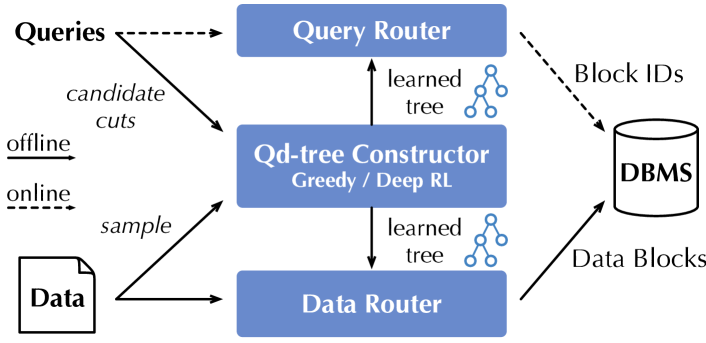
In this paper, we propose a new framework to address the problem of data organization and query routing (Sec. 2 and 3). Fig. 1 depicts our overall system architecture, targeting a traditional data warehouse scenario where data is stored on disk. At the heart of the system is a data structure we call a query-data routing tree (or qd-tree). Briefly, a qd-tree is a binary tree where each node corresponds to some sub-space of the entire high-dimensional data space. The root of the tree corresponds to the entire data space. We perform a cut of a node’s data space in order to create its children.
We can use a qd-tree for both block generation and query processing. Given a qd-tree and a dataset, we can route each tuple in the dataset through the qd-tree to assign them to data blocks of a minimum size (large blocks may be physically stored as multiple segments on storage). In other words, the leaves of the qd-tree correspond to data blocks. Each leaf has a semantic description, a predicate based on a conjunction of the cuts made to the data space as we traverse the routing tree from root to leaf. Data blocks created in this manner are also complete: a data block can be described as “all tuples that match predicate ”. Further, given a set of qd-tree based blocks and an incoming query, we can use the qd-tree in conjunction with traditional min-max indexes to quickly locate and scan all blocks relevant to the query.
Constructing the optimal qd-tree for a given dataset and workload is a hard problem. Our first approach (Sec. 4) uses a new greedy heuristic where, starting from the root, each cut is made based on locally available information. This provides routing trees of high quality with new approximation guarantees, but is unable to fully exploit long-term knowledge of tree quality. At the other extreme is dynamic programming (DP) or memoized search, which can find the optimal solution, but is infeasible given our large search space. Instead, by exploiting deep reinforcement learning (RL) for their construction, we show (Sec. 5) that we can explore a larger search space and exploit any implicit lower dimensionality of data during qd-tree construction, thereby producing routing trees that significantly outperform the state-of-the-art, while still providing complete semantic descriptions for blocks. Our RL solution can be regarded as an approximate and accelerated memoized search method (Powell, 2007, 2016), leading to higher efficiency than DP but with optimality close to DP. Deep RL-based qd-tree also forms a general framework: we show in Sec. 6 that it can easily be extended with newer types of cuts, data overlap, and data replication for even better block skipping.
We perform a detailed evaluation (Sec. 7) on a standard benchmark workload (TPC-H) and two real workloads. Our experiments show that qd-tree-based data layouts can yield physical speedups, compared to current block construction schemes, of up to per workload (or up to per query), and reach within of the lower bound for data skipping based on selectivity (the optimal solution, being a hard problem, is unknown). We cover related work in Sec. 8 and conclude the paper in Sec. 9.
1.2. Contributions
To summarize, we make the following contributions:
-
•
We introduce the qd-tree data structure and show how it can be used for data partitioning.
-
•
We propose a greedy construction scheme for qd-tree, which builds the tree top-down starting from the root, and offers theoretical approximation guarantees.
-
•
To overcome the limitations of the greedy approach, we introduce Woodblock, a deep reinforcement learning algorithm that learns to construct high-quality qd-trees.
-
•
We discuss the generality of our tree and learning framework via potential extensions that are enabled by a qd-tree’s semantic description and completeness properties.
-
•
Through a detailed evaluation on benchmarks and real workloads, we show that a learned qd-tree exhibits excellent data skipping properties.
Finally, note that one can view a qd-tree as a powerful workload-guided index for modern block-based big data analytics. It can express non-trivial block assignment strategies and can locate relevant blocks quickly during query processing. The layout within each block is orthogonal to the qd-tree itself, affecting only its cost function. For instance, a qd-tree can support columnar scan-optimized layouts as well as row-oriented layouts (possibly indexed) in each block.
2. Preliminaries
2.1. Problem Definition
Given a set of tuples , we aim to partition them into multiple blocks, such that the number of tuples required to scan for a workload is minimized, or equivalently, the number of tuples that can be skipped for the workload is maximized. Consider a partitioning over , i.e., is a set of disjoint subsets of whose union is . Each subset is called a block. We use to denote the number of tuples that can be skipped when we execute all the queries in a workload . For a scan-oriented system, it can be calculated as:
| (1) |
where is a binary function indicating whether partition can be skipped when processing query . The definition of depends on the type of meta information maintained at each block. The most common type of meta information is the max-min filters, i.e., the maximal and minimal values of each dimension over all the tuples in a block. For this case, if the hypercube defined by the max-min filters intersects with the range of query .
Given a workload , the overall effectiveness of a partitioning is measured by the total number of tuples skipped . Without constraints on block size, the number can be trivially maximized by putting every tuple in an individual block. For reasons like I/O batching and columnar compression, a real system requires blocks to have certain minimal size, e.g., 1 million tuples in SQL Server (Larson et al., 2013). We use to refer to this minimal size.
The partitioning problem is formulated as follows.
Problem 1 (MaxSkip Partitioning).
Given a set of tuples, a workload of queries, a skipping function , and a minimal block size , find a partitioning to maximize , s.t. for all .
This formulation is appropriate for static data. To handle dynamically ingested data, it is desirable to learn a partitioning function from offline data, and apply the function to online data ingestion to save data reshuffling cost.
Problem 2 (Learned MaxSkip Partitioning).
Given a set of tuples, a workload of queries, a skipping function , and a minimal block size , find a partitioning function , such that for the next tuples ingested, the partitioning generated by maximizes .
In general, no partitioning function is guaranteed to work for future unseen data. In this work, we focus on the scenario where the current tuples have the same distribution as the next tuples. Therefore, solving Problem 2 is reduced to solving Problem 1 in addition with a descriptive partitioning function, such that any new tuple can be mapped to a right partition identifier. For efficiently ingesting data, we also desire the partitioning function to be lightweight to compute.
2.2. Current Approaches
2.2.1. Date Partitioning
In this basic partitioning scheme, we partition data by time of ingestion. The skipping function if query ’s date range intersects with partition , and is otherwise.
2.2.2. Bottom-up Row Grouping
This technique was proposed by Sun et al. (Sun et al., 2014), and uses feature-based data skipping. Basically, each feature is a predicate over the data. features are extracted from the workload in the beginning using frequent pattern mining. Each block has a bitmap of length , indicating whether predicate is satisfied by any tuple in this block. If the -th bit for this block is 0, i.e., no tuple satisfies , then we can skip all queries subsumed by (i.e., stricter than) . Sun et al.’s problem formulation is slightly different, requiring each partition to have equal size. They name the problem Balanced MaxSkip Partitioning, and prove its NP-hardness by reduction from hypergraph bisection. Using the same reduction technique, we can prove that Problem 1 is NP-hard.
Sun et al.’s solution uses bottom-up clustering and is actually a solution to Problem 1, rather than the Balanced MaxSkip Partitioning problem. This is because the output of that algorithm has varying block sizes, and the sizes are no smaller than . The algorithm converts tuples into unique binary feature vectors, and record the weight of each unique feature vector (row weight), as well as the number of queries subsumed by each feature (column weight). Initially every unique feature vector is in its own block. Then blocks are merged greedily using a heuristic criterion: in each iteration, a heuristic penalty is calculated for all pairs of blocks; and the pair with lowest penalty is chosen to be merged into a new block. Once the size of a block reaches , it does not further merge with other blocks. Hence, merging eventually stops with every block having size no smaller than .
This solution is shown to be more effective than date partitioning and simple multi-dimensional range partitioning. There are several drawbacks of that approach. First, the heuristic penalty criterion used in the greedy algorithm only matches the optimization objective when the query sets subsumed by all features are disjoint. In general that assumption is not true. So choosing the pair of blocks minimizing the penalty does not necessarily maximize . Second, no theoretical guarantee is provided by the greedy merging algorithm. Third, the complexity of the algorithm is quadratic to the number of unique feature vectors, which can be as large as the number of tuples and grows exponentially with respect to the number of features. Practical application of this algorithm requires using a small number of features, which poses an additional challenge of selecting a good, small set of features. Last, while each block can be described using the “OR” of all the feature bitmap vectors contained in that block, such description is not complete. For example, there can be two blocks with identical bitmap description, and a new tuple does not have a deterministic destination partition using this description.
3. Qd-tree
A qd-tree describes how a high-dimensional data space is cut. Each node corresponds to a subspace of an -dimensional table, modeled as a discrete hypercube, . Each node logically holds all records that belong to its hypercube. The root of the tree, , represents the whole table. We assume that the domain of each dimension is known, and its attribute values are in .
Each internal node has two children, where the left child satisfies a particular predicate —attached to node —and the right child satisfies . For now, we assume each predicate to be a simple unary form, (attr, op, literal), where op is a numeric comparison, but the framework supports arbitrary predicates as well. We call predicate a cut on node .
qd-tree differs from the classical k-d tree (Bentley, 1975). k-d tree can be seen as a simple form of qd-tree, in that they typically come with heuristics such as assuming cuts to be unary, cuts alternating among dimensions, and cuts points chosen as each dimension’s median value. qd-tree does not assume these construction heuristics.
Example. Figure 2 shows an example qd-tree on two columns, (cpu,mem). The root is cut with predicate . The resultant two children are cut with and , respectively. In our implementation, the literals, e.g., “”, are dictionary-encoded as integers.
We next describe the usage of qd-tree in data routing and query processing. We later present algorithms to construct qd-tree in Sections 4 and 5.
3.1. Routing Data
Our overall strategy is to use a qd-tree to assign data to blocks on storage. The routing of data to blocks is carried out as follows. Each record “arrives” at the root and is recursively routed down. At each node, the tagged predicate is evaluated; if is true, it is routed to the left, otherwise to the right. Each record uniquely lands in a leaf due to the binary split ( or ). Each leaf thus represents a set of physical blocks to be persisted. Records are stored with an additional block ID (BID) field to denote the block they belong to, and the dataset is partitioned by this field.
In practice, we route large batches of records at a time, taking advantage of vectorized instructions. Further, threads can load different batches of records in parallel (assuming the appends at the leaves are protected with locking).
3.2. Semantic Description of Nodes
| Fields of node | Definition |
|---|---|
| n.range | Hypercube describing the node’s subspace. -dimensional array. |
| n.categorical_mask | Map: categorical column ’s name -dim of bits. 0 means that value is not present. |
As mentioned above, each allowed cut (predicate) is of the form (attr, op, literal). We allow each operator to be range comparisons, , or equality comparisons, . We now describe what node metadata we need to store to process each cut. Table 1 presents a summary.
Handling range comparisons is straightforward, as we only need to restrict a parent’s hypercube description. For example, Figure 2’s root node has the hypercube
and the cut on this node, , produces two restricted versions for its left and right child,
| left.range: | |||
| right.range: |
Handling equality comparisons, i.e., and IN, requires storing additional metadata. We assume that these predicates are only issued to categorical columns. Each node stores, for each categorical column , a -dimensional bit vector, representing the distinct values of this column. If 1 is present at a position, the value that corresponds to that position may appear under the node’s subspace; otherwise, if 0, that value definitively does not appear. It is then straightforward to process and IN cuts, by simply keeping (for the left child, since it satisfies the cut) or zeroing out (for the right child) the corresponding slots in the bit vector. For example, consider a categorical column, . The root is initialized with
since any of the three values may potentially appear. If we cut the root with (say, second value in the ordered domain), the left and right child would have the following categorical masks:
| left.categorical_mask: | |||
| right.categorical_mask: |
because the right child must satisfy . Overall, this scheme is similar to “dictionary filtering” in popular persistent formats such as Parquet.
Thus, make up a node’s semantic description. We make an optimization in the case of when data has fully been routed down a qd-tree. In this scenario, we can freeze the tree and replace each leaf’s range with a min-max index over the leaf’s records. The min-max index serves to “tighten” the range hypercube.
Each node of the qd-tree has a semantic description as described. Further, based on our routing strategy, the blocks assigned to each leaf together have the completeness property, i.e., for a given leaf’s semantic description, every record satisfying the description is stored at the corresponding leaf.
3.3. Query Processing
A simple way to process queries is to directly execute them on a dataset partitioned by the block ID (BID) field introduced by qd-tree (Sec. 3.1). In this case, which requires no intervention during query processing, the traditional partition-pruning (Moerkotte, 1998; Graefe, 2009; Dageville et al., 2016) block-level indexes (e.g., min-max) are used for actual block-skipping on a best-effort basis. For further effectiveness, we instead intercept queries submitted by users and augment them to effectively use qd-tree for partition pruning as follows. Queries are routed through the qd-tree and augmented with a BID IN (…) clause that lists the pruned set of block IDs. Modern databases can use this explicit predicate to prune blocks, without modifications to the database internals. If desired, the query routing functionality can also be integrated into the DBMS to make the process entirely transparent.
To obtain the BID list, we loop over each leaf description, check whether the query logically intersects with the leaf subspace, and return the IDs of all intersecting leaves. Concretely, for any (unary) range predicate (recall from last section, these include ), we perform a simple interval intersection check against each leaf.range. For any equality predicate ( and IN), we check the corresponding bit vector slot in leaf.categorical_mask. Alternatively, we could also “route” the query down the tree to reach a set of leaves; however, we find scanning leaf metadata to be efficient enough, especially when leaf metadata is grouped together for fast access.
Building on top of checks for predicates, the intersection checks for queries are natural extensions. We allow a query to be arbitrary conjunction or disjunction of unary predicates (and of lower-level conjuncts/disjuncts). The intersection logic for AND is simply that it intersects if all of its conjuncts do. Likewise, an OR intersects if any of its disjuncts does.
3.4. Choosing Candidate Cuts
Prior to discussing algorithms to construct qd-tree, we describe choosing the set of allowed cuts. This set serves as the search space for the construction algorithms.
We opt for a simple treatment. Since we are given a target workload of queries, we simply parse them through a standard SQL planner and take all pushed-down unary predicates as allowed cuts. For example, from a target query:
SELECT ... FROM R
WHERE (R.a < 10 OR R.b > 90) AND (R.c IN (0,4))
three cuts are extracted: (1) R.a < 10, (2) R.b > 90, and (3) R.c IN (0,4). We find that our algorithms can easily handle a few hundreds to low thousands of candidate cuts.
4. Greedy Construction of qd-tree
The construction of a qd-tree is an NP-hard combinatorial optimization problem. Greedy algorithms are a typical family of solutions that are usually efficient and make locally optimal choices. Hence, we start by proposing a greedy algorithm to construct the qd-tree. We begin with all the tuples in a single block, i.e., the qd-tree has a single root node that contains all the tuples. In each iteration, we split a leaf node whose size is larger than into two child nodes, and make sure the two children have size at least . When choosing the cut for a node, we use the one that maximizes , i.e., the number of tuples skipped by the partitioning induced by qd-tree . The idea is similar to decision tree construction, except that in decision tree learning, the predicate is chosen using a different criterion such as information gain.
To present the algorithm, we define an action as applying cut to node in a qd-tree . The result of action is denoted as . In , node becomes the parent of two child nodes: the left child contains all the tuples in satisfying , and the right child contains all the tuples in satisfying .
Our algorithm is presented in Algorithm 1. The main computation is to choose the cut that maximizes the greedy criterion for each node . For each level of the tree, the cost to executed the for loop is bounded by . The total cost of the while loop is bounded by , where is the final depth of the tree. . In the worst case, when the tree is least balanced, the complexity is quadratic to . In the balanced case, the complexity grows as . If the number of partitions is a constant, then the cost is linear to .
Approximation Guarantee
Under certain generic assumptions, we can prove that the greedy algorithm has a multiplicative offline approximation guarantee, and an additive online approximation guarantee. To the best of our knowledge, this the first algorithm with such guarantees. Our proof technique defines a new notion of submodularity: tree submodularity. We are unaware of notions of similar kind in other tree construction algorithms.
Let be the number of leaf nodes in a qd-tree. The total number of nodes is . While the result of the greedy algorithm is invariant to the order of leaf splitting (which leaf to split at each iteration), we fix the order to be top-down, left-to-right for ease of analysis. In each iteration , a cut is chosen for the leftmost node on level . We define this action as . To characterize the properties of , it is useful to define an encoding of the qd-tree.
Definition 0 (Action Encoding).
An action encoding of a qd-tree is the sequence of cuts chosen following the top-down, left-to-right order. We denote the tree after iteration as , and .
After applying action , a leaf node is split into two child nodes. By definition, .
Definition 0 (Tree Submodularity).
Given two nodes and in qd-tree , and actions . If is an ancestor of , let be minus all descendants of . We say a qd-tree space is tree-submodular if for any such in the space, .
This property means that applying a cut in qd-tree has a diminishing return as the tree grows deeper. Let be the set of queries that can be skipped by . We have the following sufficient condition for the qd-tree space to be tree-submodular.
Lemma 3.
The qd-tree space is tree-submodular if the conjunction of cuts and cannot skip any query besides for all candidate cuts and .
For example, if the workload only consists of conjunctive range queries, and each cut is a range predicate, the above condition is satisfied.
Theorem 4.
If the qd-tree space is tree-submodular, the greedy top-down construction algorithm produces a qd-tree whose overall skipping capacity is no worse than:
(a)
(b)
where refers to the skipping capacity of the optimal qd-tree , and refers to the sub qd-tree in by removing all the leaf nodes.
Bound (a) is an online bound because it depends on the algorithm output and . Bound (b) is an offline bound independent of the algorithm output. For space reasons, we defer the proofs to our technical report (Yang et al., 2020).
5. Qd-tree using Deep RL
The greedy technique presented above makes locally optimal choices which may lead to global suboptimality. At the other extreme is dynamic programming (DP), or equivalently, memoized search. It can find the optimal solution, but is infeasible given our large high-dimensional search space, leading to a need for approximate DP (Powell, 2007, 2016). In this paper, we propose leveraging deep RL to perform an approximate, accelerated, and incremental memoized search.
Woodblock is our deep RL agent that constructs routing trees optimized for a target dataset and workload. At a high level, the algorithm repeatedly constructs many trees, initially making random cuts (i.e., randomly sampling a tree from the set of all valid trees), and gradually learns to identify better cuts through rewards. After attempting a fixed number of trees or if a timeout is reached, the best tree found is deployed. This approach brings several key benefits:
-
•
Instead of remembering all the exact search states and the optimality (reward) for them, it featurizes the states and uses a model to predict the reward under the states.
-
•
Instead of enumerating all the follow-up actions of a search state to observe the reward from each of them, it samples a subset of such actions and updates the model from the observed rewards.
-
•
It can incrementally produce better trees, letting us deploy solutions quickly based on time or CPU budgets.
We next start with motivating arguments to illustrate the above intuition, and then present Woodblock in detail.
5.1. Motivation for RL
Routing tree construction presents several unique challenges that we argue are good fit for RL.
First, the exact goodness of a tree is only measurable after the whole tree is completed. Typically, a tree is completed after dozens or hundreds of cuts. Thus, when deciding what cut to make, we either approximate its benefit at that single step (e.g., a greedy criterion), or we randomly sample a cut from some (learned, gradually refined) distribution, and then accurately attribute benefits of each decision once the true goodness is calculated. We will show long-term consideration leads to higher quality trees than greedy consideration. RL methods are thus a natural fit because they study the optimization of long-term, cumulative rewards.
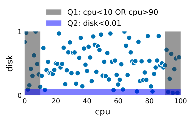
Second, an RL method does not make assumptions on the query or data distribution. It requires only a black-box learning signal, the skipping quality of a tree. To be concrete, we now present a microbenchmark to showcase the potential advantage due to this generality.
In Figure 3, we plot a simple dataset with two columns, (cpu, disk). We draw and . Query 1 is a disjunctive query on (perhaps looking for anomalies at either ends), and Query 2 is a unary filter on . Recall from last section that the optimality proofs of our Greedy construction relies on the tree-submodularity. When the query workload contains disjunctive range queries and the candidate cuts are only simple range predicates, tree submodularity is not satisfied. Our Greedy algorithm is forced to choose the cut on —since, the two cuts on provide zero skipping capability (making either cut cannot skip Q1 nor Q2), whereas the cut on provides a non-zero gain. This results in a layout of the following two blocks:
-
•
Block 1:
-
•
Block 2:
Thus, Q1 has to scan the large portion of unselected records in the middle. Our deep RL agent, Woodblock, is able to produce a better partitioning:
-
•
Block 1:
-
•
Block 2:
-
•
Block 3:
-
•
Block 4:
Hence, under this layout, both Q1 and Q2 can skip block 4, which contains a majority of records. This showcases the power of RL as a black-box optimization method.
Lastly, a large search space needs to be navigated. The number of candidate cuts can be large, potentially or . Further, the number of data dimensions can be in the dozens or hundreds. Deep RL (compared to classical RL) methods have shown successes in tackling such high-dimensional problems For instance, OpenAI Five (OpenAI, 2018), a deep RL agent for successfully playing Dota, considers an action space of dimensions and an -dimensional observation space. Our Woodblock agent uses the same scalable learning algorithm as OpenAI Five, taking advantage of recent algorithmic advances.
We next describe the detailed design of Woodblock, a deep RL agent that learns to construct qd-trees.
5.2. Woodblock: the Deep RL agent
To apply any RL algorithm, we first need to define the tree construction Markov Decision Process (MDP). The state space, , is defined to be any subspace of the entire data space of the relation under optimization. The action space, , is the set of allowed cuts. Taking an action (cut) on a state (node) produces two new states, which we append into a queue for exploration. The queue is initialized with a root state (the root node) when starting each tree construction.
The Woodblock agent, at its core, consists of two learnable networks parameterized by : (1) the policy network, , takes a state and emits a probability distribution over the action space (“given a node, how good are the cuts?”), and (2) the value network, , estimates the expected cumulative reward from a given state.
Sequentially, the agent (1) takes a node off the exploration queue, (2) evaluates its current policy, , (3) samples an action from this output distribution, (4) applies the sampled action (cut) on node to produce new nodes. We use Proximal Policy Optimization (PPO) (Schulman et al., 2017) as the underlying learning algorithm, a variation in the policy gradient family of methods. This update rule is used as a black-box subroutine and is not fundamental to the design of Woodblock.
Intuition. We start each episode (the construction of one tree) with the root state (the singleton tree with a root node). The agent takes actions and transition into next state(s). Once a stopping condition is reached, described next, the episode is ended and we obtain a completed qd-tree. We calculate the reward of this episode, i.e., the data skipping ratio achieved by the tree, and invoke PPO for gradient updates to . With the updated behaviors, the agent starts the next episode. Through repeatedly constructing qd-tree, the RL agent becomes better. At the beginning of training, a randomly initialized implies random behavior: random cuts are made and the skipping ratios would not excel. However, as more trees (episodes) are explored, the refined is encouraged to make cuts that achieve higher skipping ratios.
We next discuss algorithmic details.
5.2.1. Stopping Condition
To prevent an endless sequence of cuts, we must define an appropriate stopping condition. A naive condition would be stopping after a pre-determined number of cuts are made. This is problematic, because we do not know a priori the number of cuts required to achieve good data skipping for a given dataset-workload.
Instead, we connect back to Problem 1’s requirement where each leaf block must contain at least records. The agent is allowed to make a cut on current node , if the resultant children (approximately) contain more than records.
This approximation is achieved by testing the cut on a data sample. First, at algorithm initialization, we take a data sample of ratio from the dataset (we find to generally work well). All episodes (the exploration of trying out different trees) reuse the fixed sample. The data sample is assigned to the root node. Next, as a cut is made, we evaluate the cut on the data sample, and obtain a subset of records that satisfy it and a subset that does not. If both have more than records, we call the cut legal and allow it to proceed. Lastly, if a current node has no legal cuts in action space, we stop cutting on it and form a leaf.
5.2.2. Reward Calculation
After a tree is produced, Woodblock calculates rewards for all actions taken. The rewards serve as important learning signals: they allow the agent to learn to distinguish profitable cuts.
First, we define , the number of skipped records under node across all queries:
Recall from Equation 1 that refers to the number of records skipped across the workload. Here, n.records is the set of records routed to node during tree construction—thus a subset of the small data sample we take. Since the sample is small, this ensures reward calculation is efficient.
We then assign a reward for every action taken, i.e., for every intermediate node and corresponding cut :
Namely, we normalize number of skipped records under to by scaling with , where the denominator is the maximum number of skipped records possible under (the best case of all queries skipping all its records). The PPO update rule is then invoked with a list of state-action-reward tuples.
5.2.3. Implementation
This section discusses detailed implementation of the networks. The policy network and the value network have shared weights, which are two fully-connected layers, 512 units each, with ReLU activation. Each network has its own output layer: for the policy network, it is a -dimensional linear projection; for the value network it is a scalar projection.
Each state is featurized as the concatenation of n.range and n.categorical_mask. Due to the potentially large values in the former component, we binary-encode both vectors (i.e., these vectors are encoded in bits). The action space is a discrete categorical distribution, usually with a dimensionality in a few hundreds.
We found that neural network computation is not a bottleneck in our setup. Routing records and calculation of rewards, on the other hand, take up a significant portion of tree construction time. We therefore only use CPUs for our agent (although using a GPU for neural network computation yields a slight overall speedup).
5.2.4. Related Work
Our formulation of using deep RL to learn a tree under custom quality metrics is inspired by NeuroCuts (Liang et al., 2019), a deep RL algorithm to construct packet classification trees. We compare the two work below.
First, Woodblock adopts their overall approach of tree-structured MDP: each node is treated as an independent state, and receives a normalized reward as if the agent is asked to start constructing a tree from that node. This means the agent is tasked to solve each subproblem independently.
Second, while NeuroCuts assumes no knowledge of workload, Woodblock optimizes a target data-workload pair. This affects the choice of the actions. Their action space includes generic actions (e.g., “cut dim K in N equal parts”) while we obtain our actions from the unary predicates of the target workload. We find that such generic actions do not make sense in our setting—the domain of an attribute can be large, and cutting at non query-aligned literals is suboptimal.
Third, we make specific optimizations for our data analytics setting. A data sample is required for us to calculate invalid cuts and respect the layout constraints. We also propose special treatment of categorical predicates in featurization.
6. Framework Extensions
Having described two algorithms to construct a qd-tree, we are now in a position to discuss extensions to our framework.
6.1. Advanced Cuts
Thus far we have assumed the candidate cuts are single-column predicates (Section 3.4). They are desirable because their simplicity allows for fast evaluation during tree construction. Nevertheless, qd-tree can be extended to support binary cuts of the form (attr1, op, attr2). Recall from Table 1 there are two components of a node’s semantic description, and neither of them can describe a binary cut. We append a new component to each node ’s description:
| n.adv_cuts: a bit vector of size —AC— |
where the constant denotes the number of advanced cuts to support and is specified for each workload a priori. Each position corresponds to “does this node contain records that satisfy advanced cut ”, with zero indicating no and one indicating potentially yes. This is the same semantics as categorical_mask.
For instance, the TPC-H workload contains non-join binary filters such as:
-
•
: c_nationkey = s_nationkey
-
•
: l_shipdate < l_commitdate
-
•
: l_commitdate < l_receiptdate
A vector of thus indicates the first condition is definitely not met (i.e., it describes a subspace of records whose c_nationkey does not equate s_nationkey).
Lastly, the same mechanism also handles LIKE predicates or even stateless UDFs (with the caveat that, clearly, the cost of evaluating the predicates depends on their inherent complexities). The user can impose a limit on the maximum number of advanced cuts to support.
6.2. Data Overlap
With the abundance of cheap storage in the cloud, one desirable feature for an analytics system is to trade space for potentially faster execution time. A fruitful line of work has dedicated to this problem, e.g., materialized views, which we review in related work. We now discuss how qd-tree can also naturally support duplicating data.
Figure 4 shows a 2D synthetic dataset and four queries. Naively invoking either Greedy or Woodblock to construct a qd-tree for this dataset-workload is suboptimal. Any sequence of cuts—recall, the cut points are query literals, i.e., any of the edges in the figure—would lead to 4 blocks: one with N+1 record, and three with N records. (This is due to the binary nature of the cuts.) The three blocks would have to fetch the singleton record they need from the first block. Hence, a total of extra tuples are read.
We extend qd-tree construction to handle such data overlap cases as follows. Observe that the reason the “lucky” -record block is not further cut is due to the minimum block size constraint, . We can instead launch either of our construction algorithms with a relaxed cutting condition: allowing one of the children to have size smaller than . With this change the lucky block would be further cut into an -record one and a block with the singleton record.
Once such a qd-tree is constructed, we loop through all produced leaves, and partition them into two sets: those with size and those with size (the original constraint). We then replicate each block in the small-size set to any of its neighbor blocks in the large-size set. We define two blocks to be neighbors if their hypercubes have dimension boundaries in common and the intervals at the remaining dimension are adjacent. This ensures that, with minor modifications to node metadata, the semantic descriptions preserve completeness. With this scheme, our algorithms could reach the optimal partitioning for the scenario in Figure 4 at virtually no extra storage cost.
6.2.1. Data and Query Routing
Data routing occurs as before, with a row routed to all matching blocks. Rows landing in a replicated block are simply copied to every replica. For query processing, the candidate set of blocks to be considered includes all blocks that overlap with the query rectangle. However, we can leverage the completeness property of blocks to prune out blocks that are redundant. For example, a query that asks only for the centre rectangle (with the singleton record) in the example above does not have to fetch all blocks, even though the min-max index for all four blocks includes it. This is because of our semantic descriptions and completeness properties: we can prune away the other blocks because the first block completely covers the query rectangle. With overlap, the set of blocks scanned when evaluating a query may contain duplicate rows. To eliminate them, when scanning block ID , we can simply ignore tuples that match the semantic description of any selected block with ID . A detailed evaluation of these strategies is left as future work.
6.3. Data Replication: two-tree approach
Full-copy data replication is a complimentary approach to overlap in utilizing extra storage. The extension for qd-tree construction to support such replication is natural.
First, we learn (using Greedy or RL) a qd-tree, , optimized for the full workload . Then, we can in fact build a second qd-tree, , tailored for the queries that experience the worst skippability under tree . The second tree is a logical copy of the entire dataset. When constructing the second tree, we modify the reward function for RL (and the greedy criterion for greedy), by accounting for the existence of the first tree. For each query , we choose one of the two trees which maximizes the skippability for , and calculate the number of skipped tuples using that tree. Then we sum up the ’s for all . This change naturally guides the construction of the second tree to focus on the queries with low skippability by . Additionally, the first tree can be re-built and re-optimized with fixed, and iterate. Since the revised reward function keeps increasing and is upper bounded, this process eventually converges. The idea may also be extended to more than two trees if needed. Exploring such extensions is a rich area for future work.
7. Evaluation
We now experimentally evaluate our designs. We highlight key findings from the evaluation:
-
•
(Table 2) qd-tree-based layouts enable excellent data skipping (– over the state-of-the-art).
-
•
Greedy construction of qd-tree produces high skipping ratios; yet, Woodblock, using a general-purpose RL algorithm, can still produce up to gains due to its optimization of the long-term objective.
- •
7.1. Setup and Metrics
We implement qd-tree as a lightweight Python library. It includes a lightweight AST and associated query-processing logic. We use the vectorized arithmetics in numpy and pandas. Woodblock, the RL agent, is implemented using Ray RLlib (Liang et al., 2018; Moritz et al., 2018), a scalable reinforcement learning library. We evaluate all systems using both logical and physical metrics.
Logical: Access Percentage. We report %tuples accessed for the whole workload achieved by various partitioners. This metric is lower bounded by the true workload selectivity, and lower values indicate greater potential I/O savings.
Physical: Query Runtime. We report end-to-end execution time as queries are issued over several analytics systems:
-
•
Single-Node Spark (v2.4): All layouts execute with Spark over Parquet files stored on disk (HDD). After a qd-tree is constructed, each leaf block is converted into a Parquet file. Other baseline layouts are stored as Parquet files as well in comparable number of blocks.
-
•
Commercial DBMS: We use a commercial standalone black-box optimized DBMS. We model a scenario where partitioning (e.g., by tenant ID, query ID, or TPC-H month) is used for parallelism at a higher level, by limiting each individual query to a single degree of parallelism. We first load the datasets under different layouts into the system, which uses its own binary columnar storage format on a local SSD.
-
•
Distributed Spark: We use a 4-node Spark cluster hosted on Microsoft Azure, each with 8 vCPUs, 56GB RAM, and an SSD. All data is stored as Parquet files (as with single-node Spark) on Azure Storage, a remote blob store. The qd-tree is cached at the driver for query rewrites.
We ensure that all layouts have a comparable number of blocks. To eliminate caching effects we clear the OS buffer cache before each query run. To evaluate the benefit of qd-tree query routing, we execute queries using explicit BID filters (Section 3.3; the default), or without (called no route).
7.2. Workloads
We evaluate on (1) TPC-H and (2) two real-world workloadsfrom a large commercial software vendor.
TPC-H. We generated TPC-H with a scale factor (SF) of 1000. Following prior work (Sun et al., 2014), we denormalize the TPC-H schema for the purpose of obtaining a table that many filters touch111Our technique can layout each table in the database independently using predicates over that table. Jointly optimizing the layout of multiple tables for complex join queries is left for future work.. Due to the uniform nature of TPC-H data, we apply all partitioning techniques to an one-month partition of the dataset; the month-partition totals 77M tuples, 68 columns, and 85GB. For queries, we include all templates that touch the line_item fact table222Our goal is to find a table with a rich set of filters. To achieve this, we denormalize all tables and include all templates that touch the fact table.. This includes the same 8 templates (, , , , , , , ) that (Sun et al., 2014) uses, as well as 7 additional templates: , , , , , , . We use 10 random seeds to generate each template, resulting in a total of 150 queries. The overall scan selectivity is 21.3%.
Real Datasets. Our first real dataset, called ErrorLog-Int, consists of error logs collected from internal customers of a large software vendor. The error logs correspond to kernel crash dump reports and are collected in real-time and loaded into a data warehouse for analysis. These error logs contain information such as a categorical event type (e.g., device crash, live kernel event, etc.) with distinct values, OS build date, OS version (string), client ingest date, and entry validity (a boolean). The dataset has columns. We collect a sample of around one week of logs, amounting to million records and GB of raw data. The dataset is also associated with a query workload imposed by automated systems via an API and users through a user interface and translated into stored procedures over the data. We extract the predicates that are pushed to storage and extract a set of queries over dimensions that represent a majority of the workload. The overall workload selectivity is %; thus, individual queries return very few results on average, usually less than . All queries are of the form of IN predicates over the categorical data, along with date ranges and LIKE and equality predicates over the string fields.
Our second real dataset, called ErrorLog-Ext, is also a crash dump log, but is collected from external customers (applications) around the world. This dataset is fundamentally different from the earlier one, collected over days with million rows (GB), has more dimensions () and a much larger categorical domain of around distinct values. We also use 1000 queries, which return more results on average, with an overall scan selectivity of .
7.3. Approaches
We compare layouts produced by different algorithms, spanning from heuristics used in industry practice to the state-of-the-art approach in literature:
-
•
Random baseline (TPC-H): a partitioner that simply shuffles records into fixed-size blocks.
-
•
Range baseline (real workloads): range-partitioning on an ingest time column (the default scheme deployed for the real workloads).
- •
-
•
Greedy-constructed qd-tree (Sec. 4).
-
•
Woodblock-constructed qd-tree (Sec. 5).
We ensure Bottom-Up, Greedy, and Woodblock have the same search space: the same set of candidate cuts is fed to the latter two approach, which is also fed to Bottom-Up as input to their feature selection procedure. The feature selection procedure first performs a topological sort of the features according to the subsumption relationship, and then select features one by one. The frequency of each feature is initialized as the number of queries subsumed by that feature. At each iteration, a feature not subsumed by any others is chosen, and the frequency of all the other features is discounted if the they subsume common queries with the chosen feature. A feature will not be chosen if its frequency is below a threshold. We configure Bottom-Up to use up to 15 features, which follows the number reported in (Sun et al., 2014). We set , the minimum number of records per block, to K for TPC-H and K for the two ErrorLog workloads.
7.4. TPC-H
| Workload | Baseline | Bottom-Up | Greedy (ours) | RL (ours) |
|---|---|---|---|---|
| TPC-H | 56% | 46.1% | 26.3% | 25.8% |
| ErrLog-Int | 100% | 3.1% | 0.4% | |
| ErrLog-Ext | 100% | 0.2% |
Table 2 shows the percentage of tuples accessed for different layouts on the TPC-H workload. Overall, qd-tree layouts provide up to 1.8 savings compared to Bottom-Up.
7.4.1. Physical execution
We report the execution runtime of TPC-H on (1) a distributed Spark cluster, and (2) a single-node commercial DBMS.
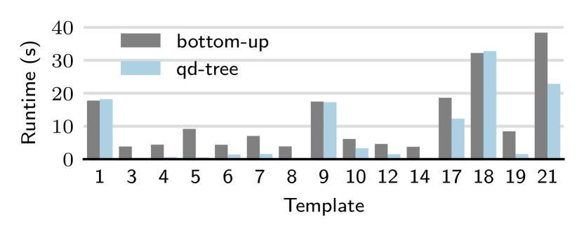
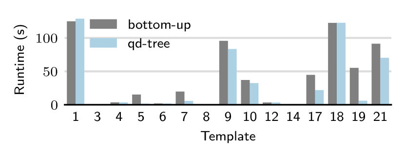
Distributed Spark. Figure 5(a) shows the mean runtime per template on distributed Spark (each template has 10 random instances). In total, qd-tree yields a speedup of (closely matching the logical ratio in Table 2). When excluded templates that need to scan all data, the speedup is .
The top three templates where qd-tree exhibits the most absolute runtime reduction are . For , the advanced cut l_commitdate ¡ l_receiptdate allows many blocks to be skipped, substantially speeding up a self-join. has filters on supplier’s r_name, a categorical with diverse literals—qd-tree yields a speedup on this template. is an OR of three complex 6-filter blocks; qd-tree is able to optimize for this complex template and provides speedup over Bottom-Up. Bottom-Up is faster only on and , both of which require the full month worth of data.
Commercial DBMS. We move to a second execution engine, the commercial DBMS, to investigate whether qd-tree still provides physical runtime execution. Results are shown in Figure 5(b). Over all templates, qd-tree has a speedup of and when excluding the scan-all templates, the speedup is . Consistent with SparkSQL results, templates exhibit large speedups of respectively. Relative ratios for other templates are also consistent, which suggests that the benefits from improved layouts carry over.
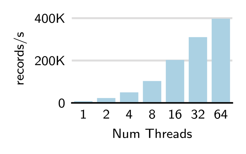
Performance of data and query routing. Figure 6(a) reports the throughput of routing records through a qd-tree (i.e., ingestion). We vary the number of ingestion threads on the same machine; linear scalability is achieved with up to 16 threads, and at 64 threads, our prototype implementation in Python (which uses vectorized operations when possible) can reach 400K records/second. Higher throughput can be reached still, by either an optimized implementation in a compiled language, or by scaling out to multiple nodes.
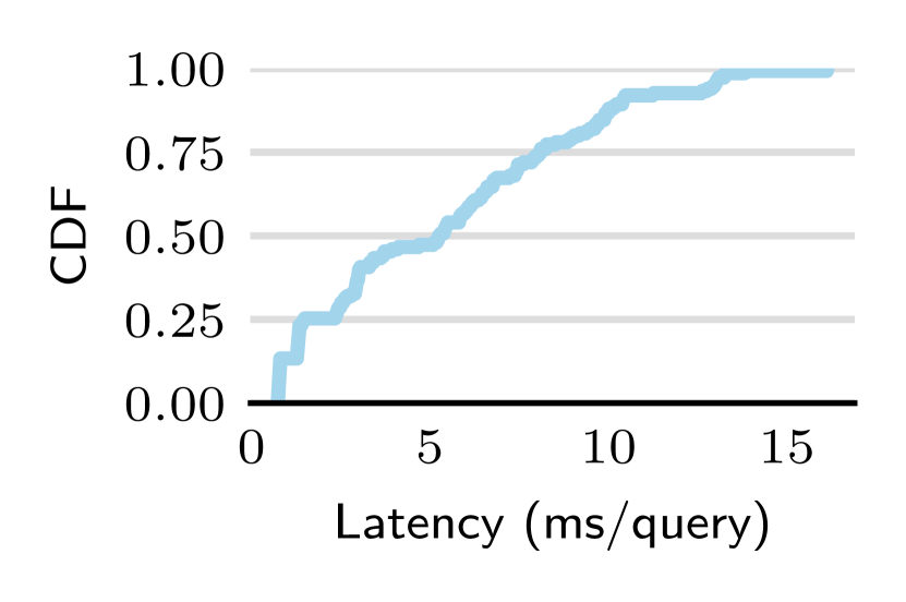
Figure 6(b) shows the latency CDF for routing all 150 queries—the time it takes to check each query against a qd-tree to determine intersecting blocks (Section 3.3). The maximum time it takes for a query is less than 16ms, with most under 10ms. The latencies for checking against the semantic descriptions are not homogeneous, because queries have varying number of filters (of varying complexity).
Robustness. We generated more queries (100 queries per template) using distinct random seeds from before. This enlarged “test” set includes substantially more query literals that the qd-tree did not use for construction. The mean runtime of these 1500 queries on the same qd-tree layout as Figure 5(a) is 7776ms, compared to that figure’s 7752ms, the mean of the 150 “train” queries. This suggests that qd-tree is robust for this templated workload with unseen literals.
7.5. ErrorLogs
We now discuss ErrorLog-Int and ErrorLog-Ext. Table 2 reports the logical metrics for all approaches.
The default range-partitioner (“Baseline”) accesses all tuples. Further, we found that the original feature selection method in Bottom-Up ends up choosing a predicate with very high frequency but also very high selectivity as a feature. It prunes other predicates due to the frequency discount used in the original paper, and its skipping power is poor. Thus, the access ratio is close to . This a weakness of frequency-based feature selection without taking selectivity into account. We tuned it by ignoring predicates with selectivity ¿ . This tuning, which we call , improves the access ratio of Bottom-Up to – (listed in Table 2).
Our greedy qd-tree, on the other hand, achieves excellent skipping capability, accessing only % and % of tuples for ErrorLog-Int and ErrorLog-Ext, respectively. The RL qd-tree improves them to % and % respectively, an up to improvement.
7.5.1. Physical execution
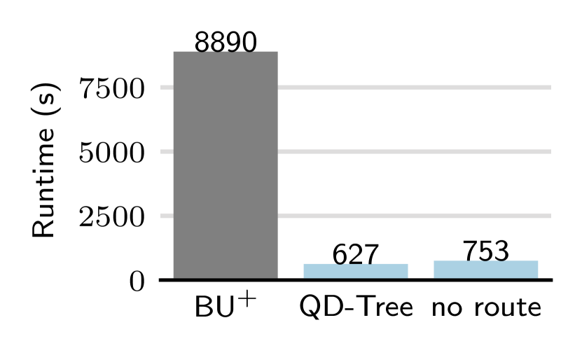
We measure the actual execution runtime for both real datasets on an optimized single-node SparkSQL instance. Each workload consists of queries. Figures 7(a) and (b) show the aggregate runtimes.
We find that qd-tree dominates Bottom-Up+ with a lower runtime for ErrorLog-Int. On ErrorLog-Ext, the speedup becomes because of its higher selectivity. For qd-tree, we report runtimes using qd-tree routing (adding BID IN (...) predicates) and using the default partition pruning (no route). On SparkSQL with Parquet, we observe that qd-tree-based routing is better than no route by % for ErrorLog-Int and % for ErrorLog-Ext.
Figure 7(c) shows the CDF of per-query speedups. We observe that of queries have a speedup of at least (ErrorLog-Int) and (ErrorLog-Ext), respectively. Thus, the excellent skipping benefits reflected in the logical metrics translate well into physical runtime reduction.
Lastly, we executed a subset of the ErrorLog-Int queries on the commercial DBMS. Briefly, the trends remain consistent as before. Query execution with qd-tree query routing is faster than the range-partitioned baseline which needs to touch all blocks. Unlike Parquet, however, we found that no route performed significantly worse than qd-tree routing. We believe this is due to a lack of block-level indexes (dictionaries) for categorical fields, which prevents categorical predicates from pruning blocks in no route.
7.6. Time to Produce Layouts
While quality of data layout is the primary metric of concern in this study, we next discuss the wall-clock time required to produce good data layouts.
TPC-H. Bottom-Up took 71 minutes to produce its layout due to large number of records and queries. It produces a layout only on termination. In contrast, the RL agent Woodblock produces trees immediately and continuously, with quality improving over time. Figure 8 plots the learning curves of Woodblock. There are several key takeaways.
First, at random initialization, Woodblock immediately produces partitioning trees with a scan ratio of . This, in fact, significantly exceeds the quality of the Random partitioner reported in Table 2 (). The reason is that, at initialization Woodblock produces a tree drawn randomly from the search space, which is defined with a candidate cut set extracted from query workload. Leveraging these informative cuts is much better than disregarding workload information.
Second, Woodblock enables the user to explicitly trade-off computation time vs. the quality of layouts produced. As the agent constructs more trees, it learns to bias the cuts that are observed to more profitable, but it also keeps a non-zero probability for exploration. We see that most of the improvement is learned in the first 10 minutes. Further speedups may result from (1) implementing our tree library in a native language rather than in Python, and (2) switching Woodblock’s learning algorithm to a distributed learner (Espeholt et al., 2018).
ErrorLogs. A uniform workload like TPC-H is, in fact, a more challenging task for RL because the uniform distribution of data and queries has higher entropy. On both real ErrorLog workloads, Woodblock produces top-performing trees within 30 seconds (Fig. 8). The run time is much shortened, due to the abundant correlations to be exploited in the real-world data/workload. With the existence of correlations, exploration of the space is significantly faster. On ErrorLog-Int, Greedy and Bottom-Up finished in 12 minutes and 432 minutes, respectively. On ErrorLog-Ext, these numbers became 12 minutes and 565 minutes, respectively.
7.7. Interpreting Learned qd-trees
To gain insights, we now analyze a top-performing qd-tree (constructed by Woodblock) found for the TPC-H workload.
Figure 9 plots the dimensions cut across tree levels. We make a few observations. First, the variety of cuts is high: 8 columns are cut at least 20 times throughout all tree levels. Both categorical (e.g., l_shipmode) and numerical columns (e.g., l_discount) contribute to skipping. This indicates fine-grained cutting, as is done by RL-learned qd-tree, is beneficial. Second, advanced cuts are leveraged (AC; Sec. 6.1), indicating their skippability benefits in complex workloads.
The cuts made at the root and the first two children are:
-
•
p_container IN (LG CASE,LG BOX,LG PACK,LG PKG);
-
•
(First two children) : c_nationkey = s_nationkey.
The next level’s cuts involve l_shipdate and p_brand. Overall, it is clear that existing partitioning techniques (hash or range) do not equate the sophisticated combination of cuts produced by a qd-tree layout.
8. Related Work
Physical Design & Partitioning. Traditionally, data warehouses employ partitioning for the purpose of scaling out computation and load balancing. Data is either chunked into blocks based on arrival time, or partitioned using range or hash partitioning schemes (Larson et al., 2013) or their improvements (Bhattacharjee et al., 2003; Zhou et al., 2012). Our technique may be applied within partitions created by such static schemes. Automated physical design tools provide auto-tuning capabilities based on what-if analyses and integrated into the query optimizer (Agrawal et al., 2004; Agrawal et al., 2006; Rao et al., 2002; Finkelstein et al., 1988; Härder, 1976). AutoAdmin (Agrawal et al., 2004; Agrawal et al., 2006; Zilio et al., 2004; Olma et al., 2017; Pavlo et al., 2012; Wu and Madden, 2011) optimizes a database and its physical design using machine learning and data mining. Some systems perform partitioning based on workload access patterns (Agrawal et al., 2004; Arulraj et al., 2016; Chasseur and Patel, 2013), while other systems are based on graph-based workload modeling techniques (Curino et al., 2010; Quamar et al., 2013; Serafini et al., 2016). Sun et al. (Sun et al., 2014, 2016) (discussed in this paper) extract features from each workload operation based on its predicates. Casper (Athanassoulis et al., 2019) offers a general partitioning design tool based on navigating a three-way tradeoff between read performance, update performance, and memory utilization.
Adaptive Physical Design. The cost of periodic automated physical design can be amortized in an online pay-as-you-go fashion. This line of research can roughly be categorized into two approaches. Online analysis (Bruno and Chaudhuri, 2006, 2007; Schnaitter et al., 2006) uses available system cycles between query execution and offline analysis to optimize physical design. Database cracking (Idreos et al., 2007; Idreos et al., 2011) immediately starts executing queries, and treats each query as a hint to reorganize parts of the data during query processing, usually based on sort attributes. This approach optimizes and adapts the data layout over time.
In contrast, a qd-tree performs data layout using fine-grained descriptions based on a workload set. Our technique learns at coarse-grained time boundaries and emits a synthesized qd-tree data structure to enable data layout. We do not react to individual query execution, but our resulting data structure may be used for continuous ingestion or bulk loading. We find this approach to be suitable for modern data formats such as Parquet, where incremental re-organization is expensive. An interesting direction of future work is to integrate cracking with qd-tree. Since a qd-tree represents a way to layout data, cracking would allow us to incrementally refine the qd-tree over time. A possible approach, left as future work, would be to include the cost of data re-organization into the qd-tree cost model, so that we can enable efficient incremental re-organization over time.
Learned Databases. There is increasing interest in automating core database functionality and design decisions. This line of research leverages recent advancements in deep learning algorithms and scalable hardware (GPU) to improve database systems. Closest to our work is a proposal of learned partition adviser using deep RL (Hilprecht et al., 2019); it focuses on replication and coarse-grained partitioning (e.g., hash) along entire attribute(s), unlike qd-tree which partitions based on a rich set of fine-grained candidate cuts. In this space, machine learning has also been used to revisit tuning (Van Aken et al., 2017), workload forecasting (Ma et al., 2018), data structures and indexes (Kraska et al., 2018; Idreos et al., 2019; Nathan et al., 2020; Ding et al., 2020), and query optimization (Yang et al., 2019; Krishnan et al., 2018; Marcus et al., 2019; Dutt et al., 2019). Our qd-tree may be viewed as a learned physical design or indexing tool: it optimizes for scan-based workloads, common in big data analytics, to minimize the I/O cost of block accesses.
Traditional Indexing. Database indexing is a well-studied space. For one dimensional indexing, B-Trees form the state of the art. Multi-dimensional indexes such as k-d tree (Bentley, 1975) and R-tree (Guttman, 1984) have been proposed to index data over more than one dimension, but they do not adapt to high dimensional data or the specific query workload. These indexes are not a good fit for analytical workloads due to the cost of each index lookup. Modern systems instead use scan-oriented processing over columnar row-groups. Our work may be viewed as workload-aware multi-dimensional indexing adapted to the needs of analytical scan-based workloads.
Partition Pruning. Most scan-oriented databases employ indexing over the blocks to make it easy to skip blocks. Examples include min-max based pruning, also known as small materialized aggregates (SMA) (Moerkotte, 1998), zone maps (Graefe, 2009), and data skipping (Sun et al., 2014, 2016). Here, the system maintains the data distribution information for each block. Depending on the query predicates, these values can be used to determine that a given block might not be needed for a given query. They are commonly employed in systems such as Oracle (Oracle, 2019), Postgres (PostgreSQL, 2019), Microsoft SQL Server (Larson et al., 2013), and Snowflake (Dageville et al., 2016). The most popular SMA is the min-max index, which maintains the minimum and maximum value for each field, per block. Snowflake also maintains SMAs for auto-detected columns in semi-structured data. They are used for simple predicates as well as more complex predicates, such as IN. We leverage such block-level indexes in this paper as well. During query processing, we use a combination of tree routing and SMA indexes to achieve maximum skippability.
9. Conclusion
Running queries at interactive speeds on large datasets is increasingly important. In this paper, we address the problem of best assigning records to data blocks on storage, with a goal to optimize for the important metric of number of blocks accessed by a query. This metric directly relates to the I/O cost, and therefore performance, of most analytical queries. Current techniques based on hash and time-based partitioning or clustering are unable to exploit the workload fully and provide blocks with complete semantic descriptions, which is useful for caching, exploiting additional storage, etc. We propose a new framework called a query-data routing tree, or qd-tree, to address this gap. Further, we develop two novel algorithms for qd-tree construction: one based on a greedy approach and the other based on deep reinforcement learning. Experiments over benchmark and real workloads show that a qd-tree can provide physical speedups of more than an order of magnitude compared to current blocking schemes, and can reach within of the lower bound for data skipping based on selectivity, while providing complete semantic descriptions of created blocks.
References
- (1)
- Agrawal et al. (2006) Sanjay Agrawal, Nicolas Bruno, Surajit Chaudhuri, and Vivek R Narasayya. 2006. AutoAdmin: Self-Tuning Database Systems Technology. IEEE Data Eng. Bull. 29, 3 (2006), 7–15.
- Agrawal et al. (2004) Sanjay Agrawal, Vivek Narasayya, and Beverly Yang. 2004. Integrating Vertical and Horizontal Partitioning into Automated Physical Database Design. In Proceedings of the 2004 ACM SIGMOD International Conference on Management of Data (SIGMOD ’04). ACM, New York, NY, USA, 359–370. https://doi.org/10.1145/1007568.1007609
- Arulraj et al. (2016) Joy Arulraj, Andrew Pavlo, and Prashanth Menon. 2016. Bridging the archipelago between row-stores and column-stores for hybrid workloads. In Proceedings of the 2016 International Conference on Management of Data. 583–598.
- Athanassoulis et al. (2019) Manos Athanassoulis, Kenneth S Bøgh, and Stratos Idreos. 2019. Optimal column layout for hybrid workloads. Proceedings of the VLDB Endowment 12, 13 (2019), 2393–2407.
- Bentley (1975) Jon Louis Bentley. 1975. Multidimensional binary search trees used for associative searching. Commun. ACM 18, 9 (1975), 509–517.
- Bhattacharjee et al. (2003) Bishwaranjan Bhattacharjee, Sriram Padmanabhan, Timothy Malkemus, Tony Lai, Leslie Cranston, and Matthew Huras. 2003. Efficient Query Processing for Multi-Dimensionally Clustered Tables in DB2. In VLDB.
- Bruno and Chaudhuri (2006) Nicolas Bruno and Surajit Chaudhuri. 2006. To tune or not to tune?: a lightweight physical design alerter. In Proceedings of the 32nd international conference on Very large data bases. VLDB Endowment, 499–510.
- Bruno and Chaudhuri (2007) Nicolas Bruno and Surajit Chaudhuri. 2007. An online approach to physical design tuning. In 2007 IEEE 23rd International Conference on Data Engineering. IEEE, 826–835.
- Chasseur and Patel (2013) Craig Chasseur and Jignesh M Patel. 2013. Design and evaluation of storage organizations for read-optimized main memory databases. Proceedings of the VLDB Endowment 6, 13 (2013), 1474–1485.
- Curino et al. (2010) Carlo Curino, Evan Jones, Yang Zhang, and Sam Madden. 2010. Schism: a workload-driven approach to database replication and partitioning. Proceedings of the VLDB Endowment 3, 1-2 (2010), 48–57.
- Dageville et al. (2016) Benoit Dageville, Thierry Cruanes, Marcin Zukowski, Vadim Antonov, Artin Avanes, Jon Bock, Jonathan Claybaugh, Daniel Engovatov, Martin Hentschel, Jiansheng Huang, et al. 2016. The snowflake elastic data warehouse. In Proceedings of the 2016 International Conference on Management of Data. 215–226.
- Ding et al. (2020) Jialin Ding, Umar Farooq Minhas, Jia Yu, Chi Wang, Jaeyoung Do, Yinan Li, Hantian Zhang, Badrish Chandramouli, Johannes Gehrke, Donald Kossmann, David Lomet, and Tim Kraska. 2020. ALEX: An Updatable Adaptive Learned Index. In Proceedings of the 2020 International Conference on Management of Data.
- Dutt et al. (2019) Anshuman Dutt, Chi Wang, Azade Nazi, Srikanth Kandula, Vivek Narasayya, and Surajit Chaudhuri. 2019. Selectivity estimation for range predicates using lightweight models. Proceedings of the VLDB Endowment 12, 9 (2019), 1044–1057.
- Espeholt et al. (2018) Lasse Espeholt, Hubert Soyer, Remi Munos, Karen Simonyan, Vlad Mnih, Tom Ward, Yotam Doron, Vlad Firoiu, Tim Harley, Iain Dunning, Shane Legg, and Koray Kavukcuoglu. 2018. IMPALA: Scalable Distributed Deep-RL with Importance Weighted Actor-Learner Architectures. In Proceedings of the 35th International Conference on Machine Learning (Proceedings of Machine Learning Research), Vol. 80. PMLR, 1407–1416.
- Finkelstein et al. (1988) S. Finkelstein, M. Schkolnick, and P. Tiberio. 1988. Physical Database Design for Relational Databases. ACM Trans. Database Syst. 13, 1 (March 1988), 91–128. https://doi.org/10.1145/42201.42205
- Graefe (2009) Goetz Graefe. 2009. Fast loads and fast queries. In International Conference on Data Warehousing and Knowledge Discovery. Springer, 111–124.
- Guttman (1984) Antonin Guttman. 1984. R-trees: A dynamic index structure for spatial searching. Vol. 14. ACM.
- Härder (1976) Theo Härder. 1976. Selecting an optimal set of secondary indices. In Conference of the European Cooperation in Informatics. Springer, 146–160.
- Hilprecht et al. (2019) Benjamin Hilprecht, Carsten Binnig, and Uwe Röhm. 2019. Towards learning a partitioning advisor with deep reinforcement learning. In Proceedings of the Second International Workshop on Exploiting Artificial Intelligence Techniques for Data Management. 1–4.
- Idreos et al. (2019) Stratos Idreos, Niv Dayan, Wilson Qin, Mali Akmanalp, Sophie Hilgard, Andrew Ross, James Lennon, Varun Jain, Harshita Gupta, David Li, et al. 2019. Design Continuums and the Path Toward Self-Designing Key-Value Stores that Know and Learn. In CIDR.
- Idreos et al. (2007) Stratos Idreos, Martin L Kersten, Stefan Manegold, et al. 2007. Database Cracking. In CIDR, Vol. 7. 68–78.
- Idreos et al. (2011) Stratos Idreos, Stefan Manegold, Harumi Kuno, and Goetz Graefe. 2011. Merging what’s cracked, cracking what’s merged: adaptive indexing in main-memory column-stores. Proceedings of the VLDB Endowment 4, 9 (2011), 586–597.
- Kraska et al. (2018) Tim Kraska, Alex Beutel, Ed H Chi, Jeffrey Dean, and Neoklis Polyzotis. 2018. The case for learned index structures. In Proceedings of the 2018 International Conference on Management of Data. ACM, 489–504.
- Krishnan et al. (2018) Sanjay Krishnan, Zongheng Yang, Ken Goldberg, Joseph Hellerstein, and Ion Stoica. 2018. Learning to optimize join queries with deep reinforcement learning. arXiv preprint arXiv:1808.03196 (2018).
- Larson et al. (2013) Per-Åke Larson, Cipri Clinciu, Campbell Fraser, Eric N. Hanson, Mostafa Mokhtar, Michal Nowakiewicz, Vassilis Papadimos, Susan L. Price, Srikumar Rangarajan, Remus Rusanu, and Mayukh Saubhasik. 2013. Enhancements to SQL server column stores. In Proceedings of the ACM SIGMOD International Conference on Management of Data, SIGMOD 2013, New York, NY, USA, June 22-27, 2013. 1159–1168.
- Liang et al. (2018) Eric Liang, Richard Liaw, Robert Nishihara, Philipp Moritz, Roy Fox, Ken Goldberg, Joseph E. Gonzalez, Michael I. Jordan, and Ion Stoica. 2018. RLlib: Abstractions for Distributed Reinforcement Learning. In International Conference on Machine Learning (ICML).
- Liang et al. (2019) Eric Liang, Hang Zhu, Xin Jin, and Ion Stoica. 2019. Neural Packet Classification. In Proceedings of the ACM Special Interest Group on Data Communication (SIGCOMM ’19). ACM, New York, NY, USA, 256–269. https://doi.org/10.1145/3341302.3342221
- Ma et al. (2018) Lin Ma, Dana Van Aken, Ahmed Hefny, Gustavo Mezerhane, Andrew Pavlo, and Geoffrey J Gordon. 2018. Query-based workload forecasting for self-driving database management systems. In Proceedings of the 2018 International Conference on Management of Data. 631–645.
- Marcus et al. (2019) Ryan Marcus, Parimarjan Negi, Hongzi Mao, Chi Zhang, Mohammad Alizadeh, Tim Kraska, Olga Papaemmanouil, and Nesime Tatbul. 2019. Neo: A Learned Query Optimizer. PVLDB 12, 11 (2019), 1705–1718.
- Moerkotte (1998) Guido Moerkotte. 1998. Small materialized aggregates: A light weight index structure for data warehousing. (1998).
- Moritz et al. (2018) Philipp Moritz, Robert Nishihara, Stephanie Wang, Alexey Tumanov, Richard Liaw, Eric Liang, Melih Elibol, Zongheng Yang, William Paul, Michael I Jordan, et al. 2018. Ray: A distributed framework for emerging AI applications. In 13th USENIX Symposium on Operating Systems Design and Implementation (OSDI 18). 561–577.
- Nathan et al. (2020) Vikram Nathan, Jialin Ding, Mohammad Alizadeh, and Tim Kraska. 2020. Learning Multi-dimensional Indexes. In Proceedings of the 2020 International Conference on Management of Data.
- Olma et al. (2017) Matthaios Olma, Manos Karpathiotakis, Ioannis Alagiannis, Manos Athanassoulis, and Anastasia Ailamaki. 2017. Slalom: Coasting through raw data via adaptive partitioning and indexing. Proceedings of the VLDB Endowment 10, 10 (2017), 1106–1117.
- OpenAI (2018) OpenAI. 2018. OpenAI Five. https://blog.openai.com/openai-five/.
- Oracle (2019) Oracle. 2019. https://oracle.com/.
- Pavlo et al. (2012) Andrew Pavlo, Carlo Curino, and Stanley Zdonik. 2012. Skew-aware automatic database partitioning in shared-nothing, parallel OLTP systems. In Proceedings of the 2012 ACM SIGMOD International Conference on Management of Data. 61–72.
- PostgreSQL (2019) PostgreSQL. 2019. https://www.postgresql.org/.
- Powell (2007) Warren B Powell. 2007. Approximate Dynamic Programming: Solving the curses of dimensionality. Vol. 703. John Wiley & Sons.
- Powell (2016) Warren B Powell. 2016. Perspectives of approximate dynamic programming. Annals of Operations Research 241, 1-2 (2016), 319–356.
- Quamar et al. (2013) Abdul Quamar, K Ashwin Kumar, and Amol Deshpande. 2013. SWORD: scalable workload-aware data placement for transactional workloads. In Proceedings of the 16th International Conference on Extending Database Technology. 430–441.
- Rao et al. (2002) Jun Rao, Chun Zhang, Nimrod Megiddo, and Guy Lohman. 2002. Automating Physical Database Design in a Parallel Database. In Proceedings of the 2002 ACM SIGMOD International Conference on Management of Data (SIGMOD ’02). ACM, New York, NY, USA, 558–569. https://doi.org/10.1145/564691.564757
- Schnaitter et al. (2006) Karl Schnaitter, Serge Abiteboul, Tova Milo, and Neoklis Polyzotis. 2006. Colt: continuous on-line tuning. In Proceedings of the 2006 ACM SIGMOD international conference on Management of data. 793–795.
- Schulman et al. (2017) John Schulman, Filip Wolski, Prafulla Dhariwal, Alec Radford, and Oleg Klimov. 2017. Proximal policy optimization algorithms. arXiv preprint arXiv:1707.06347 (2017).
- Serafini et al. (2016) Marco Serafini, Rebecca Taft, Aaron J Elmore, Andrew Pavlo, Ashraf Aboulnaga, and Michael Stonebraker. 2016. Clay: Fine-grained adaptive partitioning for general database schemas. Proceedings of the VLDB Endowment 10, 4 (2016), 445–456.
- Sun et al. (2014) Liwen Sun, Michael J. Franklin, Sanjay Krishnan, and Reynold S. Xin. 2014. Fine-grained partitioning for aggressive data skipping. In International Conference on Management of Data, SIGMOD 2014, Snowbird, UT, USA, June 22-27, 2014. 1115–1126.
- Sun et al. (2016) Liwen Sun, Michael J. Franklin, Jiannan Wang, and Eugene Wu. 2016. Skipping-oriented Partitioning for Columnar Layouts. PVLDB 10, 4 (2016), 421–432. https://doi.org/10.14778/3025111.3025123
- Van Aken et al. (2017) Dana Van Aken, Andrew Pavlo, Geoffrey J Gordon, and Bohan Zhang. 2017. Automatic database management system tuning through large-scale machine learning. In Proceedings of the 2017 ACM International Conference on Management of Data. 1009–1024.
- Wu and Madden (2011) Eugene Wu and Samuel Madden. 2011. Partitioning techniques for fine-grained indexing. In 2011 IEEE 27th International Conference on Data Engineering. IEEE, 1127–1138.
- Yang et al. (2020) Zongheng Yang, Badrish Chandramouli, Chi Wang, Johannes Gehrke, Yinan Li, Umar Farooq Minhas, Per-Åke Larson, Donald Kossmann, and Rajeev Acharya. 2020. Qd-tree: Learning Data Layouts for Big Data Analytics. Technical Report. Microsoft Research, https://aka.ms/qdtree-tr.
- Yang et al. (2019) Zongheng Yang, Eric Liang, Amog Kamsetty, Chenggang Wu, Yan Duan, Xi Chen, Pieter Abbeel, Joseph M Hellerstein, Sanjay Krishnan, and Ion Stoica. 2019. Deep Unsupervised Cardinality Estimation. Proceedings of the VLDB Endowment 13, 3, 279–292.
- Zhou et al. (2012) Jingren Zhou, Nicolas Bruno, and Wei Lin. 2012. Advanced Partitioning Techniques for Massively Distributed Computation. In Proceedings of the 2012 ACM SIGMOD International Conference on Management of Data (SIGMOD ’12). ACM, New York, NY, USA, 13–24.
- Zilio et al. (2004) Daniel C Zilio, Jun Rao, Sam Lightstone, Guy Lohman, Adam Storm, Christian Garcia-Arellano, and Scott Fadden. 2004. DB2 design advisor: integrated automatic physical database design. In Proceedings of the Thirtieth international conference on Very large data bases-Volume 30. 1087–1097.