An adaptive finite element DtN method for the open cavity scattering problems

Abstract.

Consider the scattering of a time-harmonic electromagnetic plane wave by an open cavity which is embedded in a perfectly electrically conducting infinite ground plane. This paper concerns the numerical solutions of the open cavity scattering problems in both transverse magnetic and transverse electric polarizations. Based on the Dirichlet-to-Neumann (DtN) map for each polarization, a transparent boundary condition is imposed to reduce the scattering problem equivalently into a boundary value problem in a bounded domain. An a posteriori error estimate based adaptive finite element DtN method is proposed. The estimate consists of the finite element approximation error and the truncation error of the DtN operator, which is shown to decay exponentially with respect to the truncation parameter. Numerical experiments are presented for both polarizations to illustrate the competitive behavior of the adaptive method.

1. Introduction

Consider the electromagnetic scattering of a time-harmonic plane wave by an open cavity, which is referred to as a bounded domain embedded in the ground with its opening aligned with the ground surface. The open cavity scattering problems have significant applications in industry and military. In computational and applied electromagnetics, one of the physical parameter of interests is the radar cross section (RCS), which measures the detectability of a target by a radar system. It is crucial to have a deliberate control in the form of enhancement or reduction of the RCS of a target in the stealth technology. The cavity RCS caused by jet engine inlet ducts or cavity-backed patch or slot antennas can dominate the total RCS of an aircraft or a device. It is indispensable to have a thorough understanding of the electromagnetic scattering characteristic of a target, particularly a cavity, in order to successfully implement any desired control of its RCS.

Due to the important applications, the open cavity scattering problems have received much attention by many researchers in both of the engineering and mathematics communities. The time-harmonic problems of cavity-backed apertures with penetrable material filling the cavity interior were introduced and studied initially by researchers in the engineering community [19, 27, 21]. The mathematical analysis for the well-posedness of the variational problems can be found in [1, 2, 3], where the non-local transparent boundary conditions, based on the Fourier transform, were proposed on the open aperture of the cavity. It has been realized that the phenomena of electromagnetic scattering by cavities not only have striking physics but also give rise to many interesting mathematical problems. As more people work on this subject, there has been a rapid development of the mathematical theory and computational methods for the open cavity scattering problems. The stability estimates with explicit dependence on the wavenumber were obtained in [9, 10]. Various analytical and numerical methods have been proposed to solve the challenging large cavity problem [6, 11, 8, 30, 22]. The overfilled cavity problems, where the filling material inside the cavity may protrude into the space above the ground surface, were investigated in [14, 15, 25, 29], where the transparent boundary conditions, based on the Fourier series, were introduced on a semi-circle enclosing the cavity and filling material. The multiple cavity scattering problem was examined in [24, 33], where the cavity is assumed to be composed of finitely many disjoint components. The mathematical analysis can be found in [7, 12] on the related scattering problems in a locally perturbed half-plane. We refer to the survey [23] and the references cited therein for a comprehensive account on the modeling, analysis, and computation of the open cavity scattering problems.

There are two challenges for the open cavity scattering problems: the problems are formulated in unbounded domains; the solutions may have singularities due to possible nonsmooth surfaces and discontinuous media. In this paper, we present an adaptive finite element method with transparent boundary condition to overcome the difficulties.

The first issue concerns the domain truncation. The unbounded physical domain needs to be truncated into a bounded computational domain. An appropriate boundary condition is required on the artificial boundary of the truncated domain to avoid unwanted wave reflection. Such a boundary condition is known as a transparent boundary condition (TBC). There are two different TBCs for the open cavity scattering problems. For a regular open cavity, where the filling material is inside the cavity, the Fourier transform based TBC is imposed on the open aperture of the cavity; for an overfilled cavity, where the filling material appears to protrude out of the cavity through the open aperture into the space above the ground surface, the Fourier series based TBC is imposed on the semi-circle enclosing the cavity and the protruding part. The latter is adopted in this work since it can be used to handle more general open cavities. We refer to the perfectly matched layer (PML) techniques [33, 34] and the method of boundary integral equations [5] as alternative approaches for dealing with the issue of the unbounded domains of the open cavity scattering problems.

Due to the existence of corners of cavities or the discontinuity of the dielectric coefficient for the filling material, the solutions have singularites that slow down the convergence of the finite element for uniform mesh refinements. The second issue can be resolved by using the a posteriori error estimate based adaptive finite element method. The a posteriori error estimates are computable quantities from numerical solutions. They measure the solution errors of discrete problems without requiring any a priori information of exact solutions. It is known that the meshes and the associated numerical complexity are quasi-optimal for appropriately designed adaptive finite element methods.

The goal of this paper is to combine the adaptive finite element method and the transparent boundary conditions to solve the open cavity scattering problems in an optimal fashion. Specifically, we consider the scattering of a time-harmonic electromagnetic plane wave by an open cavity embedded in an infinite ground plane. Throughout, the medium is assumed to be constant in the $x_{3}$ direction. The ground plane and the cavity wall are assumed to be perfect electric conductors. The cavity is filled with a nonmagnetic and possibly inhomogeneous material, which may protrude out of the cavity to the upper half-space in a finite extend. The infinite upper half-space above the ground plane and the protruding part of the cavity is composed of a homogeneous medium. Two fundamental polarizations, transverse magnetic (TM) and transverse electric (TE), are studied. In this setting, the three-dimensional Maxwell equations may be reduced to the two dimensional Helmholtz equation and generalized Helmholtz equation for TM and TE polarizations, respectively. Based on the Dirichlet-to-Neumann (DtN) map for each polarization, a transparent boundary condition is imposed to reduce the scattering problem equivalently into a boundary value problem in a bounded domain. The nonlocal DtN operator is defined as an infinite Fourier series which needs to be truncated into a sum of finitely many terms in actual computation. The a posteriori error estimate is derived bewteen the solution of original scattering problem and the finite element solution of the discrete problem with the truncated DtN operator. The error estimate takes account of the finite element discretization error and the truncation error of the DtN operator. Using the asymptotic properties of the solution and DtN operator, we consider a dual problem for the error and show that the truncation error of the DtN operator decays exponentially respect to the truncation parameter, which implies that the truncation number does not need to be large. Numerical experiments are presented for both polarization cases to demonstrate the effectiveness of the proposed adaptive method. The related work can be found in [16, 17, 18, 31] on the adaptive finite element DtN method for solving other scattering problems in open domains.

The paper is organized as follows. Section 2 concerns the problem formulation. The three-dimensional Maxwell equations are introduced and reduced into the two-dimensional Helmholtz equation under the two fundamental modes: transverse magnetic (TM) polarization and transverse electric (TE) polarization. Sections 3 and 4 are devoted to the TM and TE polarizations, respectively. In each section, the variational problem and its finite element approximation are introduced; the a posteriori error analysis is given for the discrete problem with the truncated DtN operator; the adaptive finite element algorithm is presented. In Section 5, the stiff matrix is constructed for the the TBC part of the sesquilinear form. Section 6 describes the formulas of the backscatter radar cross section (RCS). Section 7 presents some numerical examples to illustrate the advantages of the proposed method. The paper is concluded with some general remarks and directions for future research in Section 8.

2. Problem formulation

Consider the electromagnetic scattering by an open cavity, which is a bounded domain embedded in the ground with its opening aligned with the ground surface. By assuming the time dependence $e^{-{\rm i}\omega t}$, the electromagnetic wave propagation is governed by the time-harmonic Maxwell equations

$$\nabla\times\boldsymbol{E}={\rm i}\omega\boldsymbol{B},\quad\nabla\times\boldsymbol{H}=-{\rm i}\omega\boldsymbol{D}+\boldsymbol{J},$$ (2.1)

where $\boldsymbol{E}$ is the electric field, $\boldsymbol{H}$ is the magnetic field, $\boldsymbol{B}$ is the magnetic flux density, $\boldsymbol{D}$ is the electric flux density, $\boldsymbol{J}$ is the electric current density, and $\omega>0$ is the angular frequency. For a linear medium, the constitutive relations, describing the macroscopic properties of the medium, are given by

$$\boldsymbol{B}=\mu\boldsymbol{H},\quad\boldsymbol{D}=\epsilon\boldsymbol{E},\quad\boldsymbol{J}=\sigma\boldsymbol{E},$$ (2.2)

where $\mu$ is the magnetic permeability, $\epsilon$ is the electric permittivity, and $\sigma$ is the electrical conductivity. Throughout, the medium is assumed to be non-magnetic, i.e., the magnetic permeability $\mu$ is a constant everywhere, but the electric permittivity $\epsilon$ and the electrical conductivity $\sigma$ are allowed to be spatial variable functions. Substituting (2.2) into (2.1) leads to a coupled system for the electric and magnetic fields

$$\nabla\times\boldsymbol{E}={\rm i}\omega\mu\boldsymbol{H},\quad\nabla\times\boldsymbol{H}=-{\rm i}\omega\epsilon\boldsymbol{E}+\sigma\boldsymbol{E}$$ (2.3)

Eliminating the magnetic field from (2.3), we may obtain the Maxwell system for the electric field

$$\nabla\times(\nabla\times\boldsymbol{E})-\kappa^{2}\boldsymbol{E}=0,$$ (2.4)

where the wavenumber $\kappa=(\omega^{2}\epsilon\mu+{\rm i}\omega\mu\sigma)^{1/2},\Im\kappa\geq 0$. Similarly, we may eliminate the electric field and obtain the Maxwell system for the magnetic field

$$\nabla\times(\kappa^{-2}\nabla\times\boldsymbol{H})-\boldsymbol{H}=0.$$ (2.5)

When the cavity has a constant cross section along the $x_{3}$-axis and the plane of incidence is in the $x_{1}x_{2}$-plane, as a consequence, the electromagnetic fields are independent of the $x_{3}$ variable. The three-dimensional Maxwell equations can be reduced to either the two-dimensional Helmholtz equation or the two-dimensional generalized Helmholtz equation.

Let $D\subset\mathbb{R}^{2}$ be the cross section of the $x_{3}$-invariant cavity with a Lipschitz continuous boundary $\partial D=S\cup\Gamma$. Here $S$ is the cavity wall and $\Gamma$ is the open aperture of the cavity, which is aligned with the infinite ground plane $\Gamma_{g}$. The cavity is filled with an inhomogeneous medium characterized by the dielectric permittivity $\epsilon$, the magnetic permeability $\mu$, and the electric conductivity $\sigma$. We point out that the inhomogeneous medium filling the cavity may protrude into the space above the ground plane, which is called an overfilled cavity. Let $B_{R}^{+}=\{x\in\mathbb{R}^{2}:|x|<R,\,x_{2}>0\}$ and $B_{\hat{R}}^{+}=\{x\in\mathbb{R}^{2}:|x|<\hat{R},\,x_{2}>0\}$ be upper half-discs with radii $R$ and $\hat{R}$, where $R>\hat{R}>0$. Denote by $\Gamma_{R}^{+}=\{x\in\mathbb{R}^{2}:|x|=R,x_{2}>0\}$ and $\Gamma_{\hat{R}}^{+}=\{x\in\mathbb{R}^{2}:|x|=\hat{R},x_{2}>0\}$ the upper semi-circles. The radius $\hat{R}$ can be taken to be sufficiently large such that the open exterior domain $\mathbb{R}^{2}_{+}\setminus B_{\hat{R}}^{+}$ is filled with a homogeneous medium with constant permittivity $\epsilon=\epsilon_{0}$ and zero conductivity $\sigma=0$. Let $\Omega=B_{R}^{+}\cup D$ be the bounded domain where our reduced boundary value problems are formulated. The problem geometry is shown in Figure 1.

Figure 1. Problem geometry of the electromagnetic scattering by an open cavity.

Since the structure is invariant in the $x_{3}$-axis, we consider two fundamental polarizations for the electromagnetic fields: transverse magnetic (TM) polarization and transverse electric (TE) polarization. In TM case, the magnetic field is perpendicular to the plane of incidence and does not have the component in the $x_{3}$-axis; the electric field, being perpendicular to the magnetic field and lying in the $x_{1}x_{2}$-plane, is invariant in the $x_{3}$-axis and takes the form $\boldsymbol{E}(x_{1},x_{2})=(0,0,u(x_{1},x_{2}))$, where $u$ is a scalar function. It is easy to verify from (2.4) that $u$ satisfies the Helmholtz equation

$$\Delta u+\kappa^{2}u=0\quad\text{in}~{}\mathbb{R}^{2}_{+}\cup D.$$ (2.6)

In TE case, the electromagnetic fields are characterized by its electric field being perpendicular to the plane of incidence and contain no electric field component in the $x_{3}$-axis. The magnetic field, being perpendicular to the electric field and lying in the $x_{1}x_{2}$-plane, is invariant in the $x_{3}$-axis and has the form $\boldsymbol{H}(x_{1},x_{2})=(0,0,u(x_{1},x_{2}))$, where $u$ is also a scalar function. It follows from (2.5) that $u$ satisfies the generalized Helmholtz equation

$$\nabla\cdot(\kappa^{-2}\nabla u)+u=0\quad\text{in}~{}\mathbb{R}^{2}_{+}\cup D.$$ (2.7)

When the ground plane and the cavity wall are assumed to be perfect conductors, the following perfectly electrically conducting (PEC) boundary condition can be imposed

$$\nu\times\boldsymbol{E}=0\quad\text{on}~{}\Gamma_{g}\cup S,$$ (2.8)

where $\nu$ is the unit normal vector to $\Gamma_{g}$ and $S$. In TM polarization, the PEC boundary condition (2.8) reduces to the homogeneous Dirichlet boundary condition

$$u=0\quad\text{on}~{}\Gamma_{g}\cup S.$$ (2.9)

In TE polarization, the PEC boundary condition (2.8) reduces to the homogeneous Neumann boundary condition

$$\partial_{\nu}u=0\quad\text{on}~{}\Gamma_{g}\cup S.$$ (2.10)

In this paper, we consider the numerical solutions and present an adaptive finite element DtN method for both of the TM problem (2.6), (2.9) and the TE problem (2.7), (2.10). The more complicated three-dimensional Maxwell equations will be our future work.

3. TM polarization

In this section, we discuss the TM polarization and study its finite element approximation. The a posteriori analysis is carried out for both the finite element discretization error and the DtN operator truncation error. An adaptive finite element DtN method is presented for the truncated discrete problem.

3.1. Variational problem

In TM polarization, the nonzero component of the electric field $u$ satisfies the boundary value problem

$$\begin{cases}\Delta u+\kappa^{2}u=0\quad&{\rm in}~{}\mathbb{R}^{2}_{+}\cup D,\\ u=0\quad&{\rm on}~{}\Gamma_{g}\cup S.\end{cases}$$ (3.1)

Since the problem is imposed in the open domain, a radiation condition is required to complete the formulation.

Consider the incidence of a plane wave

$$u^{\rm i}(x_{1},x_{2})=e^{{\rm i}(\alpha x_{1}-\beta x_{2})},$$

which is sent from the above to impinge the cavity. Here $\alpha=\kappa_{0}\sin\theta,\beta=\kappa_{0}\cos\theta$, $\theta\in\left(-\frac{\pi}{2},\frac{\pi}{2}\right)$ is the incident angle, and $\kappa_{0}=\omega(\epsilon_{0}\mu)^{1/2}$ is the wavenumber in the free space $\mathbb{R}^{2}_{+}\setminus B_{R}^{+}$. It is easy to verify from (2.9) that the reflected wave is

$$u^{\rm r}(x_{1},x_{2})=-e^{{\rm i}(\alpha x_{1}+\beta x_{2})}.$$

By the Jacobi–Anger identity, the incident and reflected waves admit the following expansions:

$$u^{\rm i}(x)=J_{0}(\kappa_{0}r)+2\sum\limits_{n=1}^{\infty}{\rm i}^{n}J_{n}(\kappa_{0}r)\cos n(\theta-\pi/2-\phi)$$ (3.2)

and

$$u^{\rm r}(x)=-J_{0}(\kappa_{0}r)-2\sum\limits_{n=1}^{\infty}{\rm i}^{n}J_{n}(\kappa_{0}r)\cos n(\theta-\pi/2+\phi),$$ (3.3)

where $J_{n}$ is the Bessel function of the first kind with order $n$ and $x=r(\cos\phi,\sin\phi)$ with $\phi$ being the observation angle. Define the reference wave $u^{\rm ref}=u^{\rm i}+u^{\rm r}$. It follows from (3.2)–(3.3) that

$$u^{\rm ref}(x)=\sum\limits_{n=1}^{\infty}4{\rm i}^{n}J_{n}(\kappa_{0}r)\sin n(\theta-\pi/2)\sin n\phi.$$ (3.4)

The total field $u$ consists of the reference field $u^{\rm ref}$ and the scattered field $u^{\rm s}$, i.e.,

$$u=u^{\rm ref}+u^{\rm s},$$ (3.5)

where the scattered field $u^{\rm s}$ is required to satisfy the Sommerfeld radiation condition

$$\lim_{r=|x|\to\infty}r^{1/2}(\partial_{r}u^{\rm s}-{\rm i}\kappa_{0}u^{\rm s})=0.$$

Let $L_{\rm TM}^{2}(\Gamma_{R}^{+}):=\left\{u\in L^{2}(\Gamma_{R}^{+}):u(R,0)=u(R,\pi)=0\right\}$. For any $u\in L_{\rm TM}^{2}(\Gamma_{R}^{+})$, it has the Fourier series expansion

$$u(R,\phi)=\sum\limits_{n=1}^{\infty}a_{n}\sin n\phi,\quad a_{n}=\frac{2}{\pi}\int_{0}^{\pi}u(R,\phi)\sin n\phi\,{\rm d}\phi.$$

Define the trace function space $H_{\rm TM}^{s}(\Gamma_{R}^{+}):=\left\{u\in L_{\rm TM}^{2}(\Gamma_{R}^{+}):\|u\|_{H_{\rm TM}^{s}(\Gamma_{R}^{+})}\leq\infty\right\},$ where the $H_{\rm TM}^{s}(\Gamma_{R}^{+})$ norm is given by

$$\|u\|_{H^{s}_{\rm TM}(\Gamma_{R}^{+})}=\left(\sum\limits_{n=1}^{\infty}(1+n^{2})^{s}|a_{n}|^{2}\right)^{1/2}.$$

It is clear that the dual space of $H_{\rm TM}^{s}(\Gamma_{R}^{+})$ is $H_{\rm TM}^{-s}(\Gamma_{R}^{+})$ with respect to the scalar product in $L^{2}(\Gamma_{R}^{+})$ given by

$$\langle u,v\rangle_{\Gamma_{R}^{+}}=\int_{\Gamma_{R}^{+}}u\overline{v}\,{\rm d}s.$$

As discussed in [23], a DtN operator is introduced on $\Gamma_{R}^{+}$:

$$(B_{\rm TM}u)(R,\phi)=\kappa_{0}\sum\limits_{n=1}^{\infty}\frac{H_{n}^{(1)^{\prime}}(\kappa_{0}R)}{H_{n}^{(1)}(\kappa_{0}R)}a_{n}\sin n\phi,$$ (3.6)

where $H_{n}^{(1)}$ is the Hankel function of the first kind with order $n$. It is shown in [29, Lemma 3.1] that $B_{\rm TM}:H^{1/2}_{\rm TM}(\Gamma_{R}^{+})\rightarrow H_{TM}^{-1/2}(\Gamma_{R}^{+})$ is continuous. The TBC can be imposed for the total field as follows:

$$\partial_{\rho}u=B_{\rm TM}u+f\quad{\rm on}~{}\Gamma_{R}^{+},$$

where $f=\partial_{\rho}u^{\rm ref}-B_{\rm TM}u^{\rm ref}$. Substituting (3.4) into (3.6) and applying the Wronskian identity, we obtain explicitly

$$f=-\frac{8}{\pi R}\sum\limits_{n=1}^{\infty}\frac{{\rm i}^{n+1}}{H_{n}^{(1)}(\kappa_{0}R)}\sin n(\theta-\pi/2)\sin n\phi.$$

The original cavity scattering problem (3.1) can be reduced equivalently into the boundary value problem

$$\begin{cases}\Delta u+k^{2}u=0\quad&{\rm in}~{}\Omega,\\ u=0\quad&{\rm on}~{}S\cup\Gamma_{g},\\ \partial_{\rho}u-B_{\rm TM}u=f\quad&{\rm on}~{}\Gamma_{R}^{+},\end{cases}$$

which has the variational formulation: find $u\in H_{0}^{1}(\Omega):=\left\{u\in H^{1}(\Omega):u=0~{}{\rm on}~{}S\cup\Gamma_{g}\right\}$ such that

$$a_{\rm TM}(u,v)=\int_{\Gamma_{R}^{+}}f\bar{v}\,{\rm d}s\qquad\forall\,v\in H_{0}^{1}(\Omega).$$ (3.7)

Here the sesquilinear form $a_{\rm TM}:H_{0}^{1}(\Omega)\times H_{0}^{1}(\Omega)\to\mathbb{C}$ is defined as

$$a_{\rm TM}(u,v)=\int_{\Omega}\nabla u\cdot\nabla\bar{v}\,{\rm d}x-\int_{\Omega}\kappa^{2}u\bar{v}\,{\rm d}x-\int_{\Gamma_{R}^{+}}B_{\rm TM}u\,\bar{v}\,{\rm d}s.$$

The following theorem of the well-posedness of the variational problem (3.7) is proved in [23].

Theorem 3.1.

The variational problem (3.7) has a unique solution $u\in H_{0}^{1}(\Omega)$, which satisfies the estimate

$$\|u\|_{H^{1}(\Omega)}\lesssim\|f\|_{H^{-1/2}(\Gamma^{+}_{R})}.$$

Hereafter, the notation $a\lesssim b$ stands for $a\leq Cb$, where $C$ is a positive constant whose value is not required but should be clear from the context.

3.2. Finite element approximation

Let $\mathcal{M}_{h}$ be a regular triangulation of $\Omega$, where $h$ denotes the maximum diameter of all the elements in $\mathcal{M}_{h}$. To avoid being distracted from the main focus of the a posteriori error analysis, we assume for simplicity that $S$ and $\Gamma_{R}^{+}$ are polygonal to keep from using the isoparametric finite element space and deriving the approximation error of the boundaries $S$ and $\Gamma_{R}^{+}$. Thus any edge $e\in\mathcal{M}_{h}$ is a subset of $\partial\Omega$ if it has two boundary vertices.

Let $V_{h}\subset H_{0}^{1}(\Omega)$ be a conforming finite element space, i.e.,

$$V_{h}:=\left\{v_{h}\in C(\overline{\Omega}):v_{h}|_{T}\in P_{m}(K)~{}\forall\,T\in\mathcal{M}_{h},v_{h}=0~{}{\rm on}~{}S\cup\Gamma_{g}\right\}.$$

In practice, the DtN operator (3.6) needs to be truncated into a sum of finitely many terms

$$B_{\rm TM}^{N}u=\kappa_{0}\sum\limits_{n=1}^{N}\frac{H_{n}^{(1)^{\prime}}(\kappa_{0}R)}{H_{n}^{(1)}(\kappa_{0}R)}a_{n}\sin n\phi,\quad a_{n}=\frac{2}{\pi}\int_{0}^{\pi}u(R,\phi)\sin n\phi\,{\rm d}\phi.$$ (3.8)

Taking account of the DtN operator truncation, we obtain the finite element approximation to the variational problem (3.7): find $u_{h}\in V_{h}$ such that

$$a_{\rm TM}^{N}(u^{h},v^{h})=\int_{\Gamma_{R}^{+}}f\,\overline{v^{h}}\,{\rm d}s\quad\forall~{}v_{h}\in V_{h},$$ (3.9)

where the sesquilinear form $a_{\rm TM}^{N}:V_{h}\times V_{h}\to\mathbb{C}$ is

$$a_{\rm TM}^{N}(u^{h},v^{h})=\int_{\Omega}\nabla u^{h}\cdot\nabla\overline{v^{h}}\,{\rm d}x-\int_{\Omega}\kappa^{2}u^{h}\,\overline{v^{h}}\,{\rm d}x-\int_{\Gamma_{R}^{+}}B_{\rm TM}^{N}u^{h}\,\overline{v^{h}}\,{\rm d}s.$$

For sufficiently small $h$ and sufficiently large $N$, the discrete inf-sup condition of the sesquilinear form $a_{\rm TM}^{N}$ can be established by an argument of Schatz [28]. It follows from the general theory in [4] that the truncated variational problem (3.9) admits a unique solution. Since our focus is the a posteriori error estimate and the associated adaptive algorithm, we assume that the discrete problem (3.9) has a unique solution $u_{h}\in V_{h}$.

3.3. A posteriori error analysis

For any triangular element $T\in\mathcal{M}_{h}$, denoted by $h_{T}$ its diameter. Let $\mathcal{B}_{h}$ denote the set of all the edges of $T$. For any edge $e\in\mathcal{B}_{h}$, denote by $h_{e}$ its length. For any interior edge $e$, which is the common side of triangular elements $T_{1},T_{2}\in\mathcal{M}_{h}$, we define the jump residual across $e$ as

$$J_{e}=-\big{(}\nabla u^{h}|_{T_{1}}\cdot\nu_{1}+\nabla u^{h}|_{T_{2}}\cdot\nu_{2}\big{)},$$

where $\nu_{j}$ is the unit outward normal vector on the boundary of $T_{j},j=1,2$. For any boundary edge $e\subset\Gamma_{R}^{+}$, the jump residual is defined as

$$J_{e}=2\big{(}B_{\rm TM}^{N}u^{h}-\nabla u^{h}\cdot\nu-f\big{)}.$$

For any triangle $T\in\mathcal{M}_{h}$, denote by $\eta_{T}$ the local error estimator as follows:

$$\eta_{T}=h_{T}\|H_{\rm TM}u^{h}\|_{L^{2}(T)}+\bigg{(}\frac{1}{2}\sum\limits_{e\in\partial T}h_{e}\|J_{e}\|_{L^{2}(e)}^{2}\bigg{)}^{1/2}$$

where $H_{\rm TM}$ is the Helmholtz operator defined by $H_{\rm TM}u=\Delta u+\kappa^{2}u$.

Let $\xi=u-u^{h}$, where $u$ and $u_{h}$ are the solutions of the variational problems (3.7) and (3.9), respectively. Introduce a dual problem: find $w\in H_{0}^{1}(\Omega)$ such that

$$a_{\rm TM}(v,w)=\int_{\Omega}v\bar{\xi}\,{\rm d}x\quad\forall v\in H_{0}^{1}(\Omega).$$ (3.10)

It is easy to check that $w$ is the solution of the following boundary value problem:

$$\begin{cases}\Delta w+\kappa^{2}w=-\xi\quad&{\rm in}~{}\Omega,\\ w=0\quad&{\rm on}~{}S\cup\Gamma_{g},\\ \partial_{\rho}w=B_{\rm TM}^{*}w\quad&{\rm on}~{}\Gamma_{R}^{+},\end{cases}$$

where $B_{\rm TM}^{*}$ is the adjoint operator of $B_{\rm TM}$ and is given by

$$B_{\rm TM}^{*}u=\kappa_{0}\sum\limits_{n=1}^{\infty}\overline{\left(\frac{H_{n}^{(1)^{\prime}}(\kappa_{0}R)}{H_{n}^{(1)}(\kappa_{0}R)}\right)}a_{n}\sin n\phi,\quad a_{n}=\frac{2}{\pi}\int_{0}^{\pi}u(R,\phi)\sin n\phi\,{\rm d}\phi.$$

The following three lemmas are proved in [17], where the first lemma concerns the well-posedness of the dual problem, the second lemma gives the trace result in $H_{0}^{1}(\Omega)$, and the third lemma shows the error representation formulas.

Lemma 3.2.

The dual problem (3.10) has a unique solution $w\in H^{1}_{0}(\Omega)$, which satisfies the estimate

$$\|w\|_{H^{1}(\Omega)}\lesssim\|\xi\|_{L^{2}(\Omega)}.$$

Lemma 3.3.

For any $u\in H_{0}^{1}(\Omega)$, the following estimates hold:

$$\|u\|_{H^{1/2}(\Gamma_{R}^{+})}\lesssim\|u\|_{H^{1}(\Omega)},\quad\|u\|_{H^{1/2}(\Gamma_{\hat{R}}^{+})}\lesssim\|u\|_{H^{1}(\Omega)}.$$

Lemma 3.4.

Let $u,u_{h}$, and $w$ be the solutions to the problems (3.7), (3.9), and (3.10), respectively. The following identities hold:

$$\|\xi\|^{2}_{H^{1}(\Omega)}=\Re\Big{(}a_{\rm TM}(\xi,\xi)+\langle(B_{\rm TM}^{N}-B_{\rm TM})\xi,\xi\rangle_{\Gamma_{R}^{+}}\Big{)}+\Re\langle B^{N}_{\rm TM}\xi,\xi\rangle_{\Gamma_{R}^{+}}+\Re\int_{\Omega}(\kappa^{2}+1)|\xi|^{2}{\rm d}x,$$

$$\|\xi\|^{2}_{L^{2}(\Omega)}=a_{\rm TM}(\xi,w)+\langle(B_{\rm TM}-B_{\rm TM}^{N})\xi,w\rangle_{\Gamma_{R}^{+}}-\langle(B_{\rm TM}-B_{\rm TM}^{N})\xi,w\rangle_{\Gamma_{R}^{+}},$$

$$a_{\rm TM}(\xi,\psi)+\langle(B_{\rm TM}-B^{N}_{\rm TM})\xi,\psi\rangle_{\Gamma_{R}^{+}}=\int_{\Gamma_{R}^{+}}f(\overline{\psi-\psi_{h}})\,{\rm d}s-a_{\rm TM}^{N}(u^{h},\psi-\psi^{h})$$

$$\qquad\qquad\quad+\langle(B_{\rm TM}-B^{N}_{\rm TM})u,\psi\rangle_{\Gamma_{R}^{+}}\quad\forall\,\psi\in H^{1}_{0}(\Omega),\psi_{h}\in V_{h}.$$

The following result concerns the truncation error of the DtN operator and plays an important role in the a posteriori error estimate.

Lemma 3.5.

Let $u$ be the solution to (3.7) and $\psi$ be any function in $H^{1}_{0}(\Omega)$. For sufficiently large $N$, the following estimate holds:

$$\left|\langle(B_{\rm TM}-B_{\rm TM}^{N})u,\psi\rangle_{\Gamma_{R}^{+}}\right|\lesssim\bigg{[}\Big{(}\frac{\hat{R}}{R}\Big{)}^{N}+\Big{(}\frac{e\kappa_{0}R}{2N}\Big{)}^{2N+4}\bigg{]}\|u^{\rm ref}\|_{H^{1}(\Omega)}\|\psi\|_{H^{1}(\Omega)}.$$

Proof.

By (3.5), we have $u=u^{\rm s}+u^{\rm ref}$, where $u^{\rm ref}$ is the reference field and $u^{\rm s}$ is the scattered field satisfying the Sommerfeld radiation condition. For sufficiently large $N$, it is shown in [17, Lemma 4] that

$$|\langle(B_{\rm TM}-B_{\rm TM}^{N})u^{\rm s},\psi\rangle_{\Gamma_{R}^{+}}|\lesssim\Big{(}\frac{\hat{R}}{R}\Big{)}^{N}\|u^{\rm s}\|_{H^{1/2}(\Gamma_{R}^{+})}\|\psi\|_{H^{1/2}(\Gamma_{R}^{+})}.$$

A straightforward calculation yields

$$(B_{\rm TM}-B_{\rm TM}^{N})u^{\rm ref}=\kappa_{0}\sum\limits_{n=N+1}^{\infty}\frac{H_{n}^{(1)^{\prime}}(\kappa_{0}R)}{H_{n}^{(1)}(\kappa_{0}R)}\left[4{\rm i}^{n}J_{n}(\kappa_{0}R)\sin n(\theta-\frac{\pi}{2})\right]\sin n\phi.$$

By [32], for sufficiently large $n$, we have

$$J_{n}(z)\sim\frac{1}{\sqrt{2\pi n}}\left(\frac{ez}{2n}\right)^{n},\quad\left|\frac{H_{n}^{(1)^{\prime}}(\kappa_{0}R)}{H_{n}^{(1)}(\kappa_{0}R)}\right|\lesssim n,$$

which give

$$|\langle(B_{\rm TM}-B_{\rm TM}^{N})u^{\rm ref},\psi\rangle|=\frac{\pi}{2}\kappa_{0}\left|\sum\limits_{n=N+1}^{\infty}\frac{H_{n}^{(1)^{\prime}}(\kappa_{0}R)}{H_{n}^{(1)}(\kappa_{0}R)}\left[4{\rm i}^{n}J_{n}(\kappa_{0}R)\sin n(\theta-\frac{\pi}{2})\right]\hat{\psi}_{n}(R)\right|$$

$$\leq 2\pi\kappa_{0}\sum\limits_{n=N+1}^{\infty}\left|\frac{H_{n}^{(1)^{\prime}}(\kappa_{0}R)}{H_{n}^{(1)}(\kappa_{0}R)}\right|\left|J_{n}(\kappa_{0}R)\right||\hat{\psi}_{n}(R)|$$

$$\lesssim 2\pi\kappa_{0}\sum\limits_{n=N+1}^{\infty}n\frac{1}{\sqrt{2\pi n}}\left(\frac{e\kappa_{0}R}{2n}\right)^{n}|\hat{\psi}_{n}(R)|$$

$$\lesssim\sqrt{2\pi}\kappa_{0}\left\{\sum\limits_{n=N+1}^{\infty}\left[\sqrt{n}\frac{1}{\sqrt{2\pi n}}\left(\frac{e\kappa_{0}R}{2n}\right)^{n}\right]^{2}\right\}^{1/2}\left\{\sum\limits_{n=N+1}^{\infty}2\pi\left(1+n^{2}\right)^{1/2}|\hat{\psi}_{n}(R)|^{2}\right\}^{1/2}$$

$$\lesssim\kappa_{0}\left\{\sum\limits_{n=N+1}^{\infty}\left(\frac{e\kappa_{0}R}{2n}\right)^{2n}\right\}^{1/2}\|\psi\|_{H^{1/2}(\Gamma_{R}^{+})}.$$

For $N>\frac{e\kappa_{0}R}{2}$, it is easy to verify

$$\sum\limits_{n=N+1}^{\infty}\left(\frac{e\kappa_{0}R}{2n}\right)^{2n}\leq\sum\limits_{n=N+1}^{\infty}\left(\frac{e\kappa_{0}R}{2N}\right)^{2n}=\frac{\left(\frac{e\kappa_{0}R}{2N}\right)^{2N+4}}{1-\left(\frac{e\kappa_{0}R}{2N}\right)^{2}}.$$

Hence

$$|\langle(B_{\rm TM}-B_{\rm TM}^{N})u^{\rm ref},\psi\rangle| \lesssim \kappa_{0}\frac{\left(\frac{e\kappa_{0}R}{2N}\right)^{2N+4}}{1-\left(\frac{e\kappa_{0}R}{2N}\right)^{2}}\sqrt{2\pi R^{2}}\sqrt{\frac{1}{2\pi R^{2}}}\|\psi\|_{H^{1/2}(\Gamma_{R}^{+})}$$

$$\lesssim \frac{\kappa_{0}}{\sqrt{2\pi}R}\frac{\left(\frac{e\kappa_{0}R}{2N}\right)^{2N+4}}{1-\left(\frac{e\kappa_{0}R}{2N}\right)^{2}}\|u^{\rm ref}\|_{H^{1}(B_{R}^{+})}\|\psi\|_{H^{1}(\Omega)}$$

$$\leq \frac{\kappa_{0}}{\sqrt{2\pi}R}\frac{1}{1-\left(\frac{e\kappa_{0}R}{2N}\right)^{2}}\left(\frac{e\kappa_{0}R}{2N}\right)^{2N+4}\|u^{\rm ref}\|_{H^{1}(\Omega)}\|\psi\|_{H^{1}(\Omega)}.$$

Combining the above estimates, we obtain

$$|\langle(B_{\rm TM}-B_{\rm TM}^{N})u,\psi\rangle|\lesssim\left(\frac{R^{\prime}}{R}\right)^{N}\|u^{\rm s}\|_{H^{1/2}(\Gamma_{R}^{+})}\|\psi\|_{H^{1}(\Omega)}+\left(\frac{e\kappa_{0}R}{2N}\right)^{2N+4}\|u^{\rm ref}\|_{H^{1}(\Omega)}\|\psi\|_{H^{1}(\Omega)}.$$

Since

$$\|u^{s}\|_{H^{1}(\Omega)}=\|u-u^{\rm ref}\|_{H^{1}(\Omega)}\leq\|u\|_{H^{1}(\Omega)}+\|u^{\rm ref}\|_{H^{1}(\Omega)}$$

and

$$\|u\|_{H^{1}(\Omega)}\lesssim\|f\|_{H^{-1/2}(\Gamma_{R}^{+})},$$

it suffices to estimate $f$. A simple calculation yields

$$\|f\|_{H^{-1/2}(\Gamma_{R}^{+})} \leq \|\partial_{\rho}u^{\rm ref}\|_{H^{-1/2}(\Gamma_{R}^{+})}+\|B_{\rm TM}u^{\rm ref}\|_{H^{-1/2}(\Gamma_{R}^{+})}$$

$$\lesssim \|\partial_{\rho}u^{\rm ref}\|_{H^{-1/2}(\Gamma_{R}^{+})}+\|u^{\rm ref}\|_{H^{1/2}(\Gamma_{R}^{+})}.$$

Taking the normal derivative of (3.4), we get

$$\partial_{\rho}u^{\rm ref}=4\sum\limits_{n=1}^{\infty}{\rm i}^{n}\kappa_{0}J_{n}^{\prime}(\kappa_{0}R)\sin n(\theta-\frac{\pi}{2})\sin n\phi.$$

It follows from the definition of the norm on $H^{-1/2}(\Gamma_{R}^{+})$ that

$$\|\partial_{\rho}u^{\rm ref}\|_{H^{-1/2}(\Gamma_{R}^{+})}\lesssim 2\pi\left\{\sum\limits_{n=1}^{\infty}\left(1+n^{2}\right)^{-1/2}\kappa_{0}^{2}\left|J_{n}^{\prime}(\kappa_{0}R)\sin n(\theta-\frac{\pi}{2})\right|^{2}\right\}^{1/2}$$

$$\lesssim 2\pi\left\{\sum\limits_{n=1}^{\infty}\left(1+n^{2}\right)^{-1/2}\kappa_{0}^{2}\left|\frac{J_{n}^{\prime}(\kappa_{0}R)}{J_{n}(\kappa_{0}R)}\right|^{2}\left|J_{n}(\kappa_{0}R)\right|^{2}\left|\sin n(\theta-\frac{\pi}{2})\right|^{2}\right\}^{1/2}.$$

For sufficiently large $n$, we have from the asymptotic property of the Bessel function $J_{n}$ (cf. [32]) that

$$\frac{J_{n}^{\prime}(z)}{J_{n}(z)}=\frac{J_{n-1}(z)}{J_{n}(z)}-\frac{n}{z}\sim\frac{\sqrt{n}}{\sqrt{n-1}}\left(\frac{n}{n-1}\right)^{n-1}\frac{2n}{ez}-\frac{n}{z}\sim\frac{n}{z}.$$

Hence

$$\|\partial_{\rho}u^{\rm ref}\|_{H^{-1/2}(\Gamma_{R}^{+})} \lesssim 2\pi\left\{\sum\limits_{n=1}^{\infty}\left(1+n^{2}\right)^{-1/2}\kappa_{0}^{2}n^{2}\left|J_{n}(\kappa_{0}R)\sin n(\theta-\frac{\pi}{2})\right|^{2}\right\}^{1/2}$$

$$\lesssim \left\{2\pi\sum\limits_{n=1}^{\infty}\left(1+n^{2}\right)^{1/2}\kappa_{0}^{2}\left|J_{n}(\kappa_{0}R)\right|^{2}\left|\sin n(\theta-\frac{\pi}{2})\right|^{2}\right\}^{1/2}$$

$$= \|u^{\rm ref}\|_{H^{1/2}(\Gamma_{R}^{+})}.$$

Noting

$$\|f\|_{H^{-1/2}(\Gamma_{R}^{+})}\lesssim\|u^{\rm ref}\|_{H^{1/2}(\Gamma_{R}^{+})}\lesssim\|u^{\rm ref}\|_{H^{1}(\Omega)},$$

we complete the proof. ∎

Remark 3.6.

We notice that the result and proof of Lemma 3.5 is different from those for the scattering problems in periodic structures [18, 31, 26]. For the latter problems, the DtN operators are defined on a straight line or plane surface and have only finitely many terms when acting on the incident fields. For our case, the DtN operator is defined on a semi-circle and is still an infinite series when acting on the reference field, which results in an extra term in the estimate given in Lemma 3.5.

Lemma 3.7.

Let $w$ be the solution of the dual problem (3.10). Then the following estimate holds:

$$|\langle(B_{\rm TM}-B_{\rm TM}^{N})\xi,w\rangle_{\Gamma_{R}^{+}}|\leq N^{-2}\|\xi\|_{H^{1}(\Omega)}^{2}.$$

Proof.

Since $w=0$ on $\Gamma_{g}$, it admits the Fourier series expansion in terms of the sin functions

$$w(r,\phi)=\sum\limits_{n=1}^{\infty}\hat{w}^{(n)}(r)\sin n\phi,\quad r\in[R^{\prime},R],\phi\in[0,\pi],$$

where $w^{(n)}(r)$ are the Fourier coefficients. Following the same proof as that in [17, Lemma 5], we may show the desired result. ∎

The following theorem presents the a posteriori error estimate and is the main result for the TM polarization. By Lemma (3.5), the proof is essentially the same as that for [17, Theorem 1]. The details are omitted for brevity.

Theorem 3.8.

Let $u$ and $u_{h}$ be the solution of (3.7) and (3.9), respectively. There exists a positive integer $N_{0}$ independent of $h$ such that for $N>N_{0}$, the following a posteriori error estimate holds:

$$\|u-u^{h}\|_{H^{1}(\Omega)}\lesssim\bigg{(}\sum\limits_{T\in M_{h}}\eta_{T}^{2}\bigg{)}^{1/2}+\bigg{[}\Big{(}\frac{\hat{R}}{R}\Big{)}^{N}+\Big{(}\frac{e\kappa_{0}R}{2N}\Big{)}^{2N+4}\bigg{]}\|u^{\rm ref}\|_{H^{1}(\Omega)}.$$

3.4. Adaptive FEM algorithm

It is shown in Theorem 3.8 that the a posteriori error consists of two parts: the finite element discretization error $\varepsilon_{h}$ and the DtN operator truncation error $\varepsilon_{N}$, where

$$\varepsilon_{h}=\bigg{(}\sum\limits_{K\in\mathcal{M}_{h}}\eta^{2}_{T}\bigg{)}^{1/2},\quad\varepsilon_{N}=\bigg{[}\Big{(}\frac{\hat{R}}{R}\Big{)}^{N}+\Big{(}\frac{e\kappa_{0}R}{2N}\Big{)}^{2N+4}\bigg{]}\|u^{\rm ref}\|_{H^{1}(\Omega)}.$$ (3.11)

In the implementation, based on (3.11), the parameters $\hat{R},R$, and $N$ can be chosen appropriately such that the finite element discretization error is not contaminated by the truncation error, i.e., $\varepsilon_{N}$ is required to be small compared with $\varepsilon_{h}$, for instance, $\varepsilon_{N}\leq 10^{-8}$. Table 1 shows the algorithm of the adaptive finite element DtN method for solving the open cavity scattering problem in the TM polarization.

Table 1. The adaptive finite element DtN method for TM polarization.

  

1. Given the tolerance $\varepsilon>0$ and the parameter $\tau\in(0,1)$.

2. Fix the computational domain $\Omega$ by choosing $R$.

3. Choose $R^{\prime}$ and $N$ such that $\epsilon_{N}\leq 10^{-8}$.

4. Construct an initial triangulation $\mathcal{M}_{h}$ over $\Omega$ and compute error estimators.

5. While $\varepsilon_{h}>\varepsilon$ do

6. refine mesh $\mathcal{M}_{h}$ according to the strategy
   

   $$\text{if }\eta_{\hat{T}}>\tau\max\limits_{T\in\mathcal{M}_{h}}\eta_{T},\text{ refine the element }\hat{T}\in\mathcal{M}_{h},$$

7. denote refined mesh still by $\mathcal{M}_{h}$, solve the discrete problem (3.9) on the new mesh $\mathcal{M}_{h}$,

8. compute the corresponding error estimators.

9. End while.

  

4. TE polarization

In this section, we consider the TE polarization. Since the discussions are similar to the TM polarization, we briefly present the parallel results without providing the details.

In TE polarization, the total field $u$ satisfies the boundary value problem of the generalized Helmholtz equation

$$\begin{cases}\nabla\cdot(\kappa^{-2}\nabla u)+u=0\quad&{\rm in}~{}\Omega,\\ \partial_{\nu}u=0\quad&{\rm on}~{}S\cup\Gamma_{g}.\end{cases}$$ (4.1)

Consider the same plane incident wave $u^{\rm i}(x_{1},x_{2})=e^{{\rm i}(\alpha x_{1}-\beta x_{2})}$. Due to the homogeneous Neumann boundary condition on $\Gamma_{g}$, the reflected field is

$$u^{\rm r}(x_{1},x_{2})=e^{{\rm i}(\alpha x_{1}+\beta x_{2})}.$$

By the Jacobi–Anger identity, the reference wave $u^{\rm ref}=u^{\rm i}+u^{\rm r}$ admits the following expansion:

$$u^{\rm ref}(x_{1},x_{2})=2J_{0}(\kappa_{0}r)+4\sum\limits_{n=1}^{\infty}{\rm i}^{n}J_{n}(\kappa_{0}r)\cos n(\theta-\pi/2)\cos n\phi.$$ (4.2)

Once again, the total field $u$ is assumed to be composed of the reference field $u^{\rm ref}$ and the scattered field $u^{\rm s}$, i.e.,

$$u=u^{\rm ref}+u^{\rm s},$$

where the scattered field $u^{\rm s}$ is also required to satisfy the Sommerfeld radiation condition

$$\lim_{r=|x|\to\infty}r^{1/2}(\partial_{r}u^{\rm s}-{\rm i}\kappa_{0}u^{\rm s})=0.$$

Let $u\in L_{\rm TE}^{2}(\Gamma_{R}^{+})=\left\{u\in L^{2}(\Gamma_{R}^{+}):\partial_{\phi}u(R,0)=\partial_{\phi}u(R,\pi)=0\right\}$. For any $u\in L_{\rm TE}^{2}$, it has the Fourier series expansion

$$u(R,\phi)=\sum\limits_{n=0}^{\infty}a_{n}\cos n\phi,$$

where

$$a_{0}=\frac{1}{\pi}\int_{0}^{\pi}u(R,\phi)\,{\rm d}\phi,\quad a_{n}=\frac{2}{\pi}\int_{0}^{\pi}u(R,\phi)\cos n\phi\,{\rm d}\phi.$$

Define the trace function space $H_{\rm TE}^{s}(\Gamma_{R}^{+})=\left\{u\in L_{\rm TE}^{2}(\Gamma_{R}^{+}):\|u\|_{H_{\rm TE}^{s}(\Gamma_{R}^{+})}\leq\infty\right\},$ where the $H_{\rm TE}^{s}(\Gamma_{R}^{+})$ norm is given by

$$\|u\|^{2}_{H^{s}_{\rm TE}(\Gamma_{R}^{+})}=\left(\sum\limits_{n=0}^{\infty}(1+n^{2})^{s}|a_{n}|^{2}\right)^{1/2}.$$

Following [23], we introduce the DtN operator

$$B_{\rm TE}u(R,\phi)=\kappa_{0}\sum\limits_{n=0}^{\infty}\frac{H_{n}^{(1)^{\prime}}(\kappa_{0}R)}{H_{n}^{(1)}(\kappa_{0}R)}a_{n}\cos n\phi.$$ (4.3)

It is shown in [23] that $B_{\rm TE}:H^{1/2}_{\rm TE}(\Gamma_{R}^{+})\to H_{TE}^{-1/2}(\Gamma_{R}^{+})$ is continuous. The following TBC can be imposed for the TE polarized wave field:

$$\partial_{\rho}u=B_{\rm TE}u+g\quad{\rm on}~{}\Gamma_{R}^{+},$$

where $g=\partial_{\rho}u^{\rm ref}-B_{\rm TE}u^{\rm ref}$. Substituting (4.2) into (4.3) and using the Wronskian identity, we get explicitly

$$g=-\frac{4\,{\rm i}}{\pi R}\frac{1}{H_{0}^{(1)}(\kappa_{0}R)}-\frac{8}{\pi R}\sum\limits_{n=1}^{\infty}\frac{{\rm i}^{n+1}}{H_{n}^{(1)}(\kappa_{0}R)}\cos n(\theta-\pi/2)\cos n\phi.$$

Therefore, the open cavity scattering problem in TE polarization can be reduced equivalently into the boundary value problem

$$\begin{cases}\nabla\cdot\left(\kappa^{-2}\nabla u\right)+u=0\quad&{\rm in}~{}\Omega,\\ \partial_{\nu}u=0&\quad{\rm on}~{}S\cup\Gamma_{g},\\ \partial_{\rho}u-B_{\rm TE}u=g\quad&{\rm on}~{}\Gamma_{R}^{+}.\end{cases}$$

The corresponding variational formulation is to find $u\in H^{1}(\Omega)$ such that

$$a_{\rm TE}(u,v)=\kappa_{0}^{-2}\int_{\Gamma_{R}^{+}}g\bar{v}\,{\rm d}s\quad\forall\,v\in H^{1}(\Omega),$$ (4.4)

where the sesquilinear form $a_{\rm TE}:H^{1}(\Omega)\times H^{1}(\Omega)\to\mathbb{C}$ is defined as

$$a_{\rm TE}(u,v)=\int_{\Omega}\kappa^{-2}\nabla u\cdot\nabla\bar{v}\,{\rm d}x-\int_{\Omega}u\bar{v}\,{\rm d}x-\kappa_{0}^{-2}\int_{\Gamma_{R}^{+}}B_{\rm TE}u\,\bar{v}\,{\rm d}s.$$

Theorem 4.1.

The variational problem (4.4) has a unique solution $u\in H^{1}(\Omega)$, which satisfies the estimate

$$\|u\|_{H^{1}(\Omega)}\lesssim\|g\|_{H^{-1/2}(\Gamma^{+}_{R})}.$$

4.1. Finite element approximation

Denote by $\mathcal{M}_{h}$ a regular triangulation of $\Omega$. Let $V_{h}\subset H^{1}(\Omega)$ be a conforming finite element space, i.e.,

$$V_{h}:=\left\{v_{h}\in C(\overline{\Omega}):v_{h}|_{T}\in P_{m}(K)\quad\forall\,T\in\mathcal{M}_{h}\right\}.$$

The DtN operator (4.3) needs to be truncated into a sum of finitely many terms

$$B_{\rm TE}^{N}u=\kappa_{0}\sum\limits_{n=0}^{N}\frac{H_{n}^{(1)^{\prime}}(\kappa_{0}R)}{H_{n}^{(1)}(\kappa_{0}R)}a_{n}\cos n\phi.$$

The finite element approximation of variational problem (4.4) reads as follows: find $u_{h}\in V_{h}$ such that

$$a_{\rm TE}^{N}(u^{h},v^{h})=\kappa_{0}^{-2}\int_{\Gamma_{R}^{+}}g\,\overline{v^{h}}\,{\rm d}s\quad\forall\,v^{h}\in V_{h},$$ (4.5)

where the sesquilinear form $a_{\rm TE}^{N}:V_{h}\times V_{h}\to\mathbb{C}$ is defined by

$$a_{\rm TE}^{N}(u^{h},v^{h})=\int_{\Omega}\kappa^{-2}\nabla u^{h}\cdot\nabla\overline{v^{h}}\,{\rm d}x-\int_{\Omega}u^{h}\,\overline{v^{h}}\,{\rm d}x-\kappa_{0}^{-2}\int_{\Gamma_{R}^{+}}B_{\rm TE}^{N}u^{h}\,\overline{v^{h}}\,{\rm d}s.$$

Similarly, we may assume that the variational problem (4.5) has a unique solution $u_{h}\in V_{h}$ when $h$ is sufficiently small and $N$ is sufficiently large.

4.2. A posteriori error analysis

Denote the jump residual of the interior edges as

$$J_{e}=-\left(\kappa^{-2}\nabla u^{h}|_{T_{1}}\cdot\nu_{1}+\kappa^{-2}\nabla u^{h}|_{T_{2}}\cdot\nu_{2}\right).$$

For any boundary edge $e\subset\Gamma_{R}^{+}$, the jump residual is defined as

$$J_{e}=2\kappa_{0}^{-2}(B_{\rm TE}^{N}u^{h}-\nabla u^{h}\cdot\nu-g).$$

For any triangle $T\in\mathcal{M}_{h}$, denote by $\eta_{T}$ the local error estimator:

$$\eta_{T}=h_{T}\|H_{\rm TE}u^{h}\|_{L^{2}(T)}+\left(\frac{1}{2}\sum\limits_{e\in\partial T}h_{e}\|J_{e}\|_{L^{2}(e)}^{2}\right)^{1/2}$$

where $H_{\rm TE}$ is the generalized Helmholtz operator given by $H_{\rm TE}u=\nabla\cdot(\kappa^{-2}\nabla u)+u$.

The following theorem is the main result for the TE polarization. It presents the a posteriori error estimate between the solution of the open cavity scattering problem and the finite element solution.

Theorem 4.2.

Let $u$ and $u_{h}$ be the solution of (4.4) and (4.5), respectively. There exists a positive integer $N_{0}$ independent of $h$ such that for $N>N_{0}$, the following a posteriori error estimate holds:

$$\|u-u^{h}\|_{H^{1}(\Omega)}\lesssim\bigg{(}\sum\limits_{T\in M_{h}}\eta_{T}^{2}\bigg{)}^{1/2}+\bigg{[}\Big{(}\frac{\hat{R}}{R}\Big{)}^{N}+\Big{(}\frac{e\kappa_{0}R}{2N}\Big{)}^{2N+4}\bigg{]}\|u^{\rm ref}\|_{H^{1}(\Omega)}.$$

The algorithm of the finite element DtN method for the TE polarization is the same as that for the TM polarization.

5. TBC matrices

The stiffness matrix $A$ arising from the discrete problem (3.9) or (4.5) can be written as

$$A=B-F,$$

where the matrix $B$ comes from

$$\int_{\Omega}(\nabla u\cdot\nabla\bar{v}-\kappa^{2}u\bar{v}){\rm d}x$$

for the TM polarization or

$$\int_{\Omega}(\kappa^{-2}\nabla u\cdot\nabla\bar{v}-u\bar{v}){\rm d}x$$

for the TE polarization, while the matrix $F$ accounts for the TBC part. Since the matrix $B$ can be constructed in a standard way of the finite element method, we focus on building the TBC matrix $F$ in this section.

5.1. TM polarization

Let $\mathcal{M}_{h}$ be a regular triangulation of the computational domain $\Omega$. Correspondingly, the upper semi-circle $\Gamma_{R}^{+}$ is approximated by line segments denoted by $\widehat{x_{1}\cdots x_{M}}$, where $x_{i}=R(\cos\phi_{i},\sin\phi_{i}),\phi_{i}<\phi_{i+1},i=1,\dots,M-1$. Denote the distance between each pair of adjacent points by $l_{i}=|x_{i}-x_{i-1}|$.

On the boundary $\widehat{x_{1}\cdots x_{M}}$, let the finite element solution be given by

$$u(x)=\sum\limits_{i=1}^{M}u(x_{i})L_{i}(x),$$

where $L_{i}$ are the basis functions defined as

$$L_{i}(x)=\left\{\begin{aligned} &\frac{(x_{i+1}-x)}{l_{i+1}}\cdot\frac{(x_{i+1}-x_{i})}{l_{i+1}},\quad&x\in\widehat{x_{i}x_{i+1}},\\ &\frac{(x-x_{i-1})}{l_{i}}\cdot\frac{(x_{i}-x_{i-1})}{l_{i}},\quad&x\in\widehat{x_{i-1}x_{i}}.\end{aligned}\right.$$

Since the DtN operator is defined on the upper semi-circle $\Gamma_{R}^{+}$, there are no points to the right of $x_{1}$ or to the left of $x_{M}$. For the convenience of discussion, we extend the basis functions by zero to the line segments $\widehat{x_{0}x_{1}}$ and $\widehat{x_{M}x_{M+1}}$.

By a straight forward computation, the Fourier coefficients of $u$ can be obtained as

$$u^{(n)}(R)=\frac{2}{\pi R}\sum\limits_{i=1}^{M}u(R,\phi_{i})\bigg{[}\Big{(}\frac{1}{6}l_{i}\sin(n\phi_{i-1})+\frac{1}{3}l_{i}\sin(n\phi_{i})\Big{)}$$

$$+\Big{(}\frac{1}{3}l_{i+1}\sin(n\phi_{i})+\frac{1}{6}l_{i+1}\sin(n\phi_{i+1})\Big{)}\bigg{]}.$$

Substituting the above equation into the truncated DtN operator (3.8) yields

$$B^{N}_{\rm TM}u(R,\phi)=\sum\limits_{n=1}^{N}\alpha^{(n)}\sum_{i=1}^{M}\beta_{i}^{(n)}u(R,\phi_{i})\sin(n\phi),$$

where

$$\alpha^{(n)}=\frac{2}{\pi R}\kappa_{0}\frac{H_{n}^{(1)^{\prime}}(\kappa_{0}R)}{H_{n}^{(1)}(\kappa_{0}R)},$$

$$\beta_{i}^{(n)}=\Big{(}\frac{1}{6}l_{i}\sin(n\phi_{i-1})+\frac{1}{3}l_{i}\sin(n\phi_{i})\Big{)}+\Big{(}\frac{1}{3}l_{i+1}\sin(n\phi_{i})+\frac{1}{6}l_{i+1}\sin(n\phi_{i+1})\Big{)}.$$

Noting that the basis functions $L_{i}$ are real-valued , we can compute the TBC matrix as follows

$$\int_{\Gamma_{R}^{+}}(B^{N}_{\rm TM}u)L_{j}{\rm d}s = \sum_{i=1}^{M}\left[\sum\limits_{n=1}^{N}\alpha^{(n)}\beta_{i}^{(n)}\int_{\Gamma_{R}^{+}}\sin(n\phi)L_{j}(x)\,{\rm d}s\right]u(R,\phi_{i})\approx\sum_{i=1}^{M}F_{ji}u(R,\phi_{i}),$$

where

$$F_{ji}=\sum\limits_{n=1}^{N}\alpha^{(n)}\beta_{i}^{(n)}\gamma_{j}^{(n)}$$

and

$$\gamma_{j}^{(n)}=\Big{(}\frac{1}{6}l_{j}\sin(n\phi_{j-1})+\frac{1}{3}l_{j}\sin(n\phi_{j})\Big{)}+\Big{(}\frac{1}{3}l_{j+1}\sin(n\phi_{j})+\frac{1}{6}l_{j+1}\sin(n\phi_{j+1})\Big{)}.$$

5.2. TE polarization

In this section, we consider how to construct the matrix $B$ for the TE polarization. Using the same basis functions as those for the TM polarization, we can expand the finite element solution $u$ on the boundary as

$$u(x)=\sum\limits_{i=1}^{M}u(x_{i})L_{i}(x).$$

It follows from the straight forward calculation that the Fourier coefficients of $u$ are

$$u^{(0)}(R) = \frac{1}{\pi R}\sum\limits_{i=1}^{N}u(R,\theta_{i})\Big{(}\frac{1}{2}l_{i}+\frac{1}{2}l_{i+1}\Big{)},$$

$$u^{(n)}(R) = \frac{2}{\pi R}\sum\limits_{i=1}^{N}u(R,\phi_{i})\bigg{[}\Big{(}\frac{1}{6}l_{i}\cos(n\phi_{i-1})+\frac{1}{3}l_{i}\cos(n\phi_{i})\Big{)}$$

$$+\Big{(}\frac{1}{3}l_{i+1}\cos(n\phi_{i})+\frac{1}{6}l_{i+1}\cos(n\phi_{i+1})\Big{)}\bigg{]},\quad n\geq 1.$$

Substituting the Fourier coefficients into the truncated DtN operator $B^{N}_{\rm TE}$, we get

$$B^{N}_{\rm TE}u=\sum\limits_{n=0}^{N}\alpha^{(n)}\sum\limits_{i=1}^{M}\beta_{i}^{(n)}u(R,\phi_{i})\cos(n\phi),$$

where

$$\alpha^{(0)}=\frac{\kappa_{0}}{\pi R}\frac{H_{0}^{(1)^{\prime}}(\kappa_{0}R)}{H_{0}^{(1)}(\kappa_{0}R)},\quad\alpha^{(n)}=\frac{2\kappa_{0}}{\pi R}\frac{H_{n}^{(1)^{\prime}}(\kappa_{0}R)}{H_{n}^{(1)}(\kappa_{0}R)},\quad n\geq 1,$$

and

$$\beta_{i}^{(0)} =\frac{1}{2}l_{i}+\frac{1}{2}l_{i+1},$$

$$\beta_{i}^{(n)} =\Big{(}\frac{1}{6}l_{i}\cos(n\phi_{i-1})+\frac{1}{3}l_{i}\cos(n\phi_{i})\Big{)}+\Big{(}\frac{1}{3}l_{i+1}\cos(n\phi_{i})+\frac{1}{6}l_{i+1}\cos(n\phi_{i+1})\Big{)},\quad n\geq 1.$$

Then the TBC matrix can be obtained as follows

$$F_{ji}=\sum\limits_{n=0}^{N}\alpha^{(n)}\beta_{i}^{(n)}\int_{\Gamma_{R}^{+}}\cos(n\phi)L_{j}\,{\rm d}s\approx\sum\limits_{n=0}^{N}\alpha^{(n)}\beta_{i}^{(n)}\gamma_{j}^{(n)},$$

where

$$\gamma_{j}^{(0)} =\frac{1}{2}l_{j}+\frac{1}{2}l_{j+1},$$

$$\gamma_{j}^{(n)} =\Big{(}\frac{1}{6}l_{j}\cos(n\phi_{j-1})+\frac{1}{3}l_{j}\cos(n\phi_{j})\Big{)}+\Big{(}\frac{1}{3}l_{j+1}\cos(n\phi_{j})+\frac{1}{6}l_{j+1}\cos(n\phi_{j+1})\Big{)},\quad n\geq 1.$$

6. Radar cross section

The physical parameter of interest is the radar cross section (RCS), which measures the detectability of a target by a radar system. In two dimensions, the RCS is defined by

$$\sigma(\varphi):=\lim\limits_{r\rightarrow\infty}2\pi r\frac{|u^{\rm s}(r,\varphi)|^{2}}{|u^{\rm i}|^{2}},$$

where $u^{\rm i}$ and $u^{\rm s}$ are the incident and scattered fields, respectively, $\varphi$ is the observation angle. Since the incident wave is chosen to be a plane wave, the RCS reduces to

$$\sigma(\varphi)=\lim\limits_{r\rightarrow\infty}2\pi r|u^{\rm s}(r,\varphi)|^{2}.$$

When the incident angle $\theta$ and the observation angle $\varphi$ are the same, $\sigma$ is called the backscatter RCS, which is defined by

$$\text{Backscatter RCS}(\sigma)(\varphi)=10\log\sigma(\varphi){\rm dB}.$$

In this section, we derive the formulas of the backscatter RCS when the scattered field is measured on the aperture $\Gamma$ and on the upper semi-circle $\Gamma_{R}^{+}$, respectively.

6.1. TM polarization with measurement on $\Gamma$

Let $x=(x_{1},x_{2})$ and $y=(y_{1},y_{2})$ be the observation point and the source point, respectively. The fundamental solution for the two dimensional Helmholtz equation is defined by

$$\Phi(x,y)=\frac{\rm i}{4}H_{0}^{(1)}(\kappa|x-y|),$$

where $H_{0}^{(1)}$ is the Hankel function of the first kind with order $0$.

In the TM polarization, the half space Green’s function is

$$G_{\rm TM}(x,y)=\Phi(x,y)-\Phi(\tilde{x},y),$$

where $\tilde{x}=(x_{1},-x_{2})$ is the reflection point of $x$ with respect to the $x_{1}$-axis. Let $x=r(\cos\varphi,\sin\varphi)$. We have from the Helmholtz equation and the Green theorem of the second kind that

$$-u^{s}(x) = \int_{\Omega}\left(\Delta G_{\rm TM}(x,y)+\kappa^{2}G_{\rm TM}(x,y)\right)u^{\rm s}(y){\rm d}y$$

$$= \frac{e^{{\rm i}\,\kappa r}}{\sqrt{r}}\frac{e^{{\rm i}\,\frac{\pi}{4}}}{\sqrt{8\pi k}}\int_{\Gamma}u^{s}(y_{1},0)2{\rm i}\kappa\sin\varphi e^{{\rm i}\kappa\cos\varphi y_{1}}{\rm d}y_{1}+o(r^{-1/2}),$$

where $\Gamma$ is the aperture of the cavity. Substituting the above equation into the definition of $\sigma$, we have

$$\sigma(\varphi)=\kappa\left|\sin\varphi\int_{\Gamma}u^{\rm s}(y_{1},0)e^{{\rm i}\kappa\cos\varphi y_{1}}{\rm d}y_{1}\right|^{2}.$$ (6.1)

6.2. TE polarization with measurement on $\Gamma$

In the TE polarization, the half space Green’s function is

$$G_{\rm TE}(x,y)=\Phi(x,y)+\Phi(\tilde{x},y).$$

By Green’s theorem, we may similarly obtain

$$-u^{s}(x)=2\frac{e^{{\rm i}\kappa r}}{\sqrt{r}}\frac{e^{{\rm i}\frac{\pi}{4}}}{\sqrt{8\pi k}}\int_{\Gamma}\frac{\partial}{\partial y_{2}}u^{\rm s}(y_{1},0)e^{{\rm i}\kappa\cos\varphi y_{1}}{\rm d}y_{1}+o(r^{-1/2}),$$

which gives

$$\sigma(\varphi)=\frac{1}{\kappa}\left|\int_{\Gamma}\frac{\partial}{\partial y_{2}}u^{\rm s}(y_{1},0)e^{{\rm i}\kappa\cos\varphi y_{1}}{\rm d}y_{1}\right|^{2}.$$ (6.2)

6.3. TM polarization with measurement on $\Gamma_{R}^{+}$

Using the half space Green’s function, we may obtain

$$u^{\rm s}(x) = -\int_{\Gamma_{R}^{+}}G_{\rm TM}(x,y)\frac{\partial}{\partial\nu}u^{\rm s}(y){\rm d}s_{y}+\int_{\Gamma_{R}^{+}}\frac{\partial}{\partial\nu(y)}G_{\rm TM}(x,y)u^{\rm s}(y){\rm d}s_{y}$$

$$= \frac{e^{{\rm i}\kappa r}}{\sqrt{r}}\frac{e^{{\rm i}\frac{\pi}{4}}}{\sqrt{8\pi\kappa}}R\bigg{\{}\int_{0}^{\pi}\big{[}{\rm i}\kappa\cos(\phi-\varphi)u^{\rm s}(R,\phi)-\frac{\partial}{\partial r}u^{\rm s}(R,\phi)\big{]}e^{{\rm i}\kappa R\cos\left(\phi-\varphi\right)}{\rm d}\phi$$

$$\quad-\int_{0}^{\pi}\Big{[}{\rm i}\kappa\cos(\phi+\varphi)u^{\rm s}(R,\phi)-\frac{\partial}{\partial r}u^{\rm s}(R,\phi)\Big{]}e^{{\rm i}\kappa R\cos\left(\phi+\varphi\right)}{\rm d}\phi\bigg{\}}+o(r^{-1/2}).$$

Substituting the above equation into $\sigma$, we get

$$\sigma(\varphi)=\frac{R^{2}}{4\kappa}\Bigg{|}\int_{0}^{\pi}\Big{[}{\rm i}\kappa\cos(\phi-\varphi)u^{\rm s}(R,\phi)-\frac{\partial}{\partial r}u^{\rm s}(R,\phi)\Big{]}e^{{\rm i}\kappa R\cos\left(\phi-\varphi\right)}{\rm d}\phi$$

$$-\int_{0}^{\pi}\Big{[}{\rm i}\kappa\cos(\phi+\varphi)u^{\rm s}(R,\phi)-\frac{\partial}{\partial r}u^{\rm s}(R,\phi)\Big{]}e^{{\rm i}\kappa R\cos\left(\phi+\varphi\right)}{\rm d}\phi\Bigg{|}^{2}.$$ (6.3)

6.4. TE polarization with measurement on $\Gamma_{R}^{+}$

Using the half space Green’s function for the TE polarization, we may similarly obtain

$$u^{s}(x) = -\int_{\Gamma_{R}^{+}}G_{\rm TE}(x,y)\frac{\partial}{\partial\nu}u^{\rm s}(y){\rm d}s_{y}+\int_{\Gamma_{R}^{+}}\frac{\partial}{\partial\nu(y)}G_{\rm TE}(x,y)u^{\rm s}(y){\rm d}s_{y}$$

$$= \frac{e^{{\rm i}\kappa r}}{\sqrt{r}}\frac{e^{{\rm i}\frac{\pi}{4}}}{\sqrt{8\pi\kappa}}R\Big{\{}\int_{0}^{\pi}\left[{\rm i}\kappa\cos(\phi-\varphi)u^{\rm s}(R,\phi)-\frac{\partial}{\partial r}u^{\rm s}(R,\phi)\right]e^{{\rm i}\kappa R\cos\left(\phi-\varphi\right)}{\rm d}\phi$$

$$\quad+\int_{0}^{\pi}\left[{\rm i}\kappa\cos(\phi+\varphi)u^{\rm s}(R,\phi)-\frac{\partial}{\partial r}u^{\rm s}(R,\phi)\right]e^{{\rm i}\kappa R\cos\left(\phi+\varphi\right)}{\rm d}\phi\Big{\}}+o(r^{-1/2}).$$

Substituting the above scattered field into $\sigma$ gives

$$\sigma(\varphi) = \frac{R^{2}}{4\kappa}\Bigg{|}\int_{0}^{\pi}\Big{[}{\rm i}\kappa\cos(\phi-\varphi)u^{\rm s}(R,\phi)-\frac{\partial}{\partial r}u^{\rm s}(R,\phi)\Big{]}e^{{\rm i}\kappa R\cos\left(\phi-\varphi\right)}{\rm d}\phi$$ (6.4)

$$\quad+\int_{0}^{\pi}\Big{[}{\rm i}\kappa\cos(\phi+\varphi)u^{\rm s}(R,\phi)-\frac{\partial}{\partial r}u^{\rm s}(R,\phi)\Big{]}e^{{\rm i}\kappa R\cos\left(\phi+\varphi\right)}{\rm d}\phi\Bigg{|}^{2}.$$

7. Numerical experiments

In this section, we present some examples to demonstrate the numerical performance of the proposed method. All the following experiments are done by using FreeFem [13].

7.1. Example 1

This is a benchmark example which is frequently used to test the numerical solutions [20]. We consider the TM polarized wave fields. The cavity is a rectangle with width $\lambda$ and depth $0.25\lambda$. The geometry of the cavity is shown in Figure 2. The wavenumber in the free space is $\kappa_{0}=32\pi$ and wavelength $\lambda=2\pi/\kappa_{0}=1/16$. The TBC is imposed on the semi-circle with radius a half wavelength. The TBC truncation number $N=20$. We consider two cases: an empty cavity and a cavity filled with a lossy medium with the electric permittivity $\epsilon=4+{\rm i}$ and the magnetic permeability $\mu=1$. First, we compute the backscatter RCS based on (6.3) by using the adaptive finite element DtN method. The adaptive mesh refinement is stopped when the total number of nodal points is over 15000. The backscatter RCS is shown as solid lines for both cases in Figure 2. To make a comparison, we also compute the backscatter RCS based on (6.1) by using the coupling of finite element method and boundary integral method (FEMBIM) proposed in [24]. The compared result is obtained by using a uniform mesh with the total number of nodal points $101105$. Clearly, we can get the same accuracy but with a relatively small number of nodal points by applying the adaptive finite element DtN method. Using the incident angle $\theta=\pi/3$ as a representative example, we present the refined mesh after 4 iterations with a total number of nodal points $1674$ in Figure 3. As expected, the mesh is refined locally near the two corners of the cavity. The a posteriori error estimates are plotted in Figure 3 to show the convergence rate of the method. It indicates that the meshes and the associated numerical complexity are quasi-optimal, i.e., $\varepsilon_{h}=O({\rm DoF}_{h}^{-1/2})$ holds asymptotically, where ${\rm DoF}_{h}$ is the degree of freedom or the number of nodal points for the mesh $\mathcal{M}_{h}$. Using the same incident angle $\theta=\pi/3$, we compare the backscatter RCS by using the finite element DtN method with the adaptive mesh and uniform mesh refinements in Table 2. Clearly, it shows the advantage of using adaptive mesh refinements since it may give more accurate results by using fewer number of nodal points.

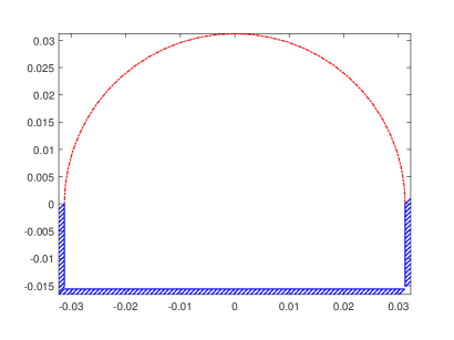
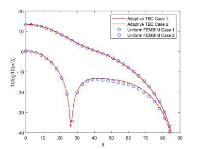
Figure 2. Example 1: (left) Geometry of the cavity; (right) Backscatter RCS for both cases by using the adaptive finite element DtN method (Adaptive TBC) and the coupling of finite element method and boundary integral method (FEMBIM).

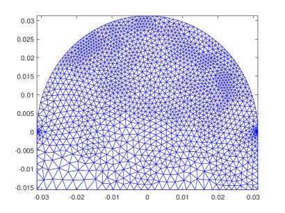
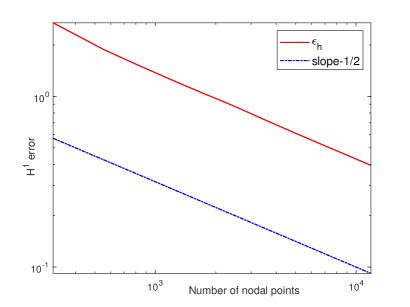
Figure 3. Example 1: (left) Adaptive mesh after 4 iterations with a total number of nodal points $1674$; (right) Quasi-optimality of the a posteriori error estimates.

Table 2. Example 1: comparison of numerical results using the adaptive meshe and uniform mesh refinements. ${\rm DoF}_{h}$ is the degree of freedom or the number of nodal points for the mesh $\mathcal{M}_{h}$.

Adaptive Mesh		Uniform Mesh
${\rm DoF}_{h}$	RCS	${\rm DoF}_{h}$	RCS
310	0.0061367	310	0.0061367
509	0.0042423
1173	0.0029691	1199	0.0032574
2298	0.0023687
4438	0.0021304	4648	0.0022952
10293	0.0018429
17875	0.0017774	18146	0.0018434
23463	0.0017182
39878	0.0016583	40234	0.0017165
65544	0.0016212
104706	0.0015878	111274	0.0016248

7.2. Example 2

This example also concerns the TM polarization. We compute the backscatter RCS for a coated rectangular cavity, which has a width $1.2\lambda$ and a depth $0.8\lambda$. The each vertical side of the cavity wall is coated with a thin layer of some absorbing material, as seen in Figure 4. The thickness of the coating is $0.012\lambda$ for both sides. The coating is made of a homogeneous absorbing medium, which has a relative permittivity $\epsilon_{\rm r}=12+0.144{\rm i}$ and a relative permeability $\mu_{r}=1.74+3.306{\rm i}$. This is a multi-scale problem and it is very difficult to compute the numerical solution by using the finit element with uniform mesh refinements in order to resolve the thin absorbing layers. Figure 4 plots the backscatter RCS. Again, the solid line is the result by using the adaptive finite element DtN method, while the circles stand for the result by using the coupling of the finite element method and the boundary integral method (FEMBIM). We take the same stopping strategy as the one for Example 1: the adaptive finite element DtN method is stopped when the number of nodal points is over 15000. For the FEMBIM, the result is computed by using a uniform mesh with the number of nodal points $112059$. Using a representative example of incident angle $\theta=\pi/3$, we present the refined mesh after 2 iterations with 1508 ${\rm DoF}_{h}$ and the a posteriori error estimates in Figure 5. It is clear to note that the method can capture the behavior of the numerical solution in the two thin absorbing layers and displays the quasi-optimality between the meshes and the associated numerical complexity, i.e., $\varepsilon_{h}=O({\rm DoF}_{h}^{-1/2})$ holds asymptotically. As a comparison, we show the backscatter RCS by using the finite element DtN method with the adaptive mesh and uniform mesh refinements in Table 3. Apparently, the adaptive mesh refinements yields a better numerical performance than the uniform mesh refinements does, since the former can give more accurate results even by using fewer number of nodal points.

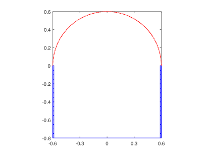
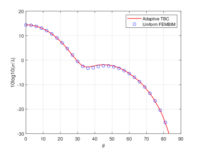
Figure 4. Example 2: (left) Geometry of the cavity with thin absorbing layers on the two vertical sides; (right) Backscatter RCS by using the adaptive finite element DtN method (Adaptive TBC) and the coupling of finite element method and boundary integral method (FEMBIM).

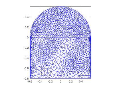
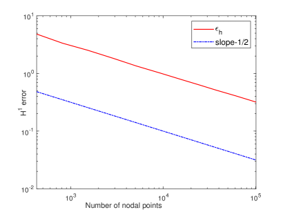
Figure 5. Example 2: (left) Adaptive mesh after 2 iterations with a total number of nodal points $1508$; (right) Quasi-optimality of the a posteriori error estimates.

Table 3. Example 2: comparison of numerical results using the adaptive meshe and uniform mesh refinements. ${\rm DoF}_{h}$ is the degree of freedom or the number of nodal points for the mesh $\mathcal{M}_{h}$.

Adaptive mesh		Uniform mesh
${\rm DoF}_{h}$	RCS	${\rm DoF}_{h}$	RCS
429	0.84613846	429	0.8461385
818	0.54563374
1518	0.61134157
2924	0.55103383	3563	0.6429673
5118	0.57427862
9358	0.57726558
15928	0.58262461	13876	0.6048405
24786	0.58383447
37473	0.57827731	30981	0.5982348
61332	0.57586437	55028	0.5967787
100740	0.57570343	124138	0.5925520
161478	0.57704918	277710	0.5908951

7.3. Example 3

In the above two examples, the rectangle-shaped cavities are below the ground. For such cavities, we may either use the coupling of the finite element method and boundary integral method (FEMBIM) method [24] or the finite element perfectly matched layer (FEPML) method [33] to solve the scattering problems. In this example, we consider the TM case but the structure of the cavity is above the ground. The width and depth of the cavity is $1.2\lambda$ and $0.8\lambda$, respectively. However, we set two thin rectangular PEC humps in the middle of the cavity with height $\frac{16}{15}\lambda$ and $\frac{8}{15}\lambda$, respectively. The width is $\frac{1}{20}\lambda$ for both humps. The geometry of the cavity and the backscatter RCS are shown in Figure 6. Again, the stopping criterion is that the mesh refinement is stopped when the number of nodal points is over 15000. Using the incident angle $\theta=\pi/3$ as an example, we show the refined mesh after two iterations with the number of nodal points $1409$ and the a posteriori error estimates in Figure 7. The adaptive DtN method is able to generate locally refined meshes around the corners of the cavity where the solution has a singularity. The quasi-optimality is also obtained for the a posteriori error estimates.

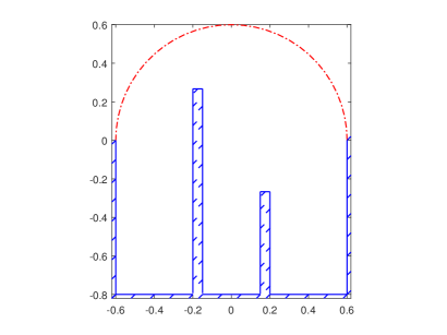
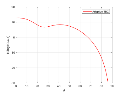
Figure 6. Example 3: (left) Geometry of the cavity; (right) Backscatter RCS by using the adaptive finite element DtN method.

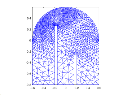
Figure 7. Example 3: (left) Adaptive mesh after 2 iterations with a total number of nodal points $1409$; (right) Quasi-optimality of the a posteriori error estimates.

7.4. Example 4

In this example, we consider the cavity scattering problem for TE polarization. The cavity is a rectangle with a fixed width $0.025\rm m$ and a fixed depth $0.015\rm m$. The cavity is empty and filled with the same homogeneous medium as that in the free space. Instead of considering the illumination by a plane wave with a fixed frequency, we compute backscatter RCS with the frequency ranging from $2\,\rm GHz$ to $18\,\rm GHz$. Correspondingly, the range of the aperture of cavity is from $\frac{1}{6}\lambda$ to $1.5\lambda$. The incident angle is $\frac{4}{9}\pi$. Figure 8 shows the backward RCS by using the adaptive finite element DtN method, where the red-solid line and blue circles show the results obtained by applying (6.4) and (6.2), respectively. The stopping criterion is that the mesh refinement is stopped when the number of nodal points is over 25000.

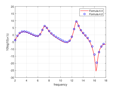
Figure 8. Example 4: Backscatter RCS.

8. Conclusion

In this paper, we have developed an adaptive finite element DtN method for solving the open cavity scattering problems. The a posteriori error estimates are obtained for both of the TM and TE polarization waves. The estimates consist of the finite element discretization error and the DtN operator truncation error. The latter is shown to decay exponentially with respect to the truncation number. Along the line of this research, future work includes extending the analysis to the more challenging three-dimensional problem, where Maxwell’s equations need to be considered, and the problems of elastic wave scattering from cavities. An open problem is to develop a DtN based TBC on the upper semi-circle enclosing the cavities. We hope to report the progress on these aspects elsewhere in the future.

References

- [1] H. Ammari, G. Bao, and A. Wood, An integral equation method for the electromagnetic scattering from cavities, Math. Meth. Appl. Sci., 23 (2000), 1057–1072.
- [2] H. Ammari, G. Bao, and A. Wood, Analysis of the electromagnetic scattering from a cavity, Jpn. J. Indus. Appl. Math., 19 (2001), 301–308.
- [3] H. Ammari, G. Bao, and A. Wood, A cavity problem for Maxwell’s equations, Meth. Appl. Anal., 9 (2002), 249–260.
- [4] I. Babuška and A. Aziz, Survey lectures on mathematical foundation of the finite element method, in the Mathematical Foundations of the Finite Element Method with Application to the Partial Differential Equations, ed. by A.Aziz, Academic Press, New York, 1973, 5–359.
- [5] G. Bao, J. Gao, and P. Li, Analysis of direct and inverse cavity scattering problems, Numer. Math. Theor. Meth. Appl., 4 (2011), 335–358.
- [6] G. Bao, J. Gao, J. Lin, and W. Zhang, Mode matching for the electromagnetic scattering from three dimensional large cavities, IEEE Trans. Antennas Propag., 60 (2012), 1–7.
- [7] G. Bao, G. Hu, and T. Yin, Time-harmonic acoustic scattering from locally perturbed half-planes, SIAM J. Appl. Math., 78 (2018), 2672–2691.
- [8] G. Bao and W. Sun, A fast algorithm for the electromagnetic scattering from a large cavity, SIAM J. Sci. Comput., 27 (2005), 553–574.
- [9] G. Bao and K. Yun, Stability for the electromagnetic scattering from large cavities, Arch. Ration. Mech. Anal., 3 (2016), 1003–1044.
- [10] G. Bao, K. Yun, and Z. Zhou, Stability of the scattering from a large electromagnetic cavity in two dimensions, SIAM J. Math. Anal., 44 (2012), 383–404.
- [11] G. Bao and W. Zhang, An improved mode matching method for large cavities, IEEE Antennas Wireless Propag. Lett., 4 (2005), 393–396.
- [12] M. Durán, I. Muga, and J.-C. Nédélec, The Helmholtz equation in a locally perturbed half-space with non-absorbing boundary, Arch. Ration. Mech. Anal., 191 (2009), 143–172.
- [13] F. Hecht, New development in FreeFem++, J. Numer. Math., 20 (2012), 251–265.
- [14] J. Huang and A. Wood, Numerical simulation of electromagnetic scattering induced by an overfilled cavity in the ground plane, IEEE Antennas Wireless Propag. Lett., 4 (2005), 224–228.
- [15] J. Huang, A. Wood, and M. Havrilla, A hybrid finite element-laplace transform method for the analysis of transient electromagnetic scattering by an over-filled cavity in the ground plane, Commun. Comput. Phys., 5 (2009), 126–141.
- [16] X. Jiang, P. Li, and W. Zheng, Numerical solution of acoustic scattering by an adaptive DtN finite element method, Commun. Comput. Phys., 13 (2013), 1227–1244.
- [17] X. Jiang, P. Li, J. Lv, and W. Zheng, An adaptive finite element method for the wave scattering with transparent boundary condition, J. Sci. Comput., 72 (2017), 936–956.
- [18] X. Jiang, P. Li, J. Lv, Z. Wang, H. Wu and W. Zheng, An adaptive finite element DtN method for Maxwell’s equation in biperiodic structures, arXiv:1811.12449.
- [19] J.-M. Jin, Electromagnetic scattering from large, deep, and arbitrarily- shaped open cavities, Electromagn., 1 (1998), 3–34.
- [20] J.-M. Jin, The Finite Element Method in Electromagnetics , Wiley & Son, New York, 2002.
- [21] J.-M. Jin and J. L. Volakis, A hybrid finite element method for scattering and radiation by micro strip patch antennas and arrays residing in a cavity, IEEE Trans. Antennas Propag., 39 (1991), 1598–1604.
- [22] H. Li, H. Ma, and W. Sun, Legendre spectral Galerkin method for electromagnetic scattering from large cavities, SIAM J. Numer. Anal., 51 (2013), 253–276.
- [23] P. Li, A survey of open cavity scattering problems, J. Comp. Math., 36 (2018), 1–16.
- [24] P. Li and A. Wood, A two-dimensional Helmholtz equation solution for the multiple cavity scattering problem, J. Comput. Phys., 240 (2013), 100–120.
- [25] P. Li, H. Wu, and W. Zheng, An overfilled cavity problem for Maxwell’s equations, Math. Meth. Appl. Sci., 15 (2012), 1951–1979.
- [26] P. Li and X. Yuan, Convergence of an adaptive finite element DtN method for the elastic wave scattering by periodic structures, Comput. Methods Appl. Mech. Engrg., 360 (2020), 112722.
- [27] J. Liu and J.-M. Jin, A special higher order finite-element method for scattering by deep cavities, IEEE Trans. Antennas Propag., 5 (2000), 694–703.
- [28] A. H. Schatz, An observation concerning Ritz–Galerkin methods with indefinite bilinear forms, Math. Comp., 28 (1974), 959–962.
- [29] A. Wood, Analysis of electromagnetic scattering from an overfilled cavity in the ground plane, J. Comput. Phys., 215(2006), 630–641.
- [30] Y. Wang, K. Du, and W. Sun, A second-order method for the electromagnetic scattering from a large cavity, Numer. Math. Theor. Meth. Appl., 1 (2008), 357–382.
- [31] Z. Wang, G. Bao, J. Li, P. Li, and H. Wu, An adaptive finite element method for the diffraction grating problem with transparent boundary condition, SIAM. J. Numer. Anal., 3 (2015), 1585-1607.
- [32] G. N. Watson, A Treatise on the Theory of Bessel Functions, Cambridge University Press, Cambridge, UK, 1922.
- [33] X. Wu and W. Zheng, An adaptive perfectly matched layer method for multiple cavity scattering problems, Commun. Comput. Phys., 19 (2016), 534–558.
- [34] D. Zhang, F. Ma, and H. Dong, A finite element method with rectangular perfectly matched layers for the scattering from cavities, J. Comput. Math., 27 (2009), 812–834.