Theoretical and numerical comparison of the Karush-Kuhn-Tucker
and value function reformulations in bilevel optimization

Abstract.

The Karush-Kuhn-Tucker and value function (lower-level value function, to be precise) reformulations are the most common single-level transformations of the bilevel optimization problem. So far, these reformulations have either been studied independently or as a joint optimization problem in an attempt to take advantage of the best properties from each model. To the best of our knowledge, these reformulations have not yet been compared in the existing literature. This paper is a first attempt towards establishing whether one of these reformulations is best at solving a given class of the optimistic bilevel optimization problem. We design a comparison framework, which seems fair, considering the theoretical properties of these reformulations. This work reveals that although none of the models seems to particularly dominate the other from the theoretical point of view, the value function reformulation seems to numerically outperform the Karush-Kuhn-Tucker reformulation on a Newton-type algorithm. The computational experiments here are mostly based on test problems from the Bilevel Optimization LIBrary (BOLIB).

1. Introduction

Our focus in this paper is the standard optimistic bilevel optimization problem

$$\underset{x,y}{\min}\leavevmode\nobreak\ F(x,y)\;\;\mbox{s.t.}\;\;G(x,y)\leq 0,\;\,y\in S(x),$$ (P)

also known as the upper-level problem. The functions $F:\mathbb{R}^{n}\times\mathbb{R}^{m}\to\mathbb{R}$ and $G:\mathbb{R}^{n}\times\mathbb{R}^{m}\to\mathbb{R}^{p}$ represent the upper-level objective and upper-level constraint functions, respectively, while $x\in\mathbb{R}^{n}$ (resp. $y\in\mathbb{R}^{m}$) corresponds to the upper-level (resp. lower-level) variable. Note that we have $n,m,p\in{{\mathbb{N}^{*}:=\{1,\,2,\ldots\}}}$. In the sequel, we collect all the feasible upper-level variables as follows:

$$X:=\left\{x\in\mathbb{R}^{n}|\;\exists y\in\mathbb{R}^{m}:\;\,G(x,y)\leq 0\right\}.$$ (1.1)

In problem (P), the set-valued mapping $S:\mathbb{R}^{n}\rightrightarrows\mathbb{R}^{m}$ describes the set of optimal solutions of the following parametric optimization problem, known as the lower-level problem:

$$\underset{y}{\min}\leavevmode\nobreak\ \left\{f(x,y)\mid g(x,y)\leq 0\right\}.$$ (1.2)

That is, precisely, we have

$$S(x):=\left\{\begin{array}[]{lll}\arg\underset{y}{\min}\leavevmode\nobreak\ \left\{f(x,y)\mid g(x,y)\leq 0\right\}&\mbox{if}&x\in X,\\ \emptyset&\mbox{if}&x\in\mathbb{R}^{n}\setminus X.\end{array}\right.$$ (1.3)

The functions $f:\mathbb{R}^{n}\times\mathbb{R}^{m}\to\mathbb{R}$ and $g:\mathbb{R}^{n}\times\mathbb{R}^{m}\to\mathbb{R}^{q}$ (with $q\in\mathbb{N}^{*}$) correspond to the lower-level objective and lower-level constraint functions, respectively.

Throughout this paper, the upper- and lower-level problems are constrained only by inequality constraints, for the sake of simplicity. However, all the analysis conducted here remains valid (of course with the corresponding adjustments) if equality constraints are added to the upper-level and/or lower-level feasible set of problem (P). Furthermore, to focus our attention only on the main points, we assume throughout the paper that $S(x)\neq\emptyset$ for all $x\in X$.

In the pursue of tractable approaches to solve (P) from the perspective of standard constrained optimization, two main approaches have been considered to reformulate the problem as a single-level optimization problem. Considering the Lagrangian function

$$\ell(x,y,z):=f(x,y)+z^{\top}g(x,y),$$ (1.4)

of problem (1.2) and assuming that $f$ and $g$ are differentiable w.r.t. $y$, the first one-level reformulation of problem (P) is the Karush-Kuhn-Tucker (KKT) reformulation that can be written as

$$\begin{array}[]{rl}\underset{x,\,y,\,z}{\min}&F(x,y)\\ \,\mbox{ s.t. }&G(x,y)\leq 0,\ \ \nabla_{2}\ell(x,y,z)=0,\\ &\,\,g(x,y)\leq 0,\ \ z\geq 0,\ \ z^{\top}g(x,y)=0,\end{array}$$ (KKTR)

where $\nabla_{2}\ell$ corresponds to the gradient of $\ell$ w.r.t. $y$. The second main approach to transform (P) into a single-level optimization problem is the lower-level value function (LLVF) reformulation

$$\begin{array}[]{lll}&\underset{x,\,y}{\min}&F(x,y)\\ &\mbox{ s.t. }&G(x,y)\leq 0,\ \ g(x,y)\leq 0,\ \ f(x,y)-\varphi(x)\leq 0,\end{array}$$ (LLVFR)

where $\varphi$ denotes the optimal value function of the lower-level problem:

$$\varphi(x):=\underset{y}{\min}\leavevmode\nobreak\ \left\{f(x,y)\mid g(x,y)\leq 0\right\}.$$ (1.5)

Both problems (KKTR) and (LLVFR) have been independently studied in various papers. For example, [7] provides a detailed analysis of the relationship between (KKTR) and the original problem (P). Solution algorithms specifically tailored to reformulation (KKTR) can be found in [2, 6, 11, 29], for example. As for (LLVFR), most of the work so far has been dedicated to the development of optimality conditions (see, e.g., [8, 13, 28, 43]), but a few works on numerical methods have appeared recently. Namely, the papers [25, 39, 40] propose methods for nonlinear bilevel optimization based on (LLVFR); algorithms in [10, 9] suggest techniques to solve special cases of problem (LLVFR), where relaxation schemes are used to deal with the value function (1.5); the authors of [23, 24] proposed numerical methods to solve special bilevel programs by exploiting a connection between problem (LLVFR) and a generalized Nash equilibrium problem. A semismooth Newton-type method for (LLVFR) is developed in [16]. A few papers (see, e.g., [40, 42]) have also proposed methods based on a combination of (KKTR) and (LLVFR), in order to take advantage of some interesting features from each of these reformulations.

Note however that problems (KKTR) and (LLVFR) taken separately, are reformulations of the same problem (P), but which by their nature, seem to be far apart from each other. It therefore seems interesting to find a way to compare them. This paper is a first attempt towards establishing whether one of these reformulations is best at solving a given class of problem (P). Our framework for comparing problems (KKTR) and (LLVFR) revolves around the 5 questions below, which gradually go from the basic considerations often taken into account when solving an optimization problem to a numerical performance from the perspective of a certain numerical method:

(Q1) How are problems (KKTR) and (LLVFR) related to problem (P) and how do the requirements for these problems to be smooth or locally Lischitz continuous optimization problems compare to each other? This question is considered in Subsection 2.1, where first of all, we discuss the challenges in solving (P) via (KKTR) or (LLVFR) and highlight the fact that despite the apparent strong conditions needed to ensure a close link between the former problem and (P), aiming to solve (LLVFR) as a smooth ($\mathcal{C}^{1}$) optimization problem requires even much stronger conditions.

(Q2) How do the qualification conditions needed to derive necessary optimality conditions for (KKTR) and (LLVFR) relate to each other? The analysis of this question conducted in Subsection 3.1 shows that on top of the aforementioned technical requirements to establish (LLVFR) as a smooth or local Lipschitz optimization problem, the model does not seem to provide the same level of flexibility for the fulfilment of qualification conditions that (KKTR) enjoys thanks to its connection to mathematical programs with equilibrium constraints (MPCCs).

(Q3) How do the optimality conditions resulting from (KKTR) and (LLVFR) compare to each other? Acknowledging the fact that each of these reformulations can lead to a wide variety of optimality concepts, we identify specific classes of conditions and problems that enable sensible relationships between the two models and subsequently to tractable solution algorithms; see Subsection 3.2 for details on the optimality conditions and Section 4 for the algorithms.

(Q4) How do the qualification conditions necessary to establish the convergence results for a corresponding version of the semismooth Newton method compare to each other? As the standard framework to analyse and solve (LLVFR) is via the partial exact penalization [43], considering a similar approach for (KKTR) seems to be the most sensible methodological approach to compare our reformulations. Hence, as a by-product of this paper, we develop, probably for the first time, a semismooth Newton-type algorithm for (KKTR) and compare it to the corresponding algorithm for (LLVFR) developed in [16]. As expected, (KKTR) appears to be more demanding, in terms of the derivative requirement for the lower-level problem (3rd order derivatives are necessary for convergence analysis and implementation). However, from a theoretical point of view, there does seem to be a clear dominance of the qualification conditions for convergence of the method of one model on the other one; cf. Section 4.

(Q5) Which one from problems (KKTR) and (LLVFR) leads to a more efficient algorithm, in terms of number of iterations, computing time, numerical accuracy, and rate of convergence? Our computational experiments, based on various test problems, including those from the BOLIB Library [46], show that our semismooth Newton method for (LLVFR) generally outperforms the one based on the (KKTR) model, for all the aforementioned performance measures. One of the surprising observation from the numerical computation is that the superiority of (LLVFR) remains for all the aforementioned measures, even for problem classes where 3rd order derivatives for lower-level problems are non-zero, despite the expectation that in this case, better approximations of the curvature of the lower-level optimal solution set could potentially reduce the number of iterations.

Overall, as it will be clear from the analysis in the remaining sections, the main take away of this paper is that from the theoretical point of view, it is not possible to claim that one of the reformulations is better than the other, although (KKTR) seems to provide a framework for more tractable qualification conditions for optimality conditions an convergence analysis, thanks to its relationship to MPCCs. However, from the numerical perspective, the framework and test problems considered in this paper suggest that problem (LLVFR) is a much better option.

After addressing (Q1) in Subsection 2.1, the general framework for the analysis of the other questions is introduced in Subsection 2.2. Questions (Q2), (Q3), (Q4), and (Q5) are then addressed, in this order, in the subsequent parts of the paper.

2. Links to the original problem and framework for comparison

To start this section, we introduce some notation that will be used throughout the paper. Namely, we associate a number of index sets to the inequality constraints involved in problems (KKTR) and (LLVFR). For instance, for a point $(\bar{x},\bar{y})$ in the upper-level feasible set of problem (P), we denote the indices of the constraints active at this point by

$$I^{1}:=I^{G}(\bar{x},\bar{y}):=\left\{i\leavevmode\nobreak\ |\;\,G_{i}(\bar{x},\bar{y})=0\right\}.$$ (2.1)

Since part of the analysis to be conducted in this paper will be based on the stationary points of each of the reformulations above, we associate to a point $(\bar{x},\bar{y})$ in the upper-level feasible set, a Lagrange multiplier $\bar{u}$. Then, considering the fact that the optimality conditions for problem (KKTR) or (LLVFR) will lead to the complementarity system $\bar{u}\geq 0$, $G(\bar{x},\bar{y})\leq 0$, $\bar{u}^{\top}G(\bar{x},\bar{y})=0$, we partition the corresponding indices in the following standard way:

$$\begin{array}[]{l}\eta^{1}:=\eta^{G}(\bar{x},\bar{y},\bar{u}):=\{i\leavevmode\nobreak\ |\;\,\bar{u}_{i}=0,\;\,G_{i}(\bar{x},\bar{y})<0\},\\ \theta^{1}:=\theta^{G}(\bar{x},\bar{y},\bar{u}):=\{i\leavevmode\nobreak\ |\;\,\bar{u}_{i}=0,\;\,G_{i}(\bar{x},\bar{y})=0\},\\ \nu^{1}:=\nu^{G}(\bar{x},\bar{y},\bar{u}):=\{i\leavevmode\nobreak\ |\;\,\bar{u}_{i}>0,\;\,G_{i}(\bar{x},\bar{y})=0\}.\end{array}$$ (2.2)

Similarly, considering the constraint $g(x,y)\leq 0$ appearing in (KKTR) and (LLVFR), as well as $z\geq 0$ in (KKTR), the corresponding index sets at $(\bar{x},\bar{y})$ (resp. $(\bar{x},\bar{y},\bar{v})$), $\bar{z}$ (resp. $(\bar{z},\bar{w})$), and $(\bar{x},\bar{z})$ (resp. $(\bar{x},\bar{z},\bar{w})$), where $\bar{v}$, $\bar{w}$, and $\bar{w}$ represent the Lagrange multipliers, are respectively defined as

$$\begin{array}[]{llll}I^{2}:=I^{g}(\bar{x},\bar{y}),&\eta^{2}:=\eta^{g}(\bar{x},\bar{y},\bar{v}),&\theta^{2}:=\theta^{g}(\bar{x},\bar{y},\bar{v}),&\nu^{2}:=\nu^{g}(\bar{x},\bar{y},\bar{v}),\\ I^{3}:=I^{z}(\bar{z}),&\eta^{3}:=\eta^{z}(\bar{z},\bar{w}),&\theta^{3}:=\theta^{z}(\bar{z},\bar{w}),&\nu^{3}:=\nu^{z}(\bar{z},\bar{w}),\\ I^{4}:=I^{g}(\bar{x},\bar{z}),&\eta^{4}:=\eta^{g}(\bar{x},\bar{z},\bar{w}),&\theta^{4}:=\theta^{g}(\bar{x},\bar{z},\bar{w}),&\nu^{4}:=\nu^{g}(\bar{x},\bar{z},\bar{w})\end{array}$$ (2.3)

with the first and second lines here being associated to (KKTR) and the last one related to problem (LLVFR). For vectors $d^{i}\in\mathbb{R}^{n}$, $d^{j}\in\mathbb{R}^{m}$, and $d^{k}\in\mathbb{R}^{p}$, for example, with $i,j,k\in\mathbb{N}$, $d^{ij}$ and $d^{ijk}$ represent the combined vectors

$$d^{ij}:=\left[\begin{array}[]{c}d^{i}\\ d^{j}\end{array}\right]\;\;\mbox{ and }\;\;d^{ijk}:=\left[\begin{array}[]{c}d^{i}\\ d^{j}\\ d^{k}\end{array}\right],$$

respectively. For a function $\psi:\mathbb{R}^{\tilde{n}}\times\mathbb{R}^{\tilde{m}}\times\mathbb{R}^{\tilde{p}}\rightarrow\mathbb{R}^{\tilde{q}}$, $\nabla_{i}\psi(a,b,c)$ with $i\in\{1,2,3\}$, corresponds to the gradient of $\psi$ w.r.t. the $i$th variable $a$, $b$ or $c$. Furthermore, unless otherwise stated, $\nabla_{i,j}\psi(a,b,c)$ (resp. $\nabla^{2}_{ij}\psi(a,b,c)$) with $i,j\in\{1,2,3\}$, denotes the gradient (resp. second order derivative) of $\psi$ w.r.t. the $i$th and $j$th variables. Note that in the sequel, the corresponding versions of the function $\psi$ could have 2, 3, 4 or more variables. In those cases, the same logic presented here will be used.

2.1. Nature of reformulations and relationships to original problem

We start this subsection by looking at the relationships between (P) and its reformulations (KKTR) and (LLVFR). For the link between (KKTR) and (P), we need two properties; i.e., convexity and a lower-level regularity condition. These assumptions are needed to help ensure that inclusion $y\in S(x)$ can be written in terms of the KKT conditions present in the feasible set of problem (KKTR).

Definition 2.1 (lower-level convexity).

The lower-level optimization problem (1.2) is said to be convex if the functions $f(x,.)$ and $g_{i}(x,.)$, $i=1,\ldots,q$ are convex for all $x\in X$. The problem will be said to be fully convex if the latter functions are convex w.r.t. $(x,y)$.

For the lower-level regularity, we use the standard lower-level Mangasarian-Fromowitz constraint qualification (LMFCQ), which holds at $(\bar{x},\bar{y})$ if there exits $d$ such that

$$\nabla_{2}g_{i}(\bar{x},\bar{y})^{\top}d<0\;\,\mbox{ for all }\;\,i\in I^{2}.$$ (2.4)

For a point $(x,y)$ such that $G(x,y)\leq 0$ and $(x,y)\in\text{gph}\,S$, it is well-known that if the LMFCQ holds at $(x,y)$, then the following set of lower-level Lagrange multipliers is non-empty:

$$\Lambda(x,y):=\left\{\left.z\in\mathbb{R}^{q}\right|\;\,\nabla_{2}\ell(x,y,z)=0,\;\,z\geq 0,\;\,g(x,y)\leq 0,\;\,z^{\top}g(x,y)=0\right\}.$$ (2.5)

We have the following result established in [7].

Theorem 2.2 (local and global relationship between (KKTR) and (P)).

Let $G$ be independent from $y$ and $f(x,.)$ and $g_{i}(x,.)$, $i=1,\ldots,q$ be convex and $\mathcal{C}^{1}$ for all $x\in X$. Then, the following statements hold:

• Let $(\bar{x},\bar{y})$ be globally (resp. locally) optimal for (P) and the LMFCQ be satisfied at $(\bar{x},y)$, $y\in S(\bar{x})$. Then, for each $z\in\Lambda(\bar{x},\bar{y})$, the point $(\bar{x},\bar{y},z)$ is a global (resp. local) optimal solution of (KKTR).

• Let the LMFCQ hold at all $(x,y)$, $y\in S(x)$, $x\in X$ (resp. at $(\bar{x},y)$, $y\in S(\bar{x})$) and $(\bar{x},\bar{y},z)$ be a global (resp. local) optimal solution (resp. for all $z\in\Lambda(\bar{x},\bar{y})$) of (KKTR), then the point $(\bar{x},\bar{y})$ is a global (resp. local) optimal solution of problem (P).

It is shown in [7] that this result is very sensitive to convexity and the constraint qualification, as it typically fails if one of these assumptions does not hold. More details on the results can be found in that paper; some of the key issues faced when attempting to solve (P) via (KKTR) can be found in the next examples below. Before that, we state the equivalence between (P) and (LLVFR), which is valid locally and globally without any assumption (apart from requiring that $\mbox{gph}S\neq\emptyset$, assumed to be valid throughout the paper as stated in the introduction), given that the lower-level optimal solution set-valued mapping $S$ (1.3) can be equivalently written as

$$S(x):=\left\{y\in\mathbb{R}^{m}\,|\;g(x,y)\leq 0,\;\;f(x,y)-\varphi(x)\leq 0\right\}\;\;\mbox{ for all }\;\,x\in X.$$

Theorem 2.3 (local and global relationship between (LLVF) and (P)).

$(\bar{x},\bar{y})$ is a local (resp. global) optimal solution of (LLVFR) if and only if the point is a local (resp. global) optimal solution of (P).

Example 2.1 (problem (LLVFR) has an optimal solution but (KKTR) does not have one).

Consider an example of problem (P) from [7] with the corresponding functions defined by

$$F(x,y):=x,\;\,G(x,y):=-x,\;\,f(x,y):=y_{1},\;\,\mbox{ and }\;\,g(x,y):=\left(y^{2}_{1}-y_{2}-x,\;y^{2}_{1}+y_{2}\right)^{\top}.$$

For this example, it is shown in [7] that $(\bar{x},\bar{y})=(0,0)$ is the global optimal solution of (P) and hence of problem (LLVFR) (cf. Theorem 2.3), but (KKTR) does not have any solution.

Example 2.2 (problems (LLVFR) and (KKTR) both have optimal solutions, but which are completely different from each other).

Consider an example of problem (P) from [7] with the corresponding functions defined by

$$F(x,y):=(x-1)^{2}+y^{2},\;\;f(x,y):=x^{2}y,\;\mbox{ and }\;g(x,y):=y^{2}.$$ (2.6)

The global optimal solution of the corresponding problem (P) is $(\bar{x},\bar{y})=(1,0)$. The feasible sets of (KKTR) and (LLVFR) can be respectively obtained as

$$S_{1}=\left\{\left.(x,y,z)\right|z\in\mathbb{R}_{+},\;\,x=y=0\right\}\;\mbox{ and }\;S_{2}=\left\{\left.(x,y)\right|\leavevmode\nobreak\ x\in\mathbb{R},\;\,y=0\right\}.$$

Obviously, $(1,0)$ is also the optimal solution of (LLVFR). However, the global optimal solution of (KKTR) is $(0,0,z)$ for any $z\geq 0$. It is pointed out in [7] that this is due to the failure of the lower-level regularity condition; cf. Theorem 2.2. This clearly shows that the optimal solution of problem (KKTR) need not be optimal for (P), while this cannot be the case for (LLVFR); cf. Theorem 2.3.

Example 2.3 (problems (LLVFR) and (KKTR) both have optimal solutions which are equivalent in the sense of Theorem 2.2).

Here, we consider a variant of the problem described in (2.6); i.e.,

$$F(x,y):=(x-1)^{2}+y^{2},\;\;f(x,y):=x^{2}y,\;\mbox{ and }\;g(x,y):=y^{2}-1,$$ (2.7)

where the lower-level constraint function is slightly modified. The lower-level problem is convex and the LMFCQ holds at any lower-level feasible point. The points $(\bar{x},\bar{y})=(1,-1)$ and $(\bar{x},\bar{y})=(0,0)$ are global optimal solutions of the version of (P) defined in (2.7) and hence of the corresponding (LLVFR). The feasible sets of (KKTR) and (LLVFR) in the context of (2.7) are respectively given by

$$S_{1}=\left\{\left.(x,y,z)\right|\leavevmode\nobreak\ \left(x=z=0,\,y^{2}\leq 1\right)\leavevmode\nobreak\ {\rm or}\leavevmode\nobreak\ \left(x^{2}=2z\leavevmode\nobreak\ \geq 0,\,y=-1\right)\right\}\,\mbox{ and }\,S_{2}=\left\{\left.(x,y)\right|\leavevmode\nobreak\ x^{2}y+x^{2}=0,\,y^{2}\leq 1\right\}.$$

Clearly, both $(\bar{x},\bar{y},\bar{z})=(1,-1,0.5)$ and $(\bar{x},\bar{y},\bar{z})=(0,0,0)$ are optimal solutions of (KKTR). The feasible sets in Figure 1 clearly exhibit the differences between the sizes of problems (KKTR) and (LLVFR); the former has more variables and constraints than the latter. Table 1, provided later in this section, contains more general details on the dimensions of the problems.

Figure 1. Feasible sets to (KKTR) and (LLVFR). The red lines represent the feasible sets and green points stand for the global optimal solutions.

Now, we go beyond the relationship analysis above and start to consider the question of how to solve problems (KKTR) and (LLVFR) and how the processes of getting to a solvable model compare to each other. To design a solution algorithm for an optimization problem, the nature of the functions involved is critical in choosing the most suitable approach. For instance, we would like to look at the framework, based on problem (P) data, ensuring that the reformulations under consideration are smooth ($\mathcal{C}^{1}$) or Lipschitz continuous optimization problems. Obviously, (KKTR) is a smooth optimization problem if the following conditions are satisfied:

$$\left\{\begin{array}[]{l}F\;\mbox{ and }\;G\;\mbox{ are }\;\mathcal{C}^{1};\\ f(x,.)\;\mbox{ and }\;g(x,.)\;\mbox{ are }\;\mathcal{C}^{1}\;\mbox{ for all }x\in\mathbb{R}^{n};\\ \nabla_{2}f\;\mbox{ and }\;\nabla_{2}g\;\mbox{ are }\;\mathcal{C}^{1}\;\mbox{ in }(x,y).\end{array}\right.$$ (2.8)

On the other hand, to ensure that (LLVFR) is smooth, the following conditions need to hold:

$$\begin{array}[]{l}F,\;G,\;f,\;g,\;\mbox{ and }\;\varphi\;\mbox{ are }\;\mathcal{C}^{1}.\end{array}$$ (2.9)

Unfortunately, it is quite demanding to ensure that $\varphi$ is a smooth function. To guaranty that this is the case, we present the following result due to Fiacco [14].

For this result, we need another, much stronger, lower-level regularity condition. Namely, the lower-level linear independence constraint qualification (LLICQ) that will be said to hold at $(\bar{x},\bar{y})$ if the following family of gradients is linearly independent:

$$\left\{\left.\nabla_{2}g_{i}(\bar{x},\bar{y})\,\right|\;i\in I^{2}\right\}.$$ (2.10)

It is well-known that under this condition, the set of lower-level Lagrange multipliers (2.5) is single-valued at the point $(\bar{x},\bar{y})$. Furthermore, considering $(\bar{x},\bar{z},\bar{v})$ such that $\bar{v}\in\Lambda(\bar{x},\bar{z})\neq\emptyset$, the lower-level strict complementarity condition (LSCC) will be said to hold at this point if

$$\theta^{g}(\bar{x},\bar{y},\bar{v})=\emptyset.$$ (2.11)

Theorem 2.4 (continuous differentiability of $\varphi$).

Let the functions $f$ and $g$ be $\mathcal{C}^{2}$. Suppose that the LLICQ and holds at $(\bar{x},\bar{y})$ and the lower-level second order sufficient condition (LSOSC)

$$d^{\top}\nabla_{22}^{2}\ell(\bar{x},\bar{y},\bar{v})d>0,\;\,\forall d\neq 0\;\,\mbox{ s.t. }\;\,\nabla_{2}f(\bar{x},\bar{y})^{\top}d=0,\;\,\nabla_{2}g_{i}(\bar{x},\bar{y})^{\top}d\leq 0\;\mbox{ for }\;i\in I^{2},$$ (2.12)

with $\Lambda(\bar{x},\bar{y})=\left\{\bar{v}\right\}$, holds. Furthermore, if the LSCC holds at $(\bar{x},\bar{y},\bar{v})$, then, the function $\varphi$ is continuously differentiable around the point $\bar{x}$.

Obviously, these conditions are far much stronger than the ones needed for the KKT reformulation (KKTR). Moreover, even if one adds the assumptions of Theorem 2.2 to (2.8), the framework for (LLVFR) to be smooth is still far more demanding than the one necessary for building (KKTR) and ensuring that it is a smooth optimization problem. Furthermore, it is important to observe that the assumptions in Theorem 2.4 ensure the differentiability of $\varphi$ (1.5) only locally. Hence, it could happen that they hold everywhere but at the point of interest for a given bilevel optimization, as shown in the following example.

Example 2.4 ($\varphi$ can be continuously differentiable everywhere but at the point of interest).

Consider the bilevel optimization problem (P) in the case where

$$F(x,y):=x^{2}+(y-1)^{2},\;\;G(x,y):=x,\;\;f(x,y):=x(y-1),\;\mbox{ and }\;g(x,y):=\left(-y,\;y-1\right)^{\top}.$$ (2.13)

One can easily check that the optimal solution and value mappings can be written as

$$S(x)=\left\{\begin{array}[]{lll}0&\mbox{ if }&x>0,\\ 1&\mbox{ if }&x<0,\\ \left[0,1\right]&\mbox{ if }&x=0,\end{array}\right.\qquad\mbox{ and }\qquad\varphi(x)=\left\{\begin{array}[]{rll}-x&\mbox{ if }&x>0,\\ 0&\mbox{ if }&x\leq 0,\end{array}\right.$$

respectively. Obviously, $\varphi$ is continuously differentiable everywhere, except at the point $\bar{x}=0$. Also, it is clear that the point $(\bar{x},\bar{y})=(0,\,1)$ is globally optimal for our bilevel program. Looking at the nondifferentiability of $\varphi$ at $0$ in the context of Theorem 2.4, the LLICQ holds at $(0,1)$, but the LSOSC fails.

The following collection of well-known results provides two main scenarios in which $\varphi$ can be locally Lipschitz continuous, see, e.g., [3, 31, 37] for details. For the second scenario of the result, we will need some continuity requirement on $S$ (1.3). Namely, the set-valued mapping $S$ will be said to be inner semicontinuous at $(\bar{x},\bar{y})$, with $\bar{y}\in S(\bar{x})$, if for every sequence $x^{k}\rightarrow\bar{x}$, there is a sequence of $y^{k}\in S(x^{k})$ that converges to $\bar{y}$ as $k\rightarrow\infty$.

Theorem 2.5 (local Lipschitz continuity of the optimal value function).

Considering the function $\varphi$ defined in (1.5), the following statements hold true:

• If the lower-level problem is fully convex, then $\varphi$ is locally Lipschitz continuous. If additionally, LMFCQ holds at $(\bar{x},\bar{y})$, then we have

  $$\partial\varphi(\bar{x})\;\subseteq\;\left\{\left.\nabla_{1}\ell(\bar{x},\bar{y},v)\,\right|\;\;v\in\Lambda(\bar{x},\bar{y})\right\}.$$ (2.14)

• If $S$ is inner semicontinuous at $(\bar{x},\bar{y})\in\text{gph}\leavevmode\nobreak\ S$ and the LMFCQ holds at $(\bar{x},\bar{y})$, then $\varphi$ is Lipschitz continuous around $\bar{x}$ and moreover, inclusion (2.14) holds.

This result shows that the framework to ensure that $\varphi$ is just locally Lipschitz continuous, with corresponding subdifferential formula, is closely related to the setup required to establish that problem (KKTR) is closely related to (P); cf. Theorem 2.2. However, the conditions in Theorem 2.5 are far much weaker than the ones needed in Theorem 2.4. In fact, it is common in the literature to analyse (LLVFR) as a Lipschitz optimization problem. Hence, to make sure that our comparisons are fair, from here on, we will treat (LLVFR) as such, while the framework ensuring that (KKTR) is a continuously differentiable optimization problem will be considered.

To close this subsection, we summarize the main points about problems (KKTR) and (LLVFR), and their distinctive features, in the following table (Table 1). Note that there are many other types of conditions ensuring that $\varphi$ is locally Lipschitz continuous and leading to estimates of its subdifferential; see the aforementioned references.

		KKTR	LLVFR
Model requirements	$f$ and $g$ are $\mathcal{C}^{1}$ w.r.t. $y$	✓	✗
	lower-level convexity	✓	✗
	lower-level regularity	✓	✗
Relationship to (P)	locally/globally equivalent	?	✓
		$F$ and $G$ are $\mathcal{C}^{1}$	$F$ and $G$ are $\mathcal{C}^{1}$
		$f$ and $g$ are $\mathcal{C}^{2}$ w.r.t. $y$	$f$ and $g$ are $\mathcal{C}^{2}$
Reformulation’s	smooth problem	$g$ is $\mathcal{C}^{1}$	LSOSC
nature			LLICQ
			LSCC
	Lipschitz continuous	—	$f$ and $g$ convex
			or MFCQ + $S$ isc
Problem size	number of variables	$n+m+q$	$n+m$
	number of constraints	$p+2q+m+1$	$p+q+1$

Table 1. Summary for requirements needed to derive KKT and LLVF reformulations; links to original problem; main characteristics of the reformulations and snapshot of requirements for reformulations to be continuously differentiable or locally Lipschitz continuous problems. $isc$ stands for inner semicontinuity.

2.2. Framework for optimality conditions and numerical comparison

In this subsection, we present the general framework that will be used to solve (KKTR) and (LLVFR); going from the corresponding optimality conditions to the Newton-type method to solve the problem. To proceed, let $\tilde{n},\tilde{p},\tilde{q}\in\mathbb{N}$ be given such that $\tilde{n},\tilde{p},\tilde{q}\geq 1$ and consider the optimization problem

$$\min\leavevmode\nobreak\ \tilde{f}(x)\;\;\mbox{ s.t. }\;\;\gamma(x)=0,\;\;\tilde{g}(x)\leq 0,\;\;\tilde{h}(x)=0,$$ (2.15)

where the functions $\tilde{f}:\mathbb{R}^{\tilde{n}}\rightarrow\mathbb{R}$, $\tilde{g}:\mathbb{R}^{\tilde{n}}\rightarrow\mathbb{R}^{\tilde{p}}$, and $\tilde{h}:\mathbb{R}^{\tilde{n}}\rightarrow\mathbb{R}^{\tilde{q}}$ are continuously differentiable and $\gamma:\mathbb{R}^{\tilde{n}}\rightarrow\mathbb{R}$ is locally Lipschitz continuous. The setup of problem (2.15) is such that the presence of the constraint $\gamma(x)=0$ can potentially lead to the failure of standard constraint qualifications. Hence, our aim is to remove this from the feasible, in order to get a more tractable feasible set for the problem. To proceed, we use the concept of partial calmness [43, 44] defined as follows.

Definition 2.6 (partial calmness condition).

Let $\bar{x}$ be a local optimal solution of problem (2.15). Problem (2.15) is said to be partially calm on $\gamma$ at $\bar{x}$ provided that there exist $\delta>0$ and $\lambda>0$ such that for all $\sigma\in U(0,\delta)$ and all $x\in U(\bar{x},\delta)$ with

$$\gamma(x)+\sigma=0,\ \ \tilde{g}(x)\leq 0,\;\;\tilde{h}(x)=0,$$

we have

$$\tilde{f}(x)-\tilde{f}(\bar{x})+\lambda|\sigma|\geq 0,$$

where $U(z,\delta)$ is a neighbourhood of $z$ with radius $\delta$, i.e., $U(z,\delta):=\{x\in\mathbb{R}^{n}\leavevmode\nobreak\ |\leavevmode\nobreak\ \|x-z\|<\delta\}$.

Based on this, the following partial penalization from [44, Proposition 2.2] can be used to move constraint $\gamma(x)=0$ from the feasible set to the objective function to get a tractable feasible set.

Theorem 2.7 (partial exact penalization).

Let $\bar{x}$ is a local minimizer of problem (2.15). Then this problem is partially calm on $\gamma$ at $\bar{x}$ if and only if there exists $\lambda\in(0,\infty)$ such that $\bar{x}$ is also a local optimal solution of the following problem:

$$\begin{array}[]{l}\underset{x}{\min}\leavevmode\nobreak\ \tilde{f}(x)+\lambda|\gamma(x)|\;\;\mbox{ s.t. }\;\;\tilde{g}(x)\leq 0,\;\;\tilde{h}(x)=0.\end{array}$$ (2.17)

To derive the optimality conditions for problem (2.17), generalized differentiation tools will be needed, considering the potential nonsmoothness of $\gamma$. For a function $\psi:\mathbb{R}^{n}\rightarrow\mathbb{R}$, its directional derivative at $\bar{x}\in\mathbb{R}^{n}$, in direction $d\in\mathbb{R}^{n}$, is the following limit when it exists:

$$\psi^{\prime}(\bar{x};d):=\underset{t\downarrow 0}{\lim}\frac{1}{t}\left[\psi(\bar{x}+td)-\psi(x)\right].$$ (2.18)

Differentiable and convex (not necessarily differentiable) functions are examples of directionally differentiable functions [36]. The optimal value function $\varphi$ (1.5) can well be directionally differentiable without necessarily being differentiable nor convex [20].

Proceeding further, recall that the definition of the usual directional derivative (2.18) relies on the existence of a limit, which in fact does not exist for various classes of functions. To extend the concept of directional derivative to a wider class of function, Clarke [4] introduced the notion of generalized directional derivative, defined for a function $\psi:\mathbb{R}^{n}\rightarrow\mathbb{R}$ by

$$\psi^{o}(\bar{x};d):=\underset{t\downarrow 0}{\underset{x\rightarrow\bar{x}}{\limsup}}\frac{1}{t}\left[\psi(x+td)-\psi(x)\right].$$ (2.19)

This quantity exists if $\psi$ is any function Lipschtz continuous around $\bar{x}$ [4, Proposition 2.1.1]. Utilizing this notion, Clarke also introduced the generalized subdifferential

$$\partial\psi(\bar{x}):=\left\{\xi\in\mathbb{R}^{n}|\;\psi^{o}(\bar{x};d)\geq\langle\xi,d\rangle,\;\forall d\in\mathbb{R}^{n}\right\}.$$ (2.20)

$\partial\psi(\bar{x})=\left\{\nabla\psi(\bar{x})\right\}$ if $\psi$ is differentiable at $\bar{x}$. Also, if $\psi$ is convex, $\partial\psi$ coincides with the subdifferential in sense of convex analysis, which can be defined in way similar to (2.20) while instead using (2.18). Furthermore, note that $\psi$ being Lipschitz continuous around $\bar{x}$, it is differentiable almost everywhere around this point; hence the subdiffential (2.20) can also be written as

$$\partial\psi(\bar{x}):=\mbox{co}\leavevmode\nobreak\ \left\{\left.\lim\leavevmode\nobreak\ \nabla\psi(x^{n})\,\right|\;x^{n}\rightarrow\bar{x},\;\,x^{n}\in D_{\psi}\right\},$$ (2.21)

where “co” stands for the convex hull and $D_{\psi}$ represents the set of points where $\psi$ is differentiable [4]. The latter concept remains valid for a vector-valued function and is called the generalized Jacobian, with $\nabla\psi$ in (2.21) denoting the Jacobian of $\psi$ at points where the function is differentiable. Following the expression in (2.21), the $B$-subdifferential (see, e.g., [32]) can be defined by

$$\partial_{B}\psi(\bar{x}):=\left\{\left.\lim\leavevmode\nobreak\ \nabla\psi(x^{n})\,\right|\;x^{n}\rightarrow\bar{x},\;\,x^{n}\in D_{\psi}\right\}.$$ (2.22)

We are now ready to derive the necessary optimality conditions for problem (2.17). To proceed, recall that a point $\bar{x}$ feasible to problem (2.17) satisfies the MFCQ if the gradients

$$\nabla\tilde{h}_{i}(\bar{x}),\;\,i=1,\ldots,\tilde{q}\;\;\mbox{ are linearly independent}$$ (2.23)

and there exists a vector $d\in\mathbb{R}^{\tilde{n}}$ such that

$$\begin{array}[]{l}\nabla\tilde{h}_{i}(\bar{x})^{\top}d=0,\;\,i=1,\ldots,\tilde{q},\\ \nabla\tilde{g}_{i}(\bar{x})^{\top}d<0,\;\,i\in I(\bar{x}):=\left\{i|\;\,\tilde{g}_{i}(\bar{x})=0\right\}.\end{array}$$ (2.24)

Theorem 2.8 (necessary optimality conditions).

Let $x$ be a local optimal solution of problem (2.15). Assume that the problem is partially calm at $\bar{x}$, $\gamma$ is nonnegative and locally Lipschitz continuous around $x$ and the MFCQ holds for the remaining constraints. Then, there exist some $\lambda>0$, $u$, and $v$ such that

$$\nabla\tilde{f}(x)+\lambda\partial\gamma(x)+\nabla\tilde{g}(x)^{\top}u+\nabla\tilde{h}(x)^{\top}v\ni 0,$$ (2.25)

$$u\geq 0,\;\;u^{\top}\tilde{g}(x)=0,\;\;\tilde{g}(x)\leq 0,\;\;\tilde{h}(x)=0.$$ (2.26)

Assuming that there exists a function $\vartheta$ such that any $\xi\in\partial\gamma(x)$ can be written as $\xi=\vartheta(x,w)$, for some $w$, the conditions (2.25)–(2.26) can be relaxed to a certain system of equations of the form

$$\Phi^{\lambda}(x,u,v,w)=0.$$ (2.27)

More details on the nature of $\Phi^{\lambda}$ will be clear for each specific reformulation of the bilevel program in the next section. For the reminder of this section, we assume that $\Phi^{\lambda}$ is a semismooth function [30], which is useful for the convergence result of the Newton method to be discussed in this paper. A locally Lipschitz continuous function $\psi:\mathbb{R}^{n}\rightarrow\mathbb{R}^{m}$ is semismooth at $\bar{x}$ if the following limit exists for all $d\in\mathbb{R}^{n}$:

$$\lim\left\{Vd^{\prime}\,|\;V\in\partial\psi(\bar{x}+td^{\prime}),\;d^{\prime}\rightarrow d,\;t\downarrow 0\right\}.$$

If in addition, $Vd-\psi^{\prime}(\bar{x};d)=O(\|d\|^{2})$ for all $V\in\partial\psi(\bar{x}+d)$ with $d\rightarrow 0$, then $\psi$ is said to be strongly semismooth at $\bar{x}$. $\psi$ is SC¹ if it is continuously differentiable and $\nabla\psi$ is semismooth. Also, $\psi$ will be LC² if $\psi$ is twice continuously differentiable and $\nabla^{2}\psi$ is locally Lipschitzian.

If the function $\Phi^{\lambda}$ is semismooth, then a generalized Newton-type method can be used to solve equation (2.27). One of our main goals in this paper is to solve this system of equations for the corresponding bilevel programs. We will show that (2.27) when specified for our problems of interest is a square system. This therefore allows for a natural extension of standard versions of the semismooth Newton method (see, e.g., [5, 15, 33, 34, 35]) to the bilevel optimization setting. In order to take full advantage of the structure of the function $\Phi^{\lambda}$ (2.27) for our problems (KKTR) and (LLVFR), we will use the following globalized version of the semismooth Newton method developed by De Luca et al. [5]. To proceed, we also introduce the merit function

$$\Psi^{\lambda}(\zeta):=\frac{1}{2}\left\|\Phi^{\lambda}(\zeta)\right\|^{2}$$ (2.28)

of equation (2.27), that we assume to be differentiable, as mild assumptions will ensure this for problems (KKTR) and (LLVFR). Hence, permitting the global convergence of this algorithm.

Algorithm 2.9 Semismooth Newton method for equation (2.27)

  Step 0: Choose $\lambda>0$, $\beta>0$, $\epsilon\geq 0$, $\rho\in(0,1)$, $\sigma\in(0,1/2)$, $t>2$, $\zeta^{o}$ and set $k:=0$.

  Step 1: If $\left\|\Phi^{\lambda}(\zeta^{k})\right\|\leq\epsilon$, then stop.

  Step 2: Choose $W^{k}\in\partial\Phi^{\lambda}(\zeta^{k})$ and find the solution $d^{k}$ of the system

$$W^{k}d^{k}=-\Phi^{\lambda}(\zeta^{k}).$$

           If this equation is not solvable or if the condition

$$\nabla\Psi^{\lambda}(\zeta^{k})^{\top}d^{k}\leq-\beta\|d^{k}\|^{t}$$

           is not satisfied, set $d^{k}=-\nabla\Psi^{\lambda}(\zeta^{k})$.

  Step 3: Find the smallest nonnegative integer $s_{k}$ such that

$$\Psi^{\lambda}(\zeta^{k}+\rho^{s_{k}}d^{k})\;\leq\;\Psi^{\lambda}(\zeta^{k})+2\sigma\rho^{s_{k}}\nabla\Psi^{\lambda}(\zeta^{k})^{\top}d^{k}.$$

            Then set $\alpha_{k}:=\rho^{s_{k}},\;\zeta^{k+1}:=\zeta^{k}+\alpha_{k}d^{k}$, $k:=k+1$ and go to Step 1.

Note that the only difference between this algorithm and the original one in [5] is that in Step 0, we also have to provide the partial penalization parameter $\lambda$; cf. (2.17). Also recall that in Step 2, $\partial\Phi^{\lambda}$ denotes the Clarke subdifferential (2.22). Obviously, equation $W^{k}d=-\Phi^{\lambda}(\zeta^{k})$ has a solution if the matrix $W^{k}$ is nonsingular. The latter holds in particular if the function $\Phi^{\lambda}$ is CD-regular. The function $\Phi^{\lambda}$ is said to be CD-regular at a point $\zeta$ if each element from $\partial\Phi^{\lambda}(\zeta)$ is nonsingular. Using this property, the convergence of Algorithm 2.9 can be established as follows [5, 33]:

Theorem 2.10.

Suppose that the functions involved in problem (2.15) are SC¹ and let $\bar{\zeta}:=(\bar{x},\bar{u},\bar{v})$ be an accumulation point of a sequence generated by Algorithm 2.9 for some parameter $\lambda>0$. Then $\bar{\zeta}$ is a stationary point of the problem of minimizing $\Psi^{\lambda}$, i.e., $\nabla\Psi^{\lambda}(\bar{\zeta})=0$. If $\bar{\zeta}$ solves $\Phi^{\lambda}(\zeta)=0$ and the function $\Phi^{\lambda}$ is CD-regular at $\bar{\zeta}$, then the algorithm converges to $\bar{\zeta}$ superlinearly and quadratically if the functions involved in problem (2.15) are LC².

Observe that the CD-regularity in this theorem can be replaced by the weaker BD-regularity, referring to the nonsingularity of all matrices from $\partial_{B}\Phi^{\lambda}(\bar{\zeta})$. In this case, inclusion $W^{k}\in\partial\Phi^{\lambda}(\zeta^{k})$ appearing in Algorithm 2.9 would just need to be replaced by $W^{k}\in\partial_{B}\Phi^{\lambda}(\zeta^{k})$.

3. Necessary conditions for optimality

Here, we implement the optimality conditions aspect of the previous section on (KKTR) and (LLVFR). We start with the relevant qualification conditions in the next subsection and subsequently, we apply them to derive necessary optimality conditions.

3.1. Qualification conditions

First considering (KKTR), it is well-known that the standard MFCQ (2.23)–(2.24) fails at any feasible point; see [18, 44]. However, reformulating the feasible set of the problem can lead to a tractable MFCQ-type constraint qualification (CQ) known as MPEC-MFCQ that can help generate optimality conditions; cf. [12, 18, 41]. Many other specifically tailored CQs (e.g., MPEC-LICQ, MPEC-Abadie CQ, and MPEC-Guignard CQ) have been proposed and analysed in the literature; see, e.g., [18, 41] and references therein. In this paper, we are not going to follow any of these standard approaches to derive necessary optimality conditions for (KKTR). Instead, we will use the penalization approach introduced in Subsection 2.2, as it is conducive to a sensible comparison of (KKTR) and (LLVFR). To see why, we focus our attention next on tools to derive necessary optimality conditions for (LLVFR).

Considering (LLVFR) as a Lipschitz optimization problem (cf. Theorem 2.5), it is also well-known that the corresponding extension of the MFCQ systematically fails [13, 43]. Similarly to (KKTR), (LLVFR) is closely related to another important class of optimization problem; namely, the generalized semi-infinite programming problem (GSIP). In fact, problem (LLVFR) is equivalent to the following special class of GSIP:

$$\begin{array}[]{lll}&\underset{x,\,y}{\min}&F(x,y)\\ &\mbox{ s.t. }&G(x,y)\leq 0,\ \ g(x,y)\leq 0,\\ &&f(x,y)-f(x,z)\leq 0,\;\;\forall z:\;g(x,z)\leq 0.\end{array}$$ (3.1)

The version of the MFCQ tailored to this class of problem is called the extended Mangasarian-Fromowitz constraint qualification (EMFCQ) [22] and will be said to hold at a feasible point $(\bar{x},\bar{y})$ of problem (3.1) if there exists a vector $d:=(d^{1},d^{2})\in\mathbb{R}^{n}\times\mathbb{R}^{m}$ such that

$$\begin{array}[]{l}\nabla G_{i}(\bar{x},\bar{y})^{\top}d<0,\;\;i\in I^{1},\\ \nabla g_{j}(\bar{x},\bar{y})^{\top}d<0,\;\;j\in I^{2},\\ \nabla\ell^{o}(\bar{x},\bar{y},\bar{z},v)^{\top}d<0,\;\;\forall\bar{z}\in S(\bar{x}),\;\;\forall v\in\Lambda^{o}(\bar{x},\bar{y},\bar{z}),\end{array}$$ (3.2)

where $\ell^{o}(x,y,z,v):=v_{o}\left[f(x,y)-f(x,z)\right]-\sum_{i\in I^{4}}v_{i}g_{i}(x,z)$ and $\nabla\ell^{o}$ represents the gradient of the function w.r.t. its first and second variables. Also note that

$$\Lambda^{o}(\bar{x},\bar{y},\bar{z}):=\left\{v\left|\;v_{o}\geq 0,\;\;v_{i}\geq 0,\;\;i\in I^{4},\;\;v_{o}+\sum_{i\in I^{4}}v_{i}=1,\;\;\nabla_{3}\ell^{o}(\bar{x},\bar{y},\bar{z},v)=0\right.\right\}.$$

Having $(\bar{x},\bar{y})$ as a feasible point of problem (LLVFR) implies that we automatically have $\bar{y}\in S(\bar{x})$ and hence, $\Lambda^{o}(\bar{x},\bar{y},\bar{y})\neq\emptyset$ by the Fritz-John rule for the lower-level problem (1.2). Considering any vector $(u,v)\in\Lambda^{o}(\bar{x},\bar{y},\bar{y})$, it follows that for $z:=\bar{y}$, we have

$$\sum_{i\in I^{2}}v_{i}\nabla_{1}g_{i}(\bar{x},\bar{y})^{\top}d^{1}+\sum_{i\in I^{2}}v_{i}\nabla_{2}g_{i}(\bar{x},\bar{y})^{\top}d^{2}\leq 0,$$ (3.3)

$$v_{o}\nabla_{2}f(\bar{x},\bar{y})^{\top}d^{2}-\sum_{i\in I^{2}}v_{i}\nabla_{1}g_{i}(\bar{x},\bar{y})^{\top}d^{1}<0,$$ (3.4)

$$v_{o}\nabla_{2}f(\bar{x},\bar{y})^{\top}d^{2}+\sum_{i\in I^{2}}v_{i}\nabla_{2}g_{i}(\bar{x},\bar{y})^{\top}d^{2}=0,$$ (3.5)

where (3.3) and (3.4) respectively follow from the second and third lines of (3.2), while (3.5) results from the definition of $\Lambda^{o}(\bar{x},\bar{y},\bar{y})$. Considering (3.3) and (3.4),

$$v_{o}\nabla_{2}f(\bar{x},\bar{y})^{\top}d^{2}<\sum_{i\in I^{2}}v_{i}\nabla_{1}g_{i}(\bar{x},\bar{y})^{\top}d^{1}\leq-\sum_{i\in I^{2}}v_{i}\nabla_{2}g_{i}(\bar{x},\bar{y})^{\top}d^{2}.$$

This obviously contradicts (3.5) and thus confirming that the EMFCQ systematically fails at any feasible point of problem (LLVFR). Therefore, unlike for (KKTR), there does not seem to be any hope to restore a MFCQ-type CQ for (LLVFR) via a transformation of its feasible set.

So far, the main qualification condition that has been successfully applied to derive necessary optimality conditions for (LLVFR) is the partial calmness on $(x,y)\rightarrow f(x,y)-\varphi(x)$ (cf. Definition 2.6). However, this condition is very restrictive as demonstrated in [27]. There are various characterizations of the condition, and they are overviewed in the latter reference. An interesting perspective of the partial calmness condition for (LLVFR) is that a qualification condition ensuring that it holds is also a sufficient condition for the partial calmness of problem (KKTR) on $(x,y,z)\mapsto z^{\top}g(x,y)$ to hold [44]. This connection between (KKTR) and (LLVFR) is one of the main motivations of the comparison approach adopted in this paper in addition to the fact this framework enables standard-type CQs to be subsequently applied on both problems.

Recall that the concept of partial calmness was introduced in [43] in the context of problem (LLVFR) and in line with Theorem 2.7, it is said to hold on $(x,y)\mapsto f(x,y)-\varphi(x)$ at one of its local optimal solution $(\bar{x},\bar{y})$ if this point is also locally optimal for problem

$$\underset{x,y}{\min}\leavevmode\nobreak\ F(x,y)+\lambda\left(f(x,y)-\varphi(x)\right)\;\mbox{ s.t. }\;G(x,y)\leq 0,\;g(x,y)\leq 0,$$ (3.6)

for some $\lambda>0$, given that $\gamma(x,y):=f(x,y)-\varphi(x)\geq 0$ for all $(x,y)$ such that $x\in X$ and $g(x,y)\leq 0$. Similarly, (KKTR) will be said to be partially calm on $(x,y,z)\mapsto z^{\top}g(x,y)$ at a locally optimal point $(\bar{x},\bar{y},\bar{z})$ if there exists a number $\lambda>0$ such that this point also locally solves

$$\underset{x,\,y,\,z}{\min}\leavevmode\nobreak\ F(x,y)-\lambda z^{\top}g(x,y)\;\mbox{ s.t. }\;G(x,y)\leq 0,\;g(x,y)\leq 0,\;\nabla_{2}\ell(x,y,z)=0,\;z\geq 0,$$ (3.7)

as for any $(x,y,z)$ such that $z\geq 0$ and $g(x,y)\leq 0$, we have $\gamma(x,y,z):=g(x,y)^{\top}z\leq 0$.

One thing that is clear by now is that the partial penalization above is not enough to completely develop necessary optimality conditions for our problems (KKTR) and (LLVFR). Hence, we introduce the versions of the MFCQ (2.23)–(2.24) tailored to these problems. The KKT-MFCQ will be said to hold at a feasible point $(x,y,z)$ of problem (3.7) if the gradients

$$\nabla(\nabla_{2_{i}}\ell)(x,y,z),\;\;i=1,\ldots,m\;\;\mbox{ are linearly independent}$$ (3.8)

($\nabla_{2_{i}}\ell$ representing the $i$th component of the derivative of $\ell$ w.r.t. the second variable $y$) and there exist vectors $d^{1}\in\mathbb{R}^{n+m}$ and $d^{2}\in\mathbb{R}^{q}$ such that the following conditions hold:

$$\begin{array}[]{rl}\nabla(\nabla_{2_{i}}\ell)(x,y,z)^{\top}d^{12}=0,&i=1,\ldots,m,\\ \nabla G_{j}(x,y)^{\top}d^{1}<0,&j\in I^{1},\\ \nabla g_{k}(x,y)^{\top}d^{1}<0,&k\in I^{2},\\ d^{2}_{l}<0,&l\in I^{3}.\\ \end{array}$$ (3.13)

Looking more closely at the terms in KKT-MFCQ involving the function $\ell$, note that the linear independence condition (3.8) is equivalent to the full rank condition for the matrix

$$\nabla(\nabla_{2}\ell)(x,y,z)^{\top} = \left[\begin{array}[]{l}(\nabla^{2}_{12}f(x,y))^{\top}+\sum_{k=1}^{q}z_{k}(\nabla^{2}_{12}g_{k}(x,y))^{\top}\\ \nabla^{2}_{22}f(x,y)+\sum_{k=1}^{q}z_{k}\nabla^{2}_{22}g_{k}(x,y)\\ \nabla_{2}g(x,y)\end{array}\right].$$ (3.17)

Furthermore, based on (3.17), the first condition in (3.13) is equivalent to $\nabla(\nabla_{2}\ell)(x,y,z)d^{12}=0$. Also note that if $f$ and $g$ are all linear in $(x,y)$, then $\nabla(\nabla_{2}\ell)(x,y,z)^{\top}$ satisfies the full column rank condition if the Jacobian matrix $\nabla_{2}g(x,y)$ has a full column rank. In the latter case, the condition $\nabla(\nabla_{2}\ell)(x,y,z)d^{12}=0$ in (3.13) can be replaced by $\nabla_{2}g(x,y)^{\top}d^{2}=0$.

Similarly to problem (LLVFR), we consider the LLVF-MFCQ, which will be said to hold at a point $(x,y)$ if there exists a vector $d\in\mathbb{R}^{n+m}$ such that we have

$$\begin{array}[]{rl}\nabla G_{j}(x,y)^{\top}d<0,&j\in I^{1},\\ \nabla g_{k}(x,y)^{\top}d<0,&k\in I^{2}.\end{array}$$ (3.18)

Clearly, if KKT-MFCQ holds at some point $(x,y,z)$, then LLVF-MFCQ holds at $(x,y)$, which means that the former condition is stronger than the latter one. In the next example, we show that the converse of this implication is not true.

Example 3.1 (the KKT-MFCQ can fail while the LLVF-MFCQ is satisfied).

Consider the example of problem (P) taken from [23] with the following data:

$$F(x,y):=x^{2}+(y_{1}+y_{2})^{2},\;G(x,y):=-x+0.5,\;f(x,y):=y_{1},\;g(x,y):=-\left(x+y_{1}+y_{2}-1,\;y_{1},\;y_{2}\right)^{\top}.$$

The optimal solution of the problem is $(\bar{x},\bar{y})$ with $\bar{x}=0.5$ and $\bar{y}=(0,\;0.5)^{\top}$. It is easy to verify that $\bar{z}=(0,\;1,\;0)^{\top}$ is the only point in $\Lambda(\bar{x},\bar{y})$. Hence, $(\bar{x},\,\bar{y},\,\bar{z})$ is feasible to the problem (3.7) and $I^{1}=\{1\}$, $I^{2}=\{1,\,2\}$, and $I^{3}=\{1,\,3\}$. The first and last conditions are equivalent to

$$d_{1}^{2}+d_{2}^{2}=0,\;\;d_{1}^{2}+d_{3}^{2}=0,\;\;d^{2}_{1}<0,\;\mbox{ and }\;d^{2}_{3}<0.$$

This system is obviously infeasible. Thus, demonstrating the KKT-MFCQ does not hold at $(\bar{x},\bar{y},\bar{z})$. On the other hand, it easy to find a vector $(d_{1},d_{2},d_{3})$ such that we have $d_{1}>0$, $d_{2}>0$, and $d_{1}+d_{2}+d_{3}>0$; confirming that the LLVF-MFCQ holds at the point $(\bar{x},\,\bar{y})$.

To conclude this subsection, we would like to emphasize that problems (KKTR) and (LLVFR), taken from the point of view of standard constrained optimization, they both violate most well-known CQs. However, dealing with the former problem as an MPCC, various reformulations of the feasible set can enable the generic satisfaction of many dual CQs [12, 18, 41]. This is unfortunately not the case for the latter problem, as even a weaker CQ like the calmness of the set-valued mapping

$$\Psi(\delta):=\left\{(x,y)\in\mathbb{R}^{n}\times\mathbb{R}^{m}\left|\,g(x,y)\leq 0,\;\,f(x,y)-\varphi(x)\leq\delta\right.\right\},$$

which can ensure the fulfilment of the partial calmness condition for (LLVFR), is shown in [21] to systematically fail for important problem classes, while the corresponding CQ for a version of (KKTR) automatically holds. For the definition of the calmness of $\Psi$ and its ramifications in bilevel optimization, see, e.g., [21, 27] and references therein.

3.2. Optimality conditions

Our main aim here is to provide necessary optimality conditions for the KKT and LLVF reformulations (KKTR) and (LLVFR), respectively, using the corresponding partial exact penalization approaches introduced in the previous subsection.

Theorem 3.1 (necessary optimality conditions for (KKTR)).

Consider problem (KKTR) while assuming that $F$ and $G$ (resp. $f$ and $g$) are $\mathcal{C}^{1}$ (resp. $\mathcal{C}^{2}$). Suppose that $(x,y,z)$ is a local optimal solution of the problem and let it be partially calm on $(x,y,z)\mapsto z^{\top}g(x,y)$ at a point $(x,y,z)$, where the KKT-MFCQ is also assumed to hold. Then, there exist $\lambda>0$, $u\in\mathbb{R}^{p}$, $(v,w)\in\mathbb{R}^{2q}$, and $s\in\mathbb{R}^{m}$ such that

$$\nabla F(x,y)+\nabla G(x,y)^{\top}u+\nabla g(x,y)^{\top}(v-\lambda z)+\nabla_{1,2}(\nabla_{2}\ell)(x,y,z)^{\top}s=0,$$ (3.19)

$$\nabla_{2}f(x,y)+\nabla_{2}g(x,y)^{\top}z=0,$$ (3.20)

$$-\lambda g(x,y)+\nabla_{2}g(x,y)s+w=0,$$ (3.21)

$$u\geq 0,\;G(x,y)\leq 0,\;u^{\top}G(x,y)=0,$$ (3.22)

$$v\geq 0,\;g(x,y)\leq 0,\;v^{\top}g(x,y)=0,$$ (3.23)

$$w\leq 0,\;z\geq 0,\;w^{\top}z=0.$$ (3.24)

Proof.

Considering $(x,y,z)$ as a local optimal solution of problem (KKTR), it follows from the partial calmness assumption that this point is also a local optimal solution for problem (3.7) for some $\lambda>0$. Applying the standard Lagrange multiplier rule to the latter problem, we have the result under the fulfilment of the KKT-MFCQ at the point $(x,y,z)$. ∎

Next, we state a relationship between the optimality conditions obtained in this result and the S-stationarity conditions of problem (KKTR), known to be the strongest in the context of MPCCs, class of problem that (KKTR) belongs to.

Theorem 3.2 (relationship between the optimality conditions in Theorem 3.1 and S-stationarity).

$(\bar{x},\bar{y},\bar{z},\bar{s},\bar{u},\bar{v})$ with $\bar{z}^{\top}g(\bar{x},\bar{y})=0$ satisfies (3.19)–(3.24) for some $\lambda>0$ if and only if there exist $\tilde{z}\in\mathbb{R}^{p}$, $\tilde{s}\in\mathbb{R}^{m}$, $\tilde{u}\in\mathbb{R}^{k}$, and $\tilde{v}\in\mathbb{R}^{p}$ such that the following conditions hold:

$$\nabla F(\bar{x},\bar{y})+\nabla G(\bar{x},\bar{y})^{\top}\tilde{u}+\nabla g(\bar{x},\bar{y})^{\top}\tilde{v}+\nabla_{1,2}(\nabla_{2}\ell)(\bar{x},\bar{y},\tilde{z})^{\top}\tilde{s}=0,$$ (3.25)

$$\nabla_{2}f(\bar{x},\bar{y})+\nabla_{2}g(\bar{x},\bar{y})^{\top}\tilde{z}=0,$$ (3.26)

$$\tilde{u}\geq 0,\;\,G(\bar{x},\bar{y})\leq 0,\;G(\bar{x},\bar{y})^{\top}\tilde{u}=0,$$ (3.27)

$$\tilde{z}\geq 0,\;g(\bar{x},\bar{y})\leq 0,\;\tilde{z}^{\top}g(\bar{x},\bar{y})=0,$$ (3.28)

$$\forall i\in\nu^{2}:\;\,\nabla_{2}g_{i}(\bar{x},\bar{y})\tilde{s}=0,\;\,\forall i\in\eta^{2}:\;\,\tilde{v}_{i}=0,\;\,\forall i\in\theta^{2}:\;\,\tilde{v}_{i}\geq 0\wedge\sum^{m}_{l=1}\tilde{s}_{l}\nabla_{2_{l}}g_{i}(\bar{x},\bar{y})\geq 0.$$ (3.29)

Proof.

See [45, Section 3.3]. ∎

The conditions in (3.25)–(3.29) correspond to the S-type stationary conditions for problem (KKTR), in the sense of MPCCs; see [12]. As the algorithm to be designed in next section to solve this problem will be computing points of the form (3.19)–(3.24), the key message from Theorem 3.2 is that for such point a $(\bar{x},\bar{y},\bar{z},\bar{s},\bar{u},\bar{v})$ to be S-stationary, we just need to have $\bar{z}^{\top}g(\bar{x},\bar{y})=0$.

For the necessary optimality conditions for (LLVFR), we have the following result from [16].

Theorem 3.3 (necessary optimality conditions for (LLVFR)).

Consider problem (LLVFR) while assuming that $F$, $G$, $f$, and $g$ are $\mathcal{C}^{1}$. Let $(x,y)$ be a local optimal solution of problem (LLVFR), where the functions $f$ and $g_{j}$ with $j=1,\ldots,q$ are also assumed to be fully convex. Furthermore, suppose that (LLVFR) is partially calm on $(x,y)\mapsto f(x,y)-\varphi(x)$ at $(x,y)$, where the LMFCQ and LLVF-MFCQ are also assumed to hold. Then there exist $\lambda>0$, $u\in\mathbb{R}^{p}$, $(v,w)\in\mathbb{R}^{2q}$, and $z\in\mathbb{R}^{m}$ such that we have

$$\nabla F(x,y)+\nabla G(x,y)^{\top}u+\nabla g(x,y)^{\top}v+\lambda\nabla f(x,y)-\lambda\left[\begin{array}[]{c}\nabla_{1}\ell(x,z,w)\\ 0\end{array}\right]=0,$$ (3.32)

$$\nabla_{2}f(x,z)+\nabla_{2}g(x,z)^{\top}w=0,$$ (3.33)

$$u\geq 0,\;G(x,y)\leq 0,\;u^{\top}G(x,y)=0,$$ (3.34)

$$v\geq 0,\;g(x,y)\leq 0,\;v^{\top}g(x,y)=0,$$ (3.35)

$$w\geq 0,\;g(x,z)\leq 0,\;w^{\top}g(x,z)=0.$$ (3.36)

Remark 3.4.

There are important classes of functions that satisfy the full convexity assumption imposed on the lower-level problem in Theorem 3.3; cf. [24]. However, when it is not possible to guaranty that this assumption is satisfied, it can be replaced by the inner semicontinuity of the lower-level optimal solution set-valued mapping $S$, thanks to Theorem 2.5(ii).

Theorem 3.5 (relationship between the optimality conditions of problems (KKTR) and (LLVFR)).

The following statements hold true:

• Assume that the conditions (3.19)–(3.24) hold, with $z^{\top}g(x,y)=0$, $\nabla_{1,2}(\nabla_{2}\ell)(x,y,z)=0$, $z:=w$, and $w:=t$, for some $\lambda>0$. Then, conditions (3.32)–(3.36) are satisfied with $z:=y$.

• Suppose that the conditions (3.32)–(3.36) hold with $z=y$, $w:=z$, $\nabla_{1,2}(\nabla_{2}\ell)(x,y,z)=0$, and there exists a vector $s\in\mathbb{R}^{m}$ such that

  $$\nabla_{2}g(x,y)s-\lambda g(x,y)\geq 0\;\mbox{ and }\;z^{\top}\nabla_{2}g(x,y)s=0$$ (3.37)

  are satisfied for some $\lambda$. Then, the conditions (3.19)–(3.24) also hold.

Proof.

For $(i)$, if we consider $(x,y,z,u,v,w)$ with $\nabla_{1,2}(\nabla_{2}\ell)(x,y,z)=0$ such that (3.19)–(3.24) hold for some $\lambda>0$, we precisely have from (3.19) that

$$\nabla_{1}F(x,y)+\nabla_{1}G(x,y)^{\top}u+\nabla_{1}g(x,y)^{\top}v-\lambda\nabla_{1}g(x,y)^{\top}z=0,$$ (3.38)

$$\nabla_{2}F(x,y)+\nabla_{2}G(x,y)^{\top}u+\nabla_{2}g(x,y)^{\top}v-\lambda\nabla_{2}g(x,y)^{\top}z=0.$$ (3.39)

Obviously, equation (3.38) is equivalent to

$$\nabla_{1}F(x,y)+\nabla_{1}G(x,y)^{\top}u+\nabla_{1}g(x,y)^{\top}v+\lambda\nabla_{1}f(x,y)-\lambda\nabla_{1}\ell(x,y,z)=0.$$

This confirms that the $x$-component of (3.32) holds. Furthermore, we also have from equation (3.20) that $\nabla_{2}g(x,y)^{\top}z=-\nabla_{2}f(x,y)$. Inserting this expression in (3.39), it follows that

$$\nabla_{2}F(x,y)+\nabla_{2}G(x,y)^{\top}u+\nabla_{2}g(x,y)^{\top}v+\lambda\nabla_{2}f(x,y)=0.$$

Hence, the $y$-component of (3.32) is also satisfied. Subsequently, the whole system (3.32)–(3.36) is satisfied with $z:=y$, considering the assumption that $z^{\top}g(x,y)=0$ (i.e., $w^{\top}g(x,y)=0$).

For $(ii)$, consider $(x,y,z,u,v,w)$ satisfying (3.32)–(3.36) with the related assumptions, then

$$\nabla_{1}F(x,y)+\nabla_{1}G(x,y)^{\top}u+\nabla_{1}g(x,y)^{\top}(v-\lambda z)+\nabla^{2}_{12}\ell(x,y,z)^{\top}s=0.$$ (3.40)

Secondly, considering equality $\nabla_{2}f(x,y)=-\nabla_{2}g(x,y)^{\top}w$ from (3.33) (with $z=y$ and $w:=z$) and inserting it in the $y$-component of (3.32), it holds that

$$\nabla_{2}F(x,y)+\nabla_{2}G(x,y)^{\top}u+\nabla_{2}g(x,y)^{\top}(v-\lambda w)+\nabla^{2}_{22}\ell(x,y,z)^{\top}s=0.$$ (3.41)

It is clear that combining (3.40) and (3.41), we have the fulfilment of equation (3.19). If additionally, (3.37) holds, then it follows that the whole system (3.19)–(3.24) is satisfied.∎

The assumption $\nabla_{1,2}(\nabla_{2}\ell)(x,y,z)=0$ automatically holds if the functions $f$ and $g$ defining the lower-level problem (1.2) take the form $f(x,y):=a(x)+b^{\top}y$ and $g(x,y):=C(x)+D^{\top}y$, respectively. Here, $a:\mathbb{R}^{n}\rightarrow\mathbb{R}$ and $C:\mathbb{R}^{n}\rightarrow\mathbb{R}^{q}$ while $b\in\mathbb{R}^{m}$ and $D\in\mathbb{R}^{q\times m}$. In general, the stationarity conditions for problem (P) obtained via (LLVFR) differ significantly from those derived through (KKTR), especially due to the second order term appearing in the latter case. This theorem establishes a clear link between both classes of conditions, though under a very restrictive framework. However, other setups different from the ones considered in Theorem 3.5 could lead to the same results. For example, reconsidering the bilevel program in Example 2.3, the optimality conditions (3.19)–(3.24), with $z:=w$ and $w:=t$, are verified by the point defined by

$$(\bar{x},\,\bar{y},\,\bar{v},\,\bar{w},\,s,\,t)=\left(1,\,-1,\,1,\,\frac{1}{2},\,0,\,0\right)\;\;\mbox{ for }\;\;\lambda=4.$$

Subsequently, we can also easily check that

$$(\bar{x},\,\bar{y},\,\bar{v},\,\bar{w})=\left(1,\,-1,\,1,\,\frac{1}{2}\right)$$

satisfies (3.32)–(3.36), with $z:=y$, for $\lambda=4$. Note that $\nabla_{1,2}(\nabla_{2}\ell)(\bar{x},\bar{y},\bar{w})=[2,\,1]^{\top}\neq 0$. Hence, in this case, Theorem 3.5(i) holds despite the failure of the imposed condition $\nabla_{1,2}(\nabla_{2}\ell)(\bar{x},\bar{y},\bar{w})=0$.

The main observations and relationships between (KKTR) and (LLVFR) from this section are summarized in Table 2.

		KKTR		LLVFR
Basic requirements	$F$, $G$, $f$, and $g$ are $C^{1}$	✓		✓
	$f$ and $g$ are $C^{2}$	✓		✗
	LMFCQ	✓		✗
	Convexity/isc of $S$	✗		✓
Qualification conditions	MFCQ can hold	✗		✗
	Remedy for MFCQ failure exists	✓		✗
	Partial calmness can hold	KKT-PCAL	$\Longleftarrow$	LLVF-PCAL
	MFCQ for penalized problem	KKT-MFCQ	$\Longrightarrow$	LLVF-MFCQ
Stationarity conditions		(3.19)–(3.24)	$\overset{(\ast)}{\Longrightarrow}$	(3.32)–(3.36)
			$\overset{(\ast\ast)}{\Longleftarrow}$

Table 2. Requirements for necessary optimality conditions for problems (KKTR) and (LLVFR) and relationships between them. Here, isc stands for inner semicontinuity and (*) and (**) refer to the assumptions in Theorem 3.5(i) and (ii), respectively. KKT-PACAL and LLVF-PACAL represent the partial calmness condition for (KKTR) and (LLVFR), respectively.

4. Semismooth Newton-type method

In this section, we implement and compare the semismooth Newton scheme discussed in Subsection (2.2) on the necessary optimality conditions for (KKTR) and (LLVFR) presented in the previous section. Precisely, the optimality conditions of interest will be (3.19)-(3.24) and (3.32)-(3.36), respectively. To completely formulate these conditions as systems of equations, we use the Fischer-Burmeister function [15] defined from $\mathbb{R}^{2}$ to $\mathbb{R}$ by

$$f_{\mathrm{FB}}(a,b):=\sqrt{a^{2}+b^{2}}-a-b.$$ (4.1)

For instance, we have $\left[u\geq 0,\;G(x,y)\leq 0,\;u^{\top}G(x,y)=0\right]\Longleftrightarrow\psi_{\mathrm{FB}}(-G(x,y),u)=0$ with

$$\psi_{\mathrm{FB}}(-G(x,y),u):=\left[\begin{array}[]{c}f_{\mathrm{FB}}(-G_{1}(x,y),u_{1})\\ \vdots\\ f_{\mathrm{FB}}(-G_{p}(x,y),u_{p})\end{array}\right].$$ (4.5)

To reformulate the optimality conditions resulting from the KKT reformulation as a system of equations, we denote the Lagrangian function of the corresponding problem by

$$\begin{array}[]{c}\mathcal{L}^{\lambda_{1}}_{1}(\zeta^{1}):=F(x,y)+u^{\top}G(x,y)+(v+\lambda_{1}z)^{\top}g(x,y)+s^{\top}\nabla_{2}\bar{\ell}(x,y,z)+w^{\top}z,\end{array}$$ (4.7)

where we set $\zeta^{1}:=(x,y,z,s,u,v,w)$ and $\bar{\ell}(x,y,z):=f(x,y)-z^{\top}g(x,y)$ for convenience in the presentation and comparison purpose in this section. Based on (4.5) and (4.7), the counterpart of equation (2.27) for the system (3.19)–(3.24) can be obtained as

$$\Phi_{1}^{\lambda_{1}}(\zeta^{1}):=\left[\begin{array}[]{l}\nabla\mathcal{L}^{\lambda_{1}}_{1}(\zeta^{1})\\ h(x,y,z)\\ \psi_{\mathrm{FB}}(-G(x,y),u)\\ \psi_{\mathrm{FB}}(-g(x,y),v)\\ \psi_{\mathrm{FB}}(-z,w)\end{array}\right]=0,$$ (4.13)

where $\lambda:=\lambda_{1}$ and $\nabla\mathcal{L}^{\lambda_{1}}_{1}$ representing the gradient of $\mathcal{L}^{\lambda_{1}}_{1}$ w.r.t. $(x,y,z)$. This is a square equation system with $n+2m+p+3q$ variables and $n+2m+p+3q$ nonlinear equations.

Similarly, we consider the Lagrangian function of problem (LLVFR)

$$\begin{array}[]{ll}\mathcal{L}^{\lambda_{2}}_{2}(\zeta^{2}):=&F(x,y)+u^{\top}G(x,y)+v^{\top}g(x,y)+\lambda_{2}f(x,y)-\lambda_{2}\ell(x,z,w),\end{array}$$ (4.15)

where $\zeta^{2}:=(x,y,z,u,v,w)$ and $\ell$ is defined in (1.4). Then, the expression of (2.27) in the context of the system (3.32)-(3.36) can be rewritten as

$$\Phi_{2}^{\lambda_{2}}(\zeta^{2}):=\left[\begin{array}[]{l}\nabla\mathcal{L}^{\lambda_{2}}_{2}(\zeta^{2})\\ \psi_{\mathrm{FB}}(-G(x,y),u)\\ \psi_{\mathrm{FB}}(-g(x,y),v)\\ \psi_{\mathrm{FB}}(-g(x,z),w)\end{array}\right]=0,$$ (4.20)

where $\lambda:=\lambda_{2}$ and $\nabla\mathcal{L}^{\lambda_{2}}_{2}$ representing the gradient of $\mathcal{L}^{\lambda_{2}}_{2}$ w.r.t. $(x,y,z)$. This is also a square system of equations of dimension variables and $(n+2m+p+2q)\times(n+2m+p+2q)$. Clearly, the system of equations resulting from (KKTR) is $q\times q$ larger than the one resulting from (LLVFR).

For the convergence of Algorithm 2.9 for equations (4.13) and (4.20), it follows from Theorem 2.10 that it suffices to develop conditions ensuring that the functions $\Phi_{1}^{\lambda_{1}}$ and $\Phi_{2}^{\lambda_{2}}$ are semismooth (and/or strongly semismoothness) and CD-regular. To proceed, note that a vector-valued function $\psi:\mathbb{R}^{\tilde{n}}\rightarrow\mathbb{R}^{\tilde{p}}$ is SC¹ (resp. LC²) if its all components $\psi_{i}$, $i=1,\ldots,{\tilde{p}}$ are SC¹ (resp. LC²).

Theorem 4.1 (semismoothness and strong semismoothness).

The following statements hold true:

• Suppose that $f$ and $g$ are $\mathcal{C}^{1}$. If $F$, $G$, $\nabla f$, and $\nabla g_{i}$, $i=1,\ldots,q$, are SC¹ (resp. LC²), then $\Phi_{1}^{\lambda_{1}}$ is semismooth (resp. strongly semismooth).

• If $F$, $G$, $f$, and $g$ are SC¹ (resp. LC²), then $\Phi_{2}^{\lambda_{2}}$ is semismooth (resp. strongly semismooth).

One can see that if a function $\psi$ is twice continuously differentiable and $\nabla^{2}\psi$ is semismooth, then $\nabla\psi$ is SC¹. In a similar way, if $\psi$ is thrice continuously differentiable and $\nabla^{3}\psi$ is locally Lipschitzian, then $\nabla\psi$ is LC². Clearly, the conditions in (i) are stronger than the ones in (ii).

Theorem 4.2 (estimate of the generalized Jacobian of $\Phi_{1}^{\lambda_{1}}$).

Let $F$ and $G$ (resp. $f$ and $g$) be twice (resp. thrice) continuously differentiable at $\bar{\zeta}:=(\bar{x},\bar{y},\bar{z},\bar{s},\bar{u},\bar{v},\bar{w})$. If $\lambda_{1}>0$, then $\Phi_{1}^{\lambda_{1}}$ is semismooth at $\bar{\zeta}$ and any matrix $W^{\lambda_{1}}\in\partial\Phi_{1}^{\lambda_{1}}(\bar{\zeta})$ can take the form $W^{\lambda_{1}}=\left[\begin{array}[]{cccc }A&C\\ B&D\end{array}\right]$ with

$$A := \left[\begin{array}[]{cccc}\nabla^{2}_{11}\mathcal{L}_{1}^{\lambda_{1}}(\bar{\zeta})&\nabla^{2}_{12}\mathcal{L}_{1}^{\lambda_{1}}(\bar{\zeta})^{\top}&\nabla^{2}_{13}\mathcal{L}_{1}^{\lambda_{1}}(\bar{\zeta})^{\top}&\nabla^{2}_{12}\bar{\ell}(\bar{x},\bar{y},\bar{z})^{\top}\\ \nabla^{2}_{12}\mathcal{L}_{1}^{\lambda_{1}}(\bar{\zeta})&\nabla^{2}_{22}\mathcal{L}_{1}^{\lambda_{1}}(\bar{\zeta})&\nabla^{2}_{23}\mathcal{L}_{1}^{\lambda_{1}}(\bar{\zeta})^{\top}&\nabla^{2}_{22}\bar{\ell}(\bar{x},\bar{y},\bar{z})^{\top}\\ \nabla^{2}_{13}\mathcal{L}_{1}^{\lambda_{1}}(\bar{\zeta})&\nabla^{2}_{23}\mathcal{L}_{1}^{\lambda_{1}}(\bar{\zeta})&O&-\nabla_{2}g(\bar{x},\bar{y})\\ \nabla^{2}_{12}\bar{\ell}(\bar{x},\bar{y},\bar{z})&\nabla^{2}_{22}\bar{\ell}(\bar{x},\bar{y},\bar{z})&-\nabla_{2}g(\bar{x},\bar{y})^{\top}&O\end{array}\right],$$

$$B := \left[\begin{array}[]{cccc}\Lambda_{1}\nabla_{1}G(\bar{x},\bar{y})&\Lambda_{1}\nabla_{2}G(\bar{x},\bar{y})&O&O\\ \Lambda_{2}\nabla_{1}g(\bar{x},\bar{y})&\Lambda_{2}\nabla_{2}g(\bar{x},\bar{y})&O&O\\ O&O&\Lambda_{3}&O\end{array}\right],$$

$$C := \left[\begin{array}[]{ccccccc}\nabla_{1}G(\bar{x},\bar{y})^{\top}&\nabla_{1}g(\bar{x},\bar{y})^{\top}&O\\ \nabla_{2}G(\bar{x},\bar{y})^{\top}&\nabla_{2}g(\bar{x},\bar{y})^{\top}&O\\ O&O&\mathcal{I}\\ O&O&O\end{array}\right],\quad\mbox{ and }\quad D:=\left[\begin{array}[]{ccc}\Gamma_{1}&O&O\\ O&\Gamma_{2}&O\\ O&O&\Gamma_{3}\end{array}\right],$$

where $\Lambda_{i}:={\rm diag}(a^{i})$ and $\Gamma_{i}:={\rm diag}(b^{i})$, $i=1,2,3$, are such that

$$(a^{i}_{j},b^{i}_{j})\left\{\begin{array}[]{lll}=&(0,-1)&\mbox{ if }\;j\in\eta^{i},\\ =&(1,0)&\mbox{ if }\;j\in\nu^{i},\\ \in&\{(\alpha,\beta):\;(\alpha-1)^{2}+(\beta+1)^{2}\leq 1\}&\mbox{ if }\;j\in\theta^{i},\end{array}\right.$$ (4.24)

with the index sets $\eta^{i}$, $\nu^{i}$, and $\theta^{i}$, $i=1,2,3$ defined in (2.2)–(2.3).

The next result provides a framework for the CD-regularity of the function $\Phi^{\lambda_{1}}$. To perform this, we define the cone of feasible directions for problem (3.7),

$$Q_{1}(\bar{x},\bar{y},\bar{z}):=\left\{\left(d^{1},\,d^{2},\,d^{3}\right)\in\mathbb{R}^{n+m+q}\leavevmode\nobreak\ \left|\leavevmode\nobreak\ \begin{array}[]{rl}\nabla G_{i}(\bar{x},\bar{y})^{\top}d^{12}=0,&i\in\nu^{1}\\ \nabla g_{j}(\bar{x},\bar{y})^{\top}d^{12}=0,&j\in\nu^{2}\\ d_{j}^{3}=0,&j\in\eta^{3}\end{array}\right.\right\},$$ (4.28)

We denote by $\nabla^{2}\mathcal{L}_{1}^{\lambda_{1}}$ the Hessian matrix of $\mathcal{L}_{1}^{\lambda_{1}}$ w.r.t $(x,y,z)$, i.e.,

$$\nabla^{2}\mathcal{L}_{1}^{\lambda_{1}}(\zeta)=\left[\begin{array}[]{clc}\nabla^{2}_{11}\mathcal{L}_{1}^{\lambda_{1}}(\zeta)&\nabla^{2}_{12}\mathcal{L}_{1}^{\lambda_{1}}(\zeta)^{\top}&\nabla^{2}_{13}\mathcal{L}_{1}^{\lambda_{1}}(\zeta)^{\top}\\ \nabla^{2}_{12}\mathcal{L}_{1}^{\lambda_{1}}(\zeta)&\nabla^{2}_{22}\mathcal{L}_{1}^{\lambda_{1}}(\zeta)&\nabla^{2}_{23}\mathcal{L}_{1}^{\lambda_{1}}(\zeta)^{\top}\\ \nabla^{2}_{13}\mathcal{L}_{1}^{\lambda_{1}}(\zeta)&\nabla^{2}_{23}\mathcal{L}_{1}^{\lambda_{1}}(\zeta)&O\end{array}\right].$$

Theorem 4.3 (CD-regularity of $\Phi^{\lambda_{1}}$ in the general case).

Suppose that $f$ and $g$ are $\mathcal{C}^{1}$ and let $F$, $G$, $\nabla f$, $\nabla g_{i}$, $i=1,\ldots,q$ be SC¹. If the point $\bar{\zeta}:=(\bar{x},\bar{y},\bar{z},\bar{s},\bar{u},\bar{v},\bar{w})$ satisfy the optimality conditions (3.19)-(3.24) for some $\lambda_{1}>0$, then $\Phi^{\lambda_{1}}$ is CD-regular at $\bar{\zeta}$, provided that the following conditions hold:

• The family of vectors $\left\{\left.\nabla G_{i}(\bar{x},\bar{y})\right|\,i\in I^{1}\right\}\cup\left\{\left.\nabla g_{j}(\bar{x},\bar{y})\right|\,j\in I^{2}\right\}\cup\left\{\left.\nabla_{1,2}\left(\nabla_{2_{i}}\bar{\ell}\right)(\bar{x},\bar{y},\bar{z})\right|\,i=1,\ldots,m\right\}$ is linearly independent;

• For all $\left(d^{1},\,d^{2},\,d^{3}\right)\in Q_{1}(\bar{x},\bar{y},\bar{z})$ with $d^{12}\neq 0$, we have

  $$(d^{123})^{\top}\nabla^{2}\mathcal{L}_{1}^{\lambda_{1}}(\bar{\zeta})d^{123}>0.$$ (4.29)

Proof.

Let $W^{\lambda_{1}}$ be any element from $\partial\Phi^{\lambda_{1}}(\bar{\zeta})$. Then, it can take the form described in Theorem 4.2. Hence, to prove that $W^{\lambda_{1}}$ is non-singular, we need to show that for $d:=(d^{1},d^{2},d^{3},d^{4},d^{5},d^{6},d^{7})$ with $d^{1}\in\mathbb{R}^{n}$, $d^{2}\in\mathbb{R}^{m}$, $d^{3}\in\mathbb{R}^{q}$, $d^{4}\in\mathbb{R}^{m}$, $d^{5}\in\mathbb{R}^{p},d^{6}\in\mathbb{R}^{q}$, and $d^{7}\in\mathbb{R}^{q}$, we have $d=0$ whenever $W^{\lambda_{1}}d=0$. To proceed, start by noticing that from Theorem 4.2, $W^{\lambda_{1}}d=0$ is equivalently to

$$\nabla^{2}_{11}\mathcal{L}_{1}^{\lambda_{1}}d^{1}+\nabla^{2}_{21}\mathcal{L}_{1}^{\lambda_{1}}d^{2}+\nabla^{2}_{31}\mathcal{L}_{1}^{\lambda_{1}}d^{3}+\nabla_{1}\left(\nabla_{2}\bar{\ell}\right)^{\top}d^{4}+\nabla_{1}G^{\top}d^{5}+\nabla_{1}g^{\top}d^{6}=0,$$ (4.30)

$$\nabla^{2}_{12}\mathcal{L}_{1}^{\lambda_{1}}d^{1}+\nabla^{2}_{22}\mathcal{L}_{1}^{\lambda_{1}}d^{2}+\nabla^{2}_{32}\mathcal{L}_{1}^{\lambda_{1}}d^{3}+\nabla_{2}\left(\nabla_{2}\bar{\ell}\right)^{\top}d^{4}+\nabla_{2}G^{\top}d^{5}+\nabla_{2}g^{\top}d^{6}=0,$$ (4.31)

$$\nabla^{2}_{13}\mathcal{L}_{1}^{\lambda_{1}}d^{1}+\nabla^{2}_{23}\mathcal{L}_{1}^{\lambda_{1}}d^{2}-\nabla_{2}gd^{4}+d^{7}=0,$$ (4.32)

$$\nabla^{2}_{12}\bar{\ell}d^{1}+\nabla^{2}_{22}\bar{\ell}d^{2}-\nabla_{2}g^{\top}d^{3}=0,$$ (4.33)

$$\forall j=1,\ldots,p:\;\;a^{1}_{j}\nabla G_{j}^{\top}d^{12}+b^{1}_{j}d^{5}_{j}=0,$$ (4.34)

$$\forall j=1,\ldots,q:\;\;a^{2}_{j}\nabla g_{j}^{\top}d^{12}+b^{2}_{j}d^{6}_{j}=0,$$ (4.35)

$$\forall j=1,\ldots,q:\;\;a^{3}_{j}d^{3}_{j}+b^{3}_{j}d^{7}_{j}=0,$$ (4.36)

where $\mathcal{L}_{1}^{\lambda_{1}}:=\mathcal{L}_{1}^{\lambda_{1}}(\bar{\zeta})$, $\bar{\ell}:=\bar{\ell}(\bar{x},\bar{y},\bar{z})$, $G:=G(\bar{x},\bar{y})$, and $g:=g(\bar{x},\bar{y})$. Recall that $p$ and $q$ represent the number of components of upper- (resp. lower-) constraint functions of problem (P). For $i=1,2,3$, let $p^{1}:=p$, $p^{2}:=q$, and $p^{3}:=q$. Since $(\bar{x},\bar{y},\bar{z})$ satisfies the optimality conditions (3.19)-(3.24), then it is feasible to problem (KKTR). Hence, from (4.24), we have

$$\theta^{i} = \left\{j\in\{1\ldots,p^{i}\}\leavevmode\nobreak\ |\leavevmode\nobreak\ (a^{i}_{j}-1)^{2}+(b_{j}^{i}+1)^{2}\leq 1\right\},$$ (4.37)

$$\eta^{i} = \left\{j\in\{1\ldots,p^{i}\}\leavevmode\nobreak\ |\leavevmode\nobreak\ a^{i}_{j}=0,\leavevmode\nobreak\ b^{i}_{j}=-1\right\},$$ (4.38)

$$\nu^{i} = \left\{j\in\{1\ldots,p^{i}\}\leavevmode\nobreak\ |\leavevmode\nobreak\ a^{i}_{j}=1,\leavevmode\nobreak\ b^{i}_{j}=0\right\},$$ (4.39)

$$\{1,\ldots,p^{i}\} = \theta^{i}\cup\eta^{i}\cup\nu^{i},\leavevmode\nobreak\ i=1,2,3.$$ (4.40)

Clearly, $a^{i}_{j}>0$ and $b^{i}_{j}<0$ for any $j\in\theta^{i}$, and (4.34)–(4.36) and (4.37)–(4.40) lead to the table

	$j\in\theta^{i}$	$j\in\eta^{i}$	$j\in\nu^{i}$
$i=1$	$\nabla G_{j}^{\top}d^{12}=c^{1}_{j}d^{5}_{j}$	$d^{5}_{j}=0$	$\nabla G_{j}^{\top}d^{12}=0$
$i=2$	$\nabla g_{j}^{\top}d^{12}=c^{2}_{j}d^{6}_{j}$	$d^{6}_{j}=0$	$\nabla g_{j}^{\top}d^{12}=0$
$i=3$	$d^{3}_{j}=c^{3}_{j}d^{7}_{j}$	$d^{7}_{j}=0$	$d^{3}_{j}=0$

where $c^{1}_{j}:=-b^{1}_{j}/a^{1}_{j}>0$ for $j\in\theta^{1}$, $c^{2}_{j}:=-b^{2}_{j}/a^{2}_{j}>0$ for $j\in\theta^{2}$, and $c^{3}_{j}:=-b^{3}_{j}/a^{3}_{j}>0$ for $j\in\theta^{3}$. By respectively multiplying (4.30), (4.31), and (4.32) from the left-hand-side by $(d^{1})^{\top}$, $(d^{2})^{\top}$ and $(d^{3})^{\top}$, and adding the resulting sums together,

$$\begin{array}[]{l}(d^{123})^{\top}\nabla^{2}\mathcal{L}_{1}^{\lambda_{1}}d^{123}+(d^{4})^{\top}\nabla\left(\nabla_{2}\bar{\ell}\right)d^{123}+(d^{5})^{\top}\nabla Gd^{12}+(d^{6})^{\top}\nabla gd^{12}+\par(d^{3})^{\top}d^{7}=0.\end{array}$$ (4.41)

Note that from (4.33), we have

$$\nabla\left(\nabla_{2}\bar{\ell}\right)d^{123}=\nabla_{1}\left(\nabla_{2}\bar{\ell}\right)d^{1}+\nabla_{2}\left(\nabla_{2}\bar{\ell}\right)d^{2}-\nabla_{2}g^{\top}d^{3}=0,$$ (4.42)

while from the table above, one can see that

$$(d^{5})^{\top}\nabla Gd^{12}+(d^{6})^{\top}\nabla gd^{12}+(d^{3})^{\top}d^{7} = \sum_{j=1}^{p^{1}}d^{5}_{j}\nabla G_{j}^{\top}d^{12}+\sum_{j=1}^{p^{2}}d^{6}_{j}\nabla g_{j}^{\top}d^{12}+\sum_{j=1}^{p^{3}}d^{3}_{j}d^{7}_{j}$$ (4.43)

$$= \sum_{j\in\theta^{1}}c^{1}_{j}(d^{5}_{j})^{2}+\sum_{j\in\theta^{2}}c^{2}_{j}(d^{6}_{j})^{2}+\sum_{j\in\theta^{3}}c^{3}_{j}(d^{7}_{j})^{2}.$$

Combining (4.41)–(4.43) yields that

$$\begin{array}[]{l}(d^{123})^{\top}\nabla^{2}\mathcal{L}_{1}^{\lambda_{1}}d^{123}+\sum_{j\in\theta^{1}}c^{1}_{j}(d^{5}_{j})^{2}+\sum_{j\in\theta^{2}}c^{2}_{j}(d^{6}_{j})^{2}+\sum_{j\in\theta^{3}}c^{3}_{j}(d^{7}_{j})^{2}=0.\end{array}$$ (4.44)

Since $c^{1}_{j}>0$ for $j\in\theta^{1}$, $c^{2}_{j}>0$ for $j\in\theta^{2}$, $c^{3}_{j}>0$ for $j\in\theta^{3}$, and $(d^{123})^{\top}\nabla^{2}\mathcal{L}_{1}^{\lambda_{1}}d^{123}>0$ for any $d^{123}\in Q_{1}(\bar{x},\bar{y},\bar{z})\setminus\{0\}$ with $d^{12}\neq 0$, we have $d^{5}_{j}=0$ for $j\in\theta^{1}$ and $d^{6}_{j}=0$ for $j\in\theta^{2}$, and $d^{7}_{j}=0$ for $j\in\theta^{3}$. Hence, $d^{3}_{j}=c^{3}_{j}d^{7}_{j}=0$ for $j\in\theta^{3}$. Also note from the table above, $d^{3}_{j}=0$ for $j\in\nu^{3}$ and by definition (4.28), $d^{3}_{j}=0$ for $j\in\eta^{3}$. Inserting these values in (4.30)–(4.32), it holds that

$$\sum^{m}_{i=1}d^{4}_{i}\nabla_{1}\left(\nabla_{2_{i}}\bar{\ell}\right)+\sum_{j\in\nu^{1}}d^{5}_{j}\nabla_{1}G_{j}+\sum_{j\in\nu^{2}}d^{6}_{j}\nabla_{1}g_{j} = 0,$$ (4.45)

$$\sum^{m}_{i=1}d^{4}_{i}\nabla_{2}\left(\nabla_{2_{i}}\bar{\ell}\right)+\sum_{j\in\nu^{1}}d^{5}_{j}\nabla_{2}G_{j}+\sum_{j\in\nu^{2}}d^{6}_{j}\nabla_{2}g_{j} = 0,$$ (4.46)

$$-\nabla_{2}gd^{4}+d^{7} = 0,$$ (4.47)

while considering the table above. Observe that (4.45) and (4.46) lead to

$$\sum^{m}_{i=1}d^{4}_{i}\nabla_{1,2}\left(\nabla_{2_{i}}\bar{\ell}\right)+\sum_{j\in\nu^{1}}d^{5}_{j}\nabla G_{j}+\sum_{j\in\nu^{2}}d^{6}_{j}\nabla g_{j} = 0.$$ (4.48)

Assumption (i) implies that the family $\left\{\left.\nabla_{1,2}\left(\nabla_{2_{i}}\bar{\ell}\right)\right|\leavevmode\nobreak\ i=1,\ldots,m\right\}\cup\left\{\left.\nabla G_{j}\right|\leavevmode\nobreak\ j\in\nu^{1}\right\}\cup\left\{\left.\nabla g_{j}\right|\leavevmode\nobreak\ j\in\nu^{2}\right\}$ is linearly independent given to $\nu^{1}\subseteq I^{1}$ and $\nu^{2}\subseteq I^{2}$. This suffices to ensure that $d^{4}=0$, $d^{5}_{j}=0$, $j\in\nu^{1}$, and $d^{6}_{j}=0$, $j\in\nu^{2}$, and hence $d^{7}_{j}=0$, $j\in\nu^{3}$ by (4.47), which concludes the proof as we have shown that all the components of the vector $d$ are zero. ∎

We impose $d^{12}\neq 0$ in assumption (ii) because we automatically have

$$(d^{123})^{\top}\nabla^{2}\mathcal{L}_{1}^{\lambda_{1}}(\bar{\zeta})d^{123}=0\;\mbox{ for any }\;\left(d^{1},d^{2},d^{3}\right)\;\mbox{ with }\;d^{12}=0.$$

Furthermore, one can observe that assumption (i) is not appropriate for situations where the functions $f$ and $g$ are linear functions, as $\nabla_{1,2}\left(\nabla_{2}\bar{\ell}\right)(\bar{x},\bar{y},\bar{z})=0$ in this case. To deal with such a scenario, we propose the following modification of the above result.

Theorem 4.4 (CD-regularity of $\Phi^{\lambda_{1}}$ under a full rank condition).

Let the functions $F$, $G$, $\nabla f$, and $\nabla g_{i}$, $i=1,\ldots,q$ be SC¹ and let the point $\bar{\zeta}:=(\bar{x},\bar{y},\bar{z},\bar{s},\bar{u},\bar{v},\bar{w})$ satisfy the optimality conditions (3.19)–(3.24) for some $\lambda_{1}>0$. Then $\Phi^{\lambda_{1}}$ is CD-regular at $\bar{\zeta}$ provided the following conditions hold:

• The family of vectors $\left\{\left.\nabla G_{i}(\bar{x},\bar{y})\right|\leavevmode\nobreak\ i\in I^{1}\right\}\cup\left\{\left.\nabla g_{j}(\bar{x},\bar{y})\right|\leavevmode\nobreak\ j\in I^{2}\right\}$ is linearly independent;

• $\nabla_{2}g_{\theta^{3}\cup\eta^{3}}(\bar{x},\bar{y})$ has a full column rank, where $\nabla_{2}g_{\theta^{3}\cup\eta^{3}}(\bar{x},\bar{y})$ is the submatrix containing rows of $\nabla_{2}g(\bar{x},\bar{y})$ indexed on $\theta^{3}\cup\eta^{3}$;

• For all $\left(d^{1},\,d^{2},\,d^{3}\right)\in Q_{1}(\bar{x},\bar{y},\bar{z})$ with $d^{12}\neq 0$, we have

  $$(d^{123})^{\top}\nabla^{2}\mathcal{L}_{1}^{\lambda_{1}}(\bar{\zeta})d^{123}>0.$$

Proof.

The proof follows on the lines of that of Theorem 4.3 till (4.45)–(4.47) and from the last of these equations, we have

$$-\nabla_{2}g_{j}(\bar{x},\bar{z})^{\top}d^{4}=0\;\mbox{ for }\;j\in\theta^{3}\cup\eta^{3}\;\mbox{ and }\;-\nabla_{2}g_{j}(\bar{x},\bar{z})^{\top}d^{4}+d_{j}^{7}=0\;\mbox{ for }\;j\in\nu^{3}.$$

If the matrix $\nabla_{2}g_{\theta^{3}\cup\eta^{3}}(\bar{x},\bar{y})$ has full column rank, then it holds that $d^{4}=0$ and hence $d_{j}^{7}=0,\leavevmode\nobreak\ j\in\nu^{3}$. This together with (4.45) and (4.46) leads to

$$\sum_{j\in\nu^{1}}d^{5}_{j}\nabla G_{j}(\bar{x},\bar{y})+\sum_{j\in\nu^{2}}d^{6}_{j}\nabla g_{j}(\bar{x},\bar{y})=0.$$

Then considering assumption (i), the remaining part of the proof follows. ∎

Recall that the index sets $\eta^{i}$, $\nu^{i}$ and $\theta^{i}$ with $i=1,2,4$ that we used here are defined in (2.2) and (2.3). The following two results are the counterparts of Theorems 4.2 and 4.3 in the context of problem (LLVFR) developed in [16].

Theorem 4.5 (estimate of the generalized Jacobian of $\Phi_{2}^{\lambda_{2}}$).

Let the functions $F$, $G$, $f$, and $g$ be continuously differentiable at $\bar{\zeta}:=(\bar{x},\bar{y},\bar{z},\bar{u},\bar{v},\bar{w})$. For any $\lambda_{2}>0$, the function $\Phi_{2}^{\lambda_{2}}$ is semismooth at $\bar{\zeta}$ and any matrix $W^{\lambda_{2}}\in\partial\Phi_{2}^{\lambda_{2}}(\bar{\zeta})$ can take the form

$$W^{\lambda_{2}}=\left[\begin{array}[]{cccccc}\nabla^{2}_{11}\mathcal{L}_{2}^{\lambda_{2}}(\bar{\zeta})&\nabla^{2}_{12}\mathcal{L}_{2}^{\lambda_{2}}(\bar{\zeta})^{\top}&\nabla^{2}_{13}\mathcal{L}_{2}^{\lambda_{2}}(\bar{\zeta})^{\top}&\nabla_{1}G(\bar{x},\bar{y})^{\top}&\nabla_{1}g(\bar{x},\bar{y})^{\top}&-\lambda_{2}\nabla_{1}g(\bar{x},\bar{z})^{\top}\\ \nabla^{2}_{12}\mathcal{L}_{2}^{\lambda_{2}}(\bar{\zeta})&\nabla^{2}_{22}\mathcal{L}_{2}^{\lambda_{2}}(\bar{\zeta})&O&\nabla_{2}G(\bar{x},\bar{y})^{\top}&\nabla_{2}g(\bar{x},\bar{y})^{\top}&O\\ \nabla^{2}_{13}\mathcal{L}_{2}^{\lambda_{2}}(\bar{\zeta})&O&\nabla^{2}_{33}\mathcal{L}_{2}^{\lambda_{2}}(\bar{\zeta})&O&O&-\lambda_{2}\nabla_{2}g(\bar{x},\bar{z})^{\top}\\ \Lambda_{1}\nabla_{1}G(\bar{x},\bar{y})&\Lambda_{1}\nabla_{2}G(\bar{x},\bar{y})&O&\Gamma_{1}&O&O\\ \Lambda_{2}\nabla_{1}g(\bar{x},\bar{y})&\Lambda_{2}\nabla_{2}g(\bar{x},\bar{y})&O&O&\Gamma_{2}&O\\ \Lambda_{4}\nabla_{1}g(\bar{x},\bar{z})&O&\Lambda_{4}\nabla_{2}g(\bar{x},\bar{z})&O&O&\Gamma_{4}\end{array}\right]$$

with $\Lambda_{i}:={\rm diag}(a^{i})$ and $\Gamma_{i}:={\rm diag}(b^{i})$, $i=1,2,4$ defined in a way similar to (4.24).

In the next result, we provide conditions ensuring that the function $\Phi^{\lambda_{2}}$ is CD-regular. To proceed, let us introduce the cone of feasible directions for problem (3.6),

$$Q_{2}(\bar{x},\bar{y},\bar{z}):=\left\{\left(d^{1},\,d^{2},\,d^{3}\right)\in\mathbb{R}^{n+m+m}\leavevmode\nobreak\ \left|\begin{array}[]{rl}\nabla G_{i}(\bar{x},\bar{y})^{\top}d^{12}=0,&i\in\nu^{1}\\ \nabla g_{j}(\bar{x},\bar{y})^{\top}d^{12}=0,&j\in\nu^{2}\\ \nabla g_{j}(\bar{x},\bar{z})^{\top}d^{13}=0,&j\in\nu^{4}\end{array}\right.\right\}.$$

Theorem 4.6 (CD-regularity of $\Phi^{\lambda_{2}}$).

Let the functions $F$, $G$, $f$, and $g$ are SC¹ and assume the point $\bar{\zeta}:=(\bar{x},\bar{y},\bar{z},\bar{u},\bar{v},\bar{w})$ satisfy the optimality conditions (3.32)–(3.36) for some $\lambda_{2}>0$. Then $\Phi^{\lambda_{2}}$ is CD-regular at $\bar{\zeta}$ provided that the following conditions hold:

• $\left\{\left.\nabla G_{i}(\bar{x},\bar{y})\right|\;i\in I^{1}\right\}\cup\left\{\left.\nabla g_{j}(\bar{x},\bar{y})\right|\;j\in I^{2}\right\}$ linearly independent as well as $\left\{\left.\nabla g_{j}(\bar{x},\bar{z})\right|\leavevmode\nobreak\ j\in I^{4}\right\}$;

• $\theta^{4}=\theta^{g}(\bar{x},\bar{z},\bar{w})=\left\{j\leavevmode\nobreak\ |\leavevmode\nobreak\ \bar{w}_{j}=0,\;g_{j}(\bar{x},\bar{z})=0\right\}=\emptyset$;

• For all $\left(d^{1},\,d^{2},\,d^{3}\right)\in Q_{2}(\bar{x},\bar{y},\bar{z})\setminus\{0\}$, we have

  $$\begin{array}[]{l}(d^{123})^{\top}\nabla^{2}\mathcal{L}_{2}^{\lambda_{2}}(\bar{\zeta})d^{123}>0.\end{array}$$ (4.49)

We are now going to present some examples to illustrate the conditions in Theorems 4.3, 4.4, and 4.6 and the fact that the set of assumptions required to ensure the convergence of Algorithm 2.9 in the context of (KKTR) and (LLVFR), respectively, are not necessarily related to each other.

Example 4.1 (the sufficient conditions for CD-regularity hold for both $\Phi^{\lambda_{1}}$ and $\Phi^{\lambda_{2}}$).

Consider an example of problem (P) from [38] with the data

$$F(x,y):=(x-3)^{2}+(y-2)^{2},\;\,G(x,y):=\left[\begin{array}[]{c}-x\\ x-8\end{array}\right],\;\;f(x,y):=(y-5)^{2},\;\,g(x,y):=\left[\begin{array}[]{c}-2x+y-1\\ x-2y+2\\ x+2y-14\end{array}\right].$$

As the global optimal solution of the problem is $\bar{x}=1,\;\bar{y}=3$, let

$$\bar{\zeta}_{1} := \Big{(}\underset{\bar{x}}{\underbrace{1}},\underset{\bar{y}}{\underbrace{3}},\underset{\bar{z}}{\underbrace{-4,\leavevmode\nobreak\ 0,\leavevmode\nobreak\ 0}},\leavevmode\nobreak\ \underset{\bar{s}}{\underbrace{0}},\leavevmode\nobreak\ \underset{\bar{u}}{\underbrace{0,\leavevmode\nobreak\ 0}},\leavevmode\nobreak\ \underset{\bar{v}}{\underbrace{62,\leavevmode\nobreak\ 0,\leavevmode\nobreak\ 0}},\leavevmode\nobreak\ \underset{\bar{w}}{\underbrace{0,\leavevmode\nobreak\ 48,\leavevmode\nobreak\ 112}}\leavevmode\nobreak\ \Big{)}^{\top},$$

$$\bar{\zeta}_{2} := \Big{(}\underset{\bar{x}}{\underbrace{1}},\underset{\bar{y}}{\underbrace{3}},\underset{\bar{z}}{\underbrace{3}},\leavevmode\nobreak\ \underset{\bar{u}}{\underbrace{0,\leavevmode\nobreak\ 0}},\leavevmode\nobreak\ \underset{\bar{v}}{\underbrace{6,\leavevmode\nobreak\ 0,\leavevmode\nobreak\ 0}},\leavevmode\nobreak\ \underset{\bar{w}}{\underbrace{4,\leavevmode\nobreak\ 0,\leavevmode\nobreak\ 0}}\leavevmode\nobreak\ \Big{)}^{\top}.$$

Direct calculations show that $\bar{\zeta}_{1}$ and $\bar{\zeta}_{2}$ satisfy (3.19)-(3.24) with $\lambda_{1}=16$ and (3.32)-(3.36) with $\lambda_{2}=2$, respectively. In addition, we have $I^{1}=\emptyset$, $I^{2}=I^{4}=\{1\}$, $I^{3}=\{2,3\}$, $\nu^{1}=\emptyset$, $\nu^{2}=\nu^{4}=\{1\}$, $\nu^{3}=\{2,3\}$, $\theta^{3}\cup\eta^{3}=\{1\}$, and $\theta^{4}=\emptyset$. One can easily check that

$$\left\{\left.\nabla g_{j}(\bar{x},\bar{y})\right|j\in I^{2}\right\}=\left\{\left.\nabla g_{j}(\bar{x},\bar{z})\right|j\in I^{4}\right\}=\left[\begin{array}[]{r}-2\\ 1\end{array}\right],\;\,\left\{\nabla_{1,2}\left(\nabla_{2}\bar{\ell}\right)(\bar{x},\bar{y},\bar{z})^{\top}\right\}=\left[\begin{array}[]{r}0\\ 2\end{array}\right],\;\,\nabla_{2}g_{\theta^{3}\cup\eta^{3}}(\bar{x},\bar{y})=1.$$

Hence, condition (i) in Theorem 4.3, (i)– ii) in Theorem 4.4, and (i)– (ii) in Theorem 4.6 hold. Moreover,

$$Q_{1}(\bar{x},\bar{y},\bar{z})=\left\{\left.\left(d^{1},\,2d^{1},\,d^{3}_{1},\,0,\,0\right)^{\top}\leavevmode\nobreak\ \right|\leavevmode\nobreak\ d^{1},\,d_{1}^{3}\in\mathbb{R}\right\},\;\;Q_{2}(\bar{x},\bar{y},\bar{z})=\left\{\left.\left(d^{1},\,2d^{1},\,2d^{1}\right)^{\top}\leavevmode\nobreak\ \right|\leavevmode\nobreak\ d^{1}\in\mathbb{R}\right\},$$

$$\nabla^{2}\mathcal{L}_{1}^{\lambda_{1}}(\bar{\zeta}_{1})=\left[\begin{array}[]{rrrrr}2&0&-32&16&16\\ 0&2&16&-32&32\\ -32&16&0&0&0\\ 16&-32&0&0&0\\ 16&32&0&0&0\end{array}\right]\;\mbox{ and }\;\nabla^{2}\mathcal{L}_{2}^{\lambda_{2}}(\bar{\zeta}_{2})=\left[\begin{array}[]{rrr}2&0&-4\\ 0&2&2\\ -4&2&0\end{array}\right].$$

Hence, $(d^{123})^{\top}\nabla^{2}\mathcal{L}_{1}^{\lambda_{1}}(\bar{\zeta})d^{123}=10(d^{1})^{2}>0$ for any $\left(d^{1},d^{2},d^{3}\right)\in Q_{1}(\bar{x},\bar{y},\bar{z})\setminus\{0\}$ with $d^{12}\neq 0$ and $(d^{123})^{\top}\nabla^{2}\mathcal{L}_{2}^{\lambda_{2}}(\bar{\zeta}_{2})d^{123}=10(d^{1})^{2}>0$ for any $\left(d^{1},d^{2},d^{3}\right)\in Q_{2}(\bar{x},\bar{y},\bar{z})\setminus\{0\}$. Overall, the conditions in Theorems 4.3, 4.4, and 4.6 all hold; thus $\Phi^{\lambda_{1}}$ and $\Phi^{\lambda_{2}}$ are CD-regular at $\bar{\zeta}_{1}$ and $\bar{\zeta}_{2}$, respectively.

Example 4.2 (the sufficient conditions for CD-regularity hold for $\Phi^{\lambda_{1}}$ but the ones for $\Phi^{\lambda_{2}}$ fail).

Consider the example of problem (P) with

$$F(x,y):=x+y_{2},\;\;G(x,y):=\left[\begin{array}[]{c}-x+2\\ x-4\end{array}\right],\;\;f(x,y):=2y_{1}+xy_{2},\;\;g(x,y):=\left[\begin{array}[]{c}x-y_{1}-y_{2}+4\\ -y_{1}\\ -y_{2}\end{array}\right]$$

taken from [1]. The unique optimal solution being $(\bar{x},\bar{y})$ with $\bar{x}=2$ and $\bar{y}=(6,\,0)^{\top}$, let

$$\bar{\zeta}_{1} := \Big{(}\underset{\bar{x}}{\underbrace{2}},\leavevmode\nobreak\ \underset{\bar{y}}{\underbrace{6,\leavevmode\nobreak\ 0}},\leavevmode\nobreak\ \underset{\bar{z}}{\underbrace{-2,\leavevmode\nobreak\ 0,\leavevmode\nobreak\ 0}},\leavevmode\nobreak\ \underset{\bar{s}}{\underbrace{0.0077,\leavevmode\nobreak\ -0.0077}},\leavevmode\nobreak\ \underset{\bar{u}}{\underbrace{0.9923,\leavevmode\nobreak\ 0}},\leavevmode\nobreak\ \underset{\bar{v}}{\underbrace{2,\leavevmode\nobreak\ 0,\leavevmode\nobreak\ 1}},\leavevmode\nobreak\ \underset{\bar{w}}{\underbrace{0,\leavevmode\nobreak\ 5.9923,\leavevmode\nobreak\ 0.0077}}\leavevmode\nobreak\ \Big{)}^{\top},$$

$$\bar{\zeta}_{2} := \Big{(}\underset{\bar{x}}{\underbrace{2}},\leavevmode\nobreak\ \underset{\bar{y}}{\underbrace{6,\leavevmode\nobreak\ 0}},\leavevmode\nobreak\ \underset{\bar{z}}{\underbrace{5.5207,\leavevmode\nobreak\ 0.4793}},\leavevmode\nobreak\ \underset{\bar{u}}{\underbrace{0.0415,\leavevmode\nobreak\ 0}},\leavevmode\nobreak\ \underset{\bar{v}}{\underbrace{4,\leavevmode\nobreak\ 0,\leavevmode\nobreak\ 1}},\leavevmode\nobreak\ \underset{\bar{w}}{\underbrace{2,\leavevmode\nobreak\ 0,\leavevmode\nobreak\ 0}}\leavevmode\nobreak\ \Big{)}^{\top}.$$

One can verify that $\bar{\zeta}_{1}$ and $\bar{\zeta}_{2}$ satisfy (3.19)–(3.24) with $\lambda_{1}=1$ and (3.32)–(3.36) with $\lambda_{2}=2$, respectively. Furthermore, as $I^{1}=\{1\}$, $I^{2}=\{1,\,3\}$, $I^{3}=\{2,\,3\}$, $I^{4}=\{1\}$, $\nu^{1}=\{1\}$, $\nu^{2}=\{1,\,3\}$, $\nu^{3}=\{2,\,3\}$, $\nu^{4}=\{1\}$, $\theta^{3}\cup\eta^{3}=\{1\}$, and $\theta^{4}=\emptyset$, one can quickly check that

$$\left\{\left.\nabla G_{i}(\bar{x},\bar{y})\right|\,i\in I^{1}\right\}\cup\left\{\left.\nabla g_{j}(\bar{x},\bar{y})\right|\,j\in I^{2}\right\}=\left[\begin{array}[]{rrr}-1&1&0\\ 0&-1&0\\ 0&-1&-1\end{array}\right],\;\;\,\left\{\left.\nabla g_{j}(\bar{x},\bar{z})\right|\,j\in I^{4}\right\}=\left[\begin{array}[]{r}1\\ -1\\ -1\end{array}\right],$$

$$\nabla_{1,2}(\nabla_{2}\bar{\ell})(\bar{x},\bar{y},\bar{z})^{\top}=\left[\begin{array}[]{rr}0&1\\ 0&0\\ 0&0\end{array}\right],\;\;\nabla_{2}g_{\theta^{3}\cup\eta^{3}}(\bar{x},\bar{y})=\left[\begin{array}[]{rr}1&-1\end{array}\right],$$

which imply that the conditions (i) in Theorem 4.3 and (ii) in Theorem 4.4 do not hold but (i)–(ii) in Theorem 4.6 are satisfied. Moreover, as $Q_{2}(\bar{x},\bar{y},\bar{z})=\{0\},$ it follows that $\Phi^{\lambda_{2}}$ is CD-regular at $\bar{\zeta}_{2}$.

To conclude this section, we would like to point out the analogy between the assumptions in Theorems 4.3, 4.4, and 4.6 with corresponding conditions ensuring the convergence of the semismooth Newton method in a standard nonlinear optimization problem [33]. An interesting point though is that the corresponding conditions in the context of standard nonlinear optimization also guaranty that a stationarity point satisfying them is locally optimal; cf. latter reference. This is unfortunately not the case for the bilevel optimization problem. In the next example, we show that assumptions Theorems 4.3, 4.4, and 4.6 can all fail at a stationary point, which corresponds to a locally optimal solution of a given bilevel program.

Example 4.3 (a point is locally optimal while the sufficient conditions for convergence for Algorithm 2.9 fail).

Considering the problem in Example 3.1 again, but with

$$\bar{\zeta}_{1} := \Big{(}\underset{\bar{x}}{\underbrace{0.5}},\leavevmode\nobreak\ \underset{\bar{y}}{\underbrace{0,\leavevmode\nobreak\ 0.5}},\leavevmode\nobreak\ \underset{\bar{z}}{\underbrace{0,\leavevmode\nobreak\ -1,\leavevmode\nobreak\ 0}},\leavevmode\nobreak\ \underset{\bar{s}}{\underbrace{0,-0.0061}},\leavevmode\nobreak\ \underset{\bar{u}}{\underbrace{0}},\leavevmode\nobreak\ \underset{\bar{v}}{\underbrace{1,\leavevmode\nobreak\ 1,\leavevmode\nobreak\ 0}},\leavevmode\nobreak\ \underset{\bar{w}}{\underbrace{0.0061,\leavevmode\nobreak\ 0,\leavevmode\nobreak\ 0.5061}}\leavevmode\nobreak\ \Big{)}^{\top},$$

$$\bar{\zeta}_{2} := \Big{(}\underset{\bar{x}}{\underbrace{0.5}},\leavevmode\nobreak\ \underset{\bar{y}}{\underbrace{0,\leavevmode\nobreak\ 0.5}},\leavevmode\nobreak\ \underset{\bar{z}}{\underbrace{0,\leavevmode\nobreak\ 0.5}},\leavevmode\nobreak\ \underset{\bar{u}}{\underbrace{0}},\leavevmode\nobreak\ \underset{\bar{v}}{\underbrace{1,\leavevmode\nobreak\ 1,\leavevmode\nobreak\ 0}},\leavevmode\nobreak\ \underset{\bar{w}}{\underbrace{0,\leavevmode\nobreak\ 1,\leavevmode\nobreak\ 0}}\leavevmode\nobreak\ \Big{)}^{\top}.$$

Direct calculations show that $\bar{\zeta}_{1}$ and $\bar{\zeta}_{2}$ satisfy (3.19)–(3.24) with $\lambda_{1}=1$ and (3.32)–(3.36) with $\lambda_{2}=1$, respectively. In addition, $I^{1}=\{1\}$, $I^{2}=I^{4}=\{1,2\}$, $I^{3}=\{1,3\}$, $\nu^{1}=\emptyset$, $\nu^{2}=\{1,2\}$, $\nu^{3}=\{1,3\}$, $\nu^{4}=\{2\}$, $\theta^{3}\cup\eta^{3}=\{2\}$. Since $\left\{\nabla_{1,2}\left(\nabla_{2}\bar{\ell}\right)(\bar{x},\bar{y},\bar{z})^{\top}\right\}=0$, $\nabla_{2}g_{\theta^{3}\cup\eta^{3}}(\bar{x},\bar{y})=\left[-1\leavevmode\nobreak\ 0\leavevmode\nobreak\ \right]$, and $\theta^{4}=\{1\}\neq\emptyset$, conditions (i) in Theorem 4.3, (ii) in Theorem 4.4, and (ii) in Theorem 4.6 all fail.

	Needed for (KKTR)		Needed for (LLVFR)
Computation of $\left.\partial\Phi^{\lambda_{1}}_{1}\right/\partial\Phi^{\lambda_{2}}_{2}$	$F$, $G$ are $\mathcal{C}^{2}$; $f$, $g$ are $\mathcal{C}^{3}$	$\Longrightarrow$	$F$, $G$, $f$, and $g$ are $\mathcal{C}^{2}$
SC1 of $\left.\Phi^{\lambda_{1}}_{1}\right/\Phi^{\lambda_{2}}_{2}$	$F$, $G$, $\nabla f$, and $\nabla g$ are SC1	$\Longrightarrow$	$F$, $G$, $f$, and $g$ are SC1
LC2 of $\left.\Phi^{\lambda_{1}}_{1}\right/\Phi^{\lambda_{2}}_{2}$	$F$, $G$, $\nabla f$, and $\nabla g$ are LC2	$\Longrightarrow$	$F$, $G$, $f$, and $g$ are LC2
CD-regularity of $\left.\Phi^{\lambda_{1}}_{1}\right/\Phi^{\lambda_{2}}_{2}$	KKT-LICQ		LLVF-LICQ
	KKT-SSOSC		LLVF-SSOSC
$\sharp$ variables/equations in (4.13)/(4.20)	$n+2m+p+3q$		$n+2m+p+2q$

Table 3. KKT-LICQ and KKT-SSOSC represent (i) and (ii), respectively, in Theorem 4.3 or (i)–(ii) and (iii), respectively, in Theorem 4.4. Similarly, LLVF-LICQ and LLVF-SSOSC correspond to (i) and (ii), respectively, in Theorem 4.6.

For the qualification conditions in Theorem 4.6 to guaranty that a point is locally optimal, much stronger second order sufficient conditions are needed; see [16, 28] for a detailed analysis of first and second order sufficient conditions for optimality in bilevel optimization.

Following up on the tradition adopted so far in this paper, we summarize the key features of the systems solved for (KKTR) and (LLVFR) and the corresponding requirements ensuring that Algorithm 2.9 converges.

5. Numerical experiments

Based on our implementation of Algorithm 2.9 in Matlab (R2018a), we report and discuss test results obtained for the 124 nonlinear bilevel optimization problems in the current version of the BOLIB [46] and a quadratic bilevel optimal control (BOC) program with large size from [26].

Recall that the necessary optimality conditions (3.19)–(3.24) and (3.32)–(3.36) and their reformulation (4.13) and (4.20) as nonsmooth system of equations contain the penalization parameter $\lambda>0$. Since there is no rule to select an appropriate $\lambda$, one may try all $\lambda$ from a certain finite discrete set in $(0,\infty)$, solve the corresponding optimality conditions, and then choose the best solution in terms of the upper-level objective function value. For our approach, it turned out that a small set of $\lambda$-values is sufficient to reach very good results. To be precise, for all our experiments, we just used the 11 values of $\lambda$ in $\bar{\Lambda}:=\{2^{-3},2^{-2},\cdots,2^{6},2^{7}\}$.

5.1. Implementation details and test problems

Besides the selection of penalization parameters described before, the other parameters needed in Algorithm 2.9 are set to

$$\beta:=10^{-8},\quad\epsilon:=10^{-8},\quad t:=2.1,\quad\rho:=0.5,\;\mbox{ and }\;\sigma:=10^{-4}.$$

For each test example, we only use one starting point $(x^{o},y^{o})$ defined as follows. If an example in the literature comes with a starting point, then we use this point for our experiments. Otherwise, we choose $x^{o}=\textbf{1}_{n}$ and $y^{o}=\textbf{1}_{m}$ except for the three examples $\sharp$20, 119, and 120 because their global optimal solutions are $\left(\textbf{1}_{n},\textbf{1}_{m}\right)$. Note that $\textbf{1}_{n}:=(1,\cdots,1)^{\top}\in\mathbb{R}^{n}$, for example. So, for these three examples we use $x^{o}=-\textbf{1}_{n}$ and $y^{o}=-\textbf{1}_{m}$. Detailed information on starting points can be found in [17]. Moreover, to fully define $\zeta^{o}:=(x^{o},y^{o},z^{o},s^{o},u^{o},v^{o},w^{o})$ in (4.7) , we set

$$z^{o}=-\left(\left|g_{1}(x^{o},y^{o})\right|,\ldots,\left|g_{q}(x^{o},y^{o})\right|\right)^{\top},\;u^{o}:=\left(\left|G_{1}(x^{o},y^{o})\right|,\ldots,\left|G_{p}(x^{o},y^{o})\right|\right)^{\top},\;v^{o}:=-z^{o},\;w^{o}:=v^{o}.$$

As for (4.15) we define $\zeta^{o}=(x^{o},y^{o},z^{o},u^{o},v^{o},w^{o})$ by

$$z^{o}:=y^{o},\;u^{o}:=\left(\left|G_{1}(x^{o},y^{o})\right|,\ldots,\left|G_{p}(x^{o},y^{o})\right|\right)^{\top},\;v^{o}:=\left(\left|g_{1}(x^{o},y^{o})\right|,\ldots,\left|g_{q}(x^{o},y^{o})\right|\right)^{\top},\;w^{o}:=v^{o}.$$

In addition to the stopping criterion $\|\Phi^{\lambda}(\zeta^{k})\|\leq\epsilon$ used in Algorithm 2.9, the algorithm is terminated if the iteration index $k$ reaches 2000. Finally, to pick an element from the generalized B-subdifferential $\partial_{B}\Phi^{\lambda}(\zeta^{k})$ in Step 2 of Algorithm 2.9, we adopt the technique in [5]. Finally, we denote the semismooth Newton method (i.e., Algorithm 2.9) for (3.19)–(3.24) with $\lambda:=\lambda_{1}$ and (3.32)–(3.36) with $\lambda:=\lambda_{2}$ as SNKKT and SNLLVF, respectively.

Table 4. Objective function values at the solution for different selections of $\lambda\in\bar{\Lambda}$.

$\sharp$	Example	Status	Known		SNKKT		SNVF		$\delta^{\lambda^{*}}$
			$F_{known}$	$f_{known}$	$F^{\lambda_{1}^{*}}$	$f^{\lambda_{1}^{*}}$	$F^{\lambda_{2}^{*}}$	$f^{\lambda_{2}^{*}}$	$\delta^{\lambda_{1}^{*}}$	$\delta^{\lambda_{2}^{*}}$
1	AiyoshiShimizu1984Ex2	optimal	5	0	34.77	0	4.97	0	5.95	0.01
[gray].9 2	AllendeStill2013	optimal	1	-0.5	1	-0.5	0.99	-0.51	0	0.01
3	AnEtal2009	optimal	2251.6	565.8	2251.6	565.8	2251.6	565.8	0	0
[gray].9 4	Bard1988Ex1	optimal	17	1	17	1	17	1	0	0
5	Bard1988Ex2	optimal	-6600	54	-6600	54	-6600	54	0	0
[gray].9 6	Bard1988Ex3	optimal	-12.68	-1.02	-12.68	-1.02	-12.68	-1.02	0	0
7	Bard1991Ex1	optimal	2	12	2	12	2	12	0	0
[gray].9 8	BardBook1998	optimal	0	5	0	5	0	5	0	0
9	CalamaiVicente1994a	optimal	0	0	0	0	0	0	0	0
[gray].9 10	CalamaiVicente1994b	optimal	0.31	-0.41	0.31	-0.41	0.31	-0.41	0	0
11	CalamaiVicente1994c	optimal	0.31	-0.41	0.31	-0.41	0.31	-0.41	0	0
[gray].9 12	CalveteGale1999P1	optimal	-29.2	0.31	-29.2	0.31	-29.2	0.31	0	0
13	ClarkWesterberg1990a	optimal	5	4	5	4	5	4	0	0
[gray].9 14	Colson2002BIPA1	optimal	250	0	250	0	250	0	0	0
15	Colson2002BIPA2	known	17	2	17	2	17	2	0	0
[gray].9 16	Colson2002BIPA3	known	2	24.02	2	24.02	2	24.02	0	0
17	Colson2002BIPA4	known	88.79	-0.77	88.79	-0.77	88.79	-0.77	0	0
[gray].9 18	Colson2002BIPA5	known	2.75	0.57	2.75	0.55	2	-1	0	-0.27
19	Dempe1992a	unknown			0	0.5	0	0.5
[gray].9 20	Dempe1992b	optimal	31.25	4	31.25	4	31.25	4	0	0
21	DempeDutta2012Ex24	optimal	0	0	0.12	0	0	0	0.12	0
[gray].9 22	DempeDutta2012Ex31	optimal	-1	4	-0.7	3.33	-1.07	4.29	0.3	0.07
23	DempeFranke2011Ex41	optimal	-1	-1	-1	-1	-1	-1	0	0
[gray].9 24	DempeFranke2011Ex42	optimal	5	-2	5	-2	4.99	-2.01	0	0
25	DempeFranke2014Ex38	optimal	2.13	-3.5	2.2	-3.5	2.13	-3.5	0.03	0
[gray].9 26	DempeEtal2012	optimal	-1	-4	-1	-4	-1	-4	0	0
27	DempeLohse2011Ex31a	optimal	-5.5	0	-5.5	0	-5.5	0	0	0
[gray].9 28	DempeLohse2011Ex31b	optimal	-12	0	-12	0	-12	0	0	0
29	DeSilva1978	optimal	-1	0	-1	0	-1.01	0	0	0.01
[gray].9 30	FalkLiu1995	optimal	-2.2	0	-2.25	0	-2.22	0	0.02	0.01
31	FloudasEtal2013	optimal	0	200	0	200	0	200	0	0
[gray].9 32	FloudasZlobec1998	optimal	1	-1	1	-1	1	-1	0	0
33	GumusFloudas2001Ex1	optimal	2250	197.8	2250	197.8	2250	197.8	0	0
[gray].9 34	GumusFloudas2001Ex3	optimal	-29.2	0.31	-6	0.29	-29.2	0.31	0.79	0
35	GumusFloudas2001Ex4	optimal	9	0	9	0	9	0	0	0
[gray].9 36	GumusFloudas2001Ex5	optimal	0.19	-7.23	0.19	-7.23	0.19	-7.23	0	0
37	HatzEtal2013	optimal	0	0	0	0	-0.13	0.02	0	0.13
[gray].9 38	HendersonQuandt1958	known	-3266.7	-711.1	-3266.7	-711.1	-3275.2	-709.5	0	0
39	HenrionSurowiec2011	optimal	0	0	0	0	0	0	0	0
[gray].9 40	IshizukaAiyoshi1992a	optimal	0	-1.5	0	-0.02	0	0	0.98	1
41	KleniatiAdjiman2014Ex3	optimal	-1	0	-1	0	-1	0	0	0
[gray].9 42	KleniatiAdjiman2014Ex4	known	-10	-3.1	-2	-0.1	-6.04	-2.1	0.97	0.4
43	LamparSagrat2017Ex23	optimal	-1	1	-1	1	-1	1	0	0
[gray].9 44	LamparSagrat2017Ex31	optimal	1	0	1	0	1	0	0	0
45	LamparSagrat2017Ex32	optimal	0.5	0	0.5	0	0.5	0	0	0
[gray].9 46	LamparSagrat2017Ex33	optimal	0.5	0	0.5	0	0.5	0	0	0
47	LamparSagrat2017Ex35	optimal	0.8	-0.4	0.8	-0.4	0.8	-0.4	0	0
[gray].9 48	LucchettiEtal1987	optimal	0	0	0	0	0	0	0	0
49	LuDebSinha2016a	known	1.14	1.18	1.11	1.95	1.14	1.18	0.65	0
[gray].9 50	LuDebSinha2016b	known	0	1.66	0.05	1.17	0.03	1.2	0.05	0.03
51	LuDebSinha2016c	known	1.12	0.06	1.64	0.03	1.12	0.06	0.47	0
[gray].9 52	LuDebSinha2016d	unknown			-114.85	-16.07	-192	-192
53	LuDebSinha2016e	unknown			1.1	-18.57	2.09	-17.68
[gray].9 54	LuDebSinha2016f	unknown			0	0.13	0	0.13
55	MacalHurter1997	optimal	81.33	-0.33	81.33	-0.34	81.33	-0.33	0	0
[gray].9 56	Mirrlees1999	optimal	1	-1.02	0.01	-1.04	0.87	-1.07	0.99	0.13
57	MitsosBarton2006Ex38	optimal	0	0	0	0	0	0	0	0
[gray].9 58	MitsosBarton2006Ex39	optimal	-1	-1	-1	-1	-1	-1	0	0
59	MitsosBarton2006Ex310	optimal	0.5	-0.1	0.5	-0.43	0.5	-0.1	0.33	0
[gray].9 60	MitsosBarton2006Ex311	optimal	-0.8	0	-0.8	0	-0.5	0	0	0.3
61	MitsosBarton2006Ex312	optimal	0	0	0	0	-0.02	0	0	0.02
[gray].9 62	MitsosBarton2006Ex313	optimal	-1	0	0	-0.5	-1	0	1	0
63	MitsosBarton2006Ex314	optimal	0.25	-0.08	0.06	0	0.22	-0.07	0.19	0.03
[gray].9 64	MitsosBarton2006Ex315	optimal	0	-0.83	0	-0.83	0.65	-0.51	0	0.65
65	MitsosBarton2006Ex316	optimal	-2	0	-1	0.25	-2.06	0	0.5	0.03
[gray].9 66	MitsosBarton2006Ex317	optimal	0.19	-0.02	0.19	-0.02	0.24	0	0	0.05
67	MitsosBarton2006Ex318	optimal	-0.25	0	0	0	0	0	0.25	0.25
[gray].9 68	MitsosBarton2006Ex319	optimal	-0.26	-0.02	-0.26	-0.02	-0.26	-0.02	0	0
69	MitsosBarton2006Ex320	optimal	0.31	-0.08	0.03	0	0.03	0	0.28	0.28
[gray].9 70	MitsosBarton2006Ex321	optimal	0.21	-0.07	0.21	-0.07	0.21	-0.07	0	0
71	MitsosBarton2006Ex322	optimal	0.21	-0.07	0.21	-0.07	0.21	-0.07	0	0
[gray].9 72	MitsosBarton2006Ex323	optimal	0.18	-1	0.18	-1	0.18	-1	0	0
73	MitsosBarton2006Ex324	optimal	-1.76	0	-1.75	0	-1.76	0	0	0
[gray].9 74	MitsosBarton2006Ex325	known	-1	-2	0	0	0	0	1	1
75	MitsosBarton2006Ex326	optimal	-2.35	-2	-2	-2	-2	-2	0.15	0.15
[gray].9 76	MitsosBarton2006Ex327	known	2	-1.1	1.45	-0.4	1.16	-1.04	0.64	0.05
77	MitsosBarton2006Ex328	known	-10	-3.1	-3.8	-1.78	-3.95	-0.1	0.62	0.97
[gray].9 78	MorganPatrone2006a	optimal	-1	0	-1	0	-1	0	0	0
79	MorganPatrone2006b	optimal	-1.25	0	-1.5	0.25	-1.25	0	0.25	0
[gray].9 80	MorganPatrone2006c	optimal	-1	-0.25	0.75	0	-1	-0.25	1.75	0
81	MuuQuy2003Ex1	known	-2.08	-0.59	-3.62	-1.2	-3.26	-1.13	-0.62	-0.55
[gray].9 82	MuuQuy2003Ex2	known	0.64	1.67	0.64	1.68	0.64	1.68	0.01	0.01
83	NieWangYe2017Ex34	optimal	2	0	2	0	2	0	0	0
[gray].9 84	NieWangYe2017Ex52	optimal	-1.71	-2.23	-1.41	-2	-1.39	-2.03	0.17	0.19
85	NieWangYe2017Ex54	optimal	-0.44	-1.19	0	0	-0.15	-0.03	1	0.98
[gray].9 86	NieWangYe2017Ex57	known	-2	-1	0	0	-2.04	-0.99	1	0.01
87	NieWangYe2017Ex58	known	-3.49	-0.86	-0.32	0.05	-3.53	-0.84	0.91	0.02
[gray].9 88	NieWangYe2017Ex61	known	-1.02	-1.08	-1.02	-1.08	-1.02	-1.09	0	0
89	Outrata1990Ex1a	known	-8.92	-6.05	-8.92	-6.14	-8.96	-6.08	0	0
[gray].9 90	Outrata1990Ex1b	known	-7.56	-0.58	-7.58	-0.57	-7.62	-0.57	0.01	0.01
91	Outrata1990Ex1c	known	-12	-112.71	-12	-76.45	-12	-174.81	0.32	0
[gray].9 92	Outrata1990Ex1d	known	-3.6	-2	-3.6	-2	-3.6	-1.99	0	0.01
93	Outrata1990Ex1e	known	-3.15	-16.29	-3.79	-17.95	-3.79	-17.94	-0.1	-0.1
[gray].9 94	Outrata1990Ex2a	known	0.5	-14.53	0.5	-14.54	0.5	-14.53	0	0
95	Outrata1990Ex2b	known	0.5	-4.5	0.5	-4.5	0.5	-4.5	0	0
[gray].9 96	Outrata1990Ex2c	known	1.86	-10.93	1.86	-10.93	1.85	-10.93	0	0
97	Outrata1990Ex2d	known	0.92	-19.47	0.4	-25.37	0.33	-25.8	-0.3	-0.33
[gray].9 98	Outrata1990Ex2e	known	0.9	-14.94	0.9	-14.93	0.9	-15.11	0	0
99	Outrata1993Ex31	known	1.56	-11.68	1.56	-11.68	1.56	-11.67	0	0
[gray].9 100	Outrata1993Ex32	known	3.21	-20.53	3.21	-20.53	3.21	-20.49	0	0
101	Outrata1994Ex31	known	3.21	-20.53	3.21	-20.53	3.2	-20.45	0	0
[gray].9 102	OutrataCervinka2009	optimal	0	0	0	0	0	0	0	0
103	PaulaviciusEtal2017a	optimal	0.25	0	0	0	0.31	-0.09	0.25	0.09
[gray].9 104	PaulaviciusEtal2017b	optimal	-2	-1.5	-2	-1.5	-2	-1.5	0	0
105	SahinCiric1998Ex2	optimal	5	4	5	4	5	4	0	0
[gray].9 106	ShimizuAiyoshi1981Ex1	optimal	100	0	99.93	0	99.83	0	0	0
107	ShimizuAiyoshi1981Ex2	optimal	225	100	225	100	225	100	0	0
[gray].9 108	ShimizuEtal1997a	unknown			1.71	1.92	16.89	1.58
109	ShimizuEtal1997b	optimal	2250	197.8	2250	197.8	2250	197.8	0	0
[gray].9 110	SinhaMaloDeb2014TP3	known	-18.68	-1.02	-18.68	-1.02	-18.71	-1.02	0	0
111	SinhaMaloDeb2014TP6	known	-1.21	7.62	-1.21	7.62	-1.21	7.62	0	0
[gray].9 112	SinhaMaloDeb2014TP7	known	-1.96	1.96	-1.98	1.98	-1.96	1.96	0.01	0
113	SinhaMaloDeb2014TP8	optimal	0	100	0.69	2.78	0	100	0.97	0
[gray].9 114	SinhaMaloDeb2014TP9	known	0	1	0	1	0	1	0	0
115	SinhaMaloDeb2014TP10	known	0	1	0	1	0	1	0	0
[gray].9 116	TuyEtal2007	optimal	22.5	-1.5	4.44	-2	22.5	-1.5	0.8	0
117	Vogel2012	optimal	1	-2	4	-2	1.78	-0.96	3	0.78
[gray].9 118	WanWangLv2011	optimal	10.62	-0.5	10.63	-0.5	10.63	-0.5	0	0
119	YeZhu2010Ex42	optimal	1	-2	5	2	1.05	-2	4	0.05
[gray].9 120	YeZhu2010Ex43	optimal	1.25	-2	9	2	1	-2	6.2	0.2
121	Yezza1996Ex31	optimal	1.5	-2.5	1.5	-2.5	1.5	-2.5	0	0
[gray].9 122	Yezza1996Ex41	optimal	0.5	2.5	0.5	2.5	0.62	3	0	0.2
123	Zlobec2001a	optimal	-1	-1	-1	-1	-1	-1	0	0
[gray].9 124	Zlobec2001b	unknown			1	-1	1	-1

5.2. Test examples

We first apply SNKKT and SNLLVF to solve 124 test examples from the BOLIB library [46]. Table LABEL:numerical-results lists values of the leader’s objective function $F$ and follower’s objective function $f$. The columns $F_{known}$ and $f_{known}$ show the best known $F$-values and $f$-values from the literature. Such a value was not available for 6 of the test problems. This is marked by “unknown” in the Status column. For 83 examples, the best known $F$-value and $f$-value are even optimal (with status labelled as “optimal”). For the remaining 35 test problems, the known $F$-value might not be optimal and its status is just set to “known”.

Note that examples $\sharp$14, 39, and 40 contain a parameter that should be provided by the user. The first one is associated with $\rho\geq 1$, which separates the problem into 4 cases: (i) $\rho=1$, (ii) $1<\rho<2$, (iii) $\rho=2$, and (iv) $\rho>2$. The results presented in Table LABEL:numerical-results correspond to case (i). For the other three cases, our method still produces the true global optimal solutions. Example $\sharp$39 has a unique global optimal solution and results given in Table LABEL:numerical-results are for $c=0$. We also tested our method when $c=\pm 1$, and obtained the unique optimal solutions as well. Example $\sharp$40 contains the parameter $M>1$, and the results presented in Table LABEL:numerical-results correspond to $M=1.5$.

Among the 124 examples, there are 60 where the implementation of SNKKT requires the calculation of 3rd order derivatives for $f$ or $g$. Those examples are labelled as Group B. The remaining 64 examples with $f$ or $g$ where there is no need to compute 3rd order derivatives are categorized as Group A. We will demonstrate that SNKKT and SNVF have similar computational speed on solving examples in Group A but significantly different speed for problems in Group B.

$\lambda$		$2^{-3}$	$2^{-2}$	$2^{-1}$	$2^{0}$	$2^{1}$	$2^{2}$	$2^{3}$	$2^{4}$	$2^{5}$	$2^{6}$	$2^{7}$
Average	SNKKT	166.1	173.7	157.9	170.9	212.4	233.2	308.9	339.0	351.2	414.9	447.1
Iter	SNVF	154.0	113.4	181.7	85.2	144.3	154.4	198.6	300.5	377.3	361.1	465.8
Average	SNKKT	5.11	5.55	3.99	1.23	4.27	5.68	5.75	5.12	5.67	7.74	7.43
Time	SNVF	0.17	0.10	0.16	0.07	0.15	0.14	0.21	0.26	0.31	0.29	0.36
Number of	SNKKT	8	8	6	6	9	12	12	15	13	17	17
Failures	SNVF	6	2	8	3	3	1	6	9	13	13	17
$\alpha_{K}=1$	SNKKT	114	109	107	110	107	109	109	106	105	105	100
	SNVF	107	112	109	113	112	116	112	108	107	110	103

Table 5. Performance of SNKKT and SNVF on solving 124 examples for $\lambda\in\bar{\Lambda}$.

5.3. Comparison of SNKKT and SNVF on solving BOLIB examples

The first comparison is to see the ability of SNKKT and SNVF on solving the 124 test examples from the BOLIB library. Detailed results are listed in Table LABEL:numerical-results, where columns $F^{\lambda_{1}^{*}}$, $f^{\lambda_{1}^{*}}$ and columns $F^{\lambda_{1}^{*}}$, $f^{\lambda_{2}^{*}}$ show the values obtained through SNKKT and SNVF for one of the eleven penalization parameters in $\bar{\Lambda}$, respectively. Note that evaluating the performance of an algorithm for the bilevel optimization problem (P) is a difficult task since the decision whether a computed point is (close to) a global solution of (P) basically requires computing the LLVF $\varphi$. Therefore, instead of doing this, we suggest the following way of comparing our obtained results with the results from literature known for the test problems. For an approximate solution $(x,y)$ obtained from Algorithm 2.9, we first compute

$$\delta^{\lambda}_{F}:=\frac{F^{\lambda}-F_{known}}{\max\{1,|F_{known}|\}},\quad\delta^{\lambda}_{f}:=\frac{f^{\lambda}-f_{known}}{\max\{1,|f_{known}|\}},$$

where $F_{known}$ and $f_{known}$ are the best known $F$-value and $f$-value from literature, $F^{\lambda}$ and $f^{\lambda}$ are the objective function values generated by Algorithm 2.9 for a given $\lambda\in\bar{\Lambda}$. Moreover, we set

$$\delta^{\lambda}:=\left\{\begin{array}[]{ll}\max\{|\delta^{\lambda}_{F}|,|\delta^{\lambda}_{f}|\},&\mbox{if {Status} is optimal},\\ \max\{\delta^{\lambda}_{F},\delta^{\lambda}_{f}\},&\mbox{if {Status} is known}.\end{array}\right.$$

In the latter case, $\delta^{\lambda}$ can become negative. This means that both $F$ and $f$ are smaller than the values for the point with best $F$-value and $f$-value known in the literature. We then pick the value of $\lambda^{*}$ via the following rule:

$$\lambda^{*}=\left\{\begin{array}[]{ll}{\rm argmin}_{\lambda\in\bar{\Lambda}}F^{\lambda},&\mbox{if {Status} is unkown},\\ {\rm argmin}_{\lambda\in\bar{\Lambda}}\delta^{\lambda},&\mbox{otherwise}.\end{array}\right.$$

Then we report the $F$-value and $f$-value $(F^{\lambda^{*}},f^{\lambda^{*}})$ under $\lambda^{*}$ and compare them with $(F_{known},f_{known})$. Since Algorithm 2.9 has two versions (SNKKT associated with $\lambda=\lambda_{1}$ and SNVF associated with $\lambda=\lambda_{2}$), Table LABEL:numerical-results lists $(F^{\lambda_{1}^{*}},f^{\lambda_{1}^{*}})$, $(F^{\lambda_{2}^{*}}$, $f^{\lambda_{2}^{*}})$ and $\delta^{\lambda_{1}^{*}}$ and $\delta^{\lambda_{2}^{*}}$. Note that it is not necessary that $\lambda^{*}_{1}=\lambda^{*}_{2}$ for each test example. One can observe that there are 33 (resp. 21) examples with $\delta^{\lambda_{1}^{*}}\geq 0.05$ (resp. $\delta^{\lambda_{2}^{*}}\geq 0.05$), which means SNKKT (resp. SNVF) did not get improved solutions for those examples by using the above given starting point.

	Group A						Group B
	Aver. Iter		Aver. Time		Aver. Time/Iter		Aver. Iter		Aver. Time		Aver. Time/Iter
$\lambda$	SNKKT	SNVF	SNKKT	SNVF	SNKKT	SNVF	SNKKT	SNVF	SNKKT	SNVF	SNKKT	SNVF
$2^{-3}$	161.7	117.1	0.25	0.18	0.0016	0.0015	171.1	196.1	10.67	0.26	0.0623	0.0013
$2^{-2}$	112.7	114.2	0.15	0.14	0.0013	0.0012	243.1	112.5	12.17	0.14	0.0500	0.0012
$2^{-1}$	128.7	144.3	0.19	0.18	0.0015	0.0013	191.1	224.3	8.13	0.26	0.0426	0.0011
$2^{0}$	119.9	87.2	0.16	0.10	0.0013	0.0011	228.9	82.8	2.28	0.07	0.0100	0.0009
$2^{1}$	176.5	101.5	0.23	0.13	0.0013	0.0013	253.3	193.1	8.54	0.22	0.0337	0.0011
$2^{2}$	197.6	149.4	0.29	0.17	0.0015	0.0011	273.6	160.0	12.28	0.18	0.0449	0.0012
$2^{3}$	232.7	162.7	0.38	0.20	0.0016	0.0012	395.7	239.4	11.44	0.32	0.0289	0.0014
$2^{4}$	347.8	332.3	0.49	0.34	0.0014	0.0010	329.0	264.4	10.15	0.29	0.0308	0.0011
$2^{5}$	328.1	379.9	0.44	0.40	0.0013	0.0011	377.6	374.3	11.59	0.41	0.0307	0.0011
$2^{6}$	371.4	351.9	0.52	0.35	0.0014	0.0010	464.3	371.6	15.87	0.41	0.0342	0.0011
$2^{7}$	375.6	406.4	0.50	0.42	0.0013	0.0010	528.5	533.3	15.37	0.63	0.0291	0.0012

Table 6. Performance of SNKKT and SNVF on examples from two groups for $\lambda\in\bar{\Lambda}$.

We then compare the test runs/number of iterations and computational time (in seconds) of SNKKT and SNVF. As shown in the first four rows of Table 5, SNVF uses fewer iterations for all examples except for $\lambda=2^{-1}$ or $2^{7}$ and runs much faster than SNKKT for all $\lambda\in\bar{\Lambda}$ in the average sense. In addition, as we mentioned before, we separated the 124 examples into Group A and Group B in order to see the behaviour of these two methods on solving examples from each group. Results are presented in Table 6. When the two methods are applied to solve examples from Group A, SNVF takes a smaller average time (e.g. Aver. Time) for each $\lambda$ and uses fewer average iterations (e.g. Aver. Iter) for most values of $\lambda$. However, the average computational time per iteration (e.g. Aver. Time/Iter) for SNVF was almost as same as the one needed by SNKKT. By contrast, when the two methods are applied to solve examples from Group B, the picture is significantly different. For each $\lambda$, the average time of SNVF is much smaller than that of SNKKT. Most importantly, as what we expected, SNVF ran much faster than SNKKT for each iteration because the Aver. Time/Iter of SNKKT is dozens of times higher than that of SNVF. Interestingly, the Aver. Iter of SNKKT on solving examples in Group B is more than that of solving examples in Group A for all $\lambda$ except for $\lambda=2^{4}$. Similar observation can be seen on Aver. Iter for SNVF. This implies that the more information used did not necessarily led to fewer iterations. For instance, results from the two methods on solving Example $\sharp$114 SinhaMaloDeb2014TP9 are presented in Figure 2. This example has a very complicated lower level objective function,

$$f(x,y)=\exp\left[\left(1+\frac{1}{4000}\sum^{10}_{i=1}y^{2}_{i}-\prod^{10}_{i=1}\cos\left(\frac{y_{i}}{\sqrt{i}}\right)\right)\sum^{10}_{i=1}x^{2}_{i}\right]$$

and thus the complexity of computing the third order derivative of $f$ is relatively high. Despite the fact that the two methods obtain the best known optimal solutions for each $\lambda$, SNKKT uses more iterations and took much longer than SNVF. The latter only needs 2 iterations with cost less than 1 second to produce the solution, while the former takes more than 8 iterations and spent hundreds of seconds for all $\lambda$ (except for $\lambda=2^{0}$).

Figure 2. Performance of SNKKT and SNVF on solving Example $\sharp$114.

Figure 3. Experimental order of convergence (EOC) of SNKKT and SNVF for $\lambda\in\bar{\Lambda}$.

We next report on examples where SNKKT and SNVF failed to solve, in the sense that the corresponding method ended with $\|\Phi^{\lambda}(\zeta^{K})\|\geq\epsilon$; hence, it did not converge before it stops. Here, note that $K$ denotes the iteration number, where the methods are terminated. As shown in the third and forth rows in Table 5, it can be clearly seen that, for each $\lambda$ except for $\lambda=2^{-1}$, SNVF got better results than SNKKT in terms of number of failures. For instance, when $\lambda=2^{2}$, SNVF failed to solve one example, whilst SNKKT failed to solve 12 examples. The last two rows in Table 5 list the number of examples solved at last step with $\alpha_{K}=1$, a full Newton step. For all values of $\lambda\in\bar{\Lambda}$, both methods solved more than 100 examples while stopping with $\alpha_{K}=1$. And clearly, compared with SNKKT, more examples (except for the case of $\lambda=2^{-3}$) were handled by SNVF with $\alpha_{K}=1$.

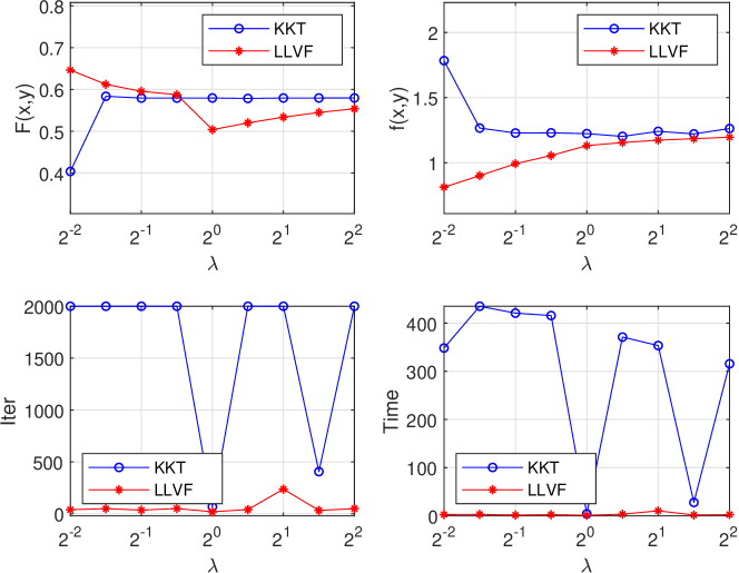
Figure 4. Performance of SNKKT and SNVF on solving the quadratic BOC program.

Finally, in order to estimate the local behaviour of SNKKT and SNVF on our test examples, we report on the experimental order of convergence (EOC) defined by

$$\mbox{EOC}:=\max\left\{\frac{\log\|\Phi^{\lambda}(\zeta^{K-1})\|}{\log\|\Phi^{\lambda}(\zeta^{K-2})\|},\,\frac{\log\|\Phi^{\lambda}(\zeta^{K})\|}{\log\|\Phi^{\lambda}(\zeta^{K-1})\|}\right\}.$$

As shown in Figure 3, when $\lambda=2^{-1}$, for examples, SNKKT (resp. SNVF) solves 27 (resp. 14) problems with $\mbox{EOC}<1.1$, 8 (resp. 9) problems with $1\leq\mbox{EOC}<1.5$ and 89 (resp. 101) examples with $\mbox{EOC}\geq 1.5$. Generally speaking, SNVF outperforms SNKKT because it solves more examples with $\mbox{EOC}\geq 1.5$ and fewer examples with $\mbox{EOC}<1.1$.

5.4. Comparison of SNKKT and SNVF on solving a quadratic BOC program

Note that the examples in the BOLIB library are of a small scale, with dimensions satisfying $\max\{n,m,p,q\}\leq 20$. Therefore, to see the performance of SNKKT and SNVF on solving problems with lager scale, we take advantage of a discretized bilevel optimal control (BOC) program from [26]. This is a quadratic program and its dimensions $\{n,m,p,q\}$ can to be altered. The model is described by

$$\begin{array}[]{rll}F(x,y)&:=&\frac{1}{2}[(y^{1};0)-c]^{\top}D[(y^{1};0)-c]-d^{\top}x,\\ G(x,y)&:=&\left(-x_{1}+x_{2}-1;-x\right),\\ f(x,y)&:=&\frac{1}{2}(Cy^{1}-Px)^{\top}U(Cy^{1}-Px)+\frac{\sigma}{2}(y^{2}-Qx)^{\top}V(y^{2}-Qx),\\ g(x,y)&:=&\left(y^{2}-u;-y^{2}+l;Ay;-Ay\right),\end{array}$$

where $x\in\mathbb{R}^{2}$, $y=(y^{1};y^{2})$ with $y^{i}\in\mathbb{R}^{m_{i}}$, $D\in\mathbb{R}^{m_{1}\times m_{1}}$, $d\in\mathbb{R}^{n}$, $c\in\mathbb{R}^{m}$, $C\in\mathbb{R}^{s\times m_{1}}$, $P\in\mathbb{R}^{s\times n}$, $U\in\mathbb{R}^{s\times s}$, $Q\in\mathbb{R}^{m_{2}\times n}$, $V\in\mathbb{R}^{m_{2}\times m_{2}}$, $u\in\mathbb{R}^{m_{2}}$, $l\in\mathbb{R}^{m_{2}}$, $A\in\mathbb{R}^{t\times m}$ are given data. Here, $(a;b)=(a^{\top}\leavevmode\nobreak\ b^{\top})^{\top}.$ For simplicity, we fix the dimensions as $n=2,m=274,p=3,m_{1}=m_{2}=s=t=137$ and thus $q=548$.

	$\lambda$	$2^{-2}$	$2^{-1.5}$	$2^{-1}$	$2^{-0.5}$	$2^{0}$	$2^{0.5}$	$2^{1}$	$2^{1.5}$	$2^{2}$
$F(x,y)$	SNKKT	0.40	0.58	0.58	0.58	0.58	0.58	0.58	0.58	0.58
	SNVF	0.65	0.61	0.60	0.59	0.50	0.52	0.53	0.54	0.55
$f(x,y)$	SNKKT	1.78	1.27	1.23	1.23	1.22	1.20	1.24	1.22	1.26
	SNVF	0.81	0.90	0.99	1.05	1.13	1.15	1.17	1.18	1.20
Iter	SNKKT	2000	2000	2000	2000	67	2000	2000	406	2000
	SNVF	39	49	35	50	19	40	237	32	49
Time	SNKKT	348.34	435.07	420.82	415.74	4.04	371.10	353.46	27.74	315.67
	SNVF	2.56	3.03	1.54	2.45	1.06	3.40	10.34	1.69	2.48
Time/Iter	SNKKT	0.17	0.22	0.21	0.21	0.06	0.19	0.18	0.07	0.16
	SNVF	0.07	0.06	0.04	0.05	0.06	0.08	0.04	0.05	0.05

Table 7. Performance of SNKKT and SNVF on solving the quadratic BOC program.

We now compare the performance of SNKKT and SNVF on solving a BOC program with larger size $n=2$, $m=274$, $p=3$, and $q=548$. The problem is quadratic, and thus there is no need to calculate the third derivatives of functions in lower level problem. We tested different values of $\lambda$ on solving this problem and observed that larger values $\lambda$ (e.g., $\lambda>4$) led to a bad performance for both methods. Therefore, we used $\lambda\in\{2^{-2},\;2^{-1.5},\ldots,2^{1.5},2^{2}\}$. As depicted in Figure 4, it can be clearly seen that SNVF outperforms SNKKT in terms of the number of iterations and the computing time. Most importantly, from the subfigure Iter, among 9 choices of $\lambda$, SNKKT used 2000 iterations for 7 choices of $\lambda$, which means it did not get desired solutions before it stopped. Detailed results were listed in Table 7. It seems that the best optimal upper level and lower level objective function values are 0.5 and 1.13, respectively. The last two rows reported the time per each iteration, in which SNVF ran much faster than SNKKT for all $\lambda$.

6. Conclusions and future work

In this work, we have considered the most common single-level reformulations of the bilevel optimization problem; i.e., problems (KKTR) and (LLVFR). After a detailed theoretical analysis and comparison of the two problems, in terms of (1) the requirements for problems to $\mathcal{C}^{1}$ or Lipschitz continuous and equivalent to the original problem (P), (2) the necessary optimality conditions and qualification conditions necessary to derive them, (3) frameworks for semismooth Newton-type method and convergence, and (4) numerical efficiency. It has resulted from the theoretical framework that non of the reformulations can be said to be superior to the other, although the KKT reformulation provides some higher level of flexibility and tractability that it borrows from the well-established field of MPCCs. However, from the numerical perspective, the LLVF reformulation appears to be superior to the KKT reformulation based the experiments conducted in this paper. Our assessment is that this may be largely due to the fact the size of the equation solved for the KKT reformulation is larger by $q\times q$ ($q$ number of lower-level constraints) and the fact that this reformulation is very sensitive to lower-level convexity and regularity condition as shown in [7] (see Subsection 2.1), while the LLVF reformulation is completely equivalent (i.e., globally and locally) to problem (P). Moreover, due to the presence of the gradient of lower-level Lagrangian function in the KKT reformulation, the evaluation of 3rd order derivatives of functions involved in the lower-level problem is required in the methods considered in this paper. The latter issue does not appear to have played a big influence in the test set used in this paper, but will be potentially be very detrimental to bilevel programs of lager sizes, especially when 3rd order derivatives of lower-level functions are nonzero. In order to check whether the observations made on the numerical performance of the methods studied in this paper for (KKTR) and (LLVFR) are valid in general, in a future work, we will be studying and comparing the theoretical performance bounds of the semismooth Newton-type method for both problems in a general setting.

References

- [1] J.F. Bard. Some properties of the bilevel programming problem, Journal of Optimization Theory and Applications 68(2):371–378, 1991.
- [2] J.F. Bard. Practical bilevel optimization: algorithms and applications, Kluwer Academic Publishers, 1998.
- [3] J.F. Bonnans and A. Shapiro. Perturbation analysis of optimization problems, Springer, 2000.
- [4] F.H. Clarke. Optimization and nonsmooth analysis, Wiley & Sons, 1983.
- [5] T. De Luca, F. Facchinei, and C. Kanzow. A semismooth equation approach to the solution of nonlinear complementarity problems, Mathematical Programming 75(3):407–439, 1996.
- [6] S. Dempe. Foundations of bilevel programming, Kluwer Academic Publishers, 2002.
- [7] S. Dempe and J. Dutta. Is bilevel programming a special case of mathematical programming with equilibrium constraints? Mathematical Programming 131 (1-2):37–48, 2012.
- [8] S. Dempe, J. Dutta, and B.S. Mordukhovich. New necessary optimality conditions in optimistic bilevel programming, Optimization 56(5-6):577–604, 2007.
- [9] S. Dempe and S. Franke. On the solution of convex bilevel optimization problems, Computational Optimization and Applications 63(3):685–703, 2016.
- [10] S. Dempe and S. Franke. Solution algorithm for an optimistic linear Stackelberg problem, Computers & Operations Research 41:277–281, 2014.
- [11] S. Dempe and S. Franke. Solution of bilevel optimization problems using the KKT approach, Optimization 68(8):1471–1489, 2019.
- [12] S. Dempe and A.B. Zemkoho. On the Karush-Kuhn-Tucker reformulation of the bilevel optimization problem, Nonlinear Analysis: Theory, Methods & Applications 75:1202–1218, 2012.
- [13] S. Dempe and A.B. Zemkoho. The generalized Mangasarian-Fromowitz constraint qualification and optimality conditions for bilevel programs, Journal of Optimization Theory and Applications 148:433–441, 2011.
- [14] A.V. Fiacco. Introduction to sensitivity and stability analysis in nonlinear programming, Academic press, 1983.
- [15] A. Fischer. A special Newton-type optimization method, Optimization 24(3-4):269–284, 1992.
- [16] A. Fischer, A.B. Zemkoho, and S.L. Zhou. Semismooth Newton-type method for bilevel optimization: Global convergence and extensive numerical experiments, arXiv:1912.07079, 2019.
- [17] A. Fischer, A.B. Zemkoho, and S.L. Zhou. Detailed numerical experiment for “Semismooth newton-type method for bilevel optimization: Global convergence and extensive numerical experiments”, Technical Report, School of Mathematics, University of Southampton, UK, 2019.
- [18] M.L. Flegel, C. Kanzow, and J.V. Outrata. Optimality conditions for disjunctive programs with application to mathematical programs with equilibrium constraints, Set-Valued Analysis 15(2):139-162, 2007.
- [19] A. Galántai. Properties and construction of NCP functions, Computational Optimization and Applications 52(3):805–824, 2012.
- [20] J. Gauvin and F. Dubeau. Differential properties of the marginal function in mathematical programming, Mathematical Programming Study 18:101–119, 1982.
- [21] R. Henrion and T. Surowiec. On calmness conditions in convex bilevel programming, Applicable Analysis 90(6):951-970.
- [22] H.T. Jongen, J.J. Rückmann, and O. Stein. Generalized semi-infinite optimization: a first order optimality condition and examples Mathematical Programming 83(1-3): 145–58, 1998.
- [23] L. Lampariello and S. Sagratella. A bridge between bilevel programs and Nash games, Journal of Optimization Theory and Applications 174(2):613-635, 2017.
- [24] L. Lampariello and S. Sagratella. Numerically tractable optimistic bilevel problems, Computational Optimization and Applications 76:277-303, 2020.
- [25] G.H. Lin, M. Xu, and J.J. Ye. On solving simple bilevel programs with a nonconvex lower level program, Mathematical Programming 144(1-2):277–305, 2014.
- [26] P. Mehlitz and G. Wachsmuth. Weak and strong stationarity in generalized bilevel programming and bilevel optimal control. Optimization 65:907–935, 2016.
- [27] P. Mehlitz, L.I. Minchenko, and A.B. Zemkoho. A note on partial calmness for bilevel optimization problems with linear structures at the lower level, arXiv:2003.06138, 2020.
- [28] P. Mehlitz and A.B. Zemkoho. Sufficient optimality conditions in bilevel programming, arXiv:1911.01647, 2019.
- [29] A.G. Mersha and S. Dempe. Feasible direction method for bilevel programming problem, Optimization 61(5):597-616, 2012.
- [30] R. Mifflin. Semismooth and semiconvex functions in constrained optimization, SIAM Journal on Control and Optimization 15(6):959–972, 1977.
- [31] B.S. Mordukhovich. Variational Analysis and Applications, Springer, 2018.
- [32] L. Qi. Convergence analysis of some algorithms for solving nonsmooth equations, Mathematics of Operations Research 18(1):227–244, 1993.
- [33] L. Qi and H. Jiang. Semismooth Karush-Kuhn-Tucker equations and convergence analysis of Newton and quasi-Newton methods for solving these equations, Mathematics of Operations Research 22(2):301–325, 1997.
- [34] L. Qi and D. Sun. A survey of some nonsmooth equations and smoothing Newton methods, in Progress in Optimization, pp. 121–146, Springer, 1999.
- [35] L. Qi and J. Sun. A nonsmooth version of Newton’s method, Mathematical Programming 58:353–367, 1993.
- [36] R.T. Rockafellar. Convex analysis, Princeton University Press, 1970.
- [37] R.T. Rockafellar and R.J.B. Wets. Variational analysis, Springer, 2009.
- [38] K.H. Sahin and A.R. Ciric. A dual temperature simulated annealing approach for solving bilevel programming problems, Computers and Chemical Engineering 23(1):11–25, 1998.
- [39] M. Xu and J.J. Ye. A smoothing augmented Lagrangian method for solving simple bilevel programs, Computational Optimization and Applications 59(1-2):353–377, 2014.
- [40] M. Xu, J.J. Ye, and L. Zhang. Smoothing SQP methods for solving degenerate nonsmooth constrained optimization problems with applications to bilevel programs, SIAM Journal on Optimization 25(3):1388–1410, 2015.
- [41] J.Y. Ye. Necessary and sufficient optimality conditions for mathematical programs with equilibrium constraints, Journal of Mathematical Analysis and Applications 307(1):350–369, 2005.
- [42] J.J. Ye and D. Zhu. New necessary optimality conditions for bilevel programs by combining the MPEC and value function approaches, SIAM Journal on Optimization 20(4):1885–1905, 2010.
- [43] J.J. Ye and D.L. Zhu. Optimality conditions for bilevel programming problems, Optimization 33:9–27, 1995 (with Erratum in Optimization 39:361–366, 1997).
- [44] J.J. Ye, D.L. Zhu, and Q.J. Zhu. Exact penalization and necessary optimality conditions for generalized bilevel programming problems, SIAM Journal on Optimization 7(2):481–507, 1997.
- [45] A.B. Zemkoho. Bilevel programming: reformulations, regularity, and stationarity, PhD thesis, Technical University Bergakademie Freiberg, Germany, 2012.
- [46] S.L. Zhou, A.B. Zemkoho, and A. Tin, BOLIB: Bilevel Optimization LIBrary of Test Problems, in S. Dempe and A.B. Zemkoho (eds). Bilevel optimization: advances and next challenges, Springer, 2020.