Spin-mediated Mott excitons

Abstract

Motivated by recent experiments on Mott insulators, in both iridates and ultracold atoms, we theoretically study the effects of magnetic order on the Mott-Hubbard excitons. In particular, we focus on spin-mediated doublon-holon pairing in Hubbard materials. We use several complementary theoretical techniques: mean-field theory to describe the spin degrees of freedom, the self-consistent Born approximation to characterize individual charge excitations across the Hubbard gap, and the Bethe-Salpeter equation to identify bound states of doublons and holons. The binding energy of the Mott exciton is found to increase with increasing the Néel order parameter, while the exciton mass decreases. We observe that these trends rely significantly on the retardation of the effective interaction, and require consideration of multiple effects from changing the magnetic order. Our results are consistent with the key qualitative trends observed in recent experiments on iridates. Moreover, the findings could have direct implications on ultracold atom Mott insulators, where the Hubbard model is the exact description of the system and the microscopic degrees of freedom can be directly accessed.

I Introduction

The physics of excitons in semiconductors, i.e., bound states of electrons and holes, is by now well-established Haug and Schmitt-Rink (1984); Haug and Koch (2004). Excitons play an essential role in technologies such as light-emitting diodes Burroughes et al. (1990), organic solar cells Gregg (2003), and photodetectors Itkis et al. (2006), among others. Furthermore, there has recently been tremendous interest in hybridizing exciton states with photon modes in optical cavities Carusotto and Ciuti (2013). Such exciton polaritons can form (non-equilibrium) Bose-Einstein condensates at remarkably high temperatures, even room temperature Kasprzak et al. (2006); Keeling et al. (2007); Deng et al. (2010); Byrnes et al. (2014); Plumhof et al. (2014).

Given these applications, it is important to study the properties of excitons in systems other than conventional semiconductors. It has been convincingly established that excitonic states do exist in strongly correlated materials such as Mott insulators Gallagher and Mazumdar (1997); Essler et al. (2001); Wróbel and Eder (2002); Matsueda et al. (2005); Ono et al. (2005); Gössling et al. (2008); Al-Hassanieh et al. (2008); Novelli et al. (2012); Gretarsson et al. (2013); Kim et al. (2014), yet essential aspects of Mott excitons remain poorly understood.

For example, it is known that Mott insulators are often antiferromagnetic at low temperature, but very little work has been done to understand how and to what extent the presence of such order affects exciton properties. The qualitative role of magnetization is sketched in Fig. 1 – charges remain bound so as to minimize the number of spins disrupted by their motion – but a quantitative description has been lacking.

Recent experiments have begun to investigate this question. In Refs. Alpichshev et al. (2015, 2017), pump-probe experiments were performed on the Mott insulator Na₂IrO₃ both with and without magnetic order (controlled by varying temperature or applying an intermediate pulse). The authors concluded that the binding energy and exciton mass are both enhanced by the presence of magnetization. Ref. Terashige et al. (2019) similarly observed that the binding energy increases with the spin-spin interaction strength in cuprates. See also Ref. Eckstein and Werner (2016), which found that the relaxation time in Mott insulators decreases with increasing spin correlations.

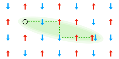
Figure 1: Sketch of the physics underlying spin-mediated exciton formation in a Mott insulator. A string of flipped spins (green line) connects the hole and double-occupancy. The energy cost associated to the string binds them together.

The same question can apply to Mott insulators in synthetic quantum systems, such as ultracold gases. By loading fermionic atoms into an optical lattice and tuning their interactions, the Fermi-Hubbard model can be synthesized experimentally Schneider et al. (2008); Bloch et al. (2008); Esslinger (2010); Bloch et al. (2012); Gross and Bloch (2017). Unlike condensed matter systems, such as the iridates, neutral fermionic atoms in an optical lattice are genuinely described by the Hubbard Hamiltonian, without any additional effects arising from longer-range Coulomb interactions, phonons, etc. Researchers have quite recently begun investigating the interplay of spin and charge degrees of freedom in this setting Parsons et al. (2016); Boll et al. (2016); Cheuk et al. (2016); Hilker et al. (2017); Salomon et al. (2019); Koepsell et al. (2019); Vijayan et al. (2020) (note that here the “charge” excitations are not actually charged).

In this paper, we perform a theoretical study of the role of magnetic order in Mott excitons, the first such to our knowledge. As depicted in Fig. 1, in an anti-ferromagnetic background, a hole and doubly occupied site can bind through a string of flipped spins. Such Mott excitons differ from conventional excitons formed by Coulomb interaction in two aspects. First, the spin-mediated interaction is far from instantaneous, and second, the individual charges are themselves renormalized by spin fluctuations. We shall demonstrate that both effects are necessary ingredients in the trends reported here.

Given the complexity of the problem, our analysis requires multiple stages. We first use slave particles to isolate spin and charge degrees of freedom, then describe the spin dynamics by mean-field theory, calculate the dispersion of charges self-consistently, and finally characterize excitonic states via the Bethe-Salpeter equation. Many of the steps in this program are analogous to those in Ref. Han et al. (2016), which studied charge dynamics in the Hubbard model. The good agreement between the results of Ref. Han et al. (2016) and alternate numerical methods lends support to the present approach.

Our key finding is that larger magnetization leads to an increased binding energy of the Hubbard exciton but a decreased mass. This observation is in some tension with interpretations of recent experiments Alpichshev et al. (2017). It also stands in contrast to conventional Coulomb-mediated excitons, where the binding energy and mass are proportional to each other.

Note that the formation of Mott excitons is closely related to the Cooper pairing of holes in high-$T_{c}$ superconductors. Similar treatments of hole-hole binding can be found in the corresponding literature Shraiman and Siggia (1989); Kuchiev and Sushkov (1993); Belinicher et al. (1995, 1997); Brügger et al. (2006). Nonetheless, there are differences between the two problems, as we discuss below. Moreover, to the best of our knowledge, a study of how the bound state properties change as a function of magnetization has not yet been carried out.

In the following Sec. II, we describe the steps of our analysis in detail. Results are presented in Sec. III, and Sec. IV concludes.

II Formalism & methods

Our starting point is the 2D Fermi-Hubbard model, which by now needs no introduction:

$$H_{\textrm{Hub}}=-t\sum_{\langle ij\rangle,\sigma}c_{i\sigma}^{{\dagger}}c_{j\sigma}+U\sum_{i}n_{i\uparrow}n_{i\downarrow},$$ (1)

where $\sigma\in\{\uparrow,\downarrow\}$ and $\langle ij\rangle$ denotes nearest-neighbor sites on a square lattice. $c_{i\sigma}$ is the usual electron annihilation operator and $n_{i\sigma}\equiv c_{i\sigma}^{{\dagger}}c_{i\sigma}$. We shall consider the system at half filling in the $U\gg t$ limit.

It is well-known that in this limit, the Hubbard model features two types of excitations, associated with the transport of charge and spin respectively Hirsch (1985); Kotliar and Ruckenstein (1986); White et al. (1989); Lee (1989). Furthermore, the charge excitations can be either positive or negative, corresponding to sites with zero or two electrons, and their creation comes with a large energy cost of order $U$. By analogy with conventional semiconductors, we thus expect this system to support well-defined excitons in the dilute-charge limit. However, long-wavelength spin excitations do not come with an energy cost, and their presence plays a significant role in determining the exciton properties.

There are many formalisms with which to study the Hubbard model Ogawa et al. (1975); MacDonald et al. (1988); Li et al. (1989); Lee et al. (2006). Since our focus is on the motion of only a few charges within a background of spin excitations, the slave-particle formalism is particularly well-suited Schmitt-Rink et al. (1988); Kane et al. (1989); Han et al. (2016). The steps of our calculation are as follows:

1. Express the Hamiltonian in terms of slave particles – doublons, holons, & spinons – and reduce to the t-J model following the standard procedure Auerbach (1994).

2. Treat the Heisenberg interaction within semiclassical and mean-field approximations, while neglecting the back action of doublons and holons on the magnetic order.

3. Calculate the dispersion of individual doublons and holons in the magnetic background via the self-consistent Born approximation.

4. Calculate exciton properties using the Bethe-Salpeter equation.

The major limitation of this program is our approximate description of the magnetic order. Thus we do not claim to have quantitatively accurate results, especially at small magnetization. That said, we do expect that the qualitative trends seen here are accurate, including near the equilibrium value of magnetization, for which mean field theory is known to work reasonably well (see Ref. Han et al. (2016) and references therein).

II.1 Slave particles

In the slave-particle formalism, we express the electron operator as (with $\sigma=\pm 1$)

$$c_{i\sigma}=s_{i,-\sigma}^{{\dagger}}d_{i}+\sigma e_{i}^{{\dagger}}s_{i\sigma},$$ (2)

where $d_{i}$ and $e_{i}$ are fermionic operators and $s_{i\sigma}$ is bosonic. One can confirm that Eq. (2) is consistent with the commutation relations. A site with a $d$ particle is to be interpreted as a site with two electrons (a “doublon”), a site with an $e$ particle is to be interpreted as an empty site (a “holon”), and a site with an $s_{\sigma}$ particle is one with a single electron having spin $\sigma$ (a “spinon”). See Fig. 2. The physical content of Eq. (2) is then clear: removing an electron of given spin is equivalent to replacing the doublon with the opposite spinon if the site is doubly-occupied and replacing the spinon with a holon if the site is singly-occupied (otherwise the state is annihilated). Note that since every site is in one of the four states – empty, spin-up, spin-down, doubly-occupied – there must be exactly one of the fictitious particles on each site:

$$d_{i}^{{\dagger}}d_{i}+e_{i}^{{\dagger}}e_{i}+s_{i\uparrow}^{{\dagger}}s_{i\uparrow}+s_{i\downarrow}^{{\dagger}}s_{i\downarrow}=1,\;\forall i.$$ (3)

The original Hamiltonian clearly preserves this relationship.

Substituting Eq. (2) into Eq. (1), we have that

$$H_{\textrm{Hub}}= -t\sum_{\langle ij\rangle,\sigma}\big{(}d_{i}^{{\dagger}}d_{j}-e_{i}^{{\dagger}}e_{j}\big{)}s_{j\sigma}^{{\dagger}}s_{i\sigma}+U\sum_{i}d_{i}^{{\dagger}}d_{i}$$ (4)

$$-t\sum_{\langle ij\rangle,\sigma}\sigma\big{(}d_{i}^{{\dagger}}e_{j}^{{\dagger}}s_{i,-\sigma}s_{j\sigma}+e_{i}d_{j}s_{i\sigma}^{{\dagger}}s_{j,-\sigma}^{{\dagger}}\big{)}.$$

Note that the first line preserves the number of doublons and holons, whereas the second line does not.

At large $U$, the second line of Eq. (4) can be treated by perturbation theory in $t/U$. The method as applied here is standard, and can be found in, e.g., Ref. Auerbach (1994). We obtain the t-J model:

$$H_{\textrm{tJ}}= -t\sum_{\langle ij\rangle,\sigma}\big{(}d_{i}^{{\dagger}}d_{j}-e_{i}^{{\dagger}}e_{j}\big{)}s_{j\sigma}^{{\dagger}}s_{i\sigma}+U\sum_{i}d_{i}^{{\dagger}}d_{i}$$ (5)

$$-J\sum_{\langle ij\rangle}\big{(}s_{i\uparrow}^{{\dagger}}s_{j\downarrow}^{{\dagger}}-s_{i\downarrow}^{{\dagger}}s_{j\uparrow}^{{\dagger}}\big{)}\big{(}s_{j\downarrow}s_{i\uparrow}-s_{j\uparrow}s_{i\downarrow}\big{)},$$

where $J\equiv 4t^{2}/U$. Strictly speaking, Eq. (5) should include additional next-nearest-neighbor terms, as well as a direct interaction between nearest-neighbor doublons and holons, but these are commonly neglected.

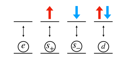
Figure 2: Sketch of the slave-particle formalism. Each of the four possible occupancies on a site corresponds to a different type of fictitious particle.

II.2 Magnetic ordering

The second line of Eq. (5) is precisely the antiferromagnetic Heisenberg Hamiltonian, expressed in terms of Schwinger bosons (here the spinons $s_{i\sigma}$) Auerbach (1994). We are specifically considering Néel-ordered ground states, with positive magnetization on the $A$ sublattice and negative on $B$. It is thus convenient to express $s_{i\uparrow}$ ($s_{i\downarrow}$) in terms of $s_{i\downarrow}$ ($s_{i\uparrow}$) for $i\in A$ ($B$), using Eq. (3) — this is equivalent to using Holstein-Primakoff rather than Schwinger bosons Auerbach (1994):

$$s_{i\uparrow} =\left[1-s_{i\downarrow}^{{\dagger}}s_{i\downarrow}\right]^{1/2},\quad i\in A,$$ (6)

$$s_{i\downarrow} =\left[1-s_{i\uparrow}^{{\dagger}}s_{i\uparrow}\right]^{1/2},\quad i\in B.$$

We neglect $d_{i}^{{\dagger}}d_{i}$ and $e_{i}^{{\dagger}}e_{i}$ in using Eq. (3) because we are interested in the dilute-charge limit. From here on, we shall simply write $s_{i}$ in place of $s_{i\downarrow}$ ($s_{i\uparrow}$) for $i\in A$ ($B$). On both sublattices, the $s_{i}$ boson represents a fluctuation relative to perfect Néel order.

Note that Eq. (6) cannot be an exact equality because it does not respect the fact that $[s_{i\sigma},s_{i\sigma}^{{\dagger}}]=1$. It is more of a semiclassical approximation, valid in the limit of large spin $S$. Of course, the case $S=1/2$ under consideration here is far from large, but all other analytical techniques of which we are aware for treating long-range order via slave particles (such as Bose-Einstein condensation of the Schwinger bosons Sarker et al. (1989, 1990)) have the same regime of validity. We refer for Ref. Auerbach (1994) for more details.

Inserting Eq. (6) into $H_{\textrm{tJ}}$ does not yield a solvable Hamiltonian on its own. Thus to progress further, we make a mean-field approximation by expanding $H_{\textrm{tJ}}$ to first order in $s_{i}^{{\dagger}}s_{i}-\langle s_{i}^{{\dagger}}s_{i}\rangle$ (this is also reasonable in the semiclassical limit). With $\langle s_{i}^{{\dagger}}s_{i}\rangle=1/2-m$, where $m$ is the Néel magnetization, we find that

$$H_{\textrm{tJ}}\approx -\sqrt{\frac{1+2m}{2}}t\sum_{\langle ij\rangle}\big{(}d_{i}^{{\dagger}}d_{j}-e_{i}^{{\dagger}}e_{j}\big{)}\big{(}s_{i}+s_{j}^{{\dagger}}\big{)}$$ (7)

$$+4(1+2m)J\sum_{i}s_{i}^{{\dagger}}s_{i}+\frac{1+2m}{2}J\sum_{\langle ij\rangle}\big{(}s_{i}^{{\dagger}}s_{j}^{{\dagger}}+s_{i}s_{j}\big{)}$$

$$+U\sum_{i}d_{i}^{{\dagger}}d_{i}-NJ(1+2m)^{2}.$$

The second line is diagonalized by passing to momentum space and performing a Bogoliubov transformation, leading to the final Hamiltonian (neglecting constant terms)

$$H_{\textrm{tJ}}\approx -\sqrt{\frac{1+2m}{2N}}t\sum_{kq}d_{k+q}^{{\dagger}}d_{k}\big{(}M_{kq}\beta_{q}+M_{k+q,-q}\beta_{-q}^{{\dagger}}\big{)}$$ (8)

$$+\sqrt{\frac{1+2m}{2N}}t\sum_{kq}e_{k+q}^{{\dagger}}e_{k}\big{(}M_{kq}\beta_{q}+M_{k+q,-q}\beta_{-q}^{{\dagger}}\big{)}$$

$$+U\sum_{q}d_{q}^{{\dagger}}d_{q}+\sum_{q}\omega_{q}\beta_{q}^{{\dagger}}\beta_{q},$$

where the sum is over the 2D Brillouin zone ($N$ is the number of lattice sites) and $\beta_{q}\equiv u_{q}s_{q}+v_{q}s_{-q}^{{\dagger}}$ is the transformed spinon operator. With

$$u_{q}\equiv\sqrt{\frac{1}{2}\left(1+\frac{1}{\sqrt{1-\gamma_{q}^{2}}}\right)},$$ (9)

$$v_{q}\equiv\textrm{sgn}[\gamma_{q}]\sqrt{\frac{1}{2}\left(\frac{1}{\sqrt{1-\gamma_{q}^{2}}}-1\right)},$$ (10)

where

$$\gamma_{q}\equiv\frac{1}{2}\big{(}\cos{q_{x}}+\cos{q_{y}}\big{)},$$ (11)

the frequencies $\omega_{q}$ and vertices $M_{kq}$ entering into Eq. (8) are given by

$$\omega_{q}=4(1+2m)J\sqrt{1-\gamma_{q}^{2}},$$ (12)

$$M_{kq}=4\gamma_{k}u_{q}-4\gamma_{k+q}v_{q}.$$ (13)

Normally one would determine $m$ self-consistently from the ground state spinon occupation: $1/2-m=N^{-1}\sum_{q}\langle s_{q}^{{\dagger}}s_{q}\rangle=N^{-1}\sum_{q}v_{q}^{2}$. This is known to give $m\approx 0.3$ for a 2D square lattice Han et al. (2016). We shall instead treat $m$ as an independent parameter — this is an approximate (albeit crude) means of estimating exciton properties as a function of magnetization.

II.3 Self-consistent Born approximation

The self-consistent Born approximation (SCBA) gives the doublon-doublon and holon-holon propagators by the integral equation in Fig. 3. The same equation holds for each propagator separately. This approximation is expected to be accurate in the dilute-charge limit, where the charge dynamics is strongly affected by spinons but not vice-versa.

In terms of the doublon/holon self-energy $\Sigma_{k}(\epsilon)$, Fig. 3 translates to (after a frequency integration)

$$\Sigma_{k}(\epsilon)=\frac{(1+2m)t^{2}}{2N}\sum_{q}\frac{M_{kq}^{2}}{\epsilon-\omega_{q}-\Sigma_{k-q}(\epsilon-\omega_{q})}.$$ (14)

The quasiparticle spectrum $\epsilon_{k}$ is given by the solution to $\Sigma_{k}(\epsilon_{k})=\epsilon_{k}$.

Eq. (14) can be solved quite efficiently. Note that all $\omega_{q}$ are positive , thus Eq. (14) in fact expresses $\Sigma_{k}(\epsilon)$ in terms of the self-energy at lower frequencies. We start at sufficiently negative $\epsilon$, below which we approximate $\Sigma_{k}(\epsilon)\approx(1+2m)t^{2}/2N\sum_{q}M_{kq}^{2}/(\epsilon-\omega_{q})$, and then compute the self-energy at incrementally higher frequencies in terms of the previous values. To help avoid numerical errors, we add a small imaginary part (namely $0.1i(1+2m)J$) to $\epsilon$.

While one could proceed using the full $\Sigma_{k}(\epsilon)$, it has been found that the quasiparticle dispersion can be well-approximated by the form Martinez and Horsch (1991)

$$\epsilon_{k}= \,-2t_{1}\big{(}\cos{(k_{x}+k_{y})}+\cos{(k_{x}-k_{y})}\big{)}$$ (15)

$$\quad-2t_{2}\big{(}\cos{(2k_{x})}+\cos{(2k_{y})}+2\big{)}.$$

This expression has a clear physical interpretation: $t_{1}$ is the amplitude for performing a two-step hop along the diagonals of the lattice, and $t_{2}$ is the amplitude for a two-step hop along the principal axes (see Fig. 4). Thus in what follows, we shall use for the single-particle propagators the simpler expression

$$G_{k}(\epsilon)=\frac{1}{\epsilon-(1-i0)\epsilon_{k}},$$ (16)

with $\epsilon_{k}$ given by Eq. (15).

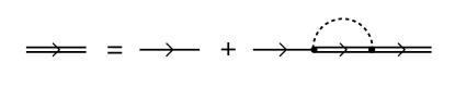
Figure 3: The self-consistent Born approximation (SCBA) for the single-particle propagator (either doublon-doublon or holon-holon). The solid single line is the free propagator, in this case simply $G_{k}^{0}(\epsilon)=1/\epsilon$, and the solid double line is the full propagator. The dashed line is the spinon propagator and the black dot is the vertex, corresponding to the Hamiltonian in Eq. (8).

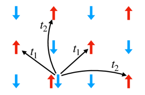
Figure 4: Illustration of hopping parameters $t_{1}$ and $t_{2}$ for the approximation to the quasiparticle dispersion in Eq. (15). Singly-occupied sites show the background magnetic order in which the double occupancy hops.

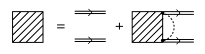
Figure 5: The integral equation which determines the two-particle Green’s function, within the ladder approximation. The hatched square is the Green’s function, and all other symbols are as in Fig. 3.

II.4 Bethe-Salpeter equation

We next consider the two-particle Green’s function ($T$ denotes time ordering)

$$\mathcal{G}_{j_{d}j_{e};j_{d}^{\prime}j_{e}^{\prime}}(t_{d},t_{e};t_{d}^{\prime},t_{e}^{\prime})$$ (17)

$$\qquad\quad\equiv-\big{<}Td_{j_{d}}(t_{d})e_{j_{e}}(t_{e})e_{j_{e}^{\prime}}(t_{e}^{\prime})^{{\dagger}}d_{j_{d}^{\prime}}(t_{d}^{\prime})^{{\dagger}}\big{>},$$

and its Fourier transform $\mathcal{G}_{k_{d}k_{e};k_{d}^{\prime}k_{e}^{\prime}}(\epsilon_{d},\epsilon_{e};\epsilon_{d}^{\prime},\epsilon_{e}^{\prime})$. Due to translational invariance, $\mathcal{G}$ depends only on differences in position and time, which we choose to parametrize by the relative coordinates

$$j\equiv \;j_{d}-j_{e},$$ (18)

$$j^{\prime}\equiv \;j_{d}^{\prime}-j_{e}^{\prime},$$

$$r\equiv \;\frac{j_{d}+j_{e}}{2}-\frac{j_{d}^{\prime}+j_{e}^{\prime}}{2},$$

with relative times defined analogously. The corresponding momenta are

$$k= \;\frac{k_{d}-k_{e}}{2},$$ (19)

$$k^{\prime}= \;\frac{k_{d}^{\prime}-k_{e}^{\prime}}{2},$$

$$K= \;k_{d}+k_{e}=k_{d}^{\prime}+k_{e}^{\prime}.$$

We will use absolute and relative momenta interchangeably, depending on notational convenience, with Eq. (19) always giving the relationship between the two. $\mathcal{G}_{k_{d}k_{e};k_{d}^{\prime}k_{e}^{\prime}}(\epsilon_{d},\epsilon_{e};\epsilon_{d}^{\prime},\epsilon_{e}^{\prime})$ will often be written as $\mathcal{G}_{kk^{\prime};K}(\epsilon,\epsilon^{\prime};E)$.

Within the ladder approximation, $\mathcal{G}$ is determined by the integral equation of Fig. 5. Written out,

$$\mathcal{G}_{kk^{\prime};K}(\epsilon,\epsilon^{\prime};E)=G_{k_{d}}(\epsilon_{d})G_{k_{e}}(\epsilon_{e})\Bigg{[}\delta_{kk^{\prime}}\,+\,\frac{(1+2m)t^{2}}{2N}\sum_{q}\int\frac{\textrm{d}\omega}{2\pi i}\left(\frac{M_{k_{d}-q,q}M_{k_{e},q}}{\omega-(1-i0)\omega_{q}}-\frac{M_{k_{d},-q}M_{k_{e}+q,-q}}{\omega+(1-i0)\omega_{q}}\right)\mathcal{G}_{k-q,k^{\prime};K}(\epsilon-\omega,\epsilon^{\prime};E)\Bigg{]},$$ (20)

where $G_{k}(\epsilon)$ is given by Eq. (16) and the vertices $M_{kq}$ are as in Eq. (8).

Since our goal is to identify bound states, we reduce Eq. (20) to the Bethe-Salpeter equation. The details of this approach can be found in Ref. Nakanishi (1969). We assume that $\mathcal{G}$ has an isolated pole in the total energy $E$, near which it has the form

$$\mathcal{G}_{kk^{\prime};K}(\epsilon,\epsilon^{\prime};E)\sim-i\frac{\psi_{k}(\epsilon)\overline{\psi}_{k^{\prime}}(\epsilon^{\prime})}{E-(1-i0)E_{b}},$$ (21)

where the “wavefunction” $\psi_{k}(\epsilon)$, its time-reversed partner $\overline{\psi}_{k}(\epsilon)$, and the bound state energy $E_{b}$ remain to be determined. Inserting this ansatz into both sides of Eq. (20) and equating the residues at $E_{b}$ on each side, we obtain a non-linear eigenvalue problem (the Bethe-Salpeter equation):

$$\psi_{k}(\epsilon)=G_{k_{d}}\left(\frac{E_{b}}{2}+\epsilon\right)G_{k_{e}}\left(\frac{E_{b}}{2}-\epsilon\right)\frac{(1+2m)t^{2}}{2N}\sum_{q}\int\frac{\textrm{d}\omega}{2\pi i}\left(\frac{M_{k_{d}-q,q}M_{k_{e},q}}{\omega-(1-i0)\omega_{q}}-\frac{M_{k_{d},-q}M_{k_{e}+q,-q}}{\omega+(1-i0)\omega_{q}}\right)\psi_{k-q}(\epsilon-\omega).$$ (22)

$E_{b}$ and $\psi_{k}(\epsilon)$ are given by the solution to Eq. (22). Note that they will depend on the center-of-mass momentum $K$.

$\psi_{k}(\epsilon)$ is the bound state wavefunction in a quite literal sense: it is the Fourier transform of

$$\psi_{j}(t)=\langle 0|Td_{j}(t)e_{0}(0)|b\rangle,$$ (23)

where $|b\rangle$ denotes the bound state and $|0\rangle$ denotes the ground state. Note that $t=0$ is of particular interest, since it gives the amplitude for simultaneously observing the holon at site 0 and the doublon at site $j$. Thus to simplify the problem, we integrate Eq. (22) over $\epsilon$, and furthermore, make the ansatz

$$\psi_{k}(\epsilon)=-G_{k_{d}}\left(\frac{E_{b}}{2}+\epsilon\right)G_{k_{e}}\left(\frac{E_{b}}{2}-\epsilon\right)\big{(}E_{b}-\epsilon_{k_{d}}-\epsilon_{k_{e}}\big{)}\Psi_{k},$$ (24)

with $\Psi_{k}$ independent of $\epsilon$. The explicit factor of $E_{b}-\epsilon_{k_{d}}-\epsilon_{k_{e}}$ is included so that $\Psi_{k}$ is the equal-time wavefunction, i.e., $\Psi_{k}=\psi_{k}(t=0)$. This ansatz allows us to perform the $\epsilon$ integral straightforwardly, giving a closed equation for $E_{b}$ and $\Psi_{k}$:

$$\big{(}E_{b}-\epsilon_{k_{d}}-\epsilon_{k_{e}}\big{)}\Psi_{k}=-\frac{(1+2m)t^{2}}{2N}\sum_{q}\left(\frac{M_{k_{d}-q,q}M_{k_{e},q}}{E_{b}-\epsilon_{k_{d}-q}-\omega_{q}-\epsilon_{k_{e}}}+\frac{M_{k_{d},-q}M_{k_{e}+q,-q}}{E_{b}-\epsilon_{k_{d}}-\epsilon_{k_{e}+q}-\omega_{q}}\right)\Psi_{k-q}.$$ (25)

Eq. (25) is the two-particle Schrodinger equation albeit with an energy-dependent potential. We find the values of $E_{b}$ at which it has a non-zero solution, and record the corresponding eigenvector.

Strictly speaking, Eq. (24) is not a valid ansatz for $\psi_{k}(\epsilon)$, i.e., it does not solve the frequency-dependent Eq. (22). However, it has a clear physical interpretation. The Fourier transform $\psi_{k}(t)$ gives the wavefunction for inserting the doublon and holon separated by time $t$ (see Eq. (23)). The poles coming from the single-particle propagators in Eq. (24) correspond to the phase factor acquired by the remaining particle during that interval, and our ansatz amounts to neglecting any other time dependence. This approximation has been applied previously to study holon-holon binding Belinicher et al. (1997), and we expect it to be qualitatively accurate for our purposes.

Eq. (25) and those preceding it differ from the equations for holon-holon binding in two respects. First, the holon-holon equations must include exchange terms not found here. Second, due to the relative phase between the doublon-spinon and holon-spinon vertices, the effective potential in Eq. (25) would have the opposite sign for the holon-holon problem.

III Results

III.1 Single-particle properties

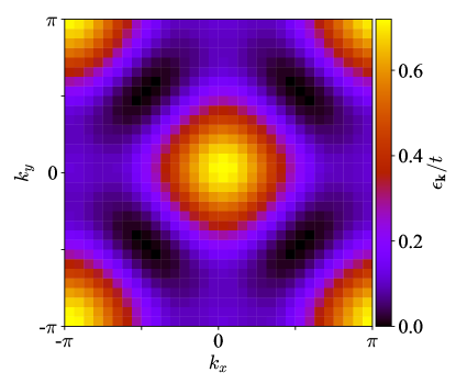
Figure 6: Dispersion of individual quasiparticles (both doublons and holons) within the SCBA, for a lattice of size $32\times 32$. Data shown is for $t/J=2$, $m=0.3$.

We first review the behavior of individual quasiparticles, determined within the SCBA as described above. Although these calculations have been reported previously, e.g., in Refs. Schmitt-Rink et al. (1988); Martinez and Horsch (1991), it will be useful to reproduce them here.

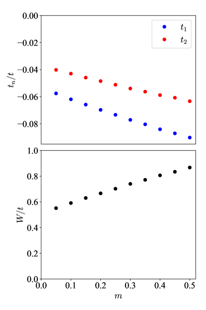
Figure 7: (Top) Fitted parameters of the quasiparticle dispersion (Eq. (15)) as a function of magnetization, for a lattice of size $32\times 32$ with $t/J=2$. (Bottom) Quasiparticle bandwidth versus magnetization for the same system.

Fig. 6 shows the quasiparticle dispersion throughout the Brillouin zone, with the magnetization set to the equilibrium value for concreteness. As noted above, it can be well-approximated by a next-nearest-neighbor hopping model with amplitude $t_{1}$ for moving along the diagonals of the lattice and amplitude $t_{2}$ for moving along the principal axes (see Fig. 4). The form of the dispersion is not sensitive to the value of magnetization. However, the effective hopping amplitudes, which we determine empirically by fitting the computed spectrum to Eq. (15), do depend on $m$ as shown in Fig. 7.

Some features of the dispersion can be explained by a simple Hartree-Fock approximation to the original Hamiltonian, in which the Hubbard interaction is replaced by $n_{i\uparrow}\langle n_{i\downarrow}\rangle+\langle n_{i\uparrow}\rangle n_{i\downarrow}$. Assuming Néel order for $\langle n_{i\sigma}\rangle$, the Hamiltonian becomes a tight-binding model on a bipartite lattice with dispersion

$$\epsilon_{k}^{\textrm{(HF)}}= \,\sqrt{U^{2}+4t^{2}\big{(}\cos{k_{x}}+\cos{k_{y}}\big{)}^{2}}$$ (26)

$$\sim \;U+\frac{2t^{2}}{U}\big{(}\cos{k_{x}}+\cos{k_{y}}\big{)}^{2},$$

using that $t\ll U$. Up to a constant shift, the second line is equivalent to Eq. (15) for the special case $t_{1}=2t_{2}$. Note in particular that $t_{1},t_{2}<0$. Thus Hartree-Fock correctly predicts that the band minimum is within the lines $k_{k}+k_{y}=\pm\pi$. It also correctly suggests that the bandwidth should be significantly reduced to $O(J)$ instead of $O(t)$. However, it incorrectly claims that the dispersion is degenerate along the entire magnetic Brillouin zone boundary. The more sophisticated SCBA resolves this degeneracy, identifying four minima at $(k_{x},k_{y})=(\pm\pi/2,\pm\pi/2)$.

Recent work on magnetic polarons in the t-J model Grusdt et al. (2019); Bohrdt et al. (2020) has made clear that this behavior can be understood by the charge excitations forming spinon-charge bound states (the “polarons”), held together by strings of displaced spins (much as we have sketched in Fig. 1 but with individual charges). The charges are forced to move on the timescale set by their slower spinon partners, namely $O(1/J)$, and are subject to the bipartite lattice felt by the spinons. The dispersion results shown above confirm this string picture quite nicely if one interprets them as being for the polaron as a whole. With that in mind, it is rather striking that these three approaches — SCBA, Hartree-Fock, and the string picture — all lead to consistent conclusions.

Returning to Fig. 7, we see that the bandwidth $W$ increases noticeably as the magnetization increases. Equivalently, the single-particle mass decreases. Within the framework of our calculation, the explanation is clear: a doublon/holon can move only if a spinon takes its place (see Eq. (5)), and since one spinon factor is always in the direction of the Néel magnetization, the doublon/holon hopping term is proportional to $\sqrt{(1+2m)/2}$.

III.2 Exciton properties

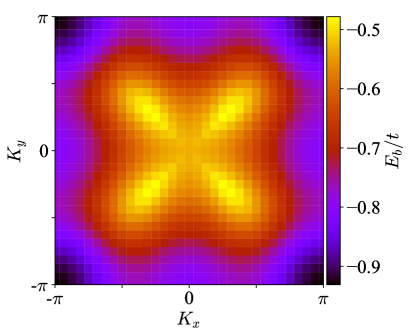
Figure 8: Dispersion of the exciton center-of-mass motion, for a lattice of size $32\times 32$. Data shown is for $t/J=2$, $m=0.3$.

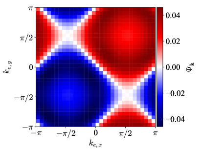
Figure 9: Exciton wavefunction in (relative) momentum space at total momentum $(K_{x},K_{y})=(\pi,\pi)$, for the same system as in Fig. 8.

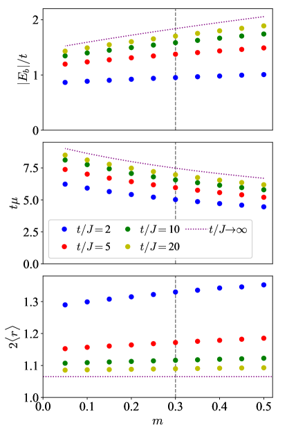
Figure 10: Exciton properties as functions of magnetization $m$, for various $t/J$ and a lattice of size $32\times 32$. The $t/J\rightarrow\infty$ curves are obtained from Eq. (27). Vertical dashed lines indicate the equilibrium value of $m$. (Top) Binding energy. (Center) Mass. (Bottom) Diameter.

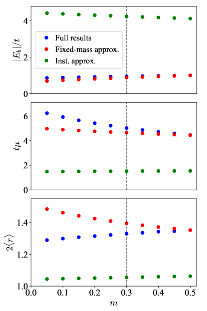
Figure 11: Comparison between the full results and the two approximations considered in the text. Data shown is for $t/J=2$ and a lattice of size $32\times 32$. Vertical dashed lines indicate the equilibrium value of $m$. For the fixed-mass points, the values of $t_{1}$ and $t_{2}$ are set to their values at $m=0.5$ (see Fig. 7).

We now turn to the exciton properties as functions of magnetization, using the Bethe-Salpeter equation. All of the quantities presented here are straightforward to compute from the energy $E_{b}$ and wavefunction $\psi_{k}$ given by Eq. (22).

Fig. 8 shows the energy of the lowest internal state as a function of the center-of-mass momentum $K$. As was the case for the single-particle dispersion, the shape of the exciton dispersion is not particularly sensitive to the magnetization. Note that the bottom of the band is not at the origin but rather at $(K_{x},K_{y})=(\pi,\pi)$. The wavefunction of the $(\pi,\pi)$ state is shown in Fig. 9. We see that it has $p$-wave symmetry, unlike what one would expect for a two-holon bound state.

The binding energy, mass, and radius of the exciton are plotted versus magnetization in Fig. 10. We see that as one increases the magnetization $m$, the mass decreases while the binding energy and size increase. It is interesting to compare these trends with what one would expect for a conventional exciton formed via Coulomb attraction. In that situation, a decrease in mass is associated with an increase in radius and a decrease in binding energy. Here, we find a similar relationship between radius and mass, but the binding energy instead scales inversely with mass.

Eq. (25) can be simplified further in the large-$t/J$ limit. We will see that $E_{b}$ scales as $t$, whereas $\epsilon_{k}$ and $\omega_{q}$ are asymptotically smaller Martinez and Horsch (1991). Thus we can neglect the single-particle and spinon dispersions, leaving the equation

$$E_{b}^{2}\Psi_{k}= -\frac{(1+2m)t^{2}}{2N}\sum_{q}\big{(}M_{k_{d}-q,q}M_{k_{e},q}$$ (27)

$$\qquad\qquad\qquad\qquad+M_{k_{d},-q}M_{k_{e}+q,-q}\big{)}\Psi_{k-q}.$$

Although still not of the Schrodinger form, Eq. (27) is much simpler to solve than Eq. (25): the kernel on the right-hand side no longer depends self-consistently on the energy (and as claimed, $E_{b}\sim t$). The results obtained from the large-$t/J$ equation are plotted alongside the others in Fig. 10.

As is clear from Eq. (25), the spinon-mediated interaction between charges is not instantaneous. To assess the importance of this retardation, we have compared the results in Fig. 10 to what would be obtained through the static approximation (setting $\omega=0$ in the kernel of Eq. (22)). The static approximation would predict significantly different results, as seen in Fig. 11: the binding energy would instead decrease slightly with magnetization and the mass would increase slightly. Thus the retardation of the effective interaction is an essential ingredient to the behavior seen here.

Similarly, one can ask whether the trends observed in Fig. 10 are due primarily to changes in the spinon behavior or rather due to the single-particle mass, which itself decreases with magnetization. We have repeated the above calculations under “fixed-mass” conditions, in which the single-particle parameters $t_{1}$ and $t_{2}$ are kept fixed (to their values at $m=0.5$) as we vary the magnetization. Fig. 11 shows that each of the three observables responds differently. The binding energy becomes more sensitive to magnetization, indicating that the quasiparticle and spinon properties play antagonistic roles. On the other hand, the exciton mass becomes less sensitive – the change to the effective interaction suppresses the mass by itself. Finally, the exciton radius shows the reverse behavior to before, instead decreasing with magnetization (although the size remains quite small in absolute terms).

The recent pump-probe experiments in Refs. Alpichshev et al. (2015, 2017) have investigated how excitons are influenced by magnetic order in the Mott insulator Na₂IrO₃. Our results support their interpretation in some aspects but not in others. In Ref. Alpichshev et al. (2015), the authors observe an increase in the fraction of bound excitations when below the Néel temperature, which they attribute to an increase in the exciton binding energy. Fig. 10 shows that magnetic order does indeed increase the binding energy. On the other hand, Ref. Alpichshev et al. (2017) demonstrates that the relaxational dynamics following a pump are slower in the presence of magnetic order. This is attributed to the mass increasing with magnetization, yet we have observed the opposite (consistent with past works calculating the dependence on $J/t$ Kane et al. (1989); von Szczepanski et al. (1990); Martinez and Horsch (1991)). Given the highly non-equilibrium nature of the experiments, as well as the approximations inherent in an analytical approach, further investigation is clearly needed.

Finally, let us compare the present calculation of doublon-holon binding to that of holon-holon binding, which is obviously of significant interest in its own right Lee et al. (2006); Plakida (2010). Clearly the two have much in common, yet there are two important differences. First, the integral equation which determines the two-particle Green’s function (Fig. 5) has an additional exchange term due to the indistinguishability of the holons. Second, even the direct term comes with an extra minus sign, i.e., the effective interaction is of opposite sign. The sign can be removed by redefining the hole operator on one sublattice, but the additional phase may modify further results depending on the application. It is important to keep these distinctions in mind when relating the present results to the high-$T_{c}$ literature.

IV Conclusion

We have studied the role that magnetic order plays in the formation of excitons within Mott insulators, using the Hubbard model as a concrete Hamiltonian. The binding energy increases in the presence of (antiferromagnetic) magnetization, whereas the exciton mass decreases. The size of the exciton increases slightly, yet the radius is never more than a lattice spacing. Using the standard classification, these are Frenkel excitons regardless of magnetic order.

In addition, we have established that the trends observed here require a detailed understanding of the many-body dynamics in these systems. Retardation effects in the effective spinon-mediated interaction are essential. Furthermore, the constituent charge and spin excitations are each affected separately by the background magnetic order, in ways cooperative for some exciton properties but antagonistic for others.

It must be noted that despite the complexity, there are significant limitations to our approach. In particular, we have made approximations in the spirit of linear spin-wave theory, which is only justified at large spin $S$ and full magnetization (neither of which we assume here). Thus we do not expect these results to be quantitatively accurate — we instead view this analysis as expressing our physical intuition regarding Mott excitons in the language of slave particles, from which we can make sharp predictions to be verified or falsified by more systematic investigations.

As an outlook, the predictions made here will be important when analyzing recent and future experiments on the optical properties of strongly correlated electronic materials. The existing experiments are quite complex, and require interpretations of their own. Our results agree with those interpretations in some respects but disagree in others. A complete understanding of the systems will require numerous approaches, both experimental and theoretical, including but not limited to the one described here.

Particularly promising are the recent experiments on fermionic atoms in optical lattices Hilker et al. (2017); Salomon et al. (2019); Vijayan et al. (2020). Since ultracold gases do not have many of the complicating features found in condensed matter systems, we expect that this will be a valuable direction to explore further. It is also likely that our conclusions, being based on the single-band nearest-neighbor Hubbard model, are more applicable to those systems than to materials such as the iridates. Importantly, current quantum gas microscopes allow one to directly create localized doublons and holons via optical tweezers, and reliably measure the spin correlation functions Koepsell et al. (2019). Such an unprecedented direct access to the system microscopics will provide a powerful way of investigating many-body excitons.

V Acknowledgements

We would like to thank Eugene Demler, Immanuel Bloch, Andrew Allocca, Zachary Raines, Yang-Zhi Chou, Fabian Grudst, and Annabelle Bohrdt for stimulating discussions and suggestions. This work was supported by the NSF Physics Frontier Center at the Joint Quantum Institute, the NSF DMR-1613029 and US-ARO contracts W911NF1310172 (T.-S.H), W911NF2010232, NRC Research Associateship award at the National Institute of Standards and Technology (CLB), AFOSR-MURI FA9550-16-1-0323 (M.H.), DOE-BES award DESC0001911 (V.G.) and the Simons Foundation. M.H. & V.G. acknowledge the hospitality of KITP-UCSB, which is supported in part by Grant No. NSF PHY-1748958.

References

- Haug and Schmitt-Rink (1984) H. Haug and S. Schmitt-Rink, “Electron theory of the optical properties of laser-excited semiconductors,” Progress in Quantum Electronics 9, 3 – 100 (1984).
- Haug and Koch (2004) H. Haug and S. W. Koch, Quantum Theory of the Optical and Electronic Properties of Semiconductors (World Scientific, 2004).
- Burroughes et al. (1990) J. H. Burroughes, D. D. C. Bradley, A. R. Brown, R. N. Marks, K. Mackay, R. H. Friend, P. L. Burns, and A. B. Holmes, “Light-emitting diodes based on conjugated polymers,” Nature 347, 539–541 (1990).
- Gregg (2003) Brian A. Gregg, “Excitonic solar cells,” The Journal of Physical Chemistry B 107, 4688–4698 (2003).
- Itkis et al. (2006) Mikhail E. Itkis, Ferenc Borondics, Aiping Yu, and Robert C. Haddon, “Bolometric infrared photoresponse of suspended single-walled carbon nanotube films,” Science 312, 413–416 (2006).
- Carusotto and Ciuti (2013) Iacopo Carusotto and Cristiano Ciuti, “Quantum fluids of light,” Rev. Mod. Phys. 85, 299–366 (2013).
- Kasprzak et al. (2006) J. Kasprzak, M. Richard, S. Kundermann, A. Baas, P. Jeambrun, J. M. J. Keeling, F. M. Marchetti, M. H. Szymańska, R. André, J. L. Staehli, V. Savona, P. B. Littlewood, B. Deveaud, and Le Si Dang, “Bose–einstein condensation of exciton polaritons,” Nature 443, 409–414 (2006).
- Keeling et al. (2007) J Keeling, F M Marchetti, M H Szymańska, and P B Littlewood, “Collective coherence in planar semiconductor microcavities,” Semiconductor Science and Technology 22, R1–R26 (2007).
- Deng et al. (2010) Hui Deng, Hartmut Haug, and Yoshihisa Yamamoto, “Exciton-polariton bose-einstein condensation,” Rev. Mod. Phys. 82, 1489–1537 (2010).
- Byrnes et al. (2014) Tim Byrnes, Na Young Kim, and Yoshihisa Yamamoto, “Exciton–polariton condensates,” Nature Physics 10, 803 EP – (2014).
- Plumhof et al. (2014) Johannes D. Plumhof, Thilo Stöferle, Lijian Mai, Ullrich Scherf, and Rainer F. Mahrt, “Room-temperature bose–einstein condensation of cavity exciton–polaritons in a polymer,” Nature Materials 13, 247–252 (2014).
- Gallagher and Mazumdar (1997) F. B. Gallagher and S. Mazumdar, “Excitons and optical absorption in one-dimensional extended hubbard models with short- and long-range interactions,” Phys. Rev. B 56, 15025–15039 (1997).
- Essler et al. (2001) F. H. L. Essler, F. Gebhard, and E. Jeckelmann, “Excitons in one-dimensional mott insulators,” Phys. Rev. B 64, 125119 (2001).
- Wróbel and Eder (2002) P. Wróbel and R. Eder, “Excitons in mott insulators,” Phys. Rev. B 66, 035111 (2002).
- Matsueda et al. (2005) H. Matsueda, T. Tohyama, and S. Maekawa, “Excitonic effect on the optical response in the one-dimensional two-band hubbard model,” Phys. Rev. B 71, 153106 (2005).
- Ono et al. (2005) M. Ono, H. Kishida, and H. Okamoto, “Direct observation of excitons and a continuum of one-dimensional mott insulators: A reflection-type third-harmonic-generation study of ni-halogen chain compounds,” Phys. Rev. Lett. 95, 087401 (2005).
- Gössling et al. (2008) A. Gössling, R. Schmitz, H. Roth, M. W. Haverkort, T. Lorenz, J. A. Mydosh, E. Müller-Hartmann, and M. Grüninger, “Mott-hubbard exciton in the optical conductivity of and ,” Phys. Rev. B 78, 075122 (2008).
- Al-Hassanieh et al. (2008) K. A. Al-Hassanieh, F. A. Reboredo, A. E. Feiguin, I. González, and E. Dagotto, “Excitons in the one-dimensional hubbard model: A real-time study,” Phys. Rev. Lett. 100, 166403 (2008).
- Novelli et al. (2012) Fabio Novelli, Daniele Fausti, Julia Reul, Federico Cilento, Paul H. M. van Loosdrecht, Agung A. Nugroho, Thomas T. M. Palstra, Markus Grüninger, and Fulvio Parmigiani, “Ultrafast optical spectroscopy of the lowest energy excitations in the mott insulator compound yvo3: Evidence for hubbard-type excitons,” Phys. Rev. B 86, 165135 (2012).
- Gretarsson et al. (2013) H. Gretarsson, J. P. Clancy, X. Liu, J. P. Hill, Emil Bozin, Yogesh Singh, S. Manni, P. Gegenwart, Jungho Kim, A. H. Said, D. Casa, T. Gog, M. H. Upton, Heung-Sik Kim, J. Yu, Vamshi M. Katukuri, L. Hozoi, Jeroen van den Brink, and Young-June Kim, “Crystal-field splitting and correlation effect on the electronic structure of ,” Phys. Rev. Lett. 110, 076402 (2013).
- Kim et al. (2014) Jungho Kim, M. Daghofer, A. H. Said, T. Gog, J. van den Brink, G. Khaliullin, and B. J. Kim, “Excitonic quasiparticles in a spin–orbit mott insulator,” Nature Communications 5, 4453 (2014).
- Alpichshev et al. (2015) Zhanybek Alpichshev, Fahad Mahmood, Gang Cao, and Nuh Gedik, “Confinement-deconfinement transition as an indication of spin-liquid-type behavior in ,” Phys. Rev. Lett. 114, 017203 (2015).
- Alpichshev et al. (2017) Zhanybek Alpichshev, Edbert J. Sie, Fahad Mahmood, Gang Cao, and Nuh Gedik, “Origin of the exciton mass in the frustrated mott insulator ,” Phys. Rev. B 96, 235141 (2017).
- Terashige et al. (2019) T. Terashige, T. Ono, T. Miyamoto, T. Morimoto, H. Yamakawa, N. Kida, T. Ito, T. Sasagawa, T. Tohyama, and H. Okamoto, “Doublon-holon pairing mechanism via exchange interaction in two-dimensional cuprate mott insulators,” Science Advances 5 (2019).
- Eckstein and Werner (2016) Martin Eckstein and Philipp Werner, “Ultra-fast photo-carrier relaxation in mott insulators with short-range spin correlations,” Scientific Reports 6, 21235 (2016).
- Schneider et al. (2008) U. Schneider, L. Hackermüller, S. Will, Th. Best, I. Bloch, T. A. Costi, R. W. Helmes, D. Rasch, and A. Rosch, “Metallic and insulating phases of repulsively interacting fermions in a 3d optical lattice,” Science 322, 1520–1525 (2008).
- Bloch et al. (2008) Immanuel Bloch, Jean Dalibard, and Wilhelm Zwerger, “Many-body physics with ultracold gases,” Rev. Mod. Phys. 80, 885–964 (2008).
- Esslinger (2010) Tilman Esslinger, “Fermi-hubbard physics with atoms in an optical lattice,” Annual Review of Condensed Matter Physics 1, 129–152 (2010).
- Bloch et al. (2012) Immanuel Bloch, Jean Dalibard, and Sylvain Nascimbène, “Quantum simulations with ultracold quantum gases,” Nature Physics 8, 267–276 (2012).
- Gross and Bloch (2017) Christian Gross and Immanuel Bloch, “Quantum simulations with ultracold atoms in optical lattices,” Science 357, 995 (2017).
- Parsons et al. (2016) Maxwell F. Parsons, Anton Mazurenko, Christie S. Chiu, Geoffrey Ji, Daniel Greif, and Markus Greiner, “Site-resolved measurement of the spin-correlation function in the fermi-hubbard model,” Science 353, 1253 (2016).
- Boll et al. (2016) Martin Boll, Timon A. Hilker, Guillaume Salomon, Ahmed Omran, Jacopo Nespolo, Lode Pollet, Immanuel Bloch, and Christian Gross, “Spin- and density-resolved microscopy of antiferromagnetic correlations in fermi-hubbard chains,” Science 353, 1257 (2016).
- Cheuk et al. (2016) Lawrence W. Cheuk, Matthew A. Nichols, Katherine R. Lawrence, Melih Okan, Hao Zhang, Ehsan Khatami, Nandini Trivedi, Thereza Paiva, Marcos Rigol, and Martin W. Zwierlein, “Observation of spatial charge and spin correlations in the 2d fermi-hubbard model,” Science 353, 1260 (2016).
- Hilker et al. (2017) Timon A. Hilker, Guillaume Salomon, Fabian Grusdt, Ahmed Omran, Martin Boll, Eugene Demler, Immanuel Bloch, and Christian Gross, “Revealing hidden antiferromagnetic correlations in doped hubbard chains via string correlators,” Science 357, 484 (2017).
- Salomon et al. (2019) Guillaume Salomon, Joannis Koepsell, Jayadev Vijayan, Timon A. Hilker, Jacopo Nespolo, Lode Pollet, Immanuel Bloch, and Christian Gross, “Direct observation of incommensurate magnetism in hubbard chains,” Nature 565, 56–60 (2019).
- Koepsell et al. (2019) Joannis Koepsell, Jayadev Vijayan, Pimonpan Sompet, Fabian Grusdt, Timon A. Hilker, Eugene Demler, Guillaume Salomon, Immanuel Bloch, and Christian Gross, “Imaging magnetic polarons in the doped fermi–hubbard model,” Nature 572, 358–362 (2019).
- Vijayan et al. (2020) Jayadev Vijayan, Pimonpan Sompet, Guillaume Salomon, Joannis Koepsell, Sarah Hirthe, Annabelle Bohrdt, Fabian Grusdt, Immanuel Bloch, and Christian Gross, “Time-resolved observation of spin-charge deconfinement in fermionic hubbard chains,” Science 367, 186 (2020).
- Han et al. (2016) Xing-Jie Han, Yu Liu, Zhi-Yuan Liu, Xin Li, Jing Chen, Hai-Jun Liao, Zhi-Yuan Xie, B Normand, and Tao Xiang, “Charge dynamics of the antiferromagnetically ordered mott insulator,” New Journal of Physics 18, 103004 (2016).
- Shraiman and Siggia (1989) Boris I. Shraiman and Eric D. Siggia, “Mean-field theory for vacancies in a quantum antiferromagnet,” Phys. Rev. B 40, 9162–9166 (1989).
- Kuchiev and Sushkov (1993) M. Yu. Kuchiev and O. P. Sushkov, “Large-size two-hole bound states in the t-j model,” Physica C: Superconductivity 218, 197–207 (1993).
- Belinicher et al. (1995) V. I. Belinicher, A. L. Chernyshev, A. V. Dotsenko, and O. P. Sushkov, “Hole-hole superconducting pairing in the t-j model induced by spin-wave exchange,” Phys. Rev. B 51, 6076–6084 (1995).
- Belinicher et al. (1997) V. I. Belinicher, A. L. Chernyshev, and V. A. Shubin, “Two-hole problem in the - model: A canonical transformation approach,” Phys. Rev. B 56, 3381–3393 (1997).
- Brügger et al. (2006) C. Brügger, F. Kämpfer, M. Pepe, and U. J. Wiese, “Magnon-mediated binding between holes in an antiferromagnet.” European Physical Journal B – Condensed Matter 53, 433–437 (2006).
- Hirsch (1985) J. E. Hirsch, “Two-dimensional hubbard model: Numerical simulation study,” Phys. Rev. B 31, 4403–4419 (1985).
- Kotliar and Ruckenstein (1986) Gabriel Kotliar and Andrei E. Ruckenstein, “New functional integral approach to strongly correlated fermi systems: The gutzwiller approximation as a saddle point,” Phys. Rev. Lett. 57, 1362–1365 (1986).
- White et al. (1989) S. R. White, D. J. Scalapino, R. L. Sugar, E. Y. Loh, J. E. Gubernatis, and R. T. Scalettar, “Numerical study of the two-dimensional hubbard model,” Phys. Rev. B 40, 506–516 (1989).
- Lee (1989) Patrick A. Lee, “Gauge field, aharonov-bohm flux, and high- superconductivity,” Phys. Rev. Lett. 63, 680–683 (1989).
- Ogawa et al. (1975) Tohru Ogawa, Kunihiko Kanda, and Takeo Matsubara, “Gutzwiller approximation for antiferromagnetism in hubbard model *),” Progress of Theoretical Physics 53, 614–633 (1975).
- MacDonald et al. (1988) A. H. MacDonald, S. M. Girvin, and D. Yoshioka, “ expansion for the hubbard model,” Phys. Rev. B 37, 9753–9756 (1988).
- Li et al. (1989) T. Li, P. Wölfle, and P. J. Hirschfeld, “Spin-rotation-invariant slave-boson approach to the hubbard model,” Phys. Rev. B 40, 6817–6821 (1989).
- Lee et al. (2006) Patrick A. Lee, Naoto Nagaosa, and Xiao-Gang Wen, “Doping a mott insulator: Physics of high-temperature superconductivity,” Rev. Mod. Phys. 78, 17–85 (2006).
- Schmitt-Rink et al. (1988) S. Schmitt-Rink, C. M. Varma, and A. E. Ruckenstein, “Spectral function of holes in a quantum antiferromagnet,” Phys. Rev. Lett. 60, 2793–2796 (1988).
- Kane et al. (1989) C. L. Kane, P. A. Lee, and N. Read, “Motion of a single hole in a quantum antiferromagnet,” Phys. Rev. B 39, 6880–6897 (1989).
- Auerbach (1994) A. Auerbach, Interacting Electrons and Quantum Magnetism (Springer, 1994).
- Sarker et al. (1989) Sanjoy Sarker, C. Jayaprakash, H. R. Krishnamurthy, and Michael Ma, “Bosonic mean-field theory of quantum heisenberg spin systems: Bose condensation and magnetic order,” Phys. Rev. B 40, 5028–5035 (1989).
- Sarker et al. (1990) Sanjoy K. Sarker, H.R. Krishnamurthy, C. Jayaprakash, and W. Wenzel, “Mean-field theories of hubbard and t-j models,” Physica B: Condensed Matter 163, 541 – 543 (1990).
- Note (1) More precisely, all are non-negative, but the vertex vanishes on those momenta such that .
- Martinez and Horsch (1991) Gerardo Martinez and Peter Horsch, “Spin polarons in the t-j model,” Phys. Rev. B 44, 317–331 (1991).
- Nakanishi (1969) Noboru Nakanishi, “A general survey of the theory of the bethe-salpeter equation,” Progress of Theoretical Physics Supplement 43, 1–81 (1969).
- Grusdt et al. (2019) Fabian Grusdt, Annabelle Bohrdt, and Eugene Demler, “Microscopic spinon-chargon theory of magnetic polarons in the model,” Phys. Rev. B 99, 224422 (2019).
- Bohrdt et al. (2020) Annabelle Bohrdt, Eugene Demler, Frank Pollmann, Michael Knap, and Fabian Grusdt, “Parton theory of angle-resolved photoemission spectroscopy spectra in antiferromagnetic mott insulators,” Phys. Rev. B 102, 035139 (2020).
- von Szczepanski et al. (1990) K. J. von Szczepanski, P. Horsch, W. Stephan, and M. Ziegler, “Single-particle excitations in a quantum antiferromagnet,” Phys. Rev. B 41, 2017–2029 (1990).
- Plakida (2010) N. Plakida, High-Temperature Cuprate Superconductors: Experiment, Theory, and Applications (Springer Berlin Heidelberg, 2010).