Rethinking $\alpha$-RuCl₃

Abstract

We argue that several empirical constraints strongly restrict parameters of the effective microscopic spin model describing $\alpha$-RuCl₃. In particular, such constraints dictate a substantial positive off-diagonal anisotropic coupling, $\Gamma^{\prime}\!>\!0$, not anticipated previously. The renormalization by quantum fluctuations allows to reconcile larger values of the advocated bare parameters with their earlier assessments and provides a consistent description of the field evolution of spin excitations in the paramagnetic phase. We assert that large anisotropic terms inevitably result in strong anharmonic coupling of magnons, necessarily leading to broad features in their spectra due to decays, in accord with the observations in $\alpha$-RuCl₃. Using duality transformations, we explain the origin of the pseudo-Goldstone mode that is ubiquitous to the studied parameter space and is present in $\alpha$-RuCl₃. Our analysis offers a description of $\alpha$-RuCl₃ as an easy-plane ferromagnet with antiferromagnetic further-neighbor and strong off-diagonal couplings, which is in a fluctuating zigzag ground state proximate to an incommensurate phase that is continuously connected to a ferromagnetic one.

I Introduction

Finding strong physical bounds on the parameters of a model is often the key to understanding the system anthropic . In quantum magnets, a nearly exact determination of their microscopic models can be achieved by measuring the spectrum of spin excitations in magnetic fields that are high enough to quench quantum fluctuations RaduCsCuCl ; Mourigal1D ; MM1 . Recent remarkable high-field experiments in the rare-earth pyrochlore Yb₂Ti₂O₇ and the subsequent theoretical exposé of the unfolding quantum effects in lower fields Ross11 ; RaduYbTiO ; JeffYbTiO provided a spectacular demonstration of the unequivocal power of such an approach.

However, in anisotropic-exchange magnets, quantum effects often remain significant even in the nominally spin-polarized phases RaduYbTiO ; JeffYbTiO ; BroholmYTO17 ; ColdeaEssler ; Tsirlin_Review , making magnetic fields necessary to eliminate quantum fluctuations prohibitively high. Moreover, it is common for the spin models of these materials to contain many non-negligible terms that create a multi-dimensional parameter space and make it harder to find a unique set of microscopic constraints Tsirlin_Review ; gingrasRMP ; RauReview16 ; WinterReview . Such is the case of $\alpha$-RuCl₃, a honeycomb-lattice quantum magnet of great current interest because of its purported proximity to a spin-liquid state WinterReview ; Plumb ; Coldea15 ; Sandilands15 ; Cao16 ; Zvyagin17 ; Takagi_review ; Baltz19 ; kaibValenti19 ; nagler16 .

Because of the Kitaev spin-liquid solution with much-desired topological excitations, the research on $\alpha$-RuCl₃ has been understandably skewed toward ignoring realistic terms beyond the “Kitaev-only” model or adding them in a somewhat homeopathic manner with a hope for a reasonable phenomenology hozoi16 ; nagler16 ; motome16 ; motome17 ; K1K2 . On the other hand, a significant effort has also been made to establish and restrict physical parameters of the realistic microscopic spin model of $\alpha$-RuCl₃ WinterReview . Without the luxury of a direct determination from the high-field spectrum measurements, studies involving symmetry considerations, first-principles calculations, and perturbative orbital model expansions Chaloupka16 ; Kee ; winter16 ; kee16 ; gong17 ; li17 ; berlijn19 , combined with the analysis of various experimental observations wen17 ; winter17 ; suga18 ; moore18 ; orenstein18 ; gedik19 ; kim19 ; okamoto19 ; kaib19 ; Winter18 ; Vojta1 ; NaglerVojta18 ; Rachel_18 have led to a broad consensus on the minimal microscopic model of $\alpha$-RuCl₃ and to a wide range of estimates for its key parameters okamoto19 . It is the $K$–$J$–$\Gamma$–$\Gamma^{\prime}$–$J_{3}$, or generalized Kitaev-Heisenberg (KH) model, where the symmetry-allowed terms of the nearest-neighbor exchange matrix are Kitaev, Heisenberg, and the off-diagonal $\Gamma$ and $\Gamma^{\prime}$ exchanges RauG ; RauGp , and $J_{3}$ is the third-neighbor Heisenberg coupling WinterReview . Although minimal, this model still requires a five-dimensional parameter space and even a reasonable agreement on the parameter values is yet to emerge.

In this work, we use theoretical insights into several observables to strongly restrict parameters of the minimal model of $\alpha$-RuCl₃. In particular, ESR and THz experiments on magnetic excitations in high fields Zvyagin17 ; kaib19 put a clear lower bound on a combination of $\Gamma$ and $\Gamma^{\prime}$. Moreover, critical fields $H^{(a)}_{c}$ and $H^{(b)}_{c}$ of the transition to a paramagnetic phase for the two principal in-plane directions are nearly identical NaglerVojta18 , binding $\Gamma$ and $\Gamma^{\prime}$ together, dictating a substantial $\Gamma^{\prime}$, and also limiting $\Gamma$-term from above. Similarly, the observed values of $H^{(a/b)}_{c}$ closely tie up a combination of $J$ and $J_{3}$ terms. Lastly, the restrictions on the spins’ out-of-plane tilt angle kim19 ; Chaloupka16 , on the zigzag state being the ground state, and on the bandwidth of the observed magnetic intensity Banerjee17 ; kaib19 , allow to put additional bounds on the $K$, $J$, and $J_{3}$ terms.

Altogether, our analysis suggests a surprisingly large off-diagonal coupling $\Gamma^{\prime}\!\approx\!\Gamma/2\!>\!0$, strong constraints on $\Gamma$ and on a combination of $J$ and $J_{3}$ with a rough estimate $|J|\!\approx\!J_{3}\!\approx\Gamma/2$, and the overall absolute values of all parameters that are generally larger than advocated previously. We would like to underscore that parameters of an effective model can differ from the ones in the first-principles approaches. Namely, ab-initio further-neighbor terms get effectively incorporated in the fewer model parameters. This may allow to reconcile our positive $\Gamma^{\prime}$ term with the previous analyses Winter_footnote .

Another reconciliation is with the smaller parameters in the prior estimates inferred from the experiments in the ordered zigzag phase winter17 ; orenstein18 ; gedik19 ; moore18 . They often provide a satisfactory description of the features below the field-induced transition to the paramagnetic phase, but fail above it. This dichotomy can be rationalized as due to an effective reduction of the bare parameters by quantum fluctuations kaib19 , which are gradually lifted by the field in the paramagnetic phase. For a representative set of the proposed parameters, we demonstrate that a mean-field approach to quantum fluctuations provides a consistent description of the field evolution of spin excitations in the paramagnetic phase that is in agreement with the ESR, THz, and Raman experiments Zvyagin17 ; kaib19 . This approximation is further justified by a comparison to the exact diagonalization results Winter18 .

A different set of quantum effects is also notable. As is advocated in Refs. winter17 ; kopietz20 , large off-diagonal terms in the anisotropic-exchange magnets necessarily precipitate strong anharmonic coupling of magnons, regardless of the underlying magnetic order. These strong anharmonic interactions inevitably lead to large decay rates of the higher-energy magnons into the lower-energy magnon continua RMP13 , such that some of the magnon modes cease to be well-defined, leading to characteristic broad features in the neutron-scattering spectra. We apply the analysis of Ref. winter17 to the representative sets of our model parameters and demonstrate a coexistence of the low-energy well-defined quasiparticles with the broadened excitation continua. These results are in agreement with the prior studies winter17 ; kopietz20 and are also in accord with the experiments in $\alpha$-RuCl₃ nagler16 ; wen17 ; Banerjee17 ; banerjee18 . Our results underscore the importance of taking into account magnon decays in interpreting broad features in the spectra of the strongly-anisotropic magnets JeffYbTiO .

There are other persistent features in the spectrum of the generalized KH model throughout the advocated parameter space that are also present in $\alpha$-RuCl₃. One of them is the quasi-Goldstone modes that occur away from the ordering vector of the underlying zigzag phase wen17 ; banerjee18 , suggesting accidental near-degeneracy due to a hidden symmetry. We provide an insight into its nature using duality transformations of the model. First, a global rotation in the plane of magnetic ions transforms the generalized KH model into itself, but with the dominant ferromagnetic $J\!<\!0$, smaller positive and nearly equal $K$ and $\Gamma^{\prime}$ terms, and a much smaller $\Gamma$-term. It is important to note that this description is identical to the original one and represents a feature of the $KJ\Gamma\Gamma^{\prime}$ parametrization of the exchange matrix. We then show that the Klein duality ChKh15 transforms the $K$–$J$–$\Gamma^{\prime}$ model with $\Gamma\!=\!0$ into a $K$–$J$–$\breve{\Gamma}^{\prime}$ model with an anti-symmetric $\breve{\Gamma}^{\prime}$ term that is akin to the Dzyaloshinskyi-Moriya coupling. This last model preserves a Goldstone mode of the pure $K$–$J$ model, in a close similarity to the observation made for the same model on the triangular lattice Zhu19 .

Not only does this observation explain the ubiquitous accidental pseudo-Goldstone modes, but it also suggests a simpler model for $\alpha$-RuCl₃, which is more amendable to a detailed exploration because of the lower dimensionality of its parameter space: the $K$–$J$–$\Gamma^{\prime}$–$J_{3}$ model obtained by the first transformation described above. Moreover, the original $K$–$J$–$\Gamma$–$\Gamma^{\prime}$–$J_{3}$ model can be rewritten in the “spin-ice” language Ross11 ; Tsirlin_Review ; Zhu19 ; ChKh15 that uses more natural spin axes tied to the honeycomb plane, yielding the so-called $XXZ$–${\sf J_{\pm\pm}}$–${\sf J_{z\pm}}$ form of the model. For the parameter range that we advocate for $\alpha$-RuCl₃, the model in this language consistently has two nearly vanishing terms, the $XXZ$ anisotropy $\Delta$ and one of the anisotropic terms ${\sf J_{\pm\pm}}$. That is, the model that closely describes $\alpha$-RuCl₃ is dominated by an easy-plane ferromagnetic ${\sf J_{1}}$ and a sizable anisotropic ${\sf J_{z\pm}}$ terms. Such a ${\sf J_{1}}$–${\sf J_{z\pm}}$–$J_{3}$ model description offers a much simpler way of thinking about $\alpha$-RuCl₃, can give a new perspective on its physics, and deserves further investigation.

The paper is organized as follows. We discuss the model, its parameters, their empirical constraints, and outline the resulting parameter space in Sec. II. In Sec. III, we discuss the effects of quantum fluctuations on magnons in the paramagnetic and zigzag phases. Sec. IV is devoted to the dual models for the advocated parameter space and to different ways of representing them. We conclude by a brief discussion in Sec. V and provide some further details in Appendixes.

II Parameters and constraints

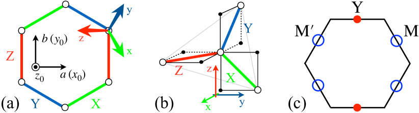
Figure 1: (a) The nearest-neighbor Ru-Ru $\{{\rm X,Y,Z}\}$ bonds, crystallographic $\{x_{0},y_{0},z_{0}\}$ and cubic $\{\rm x,y,z\}$ axes, and principal in-plane $a(b)$ directions. (b) Cubic axes and idealized Ru-Cl bonds. (c) Brillouin zone with the ordering vectors of the zigzag phase Y, M, and M’.

The postulated minimal microscopic two-dimensional (2D) spin model of $\alpha$-RuCl₃ is the $K$–$J$–$\Gamma$–$\Gamma^{\prime}$–$J_{3}$ or generalized Kitaev-Heisenberg model kee16 ; winter16 ; okamoto19 ,

$$\hat{\cal H}=\hat{\cal H}_{1}+\hat{\cal H}_{3}=\sum_{\langle ij\rangle}\mathbf{S}^{\rm T}_{i}\hat{\bm{J}}_{ij}\mathbf{S}_{j}+J_{3}\sum_{\langle ij\rangle_{3}}\mathbf{S}_{i}\cdot\mathbf{S}_{j}\,,$$ (1)

where ${\bf S}_{i}^{\rm T}=\left(S_{i}^{x},S_{i}^{y},S_{i}^{z}\right)$, the third-neighbor exchange is assumed isotropic, and $\hat{\bm{J}}_{ij}$ is the nearest-neighbor bond-dependent exchange matrix. Since the spin-rotational symmetries in the anisotropic-exchange Hamiltonians are, generally, absent, the allowed matrix elements of $\hat{\bm{J}}_{ij}$ are determined solely by the symmetry of the lattice RauGp .

For $\alpha$-RuCl₃ and related materials WinterReview , the conventional choice of the Cartesian reference frames for the spin projections are the so-called cubic axes, see Fig. 1. They correspond to an idealized undistorted octahedral environment of Ru³⁺ and are not coincidental with the plane of magnetic ions, the point that is often lost on a non-expert or a casual reader. These axes are natural within the orbital model considerations WinterReview , leading to a parametrization of the exchange matrix $\hat{\bm{J}}_{ij}$ that converts the nearest-neighbor part of the model (1) into

$$\mathcal{H}_{1}= \sum_{\langle ij\rangle_{\gamma}}\Big{[}J\mathbf{S}_{i}\cdot\mathbf{S}_{j}+KS^{\gamma}_{i}S^{\gamma}_{j}+\Gamma\left(S^{\alpha}_{i}S^{\beta}_{j}+S^{\beta}_{i}S^{\alpha}_{j}\right)$$

$$\ \ \ \ \ +\Gamma^{\prime}\left(S^{\gamma}_{i}S^{\alpha}_{j}+S^{\gamma}_{i}S^{\beta}_{j}+S^{\alpha}_{i}S^{\gamma}_{j}+S^{\beta}_{i}S^{\gamma}_{j}\right)\Big{]},$$ (2)

where $\langle ij\rangle_{\gamma}$ numerates the bonds $\gamma=\{{\rm X,Y,Z}\}$, with the triads of $\{\alpha,\beta,\gamma\}$ being $\{{\rm y,z,x}\}$ on the X bond, $\{{\rm z,x,y}\}$ on the Y bond, and $\{{\rm x,y,z}\}$ on the Z bond, respectively, see Fig. 1 for the cubic axes, crystallographic reference frame $\{x_{0},y_{0},z_{0}\}$, and other notations. We also note that the parametrization of the exchange matrix $\hat{\bm{J}}_{ij}$ that is used in (2) is a subject of some less-than-obvious transformations ChKh15 under relatively trivial symmetry operations discussed in Sec. IV.

A number of the $\{J,K,\Gamma,\Gamma^{\prime},J_{3}\}$ parameter sets have been proposed to describe $\alpha$-RuCl₃ using the first-principles methods winter16 ; kee16 ; gong17 ; li17 ; berlijn19 ; hozoi16 and phenomenological analyses wen17 ; winter17 ; suga18 ; moore18 ; orenstein18 ; gedik19 ; kim19 ; okamoto19 ; kaib19 ; nagler16 . We provide a compilation of them in Table 1 in the end of this Section and compare with the ranges advocated in the present study. The coupling that is believed to be the leading one is the (negative) Kitaev term, $K\!<\!0$. The off-diagonal $\Gamma\!>\!0$ term is also discussed as significant and potentially comparable to $|K|$, while the ferromagnetic exchange $J\!<\!0$ is believed to be subleading WinterReview . All three “main” parameters vary quite significantly between the studies, with the antiferromagnetic third-neighbor $J_{3}$ of the same order as $|J|$ also frequently invoked, and a small, predominantly negative $\Gamma^{\prime}$ included as being allowed by symmetry RauGp ; winter16 ; okamoto19 .

In the following, we use the first-principle guidance for $\alpha$-RuCl₃ winter16 and assume that $K\!<\!0$. We also use other restrictions from these works, such as some of the prevalent hierarchies of the couplings. However, we demonstrate that it is the currently available phenomenology that is powerful enough to significantly restrict and drastically revise the physically reasonable parameter space of the generalized KH model for $\alpha$-RuCl₃.

II.1 ESR and THz data

The electron spin resonance (ESR), terahertz (THz), and Raman spectroscopies have provided detailed information on the $\mathbf{q}\!=\!0$ magnetic excitations of $\alpha$-RuCl₃ and their field evolution in the fluctuating paramagnetic state Zvyagin17 ; kaib19 ; Wulferding19 . While a rich spectrum with multiple modes has been analyzed kaib19 , we focus on the field-dependence of the low-energy single-magnon mode F_footnote .

In Fig. 2, we show the data for this mode from the ESR (Ref. Zvyagin17 ) and THz (Ref. kaib19 ) studies for the in-plane field direction that is perpendicular to the Ru-Ru bond, referred to as the $a$-direction, for the field range from the critical field $H^{(a)}_{c}\!\approx\!6\text{T}$ to 35T. The data for the field along the $b$-direction are quite similar, suggesting nearly equal $g$-factors, the point also supported by the earlier studies hozoi16 ; Winter18 . We provide a fit of the data by

$$\varepsilon_{0}\!=\!h+a_{0}+a_{1}/h\,,$$ (3)

with $h\!=\!g\mu_{B}H$, $a_{0}\!=\!4.2$ meV, and $a_{1}\!=\!30$ meV², which is motivated by the high-field expansion of Eq. (4) below. Throughout this work, we use $g_{a}\!=\!g_{b}\!=\!2.5$, which is in accord with the previous estimates hozoi16 ; Winter18 ; Kubota15 .

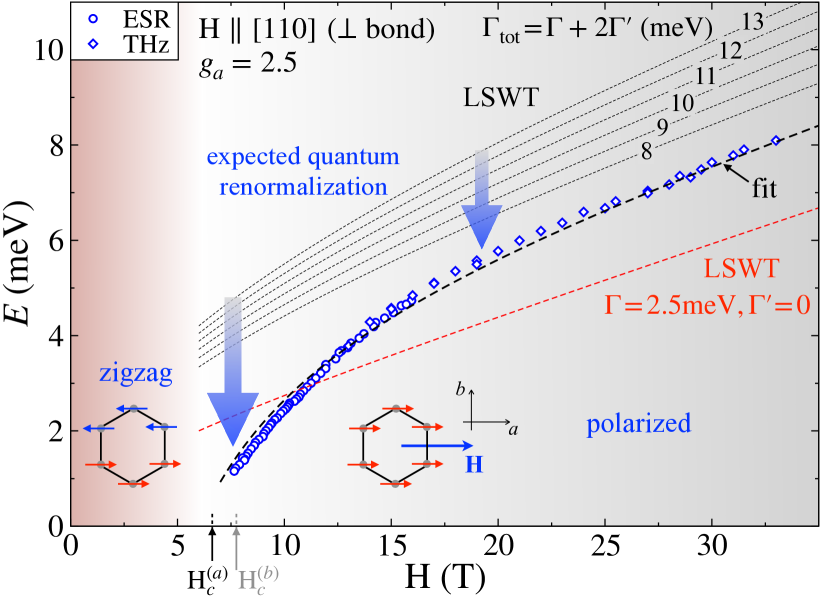
Figure 2: ESR Zvyagin17 and THz kaib19 data and their fit for the magnon energy gap, $\varepsilon_{0}$, at $\mathbf{q}\!=\!{\bf 0}$ vs field in the $a$-direction; LSWT results from Eq. (4) for representative $\Gamma_{\rm tot}$ from 8 meV to 13 meV and for $\Gamma\!=\!2.5$ meV winter17 for a comparison. Arrows indicate anticipated downward renormalization of the LSWT results by quantum fluctuations. Insets: sketches of the zigzag and polarized states and in-plane $a$ and $b$ directions.

Importantly, the linear spin-wave theory (LSWT) gives the $\mathbf{q}\!=\!0$ magnon energy that depends on a combination of only two parameters of the model (1), $\Gamma_{\rm tot}\!=\!\Gamma+2\Gamma^{\prime}$,

$$\varepsilon^{(0)}_{0}=\sqrt{h\big{(}h+3S\big{(}\Gamma+2\Gamma^{\prime}\big{)}\big{)}},$$ (4)

where $h\!=\!g\mu_{B}H$. This result is asymptotically exact in the $H\!\rightarrow\!\infty$ limit where fluctuations are suppressed. Expansion of (4) in $1/h$ yields the form used in (3).

In Fig. 2, we present LSWT results for several representative $\Gamma_{\rm tot}$ from 8 to 13 meV. The lowest LSWT line ($\Gamma\!=\!2.5$ meV) uses parameters that were successful in describing the low-field phenomenology of $\alpha$-RuCl₃ winter17 ; moore18 , but clearly fail to reproduce the high-field data, suggesting significantly larger $\Gamma_{\rm tot}$. The key point is that one should generally expect a downward renormalization of the LSWT spectrum due to quantum fluctuations winter17 ; tri09 , as is confirmed by a comparison with the exact diagonalization results of Ref. Winter18 in Sec. III.

Therefore, it is clear from Fig. 2 that $\Gamma_{\rm tot}$ cannot be less than $\approx\!8$ meV and it is also hard to justify it to be larger than $\approx\!13$ meV as this would imply unphysically large fluctuations in a strongly gapped high-field state. Thus, while the latter is not a precise constraint, there is a clear sense of both the lower and the upper bounds on the value of $\Gamma+2\Gamma^{\prime}$ from the ESR and THz data.

Qualitatively, fluctuations produce the downward shift of the spectrum due to repulsion of the one- and two-magnon states, which is expected to get stronger near the critical field, in agreement with Fig. 2 and with a discussion in Ref. kaib19 . We also note, that the observed single-magnon energy can be related to the “bare” LSWT result of Eq. (4) as $\varepsilon_{0}\!=\!\Lambda\varepsilon^{(0)}_{0}$, where $\Lambda$ is the field-dependent renormalization factor with the high-field behavior $\Lambda\!=\!1-O(h^{-1})$. Thus, while naively one can extract $\Gamma_{\rm tot}$ using expansion in Eq. (3) directly from the $a_{0}$ term, the fluctuation factor provides a significant correction to it that requires a self-consistent consideration.

As we show in Sec. III, the field-dependent renormalization factor can be approximated by the reduced ordered moment, $\Lambda\!=\!\langle S\rangle/S$, as follows from the self-consistent random-phase approximation (RPA) Tyablikov . According to it, fluctuation corrections to $\varepsilon^{(0)}_{0}$ at higher fields can still produce a substantial downward shift, suggesting the lower limit for $\Gamma_{\rm tot}$ to be $\gtrsim 9$ meV.

II.2 Critical fields

In $\alpha$-RuCl₃, the in-plane field induces a phase transition from the zigzag to a fluctuating paramagnetic state at a critical field about $7$T Winter18 ; Cao16 ; NaglerVojta18 , see Fig. 2. An additional transition at a lower field NaglerVojta18 has been identified with an interplane ordering Baltz19 ; Vojta3D and is unrelated to the key physics of $\alpha$-RuCl₃ discussed in this work footnote3D .

In the field-induced paramagnetic phase, magnon spectrum is gapped and the transition to the zigzag phase upon lowering the field corresponds to a softening of the spectrum. The gap closes at the ordering vectors associated with the zigzag structure, the face-centers of the Brillouin zone, see Fig. 1(c). For $H\!\parallel\!b$, the ordering vector of the single field-selected zigzag domain is Y, and for $H\!\parallel\!a$, the two domains have the ordering vectors at the M and M^′ points, respectively Sears17 ; orenstein18 ; Vojta3D .

In the paramagnetic phase spins are oriented along the field and the magnon spectrum can be obtained analytically, see Appendix A. The condition on the gap closing yields the critical fields for $H\!\parallel\!a$ and $H\!\parallel\!b$, see also footnote_Hc

$$h_{c}^{(a)} =J+3J_{3}+\frac{1}{12}\big{(}5K-5\Gamma-16\Gamma^{\prime}\big{)}$$ (5)

$$+\frac{1}{12}\sqrt{\big{(}K+5\Gamma+4\Gamma^{\prime}\big{)}^{2}+24\big{(}K-\Gamma+\Gamma^{\prime}\big{)}^{2}},$$

$$h_{c}^{(b)} =J+3J_{3}+\frac{1}{4}\big{(}2K-\Gamma-6\Gamma^{\prime}\big{)}$$ (6)

$$+\frac{1}{12}\sqrt{\big{(}2K+7\Gamma+2\Gamma^{\prime}\big{)}^{2}+32\big{(}K-\Gamma+\Gamma^{\prime}\big{)}^{2}},$$

where $h_{c}^{(\alpha)}\!=\!g_{\alpha}\mu_{B}H_{c}^{(\alpha)}$. An important feature of these results is that the difference of the critical fields in (5) and (6) appears to be a function of only three anisotropic terms of the model: $K,\Gamma$, and $\Gamma^{\prime}$. As is discussed above, we assume the $g$-factors in the two principal directions to be the same, so $\Delta h_{c}\!=\!g\Delta H_{c}$, with $\Delta H_{c}\!=\!H_{c}^{(b)}\!-\!H_{c}^{(a)}$. This feature is key to the constraints proposed below.

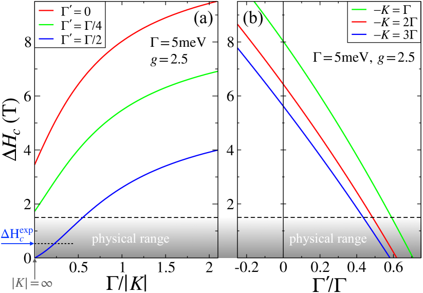
Figure 3: (a) The difference of the critical fields from Eqs. (5) and (6), $\Delta H_{c}\!=\!H_{c}^{(b)}\!-\!H_{c}^{(a)}$, vs $\Gamma/|K|$ for representative values of $\Gamma^{\prime}/\Gamma$ and $\Gamma\!=\!5$ meV. (b) $\Delta H_{c}$ vs $\Gamma^{\prime}/\Gamma$ for representative ratios of $K/\Gamma$. The physical range for $\Delta H_{c}$ is $<\!1.5$T, see text; the experimental value is $\Delta H_{c}^{\rm exp}\!=\!0.6$T NaglerVojta18 . The physical range requires significant $\Gamma^{\prime}\!\sim\!\Gamma/2\!>\!0$.

Before we discuss them in more detail, we note that, experimentally, the critical fields in $\alpha$-RuCl₃ for $a$- and $b$-directions are nearly identical Zvyagin17 ; NaglerVojta18 . While small $\Delta H_{c}$ seems to be a minor point, it is virtually impossible to reproduce from Eqs. (5) and (6) without a sizable $\Gamma^{\prime}$, the difficulty also clearly encountered in Ref. NaglerVojta18 that used a model with $\Gamma^{\prime}\!=\!0$.

We demonstrate this by Fig. 3(a) showing $\Delta H_{c}$ vs $\Gamma/|K|$ for several values of $\Gamma^{\prime}/\Gamma$ and for a representative value of $\Gamma\!=\!5$ meV, see Table 1. The highlighted physical range for $\Delta H_{c}$ is chosen as $<\!1.5$T to account for possible difference of the $g$-factors, while the experimental value is $\Delta H_{c}^{\rm exp}\!=\!0.6$T NaglerVojta18 . It is clear from Fig. 3, that even at $|K|\!\rightarrow\!\infty$ the asymptotic value of $\Delta H_{c}$ for $\Gamma^{\prime}\!=\!0$ is well above the physical range and a positive $\Gamma^{\prime}\!\gtrsim\!\Gamma/2$ is needed to reach it. The same effect is illustrated in Fig. 3(b), with $\Delta H_{c}$ plotted vs $\Gamma^{\prime}/\Gamma$ for three representative ratios of $K/\Gamma$. Again, a model without a significant positive $\Gamma^{\prime}$ cannot reproduce observed small difference between the critical fields.

Superficially, a large positive $\Gamma^{\prime}$ contradicts first-principles results for $\alpha$-RuCl₃ winter16 ; kee16 ; berlijn19 . However, as we discussed in Sec. I, our model implicitly incorporates further-neighbor terms into fewer effective parameters, with a phenomenology dictating physical answer. This result is also in accord with the ESR/THz constraints that require large $\Gamma\!+\!2\Gamma^{\prime}$. Having substantial $\Gamma^{\prime}\!\sim\!\Gamma/2$ removes the need for the unphysically large $\Gamma$ in explaining some of the other $\alpha$-RuCl₃ phenomenologies wen17 ; kim19 ; okamoto19 .

One concern is the potential effect of quantum fluctuation corrections on the LSWT results for the critical fields in Eqs. (5) and (6). However, such corrections are unlikely to affect the smallness of their difference, $\Delta H_{c}\!\ll\!H_{c}^{(a/b)}$, and the arguments on a sizable $\Gamma^{\prime}$ that follow from it. Moreover, the self-consistent mean-field RPA approach advocated in Sec. III predicts no quantum effects on the critical fields. Near the transition, Zeeman energy of the fluctuating spin polarization, $(H-H_{c})\langle S\rangle$, competes with the gap that is reduced by quantum fluctuations, $\Lambda\Delta^{(0)}$, where $\Lambda\!=\!\langle S\rangle/S$ as suggested above Tyablikov . Then, the condition on closing of the gap is the same as within the LSWT, in which bare Zeeman energy, $(H-H_{c})S$, competes with the bare gap, $\Delta^{(0)}$. Thus, the critical field is unchanged by the fluctuations. While this is a mean-field argument, it points to suppressed quantum effects on the critical fields.

II.3 Empirical constraints, I

As is discussed above, for the model (1) of $\alpha$-RuCl₃ there are bounds on $\Gamma_{\rm tot}\!=\!\Gamma+2\Gamma^{\prime}$ and on $\Delta H_{c}$. Moreover, $\Delta H_{c}$ depends only on three parameters of the model: $\Delta H_{c}(K,\Gamma,\Gamma^{\prime})$. Thus, if one would be able to fix exactly both $\Gamma_{\rm tot}$ and $\Delta H_{c}$, this would restrict the 3D parameter subspace of $\{K,\Gamma,\Gamma^{\prime}\}$ to a 1D curve.

To get an insight into the resulting constraints, we show projections of such curves onto the $K$–$\Gamma$ plane in Figure 4 for four sets of $\{\Gamma_{\rm tot},\Delta H_{c}\}$ with $\Gamma_{\rm tot}\!=\!9$ meV and 13 meV and $\Delta H_{c}\!=\!0.5$T and 1.5T. Obviously, the entire range of $\Gamma_{\rm tot}$ from 9 meV to 13 meV and of $\Delta H_{c}$ from 0.5T to 1.5T are confined between these curves, shown by the shaded area. This range of $\Gamma_{\rm tot}$ is bounded by the ESR/THz as discussed above. Instead of fixing $\Delta H_{c}$ to its experimental value of 0.6T NaglerVojta18 , we allow for an additional range from 0.5T to 1.5T to account for small differences in the $g$-factors and for the residual quantum corrections to $H_{c}^{(a)}$ and $H_{c}^{(b)}$in Eqs. (5) and (6).

It is clear from Fig. 4, that the values of $\Gamma$ are strongly constrained already at this stage, while there is no upper limit on $|K|$. An expression for $K(\Gamma,\Gamma_{\rm tot},\Delta H_{c})$ vs $\Gamma$ indeed displays an unbounded asymptotic form $K\!\sim\!1/(\Gamma-\Gamma_{\rm max})$ with $\Gamma_{\rm max}\!=\!\Gamma_{\rm tot}/2+5\Delta h_{c}$. Figure 4 shows such $\Gamma_{\rm max}$ by the dashed line for the upper-boundary values of $\Gamma_{\rm tot}\!=\!13$ meV and $\Delta H_{c}\!=\!1.5$T.

The main message of Fig. 4 is that $\Gamma$ for the model (1) of $\alpha$-RuCl₃ is constrained from both below and above mainly by the bounds on $\Gamma_{\rm tot}$ from the ESR/THz gap and to a lesser extent by the variation of allowed $\Delta H_{c}$, while $K$ is only restricted by the choice of $K\!<\!0$. However, Kitaev term also has physical constraints, see Table 1, as we highlight in Fig. 4, which should lead to even tighter bounds on the possible ranges of $\Gamma$. Overall, the “typical” value of $\Gamma$ appears to be $\sim\!\Gamma_{\rm tot}/2$, and $\Gamma^{\prime}\!\sim\!\Gamma/2$.

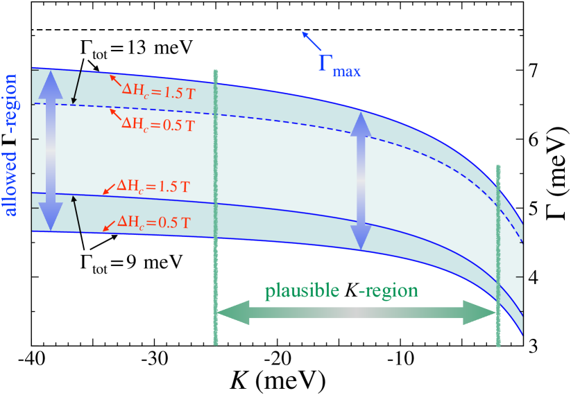
Figure 4: The $K$–$\Gamma$ projection of the parameter range restricted by two constraints: 9 meV$<\!\Gamma+2\Gamma^{\prime}\!<\!13$ meV and 0.5T$<\!\Delta H_{c}\!<\!1.5$T (shaded area). $\Gamma_{\rm max}$ (dashed line) is the asymptotic value of the upper boundary of the shaded region, $\{\Gamma_{\rm tot},\Delta H_{c}\}\!=\!\{13\,{\rm meV},1.5\,{\rm T}\}$, for $|K|\!\rightarrow\!\infty$. Plausible region for $K$ suggested by the prior estimates, Table 1, is indicated.

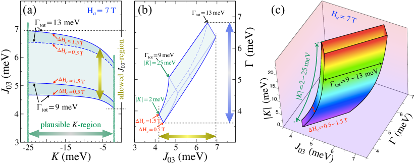
Figure 5: (a) The $K$–$J_{03}$ and (b) the $J_{03}$–$\Gamma$ projections of the parameter space allowed by three constraints: $9\!<\!\Gamma_{\rm tot}\!<\!13$ meV, $0.5\!<\!\Delta H_{c}\!<\!1.5$T, and $H_{c}^{(a)}\!=\!7$T. These criteria strongly bind $\Gamma$ and $J_{03}$, see (b). The $K$–$J_{03}$ projection in (a) is similar to the $K$–$\Gamma$ projection in Fig. 4, with the upper and lower limits on $J_{03}$ and plausible boundaries on the Kitaev term $K$ indicated. (c) The 3D $J_{03}$–$\Gamma$–$K$ subspace of the allowed parameters, with the extent of $\Gamma_{\rm tot}$ giving the length, $\Delta H_{c}$ determining the width, and $K$ restricting the height of the 3D region. Projections of this 3D object yield Figs. 4, 5(a) and 5(b).

There is an important feature of the critical fields $H_{c}^{(a)}$ and $H_{c}^{(b)}$ given by Eqs. (5) and (6). They both depend on the Heisenberg exchanges only via a linear combination

$$J_{03}\equiv J+3J_{3},$$ (7)

which makes $J_{03}$ a natural variable in the discussion of the empirical constraints. Quantitatively, this dependence is also very strong. Using $g\!=\!2.5$, a relatively small change of $J_{3}$ by 0.3 meV modifies $H_{c}$ by about 6T. Incidentally, this also mitigates concerns about quantum effects on experimental values of the critical fields compared to the theoretical ones, as a small adjustment of $J_{3}$ in the latter is sufficient to match the former.

Thus, for the purpose of considering critical fields, the 5D parameter space of the model (1) of $\alpha$-RuCl₃ is effectively reduced to a 4D subspace by using $J_{03}$ from Eq. (7): $H_{c}^{(\alpha)}\!=\!H_{c}^{(\alpha)}(K,\Gamma,\Gamma^{\prime},J_{03})$. Using the same bounds on $\Gamma_{\rm tot}$ and $\Delta H_{c}$ as in Fig. 4 and experimental value of $H_{c,{\rm exp}}^{(a)}\!=\!7$T NaglerVojta18 allows us to put constraints on $J_{03}$ in a similar manner to that of the $\Gamma$-term.

As one can see from Figure 5(a), the $K$–$J_{03}$ projection of the parameter range restricted by these constraints shows the same characteristics as the $K$–$\Gamma$ projection in Fig. 4. That is, $J_{03}$ is constrained from below and above, while $K$ is only semi-bounded. In addition, the “plausible range” of $2\!<\!|K|\!<\!25$ meV, see Table 1, further restricts $J_{03}$ within the “typical” values that are very similar to that of $\Gamma$, $J_{03}\!\sim\!\Gamma_{\rm tot}/2$. We note that these results are rather insensitive to the variations of $H_{c,{\rm exp}}^{(a)}$, easily so within the limits of $\pm$2T, as they can be effectively absorbed into small changes of $J_{03}$ of order $\sim\!0.1$ meV.

Altogether, constraints on the parameters of the model (1) of $\alpha$-RuCl₃ discussed so far have resulted in strong bounds on $\Gamma$ and $J_{03}$. This is demonstrated explicitly in Figure 5(b), which shows a $J_{03}$–$\Gamma$ projection of the allowed parameter ranges that are restricted by the same limits as in Figs. 4 and 5(a), dictated by the ESR/THz gap, variation of $\Delta H_{c}$, and fixed $H_{c,{\rm exp}}^{(a)}\!=\!7$T. In this Figure, the narrow width of the projection is mostly controlled by $\Delta H_{c}$, while the length is due to the limits on $\Gamma_{\rm tot}$ and $K$. In Fig. 5(b), we explicitly limited $K$ to the “plausible range” of 2 meV$<\!|K|\!<$25 meV.

Lastly, all three projections of Figs. 4, 5(a), and 5(b) are summarized as a 3D shape in Figure 5(c), which makes it explicit that the allowed regions illustrated in each Figure correspond to a projection of this three-dimensional object onto a respective plane. The aforementioned correlations between different parameters also become clearer, with the upper and lower bounds on $\Gamma_{\rm tot}$ providing the ranges for $\Gamma$ and $J_{03}$, while the difference of the critical fields $\Delta H_{c}$ is giving a narrow width of the allowed 3D parameter space. However, Kitaev term remains unbounded and so do the Heisenberg exchanges $J$ and $J_{3}$, as we have only restricted their combination. Therefore, more empirical constraints are needed.

II.4 Empirical constraints, II

To establish further constraints for the model (1) of $\alpha$-RuCl₃, we employ two additional “soft” criteria motivated by several experimental results. Below we discuss the range of the out-of-plane tilt angle of spins in the zigzag state and an overall upper limit on the energy bandwidth of the observed magnetic intensity.

First of the “soft” criteria is the experimentally observed tilt of the spins away from the $ab$-plane in zero-field zigzag ground state of $\alpha$-RuCl₃, see inset in Fig. 6. This effect has been discussed in Refs. ChKh15 ; Chaloupka16 , with the tilt occurring due to anisotropic terms and the angle in the classical limit given by

$$\tan 2\alpha=4\sqrt{2}\,\frac{1+r}{7r-2},\ \ \ r=-\frac{\Gamma}{K+\Gamma^{\prime}}.$$ (8)

It has also been analyzed by the neutron diffraction, muon spin relaxation, and resonant elastic x-ray scattering Cao16 ; Tanaka18 ; kim19 , with the best fits giving the tilt angle around $\alpha\!\approx\!35^{\circ}$, see Fig. 6. By comparing to exact diagonalization, it was shown in Ref. Chaloupka16 that quantum corrections can modify the classical value of $\alpha$ by about 5^∘. Furthermore, there may be a difference between the calculated direction of the pseudospin in (8) and the experimentally measured direction of the magnetic moment, see Ref. Chaloupka16 . To account for these effects, we take a generous range of $25^{\circ}\!<\!\alpha\!<\!45^{\circ}$ as our criterion instead of fixing the tilt angle to a particular value, see also Appendix C.

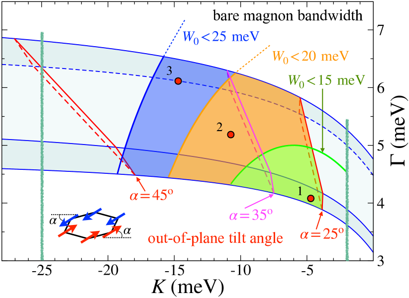
Figure 6: Same as Fig. 4 with constraints on the tilt angle $\alpha$ (shown in the inset) and on magnetic intensity width $W_{0}$, see text. Dots are representative parameter sets from Sec. II E.

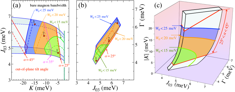
Figure 7: Same as Fig. 5 with constraints on the tilt angle $\alpha$, magnetic intensity width $W_{0}$ (“realistic” $\lesssim\!15$ meV, “generous” $\lesssim\!20$ meV, and “outrageous” $\lesssim\!25$ meV), and zigzag ground state, see text. Dots are parameter sets from Sec. II E.

Figures 6 and 7 show the effect of this constraint on various projections of the allowed parameter space. We note that the classical expression (8) can be solved analytically for small $\alpha$, giving $|K|\!\approx\!0.9\Gamma$ for $\Gamma^{\prime}\!=\!\Gamma/2$, which agrees closely with the $\alpha\!=\!25^{\circ}$ boundary for the $K\!-\!\Gamma$ plane in Fig. 6, obtained numerically. One can see that the most important effect of the constraint on the tilt angle is the lower boundary on $|K|$. This is physically meaningful as the tilt can only occur due to the non-zero anisotropic terms, $K$, $\Gamma$, and $\Gamma^{\prime}$, see also Ref. kim19 .

Our second criterion is the upper limit on the energy bandwidth of the magnetic intensity observed by the neutron and Raman scattering nagler16 ; Banerjee17 ; kaib19 ; Wulferding19 , which sets a logical upper bounds on the model parameters. In zero field, the bulk of the magnetic spectral weight is found below $\lesssim\!8$ meV, with extrapolations of the upper limit of the measurable signal extending to at most 15–20 meV.

We make two general assumptions. First, the width of the detectable spectrum intensity is exhausted by one- and two-magnon excitations, which is true for the well-ordered phases such as the zero-field zigzag state of $\alpha$-RuCl₃. Even in the case of the pure Kitaev model, the basis of spin-flips is still complete, thus suggesting that this measure should provide a reasonable estimate of the bandwidth of any type of excitations. This yields the spectrum intensity width as $2W_{0}$, where $W_{0}$ is the “bare” LSWT single-magnon bandwidth. Second, as is discussed above and in Sec. III, there is a quantum renormalization factor for the spectrum that can be approximated within the RPA Tyablikov by a reduced ordered moment, $\Lambda\!=\!\langle S\rangle/S$, thus narrowing the effective extent of the one- and two-magnon spectrum to $\approx\!2\Lambda W_{0}$.

The experimental estimates of the reduced ordered moment vary around $\Lambda\!\approx\!0.5$ Coldea15 ; Cao16 , with the our LSWT calculations in Sec. III suggesting a factor of 0.44. Taken together, the “bare” LSWT one-magnon bandwidth $W_{0}$ itself is roughly equivalent to an effective extent of the detectable magnetic intensity. This consideration, together with the experimental limits discussed above, create the basis for our criterion. In the spirit of keeping this criterion “soft”, we present several versions of the constraint for $W_{0}$: “realistic” $\lesssim\!15$ meV, “generous” $\lesssim\!20$ meV, and “outrageous” $\lesssim\!25$ meV cutoff values.

We also combine the constraint on $W_{0}$ with the verification that the zero-field ground state is indeed a zigzag state for all parameter choices and that no intermediate phases occur between $H\!=\!0$ and $H\!=\!H_{c}$. For the first, we use the Luttinger-Tisza (LT) approach LT , and for the second we inspect possible spectrum instabilities within the LSWT. This combination of the $W_{0}$ and zigzag criteria is essential as they are less stringent separately.

Figures 6 and 7 show the results of these constraints on different projections of the allowed parameter space. The constraints on $W_{0}$ and zigzag are found numerically from the LSWT and LT, but for the boundaries shown in Figs. 6 and 7 we use a fit W0_fit that closely approximates them. One can see that the most important effect of these constraints is the upper boundary on $|K|$ and a tighter bound on $\Gamma$ and $J_{03}$ for the “realistic” $W_{0}$ limit.

For the $K$–$\Gamma$–$J_{03}$ subspace exhibited in Figs. 6 and 7, the boundary of the zigzag with an incommensurate phase occurs at both smaller and larger $|K|$. For the smaller $|K|$, it is superseded by the lower bound on the tilt angle $\alpha\!>\!25^{\circ}$. While the bandwidth limit does constrain the value of $|K|$ from above by itself, the combined effect with the zigzag requirement is considerably stronger. Thus, the boundary of each color-coded shape in Figs. 6 and 7 for large values of $|K|$ is also a boundary to an incommensurate state. This is in a broad agreement with Ref. NaglerVojta18 , where larger $|K|/|J|$ led to phases different from the zigzag, see also Appendix C.

In Figure 8 we show a projection of the allowed parameter space onto the $\Gamma$–$\Gamma^{\prime}$ plane, which quantitatively confirms our earlier assertion that $\Gamma^{\prime}$ should be large and positive. The boundaries of the $\Gamma$–$\Gamma^{\prime}$ region are set by the ESR/THz bounds on $\Gamma_{\rm tot}\!=\!\Gamma+2\Gamma^{\prime}$, with $\Gamma^{\text{min}}_{\rm tot}\!=\!9$ meV and $\Gamma^{\text{max}}_{\rm tot}\!=\!13$ meV, as well as by the lower boundary on the tilt angle $\alpha\!=\!25^{\circ}$ from above and on the bandwidth $W_{0}$ and zigzag from below. The latter are more stringent than the restrictions from $\Delta H_{c}$ (not shown), that were advocated earlier. One can also observe that, overall, $\Gamma^{\prime}$ is strongly tied to $\Gamma$, which, in turn, is $\approx\!\Gamma_{\rm tot}/2$.

Figure 8: The $\Gamma$–$\Gamma^{\prime}$ projection of the parameter regions with all the constraints. Dots are parameter sets from Sec. II E.

Lastly, we present the $J$–$J_{3}$ projection in Fig. 9. According to our prior discussion, a combination of $J$ and $J_{3}$, termed $J_{03}$ in (7), is restricted and correlates narrowly with $\Gamma$, while, individually, these exchanges are unbounded. In Figure 9, their allowed region is confined between parallel lines that are defined by the lower and upper limits of $J_{03}$ from Fig. 7 and Eq. (7).

The zigzag ground state is stabilized by the larger values of $|J|$ and $J_{3}$, in agreement with the previous work that pointed out that trend Kimchi11 . One can see that the constraints on the spectral width $W_{0}$ and on the zigzag state are responsible for the majority of the $J$ and $J_{3}$ boundaries for both “realistic” and “generous” $W_{0}$, while the parameter region for the “outrageous” (25 meV) choice of $W_{0}$ also encounters other boundaries.

These additional constraints are imposed by the ab initio results. As one can see in Table 1, the ab initio methods set a rather strict hierarchy on the parameters of the model (1) of $\alpha$-RuCl₃: $K$ and $\Gamma$ are dominant, while the rest of the terms are subleading. This produces an additional constraint, $|J|,J_{3}\!<\!|K|,\Gamma$, that limits $|J|$ and $J_{3}$ from above. Since $\Gamma$ is bounded by the ESR/THz constraints on $\Gamma_{\rm tot}$, this ab initio-guided constraint together with the definition of $J_{03}$ in Eq. (7) lead to close approximations for the upper limits on $|J|$ and $J_{3}$ in terms of $\Gamma^{\text{max}}_{\rm tot}$ shown in Fig. 9. In addition, one of the boundaries in Fig. 9 is due to an explicit constraint $|J|\!<\!\Gamma^{\text{max}}$.

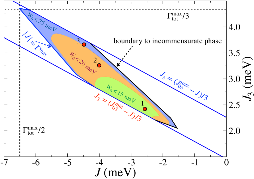
Figure 9: The $J$–$J_{3}$ projection of the parameter space, subject to all constraints discussed in text. Boundaries to an incommensurate phase are from the ab initio-guided constraints $|J|\!<\!\Gamma^{\text{max}}\!=\!6.5$ meV, $|J|\!\lesssim\!\Gamma_{\rm tot}^{\text{max}}/2$, and $J_{3}\!\lesssim\!\Gamma_{\rm tot}^{\text{max}}/3$, see text. Dots are parameter sets from Sec. II E.

II.5 Summary

Altogether, we have provided a series of empirical constraints of varying rigidity on the parameters of the model (1) for $\alpha$-RuCl₃, with an overall qualitative, if somewhat crude take-home message. Most of the terms of the model are related to the same parameter, $\Gamma_{\rm tot}$, which is bounded by the ESR/THz constraints. Specifically, $\Gamma\!\approx\!J_{03}\!\approx\!\Gamma_{\rm tot}/2$ and $\Gamma^{\prime}\!\approx\!\Gamma/2$. The leading parameter is less constrained, with the ratio $|K|/\Gamma\!\approx\!1.0-3.0$, and $J$ and $J_{3}$ require finer adjustments to the experimental value of $H_{c}^{(a)}$. Empirically, $|J|/\Gamma\!\approx\!J_{3}/\Gamma\!\approx\!0.5-0.75$.

These constraints and limits are represented in our Figs. 6, 7, 8, and 9. In these Figures, we also show the representative points from each of the three regions bounded by the different constraint on the bandwidth $W_{0}$, with the following $(K,\Gamma,\Gamma^{\prime},J,J_{3})$ coordinates and the corresponding values of $\{\Gamma_{\rm tot},J_{03}\}$, all in meV:

	$(K,$	$\Gamma,$	$\Gamma^{\prime},$	$J,$	$J_{3})\$	$\{\Gamma_{\rm tot},$	$J_{03}\}$
Point 1:	(-4.8,	4.08,	2.5,	-2.56,	2.42)	$\{9.08,$	$4.70\}$
Point 2:	(-10.8,	5.2,	2.9,	-4.0,	3.26)	$\{11.0,$	$5.78\}$
Point 3:	(-14.8,	6.12,	3.28,	-4.48,	3.66)	$\{12.7,$	$6.50\}$

Some properties of these parameter sets, such as linear spin-wave spectrum, magnetization, Néel temperature, and critical fields, are presented in Sec. III.

II.6 Compilation of parameters

Reference	Method	$K$	$\Gamma$	$\Gamma^{\prime}$	$J$	$J_{3}$	$\Gamma\!+\!2\Gamma^{\prime}$	$J\!+\!3J_{3}$
Banerjee et al. nagler16	LSWT, INS fit	+7.0			-4.6			-4.6
Kim et al. kee16	DFT+$t/U$, $P3$	-6.55	5.25	-0.95	-1.53		3.35	-1.53
	DFT+SOC+$t/U$	-8.21	4.16	-0.93	-0.97		2.3	-0.97
	same+fixed lattice	-3.55	7.08	-0.54	-2.76		6.01	-2.76
	same+$U$+zigzag	+4.6	6.42	-0.04	-3.5		6.34	-3.5
Winter et al. winter16	DFT+ED, $C2$	-6.67	6.6	-0.87	-1.67	2.8	4.87	6.73
	same, $P3$	+7.6	8.4	+0.2	-5.5	2.3	8.8	+1.4
Yadav et al. hozoi16	Quantum chemistry	-5.6	-0.87		+1.2		-0.87	+1.2
Ran et al. wen17	LSWT, INS fit	-6.8	9.5				9.5
	DFT+$t/U$, $U\!=\!2.5$eV	-14.43	6.43		-2.23	2.07	6.43	+3.97
Hou et al. gong17	same, $U\!=\!3.0$eV	-12.23	4.83		-1.93	1.6	4.83	+2.87
	same, $U\!=\!3.5$eV	-10.67	3.8		-1.73	1.27	3.8	+2.07
Wang et al. li17	DFT+$t/U$, $P3$	-10.9	6.1		-0.3	0.03	6.1	-0.21
	same, $C2$	-5.5	7.6		+0.1	0.1	7.6	+0.4
Winter et al. winter17	Ab initio+INS fit	-5.0	2.5		-0.5	0.5	2.5	+1.0
Suzuki et al. suga18	ED, $C_{p}$ fit	-24.41	5.25	-0.95	-1.53		3.35	-1.53
Cookmeyer​ et​ al. moore18	thermal Hall fit	-5.0	2.5		-0.5	0.11	2.5	-0.16
Wu et al. orenstein18	LSWT, THz fit	-2.8	2.4		-0.35	0.34	2.4	+0.67
Ozel et al. gedik19	same, $K\!>\!0$	+1.15	2.92	+1.27	-0.95		5.45	-0.95
	same, $K\!<\!0$	-3.5	2.35		+0.46		2.35	+0.46
Eichstaedt​ et​ al. berlijn19	DFT+Wannier+$t/U$	-14.3	9.8	-2.23	-1.4	0.97	5.33	+1.5
Sahasrabudhe​ et​ al.kaib19	ED, Raman fit	-10.0	3.75		-0.75	0.75	3.75	1.5
Sears et al. kim19	Magnetization fit	-10.0	10.6	-0.9	-2.7		8.8	-2.7
Laurell et al. okamoto19	ED, $C_{p}$ fit	-15.1	10.1	-0.12	-1.3	0.9	9.86	+1.4
This work	“realistic” range	[-11,-3.8]	[3.9,5.0]	[2.2,3.1]	[-4.1,-2.1]	[2.3,3.1]	[9.0,11.4]	[4.4,5.7]
	point 1	-4.8	4.08	2.5	-2.56	2.42	9.08	4.7
	point 2	-10.8	5.2	2.9	-4.0	3.26	11.0	5.78
	point 3	-14.8	6.12	3.28	-4.48	3.66	12.7	6.5

Table 1: The representative sets of parameters of the generalized KH model (1) for $\alpha$-RuCl₃ (in meV). The values that come close to the ranges proposed in this work are highlighted in bold. The common acronyms include linear spin-wave theory (LSWT), density-functional theory (DFT), spin-orbit coupling (SOC), inelastic neutron scattering (INS), exact diagonalization (ED), and terahertz spectroscopy (THz); structures of $P3$ and $C2$ symmetry are referred to as “$P3$” and “$C2$” for brevity.

Our Table 1 provides a representative compilation of the parameters of the model (1) that were proposed to describe $\alpha$-RuCl₃ using the first-principles methods winter16 ; kee16 ; gong17 ; li17 ; berlijn19 ; hozoi16 and phenomenological analyses wen17 ; winter17 ; suga18 ; moore18 ; orenstein18 ; gedik19 ; kim19 ; okamoto19 ; kaib19 ; nagler16 , with the first column providing the reference and the second abbreviating the details of the used approach. In cases when the proposed model description did not retain the $C_{3}$ symmetry of the ideal lattice structure, we used the bond-averaged values of the exchange parameters.

In Table 1, we also present our results for the ranges of individual parameters for the “realistic” cutoff on $W_{0}$ and for the representative Point 1,2,3 sets described above. We note again, that the parameters are correlated, with representative parameter sets illustrating these correlations. For instance, larger $\Gamma$ requires larger values of $\Gamma^{\prime}$, $|J|$, etc. In that sense, the parameter ranges do not do full justice to the constraints that we advocate, as the actual 5-dimensional constrained region is much narrower.

The listed values for each parameter are highlighted in bold in case they fall within or come close to our advocated “realistic” parameter range. Although one can see quite a few “hits” in case of $K$, these may be mostly attributed to an extensive random shooting.

There are two particularly notable differences of our results from the prior studies. First, is a significant and positive $\Gamma^{\prime}$, which is either completely absent in the previous considerations or is small and negative. In Section II, we have discussed extensively and made our case for the necessity of a significant $\Gamma^{\prime}\!>\!0$ in the effective model description (1) of $\alpha$-RuCl₃.

Second, are the “cumulative” parameters $\Gamma_{\rm tot}\!=\!\Gamma\!+\!2\Gamma^{\prime}$ and $J_{03}\!=\!J\!+\!3J_{3}$ in the last two columns of Table 1. For the case of $\Gamma_{\rm tot}$, there are a few studies providing comparable values, in which there is an attempt to describe phenomenology that is similar to ours, but without positive $\Gamma^{\prime}$. These attempts can be seen as trying to compensate for the lack of $\Gamma^{\prime}$ by cranking up $\Gamma$ kim19 ; okamoto19 . For $J_{03}$, it appears that previous works have, generally, underappreciated the importance of the mutual correlation of $J$ and $J_{3}$, leading to a nearly random distribution of their values. As is discussed above, this work underscores the phenomenological constraints on both $\Gamma_{\rm tot}$ and $J_{03}$ and the associated strong mutual bounds on $\Gamma$, $\Gamma^{\prime}$, and $J_{03}$, see Figs. 7 and 8.

Lastly, as is emphasized in Sec. I and Sec. II, the results of our work may differ from the prior analyses in Table 1 because we consider phenomenology of an effective model as opposed to the first-principles methods, and we also extract bare parameters that are typically larger than the ones reduced by quantum fluctuations.

III Quantum effects

In this section, we present the RPA results for the spectrum renormalization in the paramagnetic phase and demonstrate their close agreement with the ESR and THz data. As is shown above, the $\alpha$-RuCl₃ model has strong anisotropic-exchange interactions. They should inevitably lead to significant nonlinear quantum effects in the magnon spectra due to substantial three-particle interactions. Below, we calculate the damping of magnons due to associated decays and consider their effect in the spectrum and the dynamical structure factor.

III.1 Quantum fluctuations

Figure 10: The ED results for the magnon spectrum at $\mathbf{q}\!=\!0$ as a function of magnetic field for two principal directions (intensity plot), reproduced from Ref. Winter18 . Results for the single-magnon branch by LSWT, Eq. (4), (dashed line) and by the RPA (solid line) for the parameter set from Ref. Winter18 .

The self-consistent RPA approach is based on the mean-field decoupling of the equations of motion for the spin Green’s functions Tyablikov ; Plakida . It provides an approximate, yet effective, way of accounting for the downward spectrum renormalization by quantum fluctuations. For $S\!=\!1/2$, the result is particularly simple Tyablikov ; Plakida

$$\widetilde{\varepsilon}_{\mathbf{k}}=\Lambda\varepsilon_{\mathbf{k}},\quad\Lambda=\langle S\rangle/S,$$ (9)

where $\langle S\rangle$ is the average on-site magnetization reduced by quantum fluctuations, $\varepsilon_{\mathbf{k}}$ is the LSWT magnon energy, and $\widetilde{\varepsilon}_{\mathbf{k}}$ is the renormalized energy.

One can justify this approximation using unbiased numerical methods. In Figure 10, we provide a comparison of the RPA results with the ED calculations for the magnon energy spectrum at ${\bf q}\!=\!0$ in the paramagnetic phase vs field for two field orientations. The ED data are from Ref. Winter18 for the parameter set $K\!=\!-5$ meV, $\Gamma\!=\!2.5$ meV, $\Gamma^{\prime}\!=\!0$, and $J_{3}\!=\!-J\!=\!0.5$ meV, which has also been used in Refs. winter17 ; moore18 for different phenomenologies of $\alpha$-RuCl₃. One can see that RPA provides a significant improvement over the LSWT results and yields a good agreement with the numerics.

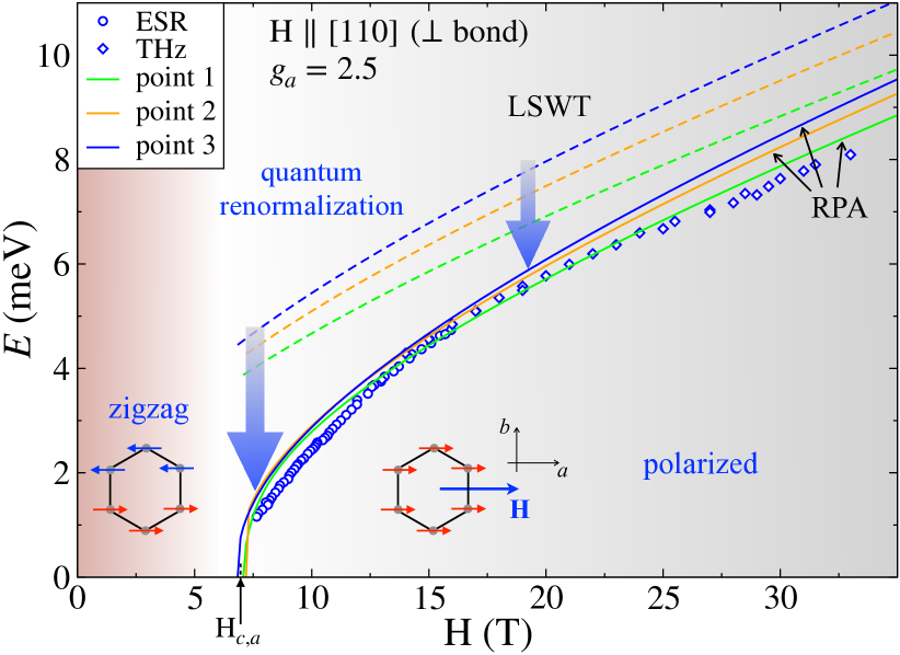
Figure 11: ESR and THz data for the single-magnon energy gap at ${\bf q}\!=\!0$ vs field from Fig. 2 together with the LSWT (dashed lines) and RPA (solid lines) results for the representative points advocated in Sec. II E and Table 1.

With this justification, we now demonstrate the effect of quantum fluctuations on the LSWT results for the single-magnon energy gap at ${\bf q}\!=\!0$ that was anticipated in Fig. 2. The results in Figure 11 are shown for the three representative parameter sets, referred to as Point 1, 2, and 3 in Sec. II E and Table 1. For all three sets, the mean-field RPA already yields a close quantitative description of the ESR/THz data, with the Point 1 set, which belongs to the “realistic” region of the advocated parameter space, giving the best fit of the three.

The variation of the slope of $\varepsilon_{0}(H)$ near the critical point has been attributed to changes of an effective $g$-factor and novel excitations Zvyagin17 . In Ref. kaib19 , this effect has been ascribed to stronger repulsion from the two-magnon continuum in this field regime, which was also supported by the ED calculations. Here we corroborate the latter interpretation using the RPA method, which also shows a significant change of the slope due to enhanced quantum effects near the transition field. In our case, in addition to the field dependence of the LSWT results from Eq. (4), an extra curvature of $\varepsilon_{0}(H)$ is due to the field dependence of the ordered moment $\langle S\rangle$.

	$\langle S\rangle$	$T_{\rm MF}$, K	$T_{N}$, K	$H^{(a)[(b)]}_{c}$, T	$\alpha$,°
Point 1	0.219	16.0	12.3	7.14 [7.88]	28.2
Point 2	0.220	25.4	16.2	7.20 [7.87]	37.2
Point 3	0.225	31.1	21.5	6.94 [7.79]	39.4

Table 2: Zero-field magnetization, Néel temperature, critical fields, and tilt angle for representative parameter sets.

We summarize some of the zero-field properties of the model (1) for the Point 1, 2, and 3 parameter sets in Table 2, where we present spin-wave results for the ordered moment, Néel temperature, critical fields from Eqs. (5) and (6), and tilt angle from Eq. (8) for all three sets.

Our LSWT calculations yield ordered moments that are indicative of strong fluctuations, $\langle S\rangle\!\approx\!0.22$, the value that is in agreement with experimental estimates Coldea15 ; Cao16 and is also similar to the results for the Heisenberg antiferromagnet on the same lattice Weihong91 . While LSWT calculation of the ordered moment $\langle S\rangle$ is standard, the Néel temperature is calculated from a self-consistent condition on the ordered moment $\langle S\rangle\!\rightarrow\!0$ at $T\!\rightarrow\!T_{N}$ within the spin Green’s function formalism using RPA, see Refs. Zhu19 ; Plakida ; Tyablikov and Appendix B for details. One can see a significant lowering of the mean-field results for the ordering temperature, with the latter obtained from $T_{\rm MF}\!=\!-S(S+1)\lambda_{\rm min}(\mathbf{Q})/3k_{B}$, where $\lambda_{\rm min}(\mathbf{Q})$ is the lowest eigenvalue of the Fourier transform of the exchange matrix in (1) at the ordering vector $\mathbf{Q}$ Gingras . The experimental value of $T_{N}$ for $\alpha$-RuCl₃ is known to be sensitive to the stacking of the honeycomb planes Cao16 and can be lower than our values in Table 2, which is likely related to the frustrating 3D interplane couplings Vojta3D .

As was discussed above, the critical fields are not changed by quantum effects within the RPA, as, at the mean-field level, the effect of fluctuations on the field-induced spin polarization cancels the same effect on the gap that is closing at the transition. While this is a mean-field argument, it points to suppressed quantum effects on the critical fields. In Table 2, the critical fields are from Eqs. (5) and (6), and for all three sets they are close to the experimental values for $\alpha$-RuCl₃ NaglerVojta18 . Altogether, the RPA approach provides a good overall description of several aspects of $\alpha$-RuCl₃ phenomenology.

The zero-field ordered moment $\langle S\rangle$ in Table 2 is about the same for all three representative parameter sets, the feature that can be attributed to a significant similarity of the spin-wave spectra in all three cases shown in Fig. 12 for a ${\bf q}$-contour through the Brillouin zone, see Fig. 13 below. The spectra consists of four branches due to the four-sublattice structure of the zigzag state. Since the Point 1, 2 and 3 sets belong to the parameter regions with different bandwidth limits, this provides the main difference between otherwise similar plots.

We also note the pseudo-Goldstone mode at the M point in all three plots that occurs due to an accidental degeneracy. The nature of this degeneracy will be discussed in Sec. IV. The experimental value of the gap at the M point is larger than in our Fig. 12, which is related to the $C_{3}$ symmetry breaking in $\alpha$-RuCl₃ kaib19 ; winter16 . While strongly affecting the gap at the accidental degeneracy points, this lower symmetry is not expected to significantly change other results discussed in this work footnote_C3 .

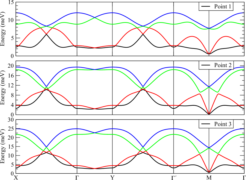
Figure 12: The LSWT magnon spectra for three representative parameter sets, Point 1, 2, and 3 from Sec. II E and Table 1.

III.2 Magnon decays

It was argued in Refs. winter17 ; kopietz20 that strong quantum effects are expected to be generally present in the spectrum of any anisotropic-exchange magnet, except in some narrow regions of its phase diagram where the off-diagonal exchange terms are suppressed. The significant off-diagonal terms necessarily produce strong anharmonic couplings of magnons for any form of the underlying magnetic order. Such couplings, in turn, inevitably lead to a nearly complete wipeout of the higher-energy magnons due to large decay rates into the lower-energy magnon continua RMP13 . As a result, much of the magnon spectrum observed by the inelastic neutron scattering is expected to be comprised of the broad features combined with some well-defined low-energy magnon modes.

Since the preceding consideration unequivocally points to large off-diagonal $\Gamma$ and $\Gamma^{\prime}$ terms in the model (1) of $\alpha$-RuCl₃, there is no question in our mind that the scenario advocated in Refs. winter17 ; kopietz20 is applicable here. Below, we first repeat the general arguments for the inevitability of strong magnon decays, and then apply the approximate analysis of them to a representative set of the model parameters and demonstrate a coexistence of the well-defined low-energy quasiparticles with the broadened excitation continua. We argue that these results are in agreement with the experimental features found in the spectrum of $\alpha$-RuCl₃ nagler16 ; wen17 ; Banerjee17 ; banerjee18 . We underscore, once again, the importance of taking into account magnon decays in interpreting broad features in the spectra of all strongly-anisotropic magnets JeffYbTiO .

III.2.1 General formalism

Within the spin-wave expansion, the reference frame on each site is rotated to a local one with the new $z$ axis pointing along the spin’s quantization axis that is given by the classical energy minimization, $\mathbf{S}_{i}\!=\!\hat{\bf R}_{i}\widetilde{\mathbf{S}}_{i}$. Here, $\widetilde{\mathbf{S}}_{i}$ is the spin vector in the local reference frame at the site $i$ and $\hat{\bf R}_{i}$ is the rotation matrix for that site. For the case of the model (1) of $\alpha$-RuCl₃, this would be a rotation from the cubic axes to the axes of the zigzag order that are tilted out of the basal plane of the honeycomb lattice.

Thus, the spin Hamiltonian (1) can be rewritten as

$$\hat{\cal H}=\sum_{\langle ij\rangle}\widetilde{\mathbf{S}}_{i}^{\rm T}\widetilde{\bm{J}}_{ij}\widetilde{\mathbf{S}}_{j}\,,$$ (10)

where the “rotated” exchange matrix is

$$\widetilde{\bm{J}}_{ij}=\hat{\bf R}_{i}^{\rm T}\hat{\bm{J}}_{ij}\hat{\bf R}_{j}=\left(\begin{array}[]{ccc}\widetilde{J}_{ij}^{xx}&\widetilde{J}_{ij}^{xy}&\widetilde{J}_{ij}^{xz}\\ \widetilde{J}_{ij}^{yx}&\widetilde{J}_{ij}^{yy}&\widetilde{J}_{ij}^{yz}\\ \widetilde{J}_{ij}^{zx}&\widetilde{J}_{ij}^{zy}&\widetilde{J}_{ij}^{zz}\end{array}\right).$$ (14)

For the model (1) one can ignore the third-neighbor Heisenberg exchange terms because they do not contribute to decays for a collinear zigzag order.

The LSWT needs only diagonal and $\widetilde{J}_{ij}^{xy}(\widetilde{J}_{ij}^{yx})$ terms of the matrix $\widetilde{\bm{J}}_{ij}$, while it is its off-diagonal parts that give rise to the three-magnon interaction

$$\mathcal{H}_{\rm od}=\sum_{\langle ij\rangle}\left(\widetilde{J}_{ij}^{xz}\widetilde{S}^{x}_{i}\widetilde{S}^{z}_{j}+\widetilde{J}_{ij}^{yz}\widetilde{S}^{y}_{i}\widetilde{S}^{z}_{j}+\{i\leftrightarrow j\}\right).$$ (15)

The form of the “original” exchange matrix ${\bm{J}}_{ij}$ in (2), in which all terms of the generalized KH model are present, makes it clear that it is only some very restrictive choices of the parameters and ordered states that can render the resultant off-diagonal $\widetilde{J}_{ij}^{xz}$ and $\widetilde{J}_{ij}^{yz}$ terms negligible.

For the zigzag state within the model (2), we obtain explicit expressions of $\widetilde{J}_{ij}^{xz}$ and $\widetilde{J}_{ij}^{yz}$ for each non-equivalent bond in terms of $K$, $\Gamma$, $\Gamma^{\prime}$, and polar and azimuthal angles of the zigzag axes relative to the cubic ones. They are listed in Appendix D. As was discussed in Ref. winter17 , the off-diagonal couplings in Eq. (15) are non-zero except for the case $\Gamma\!=\!\Gamma^{\prime}\!=\!0$, which also makes spins orient along one of the cubic axes. Given that in case of $\alpha$-RuCl₃, $K$ and $\Gamma$ are, in fact, the leading terms of the generalized KH model, it is natural that the off-diagonal couplings $\widetilde{J}_{ij}^{xz}$ and $\widetilde{J}_{ij}^{yz}$ are very significant. Thus, it is imperative to consider their effect in the spin-wave excitations.

The Holstein-Primakoff bosonization of Eq. (15) yields the three-particle interaction

$$\mathcal{H}_{3}=\sum_{\langle ij\rangle}\widetilde{V}_{ij}\left(a^{\dagger}_{i}a^{\dagger}_{j}a^{\phantom{\dagger}}_{j}+\text{H.c}+\{i\rightarrow j\}\right),$$ (16)

where $\widetilde{V}_{ij}\!=\!-\sqrt{S/2}\left(\widetilde{J}_{ij}^{xz}+i\widetilde{J}_{ij}^{yz}\right)$.

While the technical procedure of obtaining fully symmetrized three-magnon interactions from the Holstein-Primakoff form of Eq. (16) typically requires numerical diagonalization of the quadratic LSWT Hamiltonian and is also quite involved otherwise, see Ref. kopietz20 , the resultant form of the decay part of it is general,

$$\hat{\cal H}_{3}\!=\!\frac{1}{2\sqrt{N}}\!\sum_{{\bf k}+{\bf q}=-{\bf p}}\sum_{\eta\nu\mu}\left(\widetilde{V}^{\eta\nu\mu}_{{\bf q}{\bf k};{\bf p}}d^{\dagger}_{\eta{\bf q}}d^{\dagger}_{\nu{\bf k}}d^{\phantom{{\dagger}}}_{\mu-{\bf p}}+{\rm H.c.}\right)\!,\ \ \ \$$ (17)

where $d^{\dagger}(d)$ are magnon operators, indices $\eta$, $\nu$, and $\mu$ numerate magnon branches, and $\widetilde{V}^{\eta\nu\mu}_{{\bf q}{\bf k};{\bf p}}$ is the vertex. With this interaction (17), standard diagrammatic rules allow for a systematic calculation of the quantum corrections to the magnon spectra in the form of self-energies $\Sigma^{\mu}(\mathbf{k},\omega)$.

III.2.2 Approximations

The standard approach, justified within the $1/S$ expansion, is to consider a one-loop correction to the spectrum due to three-magnon interaction (17). Since the most drastic qualitative effect of decays is the finite lifetime, one can ignore the real part of the self-energy of the branch $\mu$ and calculate it in the on-shell approximation, $\Sigma^{\mu}(\mathbf{k},\omega)\!\approx\!-i\Gamma^{\mu}_{{\bf k}}$, where the decay rate of the mode $\mu$ is

$$\Gamma^{\mu}_{{\bf k}}=\frac{\pi}{2N}\sum_{{\bf q},\eta\nu}\big{|}\widetilde{V}^{\eta\nu\mu}_{{\bf q},{\bf k-q};{\bf k}}\big{|}^{2}\delta(\varepsilon_{\mu{\bf k}}-\varepsilon_{\eta{\bf q}}-\varepsilon_{\nu{\bf k-q}}).$$ (18)

Below we will also capitalize on the apparent success of the RPA approach to account for the renormalization of the real part of magnon energies in a simplified fashion.

Generally, the use of Eq. (18) together with the derivation of the vertex in Eq. (17) requires numerical diagonalization of the LSWT Hamiltonian and matrix transformations with potentially prohibitive computational costs. Instead, we use the “constant matrix element” approach that was proposed in Ref. winter17 and was recently validated for the generalized KH model in Ref. kopietz20 , were it was found to provide a good quantitative approximation. We briefly describe its nature below.

The decay rate (18) can be related to a simpler quantity, the on-shell two-magnon density of states (DoS),

$$D_{\mathbf{k}}(\varepsilon_{\mu\bf k})=\frac{\pi}{N}\sum_{\mathbf{q},\nu\eta}\delta\left(\varepsilon_{\mu\mathbf{k}}-\varepsilon_{\nu\mathbf{q}}-\varepsilon_{\eta\mathbf{k-q}}\right),$$ (19)

which quantifies the overlap of the single-magnon excitations of the branch $\mu$ with the two-magnon continuum.

Since we have the full knowledge of the real-space three-magnon vertices in Eq. (16), see Appendix D, we can introduce the overall strength of the coupling

$$\widetilde{V}_{\rm eff}=\frac{1}{12}\sum_{i}\sum_{\langle ij\rangle_{\gamma}}\big{|}\widetilde{V}_{ij}\big{|},$$ (20)

where $i$ sums over four sublattices of the zigzag state and $\gamma\!=\!\{{\rm X,Y,Z}\}$ is numerating the bonds. This definition is consistent with the ones used in Refs. winter17 ; kopietz20 . Then, one can rewrite the three-magnon vertex in Eq. (17) as

$$\widetilde{V}^{\eta\nu\mu}_{{\bf q}{\bf k};{\bf p}}=\widetilde{V}_{\rm eff}\,\widetilde{\Phi}^{\eta\nu\mu}_{{\bf q}{\bf k};{\bf p}},$$ (21)

where the dimensionless vertices $\widetilde{\Phi}$ include all the necessary transformations and symmetrizations.

Within the “constant matrix element” approximation, we substitute the dimensionless $\big{|}\widetilde{\Phi}^{\eta\nu\mu}_{{\bf q},{\bf k-q};{\bf k}}\big{|}^{2}$ in the decay rate (18) by a constant, thus eliminating the numerically costly and analytically cumbersome element of the calculation. As a result, the decay rate (18) is simply proportional to the on-shell two-magnon DoS (19)

$$\Gamma^{\mu}_{\mathbf{k}}\approx\frac{f}{2}\big{|}\widetilde{V}_{\rm eff}\big{|}^{2}D(\varepsilon_{\mu\bf k}),$$ (22)

with an implied relation of the average $f\!=\!\langle\big{|}\widetilde{\Phi}^{\eta\nu\mu}_{{\bf q},{\bf k-q};{\bf k}}\big{|}^{2}\rangle$. This approximation leads to a drastic simplification for the decay rate calculation, as one needs only magnon energies from the harmonic theory and the average real-space three-magnon coupling strength from Eq. (20).

One of the strong justifications of the constant matrix element approximation is the common origin of the Van Hove singularities in the decay rates and the two-magnon DoS. This approximation is also significantly improved by using the self-consistency within the Dyson’s equation, referred to as the iDE approach winter17 ; kopietz20 ; tri09 ; tri_H ; FM_DM ,

$$\Gamma^{\mu}_{{\bf k}}=\frac{f}{2}\big{|}\widetilde{V}_{\rm eff}\big{|}^{2}D^{\mu}_{{\bf k}}(\varepsilon_{\mu\mathbf{k}}+i\Gamma^{\mu}_{{\bf k}}),$$ (23)

where the $\delta$-function with the complex argument is a shorthand for a Lorentzian. Since within the iDE approach there is an effective averaging over various states, it provides further credence to the constant matrix element approximation.

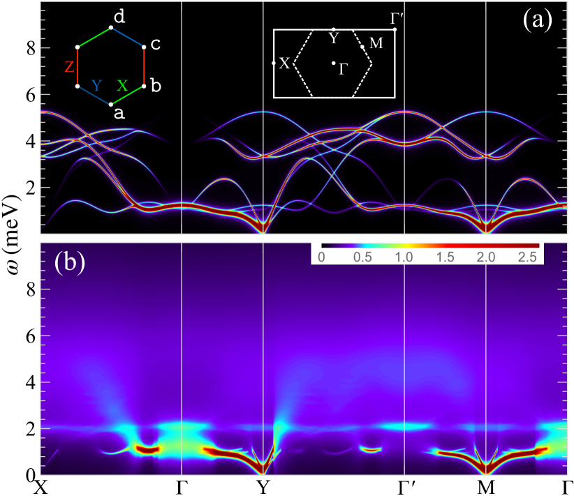
Figure 13: The dynamical structure factor ${\cal S}({\bf q},\omega)$ for the Point 1 parameter set: (a) LSWT results with RPA renormalization, (b) includes magnon lifetime effects and longitudinal contribution, see text.

III.2.3 Results

In Figure 13, we present the results of the calculation of the dynamical structure factor ${\cal S}({\bf q},\omega)$ for the representative parameter set of Point 1 from Sec. II E and Table 1. Fig. 13(a) shows the LSWT results with all energies multiplied by the RPA renormalization factor, $\langle S\rangle/S\approx 0.44$, argued for above, see also Table 2. Since within the LSWT only transverse component of the structure factor contributes, this panel showcases the mean-field renormalization effect of quantum fluctuations on the bare spectrum of Fig. 12. We note that the results in Fig. 13 are averaged over three equivalent domains of the zigzag order, the intensity is cut below the highest maxima in order to emphasize details of the structure factor, and artificial broadening is $\delta\!=\!0.05$ meV.

Fig. 13(b) is our main result. It shows a mix of the contributions of the transverse and longitudinal components of the structure factor, both taking into account magnon lifetime effects on top of the RPA renormalization. Compared to Fig. 13(a), the transverse component includes the decay rates obtained within the iDE approach (23). For the Point 1 parameter set, the calculated overall strength of the three-magnon coupling (20) is $V_{\text{eff}}\!=\!6.1$ meV, which is about half of the bare magnon bandwidth in Fig. 12 for the same set. This value is in accord with the expectations of the significant off-diagonal terms in the exchange matrix laid out above. For the ad hoc parameter $f$ in the calculations of the damping in Eq. (23), the choice was made at $f\!=\!0.1$, which is similar to the ones used in the prior works, see Refs. winter17 ; kopietz20 , where it was based on a comparison with the fully microscopic calculations for the honeycomb-lattice $XXZ$ model in a field hex_H and for the KH-$\Gamma$ model kopietz20 .

As a result of the damping, the upper magnon modes are strongly washed out, with the lower branches damped in some regions of the Brillouin zone and stable in the others. In particular, regions near the $\Gamma$ point are broadened due to decays into the quasi-Goldstone modes, in an accord with the results of Ref. winter17 for a different set of parameters. Overall, the broadening is stronger in the present case because the three-magnon coupling is larger.

An important element to the structure factor in the strongly fluctuating system is the longitudinal component that probes the two-magnon continuum directly. To keep its description on a par with that of the constant matrix element approximation for the decays into such a continuum, we approximate the longitudinal structure factor as directly proportional to the two-magnon density of states with the help of another ad hoc constant parameter, bypassing the need for cumbersome manipulations with the magnon eigenvectors

$$\mathcal{S}^{zz}(\mathbf{q},\omega)=\frac{\pi f_{2}}{N}\sum_{\mathbf{k},\nu\eta}\delta\left(\omega-\widetilde{\varepsilon}_{\nu\mathbf{k}}-\widetilde{\varepsilon}_{\eta\mathbf{q-k}}\right),$$ (24)

where $\widetilde{\varepsilon}_{\nu\mathbf{k}}\!=\!\varepsilon_{\nu\mathbf{k}}+i\Gamma^{\nu}_{\mathbf{k}}$ is the RPA-adjusted magnon energy of the mode $\nu$ together with its damping. Including broadening effects in the magnon lines in Eq. (24) adds another level of self-consistency to our calculation. Here, an improvement over Ref. winter17 is the use of the momentum-dependent $\Gamma^{\nu}_{\mathbf{k}({\bf q-k})}$ instead of the averaged ones, resulting in more pronounced Van Hove singularities in the two-magnon continuum. The choice $f_{2}\!=\!2/15$ is also similar to the prior work winter17 .

In Figure 13(b), the two-magnon longitudinal component provides a strong contribution to the signal at higher energies. Specifically, it contributes to the broad band of intensity between $\approx\!4$ meV and 6 meV, which is in a close accord with the experimental observations of Refs. nagler16 ; banerjee18 that interpreted it as a sign of fractionalization. The two-magnon continuum also extends the observable bandwidth to the values that are consistent with experiments nagler16 ; Banerjee17 ; kaib19 ; Wulferding19 .

The well-defined magnon excitations at low energies are in a qualitative agreement with the neutron scattering results of Refs. wen17 ; banerjee18 . The weak $C_{3}$ symmetry breaking that is present in $\alpha$-RuCl₃ kaib19 ; winter16 is expected to provide a gap at the M points and suppress the decays of the low-energy magnons near the $\Gamma$ point, thus improving the agreement further. The decays of the higher-energy magnons and the broad band of intensity are expected to be insensitive to such a symmetry breaking.

Altogether, our results strongly substantiate the expectations outlined in the beginning of this Section. The results of our calculations for a representative parameter set from the realistic parameter region yield the spectrum that is comprised of the broad excitation continua coexisting with the well-defined low-energy magnon modes. In accord with the scenario advocated in Refs. winter17 ; kopietz20 , it highlights the significance of the phenomenon of magnon decays and outlines the challenges of interpreting broad features in the spectra of strongly-anisotropic magnets.

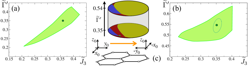
Figure 14: (a) The $\widetilde{\Gamma}^{\prime}$–$\widetilde{J}_{3}$ projection of the “realistic” ($W_{0}\!<\!15$ meV) parameter region from Sec. II, see also Figs. 6–9; $\widetilde{\Gamma}^{\prime}$ and $\widetilde{J}_{3}$ are $\Gamma^{\prime}$ and $J_{3}$ in units of $\sqrt{J^{2}+K^{2}+\Gamma^{2}}$. (b) Same projection after duality transformation of Eq. (37). (c), bottom: a sketch of the $\pi$-rotation in the honeycomb plane about crystallographic $z_{0}$ axis. (c), top: a schematic illustration of the transition between the two planes of the $J$–$K$–$\Gamma$ phase diagrams in Fig. 15 along the $\widetilde{\Gamma}^{\prime}$-axis of an extended cylindrical 3D phase diagram as a result of the duality transformation.

IV Dual models and other forms

In this Section we provide further insights into the relevant section of the phase diagram of the generalized KH model that is pertinent to $\alpha$-RuCl₃ parameter space, analyze it with the help of the duality transformations, and discuss possible simplified versions of the effective model that should contain essential physics of this material.

IV.1 Dualities

The generalized KH model (2) is known to map onto itself under various transformations Kimchi14 ; CJK13 ; ChKh15 , contributing to the aura of sophistication surrounding this model. While some of such transformations are rather non-trivial, others occur under benign symmetry operations, with the latter made not obvious by the parametrization of the exchange matrix (2) in the cubic axes.

One of such artifacts of the cubic axes representation is the self-duality under the $\pi$-rotation of the honeycomb plane about crystallographic $z_{0}$ axis ([111] direction in the cubic axes), see Fig. 1 and Fig. 14. While for the model in crystallographic axes (see below) this innocent symmetry operation leads to an inconsequential sign change in one of the terms (${\sf J_{z\pm}}$), it requires rewriting of the generalized KH model (2) within the rotated set of the cubic axes ChKh15 , transforming its parameters as

$$\left(\begin{array}[]{c}J\\ K\\ \Gamma\\ \Gamma^{\prime}\end{array}\right)_{\rm dual}=\left(\begin{array}[]{cccc}1&+\frac{4}{9}&-\frac{4}{9}&+\frac{4}{9}\\ 0&-\frac{1}{3}&+\frac{4}{3}&-\frac{4}{3}\\ 0&+\frac{4}{9}&+\frac{5}{9}&+\frac{4}{9}\\ 0&-\frac{2}{9}&+\frac{2}{9}&+\frac{7}{9}\end{array}\right)\left(\begin{array}[]{c}J\\ K\\ \Gamma\\ \Gamma^{\prime}\end{array}\right).$$ (37)

It is important to note that models with the dual and original parameters lead to identical physical outcomes.

Because of that, the utility of such duality transformations is that they can reveal the origin of some properties of the generalized KH model that are hidden in the original language. For instance, for the same model on the triangular lattice, the so-called Klein duality has allowed to relate an enigmatic quasi-Goldstone mode in the stripe phase to an accidental degeneracy in the Klein-dual ferromagnetic phase Zhu19 . In the spectrum of $\alpha$-RuCl₃, quasi-Goldstone modes are ubiquitously present at the M points that are complementary to the ordering vector of the zigzag phase wen17 ; banerjee18 , suggesting a proximity to an accidental degeneracy. This is also true throughout the parameter space advocated in Sec. II, as is highlighted in Fig. 12 for representative parameter sets.

Here, we use duality transformations to shed light on the relevant phase diagram and properties of $\alpha$-RuCl₃. In Fig. 14(a), we show $\widetilde{\Gamma}^{\prime}$–$\widetilde{J}_{3}$ projection of the “realistic” parameter region, see Sec. II, where $\widetilde{\Gamma}^{\prime}$ and $\widetilde{J}_{3}$ are $\Gamma^{\prime}$ and $J_{3}$ normalized by $\sqrt{J^{2}+K^{2}+\Gamma^{2}}$, which is used as an energy scale, reducing the parameter space dimensions to 4D. Fig. 14(b) shows the same projection after duality transformation of Eq. (37).

To make possible an exploration of the wider phase diagram, we choose a representative point from the “original” projection in Fig. 14(a), $\{\widetilde{\Gamma}^{\prime},\widetilde{J}_{3}\}\!=\!\{0.35,0.36\}$. Since this fixes two parameters of the 4D parameter space, we can investigate the remaining $J$–$K$–$\Gamma$ phase diagram by the Luttinger-Tisza method LT , see Fig. 15(a) for the polar representation of it, in which $\Gamma$ is the radial and $J$ and $K$ are the polar variables.

The entire phase space is exhausted by the aniferromagnetic (AFM), zigzag (ZZ), and the incommensurate (IC) states. The parameter space associated with the “realistic” parameter choices occupies a small region of the zigzag phase bordering incommensurate phase, as is discussed in Sec. II D, see also Appendix C. The zigzag-to-incommensurate phase transition is of the first order by both LT and LSWT analysis. The IC phase evolves continuously from a ferromagnetic state in a broader $\widetilde{\Gamma}^{\prime}$–$\widetilde{J}_{3}$ parameter space and is similar in nature to the helical phase within the phase diagram of the $J_{1}$–$J_{2}$–$J_{3}$ model on the same lattice italians79 .

It is the dual $\pi$-rotated version of this phase diagram that is of interest. A minor subtlety occurs because the transformation of Eq. (37) concerns all four parameters of the exchange matrix, so that the transformation of the single point in Fig. 14(a) results in an area in the dual $\widetilde{\Gamma}^{\prime}$–$\widetilde{J}_{3}$ projection in Fig. 14(b), which is highlighted by the ellipse. To make a comparison meaningful and given a small size of the dual region of interest, we also pick a representative point in the dual region of parameters, $\{\widetilde{\Gamma}^{\prime},\widetilde{J}_{3}\}\!=\!\{0.54,0.35\}$, see Fig. 14(b). We also note that since the duality transformation (37) involves four parameters, one can see it as a transition between the planes of a 3D cylindrical phase diagram along the $\widetilde{\Gamma}^{\prime}$-axis, as is schematically illustrated in Fig. 14(c).

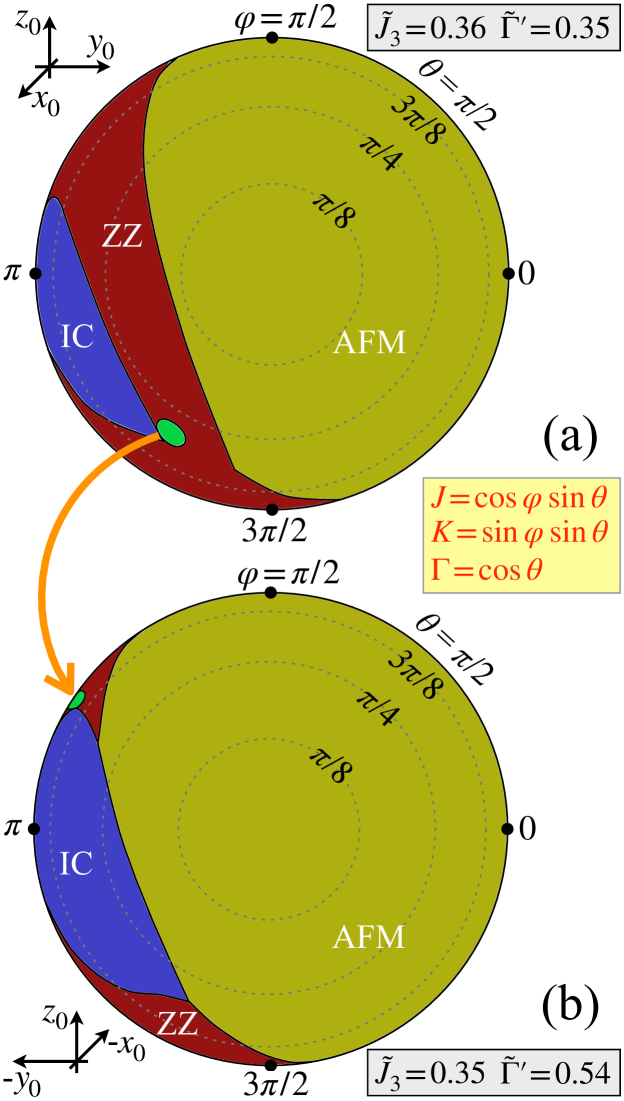
Figure 15: (a) The $J$–$K$–$\Gamma$ phase diagram for $\{\widetilde{\Gamma}^{\prime},\widetilde{J}_{3}\}\!=\!\{0.35,0.36\}$, and (b) for $\{\widetilde{\Gamma}^{\prime},\widetilde{J}_{3}\}\!=\!\{0.54,0.35\}$, see text.

The dual $J$–$K$–$\Gamma$ phase diagram for this choice of $\widetilde{\Gamma}^{\prime}$ and $\widetilde{J}_{3}$ is shown in Fig. 15(b). The most important observation is that the duality-transformed “realistic” parameter region of the generalized KH model corresponds to the vanishing values of the $\Gamma$-term. This is also corroborated by the dual transformation (37) of the Point 1, 2, and 3 representative parameter sets of the model from Sec. II E, given by the following dual $(K,\Gamma,\Gamma^{\prime},J,J_{3})$ coordinates (in meV)

	$(K,$	$\Gamma,$	$\Gamma^{\prime},$	$J,$	$J_{3})\$
dual Point 1:	(3.71,	1.24,	3.92,	-5.40,	2.42)
dual Point 2:	(6.67,	-0.62,	5.81,	-9.82,	3.26)
dual Point 3:	(8.72,	-1.72,	7.20,	-12.32,	3.66).

In all three cases, as well as in Fig. 15(b), the allowed parameters correspond to $\Gamma\!\approx\!0$, dominant ferromagnetic $J\!<\!0$, followed by substantial antiferromagnetic Kitaev and $\Gamma^{\prime}$ terms, $K\!\approx\!\Gamma^{\prime}\!>\!0$. The dual zigzag region is also bordered by the incommensurate phase because the global $\pi$-rotation does not affect the ground state. We emphasize once more that the resultant physical properties of the original and dual models are identical.

The duality of the original model to the one with negligible $\Gamma$ sheds new light onto the nature of the persistent pseudo-Goldstone modes in $\alpha$-RuCl₃ wen17 ; banerjee18 . The pure Kitaev-Heisenberg model with $\Gamma\!=\!\Gamma^{\prime}\!=\!0$ is well-known to have a classical accidental degeneracy leading to a gapless mode Kimchi14 ; CJK13 . Such a degeneracy is generally lifted by $\Gamma\!\neq\!0$. It is less known that the non-zero $\Gamma^{\prime}$ term can leave this degeneracy intact RauGp . The logic of this behavior is exposed by the four-sublattice Klein duality transformation that converts zigzag to antiferromagnetic state Kimchi14 ; CJK13 . While this transformation maps pure Kitaev-Heisenberg model onto itself, the off-diagonal $\Gamma^{\prime}$ term morphs into antisymmetric, Dzyaloshinskii-Moriya-like interaction $\breve{\Gamma}^{\prime}$. The latter does not affect collinear ground state on a classical level, leaving the accidental degeneracy intact and preserving pseudo-Goldstone modes. This effect is similar to the one discussed for the same model on the triangular lattice Zhu19 .

IV.2 Simpler models

The other reason why the negligible-$\Gamma$ form of the generalized KH model is important, is because it results in an effective description of $\alpha$-RuCl₃ by fewer parameters. The relevant $K$–$J$–$\Gamma^{\prime}$–$J_{3}$ model has a lower dimensionality of its parameter space and is, thus, more amendable to a detailed exploration.

A potentially more drastic simplification can be achieved by rewriting the model (1) in the “spin-ice” language that uses crystallographic axes Ross11 ; RauGp ; ChKh15 ; RauYb ; Tsirlin_Review ; Zhu19 , where $x_{0}$ and $y_{0}$ correspond to the $a$ and $b$ directions in the plane of the honeycomb lattice, see Fig. 1. This leads to the $XXZ$–${\sf J_{\pm\pm}}$–${\sf J_{z\pm}}$ form of the Hamiltonian (1)

$${\cal H}_{1}=\sum_{\langle ij\rangle}\Big{[}{\sf J_{1}}\Big{(}S^{x_{0}}_{i}S^{x_{0}}_{j}+S^{y_{0}}_{i}S^{y_{0}}_{j}+\Delta S^{z_{0}}_{i}S^{z_{0}}_{j}\Big{)}$$ (38)

$$\!-\!2{\sf J_{\pm\pm}}\Big{(}\Big{(}S^{x_{0}}_{i}S^{x_{0}}_{j}\!-\!S^{y_{0}}_{i}S^{y_{0}}_{j}\Big{)}\tilde{c}_{\alpha}\!-\!\Big{(}S^{x_{0}}_{i}S^{y_{0}}_{j}\!+\!S^{y_{0}}_{i}S^{x_{0}}_{j}\Big{)}\tilde{s}_{\alpha}\Big{)}$$

$$\!-\!{\sf J_{z\pm}}\Big{(}\Big{(}S^{x_{0}}_{i}S^{z_{0}}_{j}\!+\!S^{z_{0}}_{i}S^{x_{0}}_{j}\Big{)}\tilde{c}_{\alpha}\!+\!\Big{(}S^{y_{0}}_{i}S^{z_{0}}_{j}\!+\!S^{z_{0}}_{i}S^{y_{0}}_{j}\Big{)}\tilde{s}_{\alpha}\Big{)}\Big{]},$$

where abbreviations are $\tilde{c}_{\alpha}\!=\!\cos\tilde{\varphi}_{\alpha}$ and $\tilde{s}_{\alpha}\!=\!\sin\tilde{\varphi}_{\alpha}$, bond-dependent phases $\tilde{\varphi}_{\alpha}\!=\!\{0,2\pi/3,-2\pi/3\}$ correspond to the $\{{\rm Z,X,Y}\}$ bonds in Fig. 1, respectively, and the isotropic third-neighbor ${\cal H}_{3}$ is unchanged.

The relation of the parameters of the model (38) to the parameters of the model (2) is given in Appendix A. Rewriting the Point 1, 2, and 3 representative parameter sets from Sec. II E in these new variables yields

	$({\sf J_{1}},$	$\Delta,$	${\sf J_{\pm\pm}},$	${\sf J_{z\pm}},$	$J_{3})\$
“ice” Point 1:	(-7.20,	-0.26,	0.3,	-3.0,	2.42)
“ice” Point 2:	(-11.3,	0.02,	1.0,	-6.2,	3.26)
“ice” Point 3:	(-13.6,	0.07,	1.5,	-8.3,	3.66),

all in meV except for the dimensionless $XXZ$ anisotropy parameter $\Delta$.

It transpires that for all three representative sets, the easy-plane anisotropy $\Delta$ is small and one of the bond-dependent terms ${\sf J_{\pm\pm}}$ is much smaller than the other interactions. We can verify that the same is true across the advocated realistic parameter ranges for $\alpha$-RuCl₃: the model in the language of Eq. (38) consistently has these two terms nearly negligible. Some of the parameter sets suggested in the prior works based on $\alpha$-RuCl₃ phenomenology also follow the same trend winter17 . Of the remaining terms, the leading is the ferromagnetic $XY$ exchange ${\sf J_{1}}$ with the sizable ${\sf J_{z\pm}}\!\approx\!|{\sf J_{1}}|/2$ and $J_{3}$.

It follows from this analysis that the ${\sf J_{1}}$–${\sf J_{z\pm}}$–$J_{3}$ model, written in crystallographic axes of the honeycomb lattice and operating in a much more accessible 3D parameter space, should be able to offer a much simpler and much more natural way of describing $\alpha$-RuCl₃ that can give a refreshing perspective on its physics.

It also appears that the relevant physics of $\alpha$-RuCl₃ is not related to a model with a dominating Kitaev term, but is that of the easy-plane ferromagnet with antiferromagnetic third-neighbor coupling and strong off-diagonal exchange ${\sf J_{z\pm}}$. Naturally, it is the latter term that is responsible for the out-of-plane tilting of the ordered moment, substantial fluctuations in the ground state, and significantly damped magnon excitations.

From this study, one is also led to believe that it is not a proximity to a Kitaev spin-liquid phase, but a proximity to an incommensurate phase, which is continuously connected to a ferromagnetic one, that is significantly more pertinent to the phase diagram of $\alpha$-RuCl₃. These and other features of this material and relevant models deserve further investigation.

V Summary

We conclude by summarizing our results.

We have demonstrated that empirical constraints lead to significant restrictions and rather drastic revisions of the physically reasonable parameter space for the effective microscopic spin model of $\alpha$-RuCl₃. Specifically, the ESR and THz data in the field-induced paramagnetic regime, combined with the analysis of the in-plane critical fields, out-of-plane tilt angle, bandwidth of the magnetic signal, and the zigzag nature of the ground state, produce convincing bounds on the parameters of this model.

In broad strokes, for the key parameters of the generalized KH model, these constraints necessitate a significant positive $\Gamma^{\prime}\!\approx\!\Gamma/2$ not anticipated previously and a close relation $J\!+\!3J_{3}\!\approx\!\Gamma$. The leading Kitaev term $K\!<\!0$ is also constrained and is not overly dominating, with the ratio $|K|/\Gamma\!\approx\!1.0-3.0$, and $J\!<\!0$ and $J_{3}\!>\!0$ terms varying within the range of $|J|/\Gamma\!\approx\!J_{3}/\Gamma\!\approx\!0.5-0.75$. In the absolute units, the bounds on $\Gamma$ are $\approx\!4$ meV$-$6 meV, setting the scale for the rest of the model.

We have also demonstrated that our proposed parameter sets provide an excellent account of a variety of other phenomenologies of $\alpha$-RuCl₃, allowing to consolidate previous attempts of their description. Our parameters can be reconciled with the typically smaller parameters discussed in the prior works by suggesting their renormalization due to quantum fluctuations. We have shown that the latter effect can be successfully approximated with the help of a self-consistent mean-field RPA approach.

We have argued, in accord with the previous studies, that the off-diagonal terms that necessarily produce strong anharmonic couplings of magnons are expected to be significant throughout the phase diagram of an anisotropic-exchange magnet and for any form of the underlying magnetic order. These couplings, in turn, inevitably lead to large decay rates of the higher-energy into the lower-energy magnons, resulting in a coexistence of the broad continua with the well-defined low-energy modes in the inelastic neutron scattering spectrum. The proposed parameter space of $\alpha$-RuCl₃ is no exception to this scenario, with our calculations of the dynamical structure factor for a representative parameter set strongly substantiating it in a close agreement with experiments. This result highlights the challenges of interpreting broad features in the spectra of strongly-anisotropic magnets and the significance of the phenomenon of magnon decays in this context.

We have also provided an important insight into the nature of the pseudo-Goldstone modes that occur away from the ordering vector of the zigzag phase of $\alpha$-RuCl₃. Using duality transformations of the generalized KH model within the advocated parameter range, we have related these modes to an accidental near-degeneracy in a duality-related $\Gamma$-less model, in which the degeneracy of the pure Kitaev-Heisenberg type is not lifted by the $\Gamma^{\prime}$ term. As a by-product, this effort has suggested a fully equivalent simpler model description of $\alpha$-RuCl₃ within the same KH model, but with the leading term $J\!<\!0$, subleading positive $K\!\approx\!\Gamma^{\prime}$, finite $J_{3}$, and negligible $\Gamma$.

A different and substantially more radical simplification advocated in this work is the rewriting of the generalized KH model in the natural crystallographic axes of the honeycomb lattice. We have verified that for the advocated realistic parameter ranges of $\alpha$-RuCl₃, the model in this language has only three substantial terms: the leading ferromagnetic easy-plane ${\sf J_{1}}$, antiferromagnetic $J_{3}$, and a sizable off-diagonal term ${\sf J_{z\pm}}$. The latter term favors the observed out-of-plane tilting of spins in the zigzag phase and its role in strong quantum effects and magnon interactions deserves further investigation.

Thus, one of the key result of the rethinking endeavor undertaken in this work is that the relevant physics of $\alpha$-RuCl₃ is not related to a model with a dominating Kitaev term, but must be understood and revisited as that of the ${\sf J_{1}}$–$J_{3}$ FM-AFM model with the dominant easy-plane ${\sf J_{1}}$ and a strong off-diagonal exchange ${\sf J_{z\pm}}/|{\sf J_{1}}|\!\approx\!0.5$.

Altogether, the provided consideration of the $\alpha$-RuCl₃ phenomenologies and its effective model unequivocally suggests that the physics of this material is not affiliated with a proximate spin-liquid state. The only proximity in the phase diagram that is present in this case and may be worth exploring is that to an incommensurate phase, which is continuously connected to a ferromagnetic one. For the much-discussed spectral properties of $\alpha$-RuCl₃, the conclusion of this work also unambiguously points toward the physics of the strongly interacting and mutually decaying magnons, not to that of the fractionalized excitations.

Appendix A LSWT details

The “spin-ice” form of the Hamiltonian (2) in the crystallographic $\{x_{0},y_{0},z_{0}\}$ axes of the honeycomb plane is given by Eq. (38). Its parameters are related to that of the generalized KH model in the cubic axes (2) via

$${\sf J_{1}} =J+\frac{1}{3}\big{(}K-\Gamma-2\Gamma^{\prime}\big{)},$$

$$\Delta{\sf J_{1}} =J+\frac{1}{3}\big{(}K+2\Gamma+4\Gamma^{\prime}\big{)},$$

$$2{\sf J_{\pm\pm}} =-\frac{1}{3}\big{(}K+2\Gamma-2\Gamma^{\prime}\big{)},$$ (39)

$$\sqrt{2}{\sf J_{z\pm}} =\frac{2}{3}\big{(}K-\Gamma+\Gamma^{\prime}\big{)}.$$

The rotation to the local reference frame of spins for the field-induced polarized paramagnetic state with the subsequent Holstein-Primakoff and Fourier transformations in (38) yield the LSWT Hamiltonian

$$\mathcal{H}=\frac{1}{2}\sum_{\mathbf{k}}\mathbf{x}_{\mathbf{k}}^{\dagger}\mathbf{H_{k}}\mathbf{x}_{\mathbf{k}}^{\phantom{\dagger}},$$ (40)

where $\mathbf{x}_{\mathbf{k}}\!=\!\big{(}a^{\phantom{\dagger}}_{\mathbf{k}},b^{\phantom{\dagger}}_{\mathbf{k}},a^{\dagger}_{\mathbf{-k}},b^{\dagger}_{\mathbf{-k}}\big{)}$, and $a_{\mathbf{k}}$ and $b_{\mathbf{k}}$ are bosonic magnon operators on two sublattices of the honeycomb lattice. The form of the Hamiltonian in the polarized phase for the principal in-plane field directions is

$$\mathbf{H}=\left(\begin{array}[]{cccc}A_{\mathbf{k}}&B_{\mathbf{k}}&0&C_{\mathbf{k}}\\ B^{*}_{\mathbf{k}}&A_{\mathbf{k}}&C_{\mathbf{-k}}&0\\ 0&C^{*}_{\mathbf{-k}}&A_{\mathbf{k}}&B_{\mathbf{k}}\\ C^{*}_{\mathbf{k}}&0&B^{*}_{\mathbf{k}}&A_{\mathbf{k}}\end{array}\right),$$ (45)

where for $H\!\parallel\!a$

$$A_{\mathbf{k}} =g\mu_{B}H-3S\big{(}{\sf J_{1}}+J_{3}\big{)},$$

$$B_{\mathbf{k}} =\frac{3S}{2}\left[{\sf J_{1}}\big{(}1+\Delta\big{)}\gamma_{\mathbf{k}}+2J_{3}\gamma^{(3)}_{\mathbf{k}}+2{\sf J_{\pm\pm}}\gamma^{\prime}_{\mathbf{k}}\right],$$ (46)

$$C_{\mathbf{k}} =-\frac{3S}{2}\left[{\sf J_{1}}\big{(}1-\Delta\big{)}\gamma_{\mathbf{k}}+2{\sf J_{\pm\pm}}\gamma^{\prime}_{\mathbf{k}}-2i{\sf J_{z\pm}}\gamma^{\prime\prime}_{\mathbf{k}}\right],$$

and for $H\!\parallel\!b$

$$A_{\mathbf{k}} =g\mu_{B}H-3S\big{(}{\sf J_{1}}+J_{3}\big{)},$$

$$B_{\mathbf{k}} =\frac{3S}{2}\big{[}{\sf J_{1}}\big{(}1+\Delta\big{)}\gamma_{\mathbf{k}}+2J_{3}\gamma^{(3)}_{\mathbf{k}}-2{\sf J_{\pm\pm}}\gamma^{\prime}_{\mathbf{k}}\big{]},$$ (47)

$$C_{\mathbf{k}} =\frac{3S}{2}\big{[}{\sf J_{1}}\big{(}1-\Delta\big{)}\gamma_{\mathbf{k}}-2{\sf J_{\pm\pm}}\gamma^{\prime}_{\mathbf{k}}+2i{\sf J_{z\pm}}\gamma^{\prime}_{\mathbf{k}}\big{]},$$

where the hopping functions are given by

$$\gamma_{\mathbf{k}} =\frac{1}{3}\sum_{\alpha=1}^{3}e^{i\mathbf{k}{\bm{\delta}}_{\alpha}},\ \ \ \gamma^{(3)}_{\mathbf{k}}=\frac{1}{3}\sum_{\alpha=1}^{3}e^{i\mathbf{k}{\bm{\delta}}^{(3)}_{\alpha}},$$ (48)

$$\gamma^{\prime}_{\mathbf{k}} =\frac{1}{3}\sum_{\alpha=1}^{3}\cos\tilde{\varphi}_{\alpha}e^{i\mathbf{k}{\bm{\delta}}_{\alpha}},\ \ \ \gamma^{\prime\prime}_{\mathbf{k}}=\frac{1}{3}\sum_{\alpha=1}^{3}\sin\tilde{\varphi}_{\alpha}e^{i\mathbf{k}{\bm{\delta}}_{\alpha}},$$ (49)

and ${\bm{\delta}}_{\alpha}$ are the vectors connecting nearest-neighbor sites along the ${\{\rm Z,X,Y\}}$ bonds, respectively, see Fig. 1.

The LSWT spectrum is given by the standard procedure for a bosonic Hamiltonian Colpa , which requires diagonalization of $\mathbf{g}\mathbf{H_{k}}$, where $\mathbf{g}$ is a diagonal matrix $\{1,1,-1,-1\}$. For $\mathbf{H_{k}}$ in Eq. (45) this diagonalization can be done analytically and the eigenvalues are given by the solutions of the biquadratic equation

$$\lambda^{4}-2k\lambda^{2}+c=0,$$ (50)

where

$$k =A_{\mathbf{k}}^{2}+\big{|}B_{\mathbf{k}}\big{|}^{2}-\frac{\big{|}C_{\mathbf{k}}\big{|}^{2}+\big{|}C_{\mathbf{-k}}\big{|}^{2}}{2},$$ (51)

$$c =\big{(}A_{\mathbf{k}}^{2}-\big{|}B_{\mathbf{k}}\big{|}^{2}\big{)}^{2}-A_{\mathbf{k}}^{2}\big{(}\big{|}C_{\mathbf{k}}\big{|}^{2}+\big{|}C_{\mathbf{-k}}\big{|}^{2}\big{)}$$

$$+\big{|}C_{\mathbf{k}}\big{|}^{2}\big{|}C_{\mathbf{-k}}\big{|}^{2}-B_{\mathbf{k}}^{2}C_{\mathbf{-k}}C^{*}_{\mathbf{k}}-(B^{*}_{\mathbf{k}})^{2}C^{*}_{\mathbf{-k}}C_{\mathbf{k}}.$$

These expressions simplify for the high-symmetry $\mathbf{k}$ points. First, the magnon spectrum at the $\Gamma$ point, $\mathbf{k}\!=\!0$, for both field directions is

$$\varepsilon_{1,2}=\sqrt{\big{(}A_{\mathbf{k}}\pm B_{\mathbf{k}}\big{)}^{2}-\big{|}C_{\mathbf{k}}\big{|}^{2}}.$$ (52)

In particular, the lowest mode as a function of magnetic field is given by

$$\varepsilon_{1,\mathbf{k}=0} =\sqrt{g\mu_{B}H\big{(}g\mu_{B}H-3{\sf J_{1}}S(1-\Delta)\big{)}}.$$ (53)

Translation to the generalized KH interactions via (39) yields Eq. (4) in Sec. II.1.

For the field $H\!\parallel\!a$, the important high-symmetry points are the $M$ points, $\mathbf{k}_{M(M^{\prime})}\!=\!\big{(}\pi/\sqrt{3},\pm\pi\big{)}$. The matrix elements in Eq. (46) for these points, with the help of the transformation $b_{\mathbf{k}}\!\rightarrow\!b_{\mathbf{k}}e^{\pm i\pi/3}$, simplify to

$$A_{\mathbf{k}} =g\mu_{B}H-3S\big{(}{\sf J_{1}}+J_{3}\big{)},$$

$$B_{\mathbf{k}} =\frac{S}{2}\big{[}{\sf J_{1}}\big{(}1+\Delta\big{)}-6J_{3}+2{\sf J_{\pm\pm}}\big{]},$$ (54)

$$C_{\mathbf{k}} =-\frac{S}{2}\big{[}{\sf J_{1}}\big{(}1-\Delta\big{)}+2{\sf J_{\pm\pm}}+2\sqrt{3}i{\sf J_{z\pm}}\big{]},$$

and the magnon energies are given by the same Eq. (52). From Eqs. (52) and (54), one obtains a transition field from the polarized to zigzag phase by finding $H_{c}$ that corresponds to closing of the gap at the $M$ points, $\varepsilon_{1,\mathbf{k}}\!=\!0$, resulting in Eq. (5).

For the field in the $b$-direction, the gap closes at the $Y$ point and the matrix elements for $\mathbf{k}_{Y}\!=\!\big{(}2\pi/\sqrt{3},0\big{)}$ in Eq. (47) are given by

$$A_{\mathbf{k}} =g\mu_{B}H-3S({\sf J_{1}}+J_{3}),$$

$$B_{\mathbf{k}} =\frac{S}{2}\big{[}{\sf J_{1}}\big{(}1+\Delta\big{)}-6J_{3}+4{\sf J_{\pm\pm}}\big{]},$$ (55)

$$C_{\mathbf{k}} =\frac{S}{2}\big{[}{\sf J_{1}}\big{(}1-\Delta\big{)}+4{\sf J_{\pm\pm}}-4i{\sf J_{z\pm}}\big{]}.$$

The solution for the gap closure gives the critical field in the $b$-direction, Eq. (6).

Appendix B Self-consistent calculation of the Néel temperature

The spin Green’s function in the self-consistent RPA approximation is given by Tyablikov ; Plakida ; Zhu19

$$\langle S^{-}_{\mathbf{k}}S^{+}_{\mathbf{-k}}\rangle_{\omega}=2\langle S\rangle\sum_{\mu}\left(\frac{u_{\mu\mathbf{k}}^{2}}{\omega-\widetilde{\varepsilon}_{\mu\mathbf{k}}}-\frac{v_{\mu\mathbf{k}}^{2}}{\omega+\widetilde{\varepsilon}_{\mu\mathbf{k}}}\right),$$ (56)

where $u_{\mu\mathbf{k}}$ and $v_{\mu\mathbf{k}}$ are parameters of the generalized Bogolyubov transformation that diagonalizes the spin-wave bosonic Hamiltonian, $\mu$ numerates bosonic branches in the zigzag phase, and $\widetilde{\varepsilon}_{\mu\mathbf{k}}\!=\!2\langle S\rangle\varepsilon_{\mu\mathbf{k}}$, see Eq. (9).

A self-consistent condition on the ordered moment is obtained from $S^{z}_{i}=\frac{1}{2}-S^{-}_{i}S^{+}_{i}$ using spectral representation in Eq. (56), resulting in

$$\langle S\rangle=\frac{1}{2}-\frac{2\langle S\rangle}{N}\sum_{\mu,\mathbf{k}}\Big{(}u_{\mu\mathbf{k}}^{2}n\left(\widetilde{\varepsilon}_{\mu\mathbf{k}}\right)-v_{\mu\mathbf{k}}^{2}n\left(-\widetilde{\varepsilon}_{\mu\mathbf{k}}\right)\Big{)}.\ \ \ \ \ \$$ (57)

where $n(\omega)$ is the Bose distribution function.

At $T\!\rightarrow\!T_{N}$, the ordered moment $\langle S\rangle\!\rightarrow\!0$ and (57) yields the ordering temperature

$$\frac{1}{T_{N}}=\frac{2}{N}\sum_{\mu,\mathbf{k}}\frac{u_{\mu\mathbf{k}}^{2}+v_{\mu\mathbf{k}}^{2}}{\varepsilon_{\mu\mathbf{k}}}.$$ (58)

Note that the outlined approach is valid only for $S\!=\!1/2$, with the formalism becoming more complicated for larger spins Tyablikov .

Appendix C $J$–$J_{3}$ phase diagram for fixed $\{K,\Gamma,\Gamma^{\prime}\}$

A useful insight can be provided by using a “strict” form of the proposed constraints and examining the remaining low(er)-dimensional parameter space for its phase diagram. This approach can also help to alleviate a concern that the 2D projections from a higher-dimensional parameter space with the dimensions higher than 3D can give a false perception of the phase diagram. This is because such 2D projections simply demonstrate the largest possible extent of the allowed parameters, which can be significantly different for different lower-dimensional “cuts” of the higher-dimensional object.

Here, we use our constraints on ESR/THz gap, $\Delta H_{c}$, and tilt-angle $\alpha$, by strictly fixing them to the values that are close to, or motivated by, the experiments. Thus, we fix $\Gamma_{\rm tot}\!=\!9$ meV, $\Delta H_{c}\!=\!1$ T, and $\alpha\!=\!35^{\degree}$ according to the discussions in Secs. II A–D. Since, quasiclassically, these quantities depend only on $K$, $\Gamma$, and $\Gamma^{\prime}$ combinations, this specific choice of constraints yields the following set of $\{K,\Gamma,\Gamma^{\prime}\}\!=\!\{-7.567,4.276,2.362\}$ meV. We will refer to it as to the “Point 0 set” below.

Figure 16: The $J$–$J_{3}$ phase diagram for $J\!<\!0$ and $J_{3}\!>\!0$ at fixed $\{K,\Gamma,\Gamma^{\prime}\}\!=\!\{-7.567,4.276,2.362\}$ meV, see text. The highlighted regions are the zigzag (ZZ), ferromagnetic (FM), and incommensurate phases (IC).

Of the 5D parameter space, only $J$ and $J_{3}$ parameters remain. This allows us to explore the 2D $J$–$J_{3}$ phase diagram for the relevant ranges of $J\!<\!0$ and $J_{3}\!>\!0$, presented in Fig. 16. The highlighted regions correspond to the zigzag (ZZ), ferromagnetic (FM), and incommensurate (IC) phases. Our last constraint that can be made rigid is to fix $H_{c}^{(a)}\!=\!H_{c}^{(a)}(K,\Gamma,\Gamma^{\prime},J_{03})$ to its experimental value of $H_{c,{\rm exp}}^{(a)}\!=\!7$T, see Sec. II C. This binds $J_{03}\!=\!J+3J_{3}$ from Eq. (7), yielding $J_{03}\!=\!4.768$ meV and restricting $J$ and $J_{3}$ to the straight line shown in Fig. 16.

Altogether, this consideration illustrates that the values of $|J|$ and $J_{3}$ that are needed to stabilize the zigzag phase are larger than is typically assumed, see Table 1. Another important observation is that the empirically-constrained parameter sets put $\alpha$-RuCl₃ in the proximity of an incommensurate phase. As is discussed in Sec. IV, this phase is reminiscent of that in the phase diagram of the $J_{1}$–$J_{2}$–$J_{3}$ model on the honeycomb lattice and is continuously connected to a ferromagnetic state.

Appendix D Off-diagonal terms in Eq. (15)

There are five distinct bonds regarding the values of $\widetilde{J}_{ij}^{xz}$, $\widetilde{J}_{ij}^{yz}$ or their combinations. Keeping explicit the angles $\varphi$ and $\theta$, which are defined as polar and azimuthal angles relative to cubic axes, the real-space three-magnon couplings in Eq. (15) for the bonds ${\rm{X},\rm{Y},\rm{Z}}$ are given by

$$\mbox{{\tt ab}{\rm{X}}}:\quad \widetilde{J}_{ij}^{xz}=-(\Gamma\sin\varphi+\Gamma^{\prime}\cos\varphi)\cos 2\theta$$

$$\quad\quad\ \ +(K\cos^{2}\varphi+\Gamma^{\prime}\sin 2\varphi)\sin\theta\cos\theta,$$

$$\widetilde{J}_{ij}^{yz}=(\Gamma\cos\varphi-\Gamma^{\prime}\sin\varphi)\sin\theta$$

$$\quad\quad\ \ -(K\sin\varphi\cos\varphi-\Gamma^{\prime}\cos 2\varphi)\cos\theta,$$

$$\mbox{{\tt ab}{\rm{Y}}}:\quad \widetilde{J}_{ij}^{xz}=-(\Gamma\cos\varphi+\Gamma^{\prime}\sin\varphi)\cos 2\theta$$

$$\quad\quad\ \ +(K\sin^{2}\varphi+\Gamma^{\prime}\sin 2\varphi)\sin\theta\cos\theta,$$

$$\widetilde{J}_{ij}^{yz}=-(\Gamma\sin\varphi-\Gamma^{\prime}\cos\varphi)\sin\theta$$

$$\quad\quad\ \ +(K\sin\varphi\cos\varphi+\Gamma^{\prime}\cos 2\varphi)\cos\theta,$$

$$\mbox{{\tt cd}{\rm{X}}}:\quad \widetilde{J}_{ij}^{xz}=(\Gamma\sin\varphi+\Gamma^{\prime}\cos\varphi)\cos 2\theta$$

$$\quad\quad\ \ -(K\cos^{2}\varphi+\Gamma^{\prime}\sin 2\varphi)\sin\theta\cos\theta,$$

$$\widetilde{J}_{ij}^{yz}=(\Gamma\cos\varphi-\Gamma^{\prime}\cos\varphi)\sin\theta$$ (59)

$$\quad\quad\ \ -(K\sin\varphi\cos\varphi-\Gamma^{\prime}\cos 2\varphi)\cos\theta,$$

$$\mbox{{\tt cd}{\rm{Y}}}:\quad \widetilde{J}_{ij}^{xz}=(\Gamma\cos\varphi+\Gamma^{\prime}\sin\varphi)\cos 2\theta$$

$$\quad\quad\ \ -(K\sin^{2}\varphi+\Gamma^{\prime}\sin 2\varphi)\sin\theta\cos\theta,$$

$$\widetilde{J}_{ij}^{yz}=-(\Gamma\sin\varphi-\Gamma^{\prime}\cos\varphi)\sin\theta$$

$$\quad\quad\ \ +(K\sin\varphi\cos\varphi+\Gamma^{\prime}\cos 2\varphi)\cos\theta,$$

$$\mbox{{\tt ad}{\rm{Z}}({\tt bc}{\rm{Z}})}:\ \widetilde{J}_{ij}^{xz}=\big{(}\left(K-\Gamma\sin 2\varphi\right)\sin\theta\cos\theta$$

$$\quad\quad\ \ +\Gamma^{\prime}(\cos\varphi+\sin\varphi)\cos 2\theta\big{)}\mbox{sign}(i-j),$$

$$\widetilde{J}_{ij}^{yz}=-\Gamma\cos 2\varphi\cos\theta$$

$$\quad\quad\ \ -\Gamma^{\prime}(\cos\varphi-\sin\varphi)\sin\theta,$$

where ${\tt a}$, ${\tt b}$, ${\tt c}$, ${\tt d}$ are the four sublattices of the zigzag state, and X, Y, Z are the three types of bonds, the bonds ab and cd can be of X and Y type, see Fig. 13.

The overall real-space coupling strength introduced in Eq. (20) can be written explicitly as

$$\widetilde{V}_{\rm eff}=\frac{1}{6}\left(\big{|}\widetilde{V}_{{\tt ab}{\rm{X}}}\big{|}+\big{|}\widetilde{V}_{{\tt ab}{\rm{Y}}}\big{|}+\big{|}\widetilde{V}_{{\tt cd}{\rm{X}}}\big{|}+\big{|}\widetilde{V}_{{\tt cd}{\rm{Y}}}\big{|}+2\big{|}\widetilde{V}_{{\tt ad}{\rm{Z}}}\big{|}\right).$$ (60)

The out-of-plane tilt angle $\alpha$ of the zigzag structure relative to the basal plane of the honeycomb lattice is related to the polar and azimuthal angles as

$$\tan\alpha=\sqrt{2}\ \ \frac{\cos\varphi+\sin\varphi+\tan\theta}{\cos\varphi+\sin\varphi-2\tan\theta}.$$ (61)

For all relevant values of $\Gamma$ considered in this work $\varphi\!=\!\pi/4$, see also Ref. Chaloupka16 , so the spins are perpendicular to one of the bonds and

$$\tan\alpha=\frac{\sqrt{2}+\tan\theta}{1-\sqrt{2}\tan\theta}.$$ (62)

This also considerably simplifies the expressions in Eq. (59).

References

- (1) B. Carr and M. Rees, The anthropic principle and the structure of the physical world, Nature 278, 605 (1979).
- (2) R. Coldea, D. A. Tennant, K. Habicht, P. Smeibidl, C. Wolters, and Z. Tylczynski, Direct Measurement of the Spin Hamiltonian and Observation of Condensation of Magnons in the 2D Frustrated Quantum Magnet Cs2CuCl4, Phys. Rev. Lett. 88, 137203 (2002).
- (3) M. Mourigal, M. Enderle, A. Klöpperpieper, J.-S. Caux, A. Stunault, and H. M. Rønnow, Fractional spinon excitations in the quantum Heisenberg antiferromagnetic chain, Nat. Phys. 9, 435 (2013).
- (4) J. A. M. Paddison, M. Daum, Z. Dun, G. Ehlers, Y. Liu, M. B. Stone, H. Zhou, and M. Mourigal, Continuous Excitations of the Triangular-Lattice Quantum Spin Liquid YbMgGaO4, Nat. Phys. 13, 117 (2017).
- (5) K. A. Ross, L. Savary, B. D. Gaulin, and L. Balents, Quantum Excitations in Quantum Spin Ice, Phys. Rev. X 1, 021002 (2011).
- (6) J. D. Thompson, P. A. McClarty, D. Prabhakaran, I. Cabrera, T. Guidi, and R. Coldea, Quasiparticle Breakdown and Spin Hamiltonian of the Frustrated Quantum Pyrochlore Yb2Ti2O7 in a Magnetic Field, Phys. Rev. Lett. 119, 057203 (2017).
- (7) J. G. Rau, R. Moessner, and P. A. McClarty, Magnon interactions in the frustrated pyrochlore ferromagnet Yb2Ti2O7, Phys. Rev. B 100, 104423 (2019).
- (8) A. Scheie, J. Kindervater, S. Säubert, C. Duvinage, C. Pfleiderer, H. J. Changlani, S. Zhang, L. Harriger, K. Arpino, S. M. Koohpayeh, O. Tchernyshyov, and C. Broholm, Reentrant Phase Diagram of Yb2Ti2O7 in a Magnetic Field, Phys. Rev. Lett. 119, 127201 (2017).
- (9) N. J. Robinson, F. H. L. Essler, I. Cabrera, and R. Coldea, Quasiparticle breakdown in the quasi-one-dimensional Ising ferromagnet CoNb2O6, Phys. Rev. B 90, 174406 (2014).
- (10) Y. Li, P. Gegenwart, and A. A. Tsirlin, Spin liquids in geometrically perfect triangular antiferromagnets, J. Phys.: Condens. Matter 32, 224004 (2020).
- (11) J. S. Gardner, M. J. P. Gingras, and J. E. Greedan, Magnetic Pyrochlore Oxides, Rev. Mod. Phys. 82, 53 (2010).
- (12) J. G. Rau, E. K.-H. Lee, and H.-Y. Kee, Spin-Orbit Physics Giving Rise to Novel Phases in Correlated Systems: Iridates and Related Materials, Annu. Rev. Condens. Matter Phys. 7, 195 (2016).
- (13) S. M. Winter, A. A. Tsirlin, M. Daghofer, J. van den Brink, Y. Singh, P. Gegenwart, and R. Valentí, Models and Materials for Generalized Kitaev Magnetism, J. Phys. Condens. Matter 29, 493002 (2017).
- (14) K. W. Plumb, J. P. Clancy, L. J. Sandilands, V. V. Shankar, Y. F. Hu, K. S. Burch, H.-Y. Kee, and Y.- J. Kim, -RuCl3: A spin-orbit assisted Mott insulator on a honeycomb lattice, Phys. Rev. B 90, 041112 (2014).
- (15) R. D. Johnson, S. C. Williams, A. A. Haghighirad, J. Singleton, V. Zapf, P. Manuel, I. I. Mazin, Y. Li, H. O. Jeschke, R. Valentí, and R. Coldea, Monoclinic crystal structure of -RuCl3 and the zigzag antiferromagnetic ground state, Phys. Rev. B 92, 235119 (2015).
- (16) L. J. Sandilands, Y. Tian, K. W. Plumb, Y.-J. Kim, and K. S. Burch, Scattering Continuum and Possible Fractionalized Excitations in -RuCl3, Phys. Rev. Lett. 114, 147201 (2015).
- (17) H. B. Cao, A. Banerjee, J.-Q. Yan, C. A. Bridges, M. D. Lumsden, D. G. Mandrus, D. A. Tennant, B. C. Chakoumakos, and S. E. Nagler, Low-temperature crystal and magnetic structure of -RuCl3, Phys. Rev. B 93, 134423 (2016).
- (18) A. N. Ponomaryov, E. Schulze, J. Wosnitza, P. Lampen-Kelley, A. Banerjee, J.-Q. Yan, C. A. Bridges, D. G. Mandrus, S. E. Nagler, A. K. Kolezhuk, and S. A. Zvyagin, Unconventional spin dynamics in the honeycomb-lattice material -RuCl3: High-field electron spin resonance studies, Phys. Rev. B 96, 241107(R) (2017).
- (19) H. Takagi, T. Takayama, G. Jackeli, G. Khaliullin, and S. E. Nagler, Concept and realization of Kitaev quantum spin liquids, Nat. Rev. Phys. 1, 264 (2019).
- (20) D. A. S. Kaib, S. M. Winter, and R. Valentí, Kitaev honeycomb models in magnetic fields: Dynamical response and hidden symmetries, Phys. Rev. B 100, 144445 (2019).
- (21) C. Balz, P. Lampen-Kelley, A. Banerjee, J. Yan, Z. Lu, X. Hu, S. M. Yadav, Y. Takano, Y. Liu, D. A. Tennant, M. D. Lumsden, D. Mandrus, and S. E. Nagler, Finite field regime for a quantum spin liquid in -RuCl3, Phys. Rev. B 100, 060405 (2019).
- (22) A. Banerjee, C. A. Bridges, J.-Q. Yan, A. A. Aczel, L. Li, M. B. Stone, G. E. Granroth, M. D. Lumsden, Y. Yiu, J. Knolle, S. Bhattacharjee, D. L. Kovrizhin, R. Moessner, D. A. Tennant, D. G. Mandrus, and S. E. Nagler, Proximate Kitaev quantum spin liquid behaviour in a honeycomb magnet, Nat. Mater. 15, 733 (2016).
- (23) S.-H. Do, S.-Y. Park, J. Yoshitake, J. Nasu, Y. Motome, Y.-S. Kwon, D. T. Adroja, D. J. Voneshen, K. Kim, T.-H. Jang, J.-H. Park, K.-Y. Choi, and S. Ji, Majorana fermions in the Kitaev quantum spin system -RuCl3, Nat. Phys. 13, 1079 (2017).
- (24) R. Yadav, N. A. Bogdanov, V. M. Katukuri, S. Nishimoto, J. van den Brink, and L. Hozoi, Kitaev exchange and field-induced quantum spin-liquid states in honeycomb -RuCl3, Sci. Rep. 6, 1 (2016).
- (25) J. Nasu, J. Knolle, D. L. Kovrizhin, Y. Motome, and R. Moessner, Fermionic response from fractionalization in an insulating two-dimensional magnet, Nat. Phys. 12, 912 (2016).
- (26) I. Rousochatzakis, J. Reuther, R. Thomale, S. Rachel, and N. B. Perkins, Phase Diagram and Quantum Order by Disorder in the Kitaev - Honeycomb Magnet, Phys. Rev. X 5, 041035 (2015).
- (27) J. Chaloupka and G. Khaliullin, Magnetic anisotropy in the Kitaev model systems Na2IrO3 and RuCl3, Phys. Rev. B 94, 064435 (2016).
- (28) H.-S. Kim, V. V. Shankar, A. Catuneanu, and H.-Y. Kee, Kitaev magnetism in honeycomb RuCl3 with intermediate spin-orbit coupling, Phys. Rev. B 91, 241110 (2015).
- (29) H.-S. Kim and H.-Y. Kee, Crystal structure and magnetism in -RuCl3: An ab initio study, Phys. Rev. B 93, 155143 (2016).
- (30) S. M. Winter, Y. Li, H. O. Jeschke, and R. Valentí, Challenges in design of Kitaev materials: Magnetic interactions from competing energy scales, Phys. Rev. B 93, 214431 (2016).
- (31) Y. S. Hou, H. J. Xiang, and X. G. Gong, Unveiling magnetic interactions of ruthenium trichloride via constraining direction of orbital moments: Potential routes to realize a quantum spin liquid, Phys. Rev. B 96, 054410 (2017).
- (32) W. Wang, Z.-Y. Dong, S.-L. Yu, and J.-X. Li, Theoretical investigation of magnetic dynamics in -RuCl3, Phys. Rev. B 96, 115103 (2017).
- (33) C. Eichstaedt, Y. Zhang, P. Laurell, S. Okamoto, A. G. Eguiluz, and T. Berlijn, Deriving models for the Kitaev spin-liquid candidate material -RuCl3 from first principles, Phys. Rev. B 100, 075110 (2019).
- (34) K. Ran, J. Wang, W. Wang, Z.-Y. Dong, X. Ren, S. Bao, S. Li, Z. Ma, Y. Gan, Y. Zhang, J. T. Park, G. Deng, S. Danilkin, S.-L. Yu, J.-X. Li, and J. Wen, Spin-Wave Excitations Evidencing the Kitaev Interaction in Single Crystalline -RuCl3, Phys. Rev. Lett. 118, 107203 (2017).
- (35) S. M. Winter, K. Riedl, P. A. Maksimov, A. L. Chernyshev, A. Honecker, and R. Valentí, Breakdown of Magnons in a Strongly Spin-Orbital Coupled Magnet, Nat. Commun. 8, 1152 (2017).
- (36) T. Suzuki and S. Suga, Effective model with strong Kitaev interactions for -RuCl3, Phys. Rev. B 97, 134424 (2018).
- (37) J. Cookmeyer and J. E. Moore, Spin-wave analysis of the low-temperature thermal Hall effect in the candidate Kitaev spin liquid -RuCl3, Phys. Rev. B 98, 060412 (2018).
- (38) L. Wu, A. Little, E. E. Aldape, D. Rees, E. Thewalt, P. Lampen-Kelley, A. Banerjee, C. A. Bridges, J.-Q. Yan, D. Boone, S. Patankar, D. Goldhaber-Gordon, D. Mandrus, S. E. Nagler, E. Altman, and J. Orenstein, Field evolution of magnons in -RuCl3 by high-resolution polarized terahertz spectroscopy, Phys. Rev. B 98, 094425 (2018).
- (39) I. O. Ozel, C. A. Belvin, E. Baldini, I. Kimchi, S. Do, K.-Y. Choi, and N. Gedik, Magnetic field-dependent low-energy magnon dynamics in -RuCl3, Phys. Rev. B 100, 085108 (2019).
- (40) J. A. Sears, L. E. Chern, S. Kim, P. J. Bereciartua, S. Francoual, Y. B. Kim, and Y.-J. Kim, Ferromagnetic Kitaev interaction and the origin of large magnetic anisotropy in -RuCl3, Nat. Phys. (2020), arXiv:1910.13390 (2019).
- (41) P. Laurell and S. Okamoto, Dynamical and thermal magnetic properties of the Kitaev spin liquid candidate -RuCl3, npj Quantum Mater. 5, 1 (2020).
- (42) A. Sahasrabudhe, D. A. S. Kaib, S. Reschke, R. German, T. C. Koethe, J. Buhot, D. Kamenskyi, C. Hickey, P. Becker, V. Tsurkan, A. Loidl, S. H. Do, K. Y. Choi, M. Grüninger, S. M. Winter, Z. Wang, R. Valentí, and P. H. M. van Loosdrecht, High-Field Quantum Disordered State in -RuCl3: Spin Flips, Bound States, and a Multi-Particle Continuum, arXiv:1908.11617 (2019).
- (43) S. M. Winter, K. Riedl, D. Kaib, R. Coldea, and R. Valentí, Probing -RuCl3 Beyond Magnetic Order: Effects of Temperature and Magnetic Field, Phys. Rev. Lett. 120, 077203 (2018).
- (44) L. Janssen, E. C. Andrade, and M. Vojta, Magnetization processes of zigzag states on the honeycomb lattice: Identifying spin models for -RuCl3 and Na2IrO3, Phys. Rev. B 96, 064430 (2017).
- (45) P. Lampen-Kelley, L. Janssen, E. C. Andrade, S. Rachel, J.-Q. Yan, C. Balz, D. G. Mandrus, S. E. Nagler, and M. Vojta, Field-induced intermediate phase in -RuCl3: Non-coplanar order, phase diagram, and proximate spin liquid, arXiv:1807.06192 (2018).
- (46) P. Lampen-Kelley, S. Rachel, J. Reuther, J.-Q. Yan, A. Banerjee, C. A. Bridges, H. B. Cao, S. E. Nagler, and D. Mandrus, Anisotropic susceptibilities in the honeycomb Kitaev system -RuCl3, Phys. Rev. B 98, 100403(R) (2018).
- (47) J. G. Rau and H.-Y. Kee, Trigonal distortion in the honeycomb iridates: Proximity of zigzag and spiral phases in Na2IrO3, arXiv:1408.4811 (2014).
- (48) J. G. Rau, E. K.-H. Lee, and H.-Y. Kee, Generic Spin Model for the Honeycomb Iridates beyond the Kitaev Limit, Phys. Rev. Lett. 112, 077204 (2014).
- (49) A. Banerjee, J. Yan, J. Knolle, C. A. Bridges, M. B. Stone, M. D. Lumsden, D. G. Mandrus, D. A. Tennant, R. Moessner, and S. E. Nagler, Neutron scattering in the proximate quantum spin liquid -RuCl3, Science 356, 1055 (2017).
- (50) We would like to acknowledge Stephen Winter and David Kaib for the first-principles support on this point.
- (51) R. L. Smit, S. Keupert, O. Tsyplyatyev, P. A. Maksimov, A. L. Chernyshev, and P. Kopietz, Magnon damping in the zigzag phase of the Kitaev-Heisenberg- model on a honeycomb lattice, Phys. Rev. B 101, 054424 (2020).
- (52) M. E. Zhitomirsky and A. L. Chernyshev, Spontaneous Magnon Decays, Rev. Mod. Phys. 85, 219 (2013).
- (53) A. Banerjee, P. Lampen-Kelley, J. Knolle, C. Balz, A. A. Aczel, B. Winn, Y. Liu, D. Pajerowski, J. Yan, C. A. Bridges, A. T. Savici, B. C. Chakoumakos, M. D. Lumsden, D. A. Tennant, R. Moessner, D. G. Mandrus, and S. E. Nagler, Excitations in the field-induced quantum spin liquid state of -RuCl3, npj Quant. Mater. 3, 1 (2018).
- (54) J. Chaloupka and G. Khaliullin, Hidden Symmetries of the Extended Kitaev-Heisenberg Model: Implications for the Honeycomb-Lattice Iridates A2IrO3, Phys. Rev. B 92, 024413 (2015).
- (55) P. A. Maksimov, Z. Zhu, S. R. White, and A. L. Chernyshev, Anisotropic-exchange magnets on a triangular lattice: spin waves, accidental degeneracies, and dual spin liquids, Phys. Rev. X 9, 021017 (2019).
- (56) D. Wulferding, Y. Choi, S.-H. Do, C. H. Lee, P. Lemmens, C. Faugeras, Y. Gallais, and K.-Y. Choi, Magnon bound states vs. anyonic Majorana excitations in the Kitaev honeycomb magnet -RuCl3, Nat. Commun. 11, 1603 (2020).
- (57) There is a lower faint mode (F) below the single magnon mode (C) observed in ESR experiments Zvyagin17 . A comparison with the recent neutron scattering experiments Baltz19 suggests that this F-mode is a one-magnon signal at non-zero out-of-plane momentum . The observation of such “shifted” modes is possible in spiral phases due to Dzyaloshinskii-Moriya interactions ZvZh14 . In case of -RuCl3 such terms are allowed in the interplane couplings.
- (58) Y. Kubota, H. Tanaka, T. Ono, Y. Narumi, and K. Kindo, Successive magnetic phase transitions in -RuCl3: -like frustrated magnet on the honeycomb lattice, Phys. Rev. B 91, 094422 (2015).
- (59) A. L. Chernyshev and M. E. Zhitomirsky, Spin waves in a triangular lattice antiferromagnet: Decays, spectrum renormalization, and singularities, Phys. Rev. B 79, 144416 (2009).
- (60) S. V. Tyablikov, Methods in the Quantum Theory of Magnetism (Plenum, New York, 1967).
- (61) L. Janssen, S. Koch, and M. Vojta, Magnon dispersion and dynamic spin response in three-dimensional spin models for -RuCl3, arXiv:2002.11727 (2020).
- (62) The interplane couplings discussed in Ref. Vojta3D can be easily incorporated in our consideration as they do not enter the functional expression for and only modify our definition of in Eq. (7). As such, the empirical value of will continue to restrict , but not the exchanges individually. The interplane couplings may also play an additional role in stabilizing the zigzag phase.
- (63) J. A. Sears, Y. Zhao, Z. Xu, J. W. Lynn, and Y.-J. Kim, Phase diagram of -RuCl3 in an in-plane magnetic field, Phys. Rev. B 95, 180411 (2017).
- (64) A similar criterion can be used to estimate the critical field for the field direction perpendicular to the honeycomb plane, yielding . The resultant critical fields for the parameter ranges discussed in this work are at least an order of magnitude larger than the in-plane , leading to a very anisotropic magnetization that is consistent with experiments kim19 ; Winter18 .
- (65) I. Yamauchi, M. Hiraishi, H. Okabe, S. Takeshita, A. Koda, K. M. Kojima, R. Kadono, and H. Tanaka, Local spin structure of the -RuCl3 honeycomb-lattice magnet observed via muon spin rotation/relaxation, Phys. Rev. B 97, 134410 (2018).
- (66) J. M. Luttinger and L. Tisza, Theory of Dipole Interaction in Crystals, Phys. Rev. 70, 954 (1946).
- (67) The expression with meV provided a close fit to the numerical LSWT results.
- (68) I. Kimchi and Y.-Z. You, Kitaev-Heisenberg-- model for the iridates IrO3, Phys. Rev. B 84, 180407 (2011).
- (69) A. A. Vladimirov, D. Ihle, and N. M. Plakida, Magnetic order and spin excitations in the Kitaev-Heisenberg model on a honeycomb lattice, J. Exp. Theor. Phys. 122, 1060 (2016).
- (70) Z. Weihong, J. Oitmaa, and C. J. Hamer, Second-order spin-wave results for the quantum XXZ and XY models with anisotropy, Phys. Rev. B 44, 11869 (1991).
- (71) M. Enjalran and M. J. P. Gingras, Theory of paramagnetic scattering in highly frustrated magnets with long-range dipole-dipole interactions: The case of the Tb2Ti2O7 pyrochlore antiferromagnet, Phys. Rev. B 70, 174426 (2004).
- (72) The anisotropy associated with the symmetry breaking can be parametrized by a reduction of all terms along the weaker bonds by a factor . We have found that the critical fields depend linearly on , while the gap at the points reaches its experimental value at a rather small , corresponding to changes to the critical fields that are within the 10% range. Since in our consideration the critical fields and other criteria are not fixed to a particular experimental value but are given a significant range, we expect the effects of the symmetry breaking on our conclusions to be minimal.
- (73) P. A. Maksimov, M. E. Zhitomirsky, and A. L. Chernyshev, Field-induced decays in XXZ triangular-lattice antiferromagnets, Phys. Rev. B 94, 140407(R) (2016).
- (74) A. L. Chernyshev and P. A. Maksimov, Damped Topological Magnons in the Kagome-Lattice Ferromagnets, Phys. Rev. Lett. 117, 187203 (2016).
- (75) P. A. Maksimov and A. L. Chernyshev, Field-induced dynamical properties of the model on a honeycomb lattice, Phys. Rev. B 93, 014418 (2016).
- (76) I. Kimchi and A. Vishwanath, Kitaev-Heisenberg models for iridates on the triangular, hyperkagome, kagome, fcc, and pyrochlore lattices, Phys. Rev. B 89, 014414 (2014).
- (77) J. Chaloupka, G. Jackeli, and G. Khaliullin, Zigzag Magnetic Order in the Iridium Oxide , Phys. Rev. Lett. 110, 097204 (2013).
- (78) E. Rastelli, A. Tassi, and L. Reatto, Non-simple magnetic order for simple Hamiltonians, Physica B 97, 1 (1979).
- (79) J. Rau and M. J. P. Gingras, Frustration and anisotropic exchange in ytterbium magnets with edge-shared octahedra, Phys. Rev. B 98, 054408 (2018).
- (80) J. H. P. Colpa, Diagonalization of the quadratic boson hamiltonian, Physica (Amsterdam) 93A, 327 (1978).
- (81) S. A. Zvyagin, D. Kamenskyi, M. Ozerov, J. Wosnitza, M. Ikeda, T. Fujita, M. Hagiwara, A. I. Smirnov, T. A. Soldatov, A. Ya. Shapiro, J. Krzystek, R. Hu, H. Ryu, C. Petrovic, and M. E. Zhitomirsky, Direct Determination of Exchange Parameters in Cs2CuBr4 and Cs2CuCl4: High-Field Electron-Spin-Resonance Studies, Phys. Rev. Lett. 112, 077206 (2014).