Extended search for sub-eV axion-like resonances via four-wave mixing with a quasi-parallel laser collider in a high-quality vacuum system

Abstract

Resonance states of axion-like particles were searched for via four-wave mixing by focusing two-color pulsed lasers into a quasi-vacuum. A quasi-parallel collision system that allows probing of the sub-eV mass range was realized by focusing the combined laser fields with an off-axis parabolic mirror. A 0.10 mJ/34 fs Ti:Sapphire laser pulse and a 0.14 mJ/9 ns Nd:YAG laser pulse were spatiotemporally synchronized by sharing a common optical axis and focused into the vacuum system. No significant four-wave mixing signal was observed at the vacuum pressure of $3.7\times 10^{-5}$ Pa , thereby providing upper bounds on the coupling-mass relation by assuming exchanges of scalar and pseudoscalar fields at a 95 % confidence level in the mass range below 0.21 eV. For this search, the experimental setup was substantially upgraded so that optical components are compatible with the requirements of the high-quality vacuum system, hence enabling the pulse power to be increased. With the increased pulse power, a new kind of pressure-dependent background photons emerged in addition to the known atomic four-wave mixing process. This paper shows the pressure dependence of these background photons and how to handle them in the search.

I Introduction

The spontaneous breaking of a global symmetry accompanies a massless Nambu–Goldstone boson (NGB) NGB . In nature, however, such an NGB possesses a finite mass due to complicated quantum corrections. The neutral pion is such a pseudo-NGB (pNGB) state, gaining mass because of chiral symmetry breaking in quantum chromodynamics (QCD). The concept of spontaneous symmetry breaking can be a robust guiding principle to understand dark matter and dark energy in the context of particle physics. Indeed, several theoretical models predict low-mass pNGBs such as the QCD axion axion for solving the strong CP problem, and pNGBs in the contexts of string theory strings and unified inflation and dark matter miracle , which are commonly pseudoscalar fields. As a scalar-field example, dilaton is predicted as a source of dark energy dilaton . These weakly coupling pNGBs are known generically as axion-like particles (ALPs). Because it is difficult to evaluate the physical masses of pNGBs theoretically, model-independent laboratory experiments are indispensable for determining the physical masses as comprehensively as possible at relatively low masses compared to those of high-energy charged-particle colliders. Because a pNGB is a low-mass state and in principle unstable even if the lifetime is long, the resonance state can be produced directly by colliding massless particles such as photons as long as the pNGB has coupling to photons. In previous works, we have reported on the first search for scalar-type pNGBs with laser beams in a quasi-parallel collision system (QPS) PTEP-EXP00 , and then the second search for sub-eV scalar and pseudoscalar fields in the QPS PTEP-EXP01 .

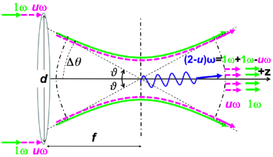
Figure 1: A quasi-parallel collision system (QPS) combining two-color laser fields with beam diameter $d$ and focal length $f$, where the incident angle $\vartheta$ is subject to $0<\vartheta\leq\Delta\theta$, which is unavoidable because of the ambiguity of the wave vectors of the incident photons due to the nature of the focused lasers. This figure is reproduced from PTEP-EXP01 with a slight modification.

A QPS can be realized conceptually by focusing a laser beam with a focusing optical component as illustrated in Fig. 1. The solid (green) laser field with photon energy $\omega$ is focused, and the center of mass system (CMS) energy between a randomly selected photon pair within the focused field is expressed as

$$E_{CMS}=2\omega\sin{\vartheta},$$ (1)

where $\vartheta$ is half of the relative incident angle of the photon pair. By adjusting the beam diameter $d$ and focal length $f$, we can control the range of possible incident angles within $\Delta\theta$, that is, the accessible range of $E_{CMS}$ in a single focusing geometry. Because $\vartheta$ can be close to zero, the QPS is in principle sensitive to pNGBs with almost zero mass. Consequently, the photon–photon scattering in the QPS is accessible to the mass range $0<m<2\omega\Delta\theta$, although the sensitivity to a lower mass range is steeply suppressed. Capturing a resonant pNGB within an $E_{CMS}$ uncertainty via an $s$-channel exchange is the first key element of this method to increase the interaction rate. The second key element is in stimulation to guide the scattering to a fixed final state. The dashed (magenta) laser beam with photon energy $u\omega$ ($0<u<1$) indicates the inducing laser field to stimulate the interaction, where the probability of generating a signal photon with energy $(2-u)\omega$ is enhanced via energy–momentum conservation in $\omega+\omega\rightarrow pNGB\rightarrow u\omega+(2-u)\omega$ by the coherent nature of the co-propagating inducing laser. The scattering probability increases in proportion to (i) the number of photons in the inducing laser and (ii) the square of the number of photons in the creation laser DEptp ; TajimaHomma ; DEapb ; DEptep . This process is kinematically similar to four-wave mixing in the context of atomic physics FWM .

Herein, we report the results of the third search by increasing the laser intensities with the upgraded experimental systems. To increase the creation laser intensity in particular, we used a Ti:Sapphire-based laser, $T^{6}$-laser at the Institute for Chemical Research at Kyoto University, which can produce a 10 TW pulse intensity at maximum peak power at a repetition rate of 5 Hz. For this upgrade, main optical components were installed in the vacuum system which consists of transport chambers and an interaction chamber separately. We mostly respected construction of the high-quality vacuum system, especially for the interaction part, which required downsizing of the optical paths and also the capability to manipulate optical components from outside these chambers. The main purpose of the present search is therefore to show the extensibility of this searching method in such a high-quality vacuum system, even if new types of background sources emerge as a result of increased laser intensities.

II Coupling-mass relation configured for the search

In order to discuss the coupling of scalar ($\phi$) or pseudoscalar ($\sigma$) fields to two photons, we introduce the following two effective Lagrangians:

$$-L_{\phi}=gM^{-1}\frac{1}{4}F_{\mu\nu}F^{\mu\nu}\phi,\hskip 10.0pt-L_{\sigma}=gM^{-1}\frac{1}{4}F_{\mu\nu}\tilde{F}^{\mu\nu}\sigma,$$ (2)

where $F^{\mu\nu}=\partial^{\mu}A^{\nu}-\partial^{\nu}A^{\mu}$ is the field strength tensor and its dual $\tilde{F}^{\mu\nu}$ is defined as $\epsilon^{\mu\nu\alpha\beta}F_{\alpha\beta}$ with the Levi-Civita symbol $\epsilon^{ijkl}$, and $g$ is a dimensionless constant while $M$ is a typical energy at which a relevant global symmetry is broken.

The scalar and pseudoscalar fields couple to the two photons differently depending on the linear polarization states of the two photons. In the photon-photon scattering process $p_{1}+p_{2}\rightarrow p_{3}+p_{4}$ in four-momentum space, when all photons are on an identical reaction plane, that is, in the case of the coplanar condition, the distinction between scalar and pseudoscalar field exchanges becomes prominent as follows. Denoting individual linear polarization states in parentheses, the non-vanishing scattering amplitudes are limited to

$$p_{1}(1)+p_{2}(1)\rightarrow p_{3}(2)+p_{4}(2)$$

$$p_{1}(1)+p_{2}(1)\rightarrow p_{3}(1)+p_{4}(1)$$ (3)

for the scalar field exchange and

$$p_{1}(1)+p_{2}(2)\rightarrow p_{3}(1)+p_{4}(2)$$

$$p_{1}(1)+p_{2}(2)\rightarrow p_{3}(2)+p_{4}(1)$$ (4)

for the pseudoscalar field exchange, where swaps between (1) and (2) give the same scattering amplitudes, respectively.

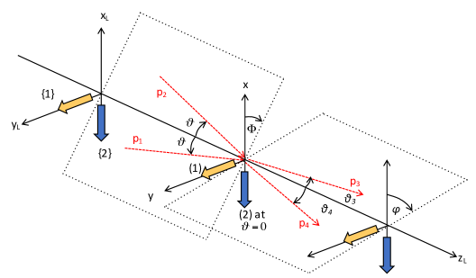
Figure 2: Definitions of linear polarization directions and rotation angles in focused collision geometry. This figure is reproduced from PTEP-EXP01 with a slight modification.

While this coplanar condition is always satisfied in CMS, it is not true in the case of QPS as illustrated in Fig.2, where the $\vec{p}_{1}-\vec{p}_{2}$ plane and the $\vec{p}_{3}-\vec{p}_{4}$ plane may differ from the $x_{L}-z_{L}$ plane in the laboratory coordinates. We define experimental linear polarization states {1} and {2} by mapping them along $y_{L}$ and $x_{L}$ axes, respectively. We then define rotation angles of these reaction planes as $\Phi$ and $\varphi$ for initial and final state photon pairs, respectively, with respected to the $x_{L}-z_{L}$ plane.

In this search, indeed, we will assign the P-polarized state of the creation laser to {1} state and the S-polarized state of the inducing laser to {2} state, because the orthogonal combination of P- and S-polarization states is very effective to suppress the known atomic four-wave mixing process in the residual gas FWM ; PTEP-EXP01 .

For a given set of fixed laboratory polarization directions {1} and {2}, we have introduced an axially asymmetric factor ${\cal F}_{abcd}$ with linear polarization states $ab$ and $cd$ for the initial and final state photon pairs, respectively, by fixing $\Phi=0$ for scalar and pseudoscalar cases, respectively DEptep . If there is no inducing field in the final state, $\vec{p}_{3}-\vec{p}_{4}$ planes rotate around the $z_{L}$ axis symmetrically resulting in the axial symmetric factor of $2\pi$ due to the solid angle integration of signal photons. However, since we induce $p_{3}$ photons as the signal by supplying the polarization-fixed coherent $p_{4}$ field in the search, the $\vec{p}_{3}-\vec{p}_{4}$ plane rotation factor deviates from $2\pi$ depending on types of exchanged fields. So the ${\cal F}$-factor corresponds to the replacement of the symmetric solid angle integral.

In addition we have further introduced an incident plane rotation factor ${\cal G}_{ab}$ in QPS PTEP-EXP01 , because theoretically introduced $\vec{p}_{1}-\vec{p}_{2}$ planes are independent of the experimentally introduced $x_{L}-z_{L}$ plane based on {1} and {2} states of creation and inducing laser fields, respectively. Thanks to this situation, even if the polarization direction of the creation laser field is fixed at {1} state in the laboratory coordinates, the searching system can also be sensitive to the pseudoscalar field exchange through the rotation of the $\vec{p}_{1}-\vec{p}_{2}$ plane. The ${\cal G}$-factor corresponds to an averaged correction factor with respect to the case with $\Phi=0$ by taking possible rotation angles over $\Phi=0\sim 2\pi$.

In this search we thus focus on the following scattering processes in the same way as the previous publication PTEP-EXP01 :

$$p_{1}(1)+p_{2}(1)\rightarrow p_{3}(2)+p_{4}(2)$$ (5)

with the assumption of the scalar field exchange and

$$p_{1}(1)+p_{2}(2)\rightarrow p_{3}(1)+p_{4}(2)$$ (6)

with that of the pseudoscalar field exchange.

For given parameters for the pulsed lasers and optical components, the coupling strength $g/M$ is related to the yield $\mathcal{Y}$ based on Eq.(26) in Appendix herein, namely, the number of $p_{3}$ photons, via

$$\frac{g}{M[\mbox{eV}]}=2^{1/4}8\pi^{2}\sqrt{\frac{\mathcal{Y}\omega^{3}_{c}[\rm{eV}]}{\left(\frac{\lambda_{c}}{c\tau_{c}}\right)\left(\frac{\tau_{c}}{\tau_{i}}\right)\left(\frac{f}{d_{c}}\right)^{3}\frac{\pi}{4}\left(\frac{d_{c}}{d_{i}}\right)^{2}\frac{(\overline{u}-\underline{u})^{2}}{\overline{u}\underline{u}}\mathcal{W}\mathcal{G}_{ab}\mathcal{F}_{abcd}C_{mb}{N_{c}}^{2}N_{i}}}m^{-5/2}[\rm{eV}],$$ (7)

where the subscripts $c$ and $i$ denote the creation and inducing lasers, respectively. This relation is almost the same as the one used for the second search PTEP-EXP01 except for the condition that the beam diameters of the creation and inducing lasers are non-negligibly different in the present search, so the common diameter parameter for both beams cannot be assigned. The relevant modifications are summarized in Appendix herein, while all the other details are given in the appendices of the previous searches PTEP-EXP00 ; PTEP-EXP01 . The individual parameters are then summarized as follows: $\omega_{c}$ is the incident photon energy of the creation laser, $\lambda_{c,i}$ are the wavelengths of the two lasers, $\tau_{c,i}$ are the pulse durations, $f$ is the common focal length, $d_{c,i}$ are the beam diameters, $\mathcal{W}$ is the numerical factor relevant to the weighted integral of a Breit–Wigner resonance, $\overline{u}$ and $\underline{u}$ are the upper and lower values, respectively, of $u$ determined by the spectrum width of $\omega_{i}$ based on $u\equiv\omega_{i}/\omega_{c}$, $C_{mb}$ is the combinatorial factor originating from selecting a pair of photons among multimode frequency states of the creation laser, and $N_{c,i}$ are the mean numbers of photons per laser pulse.

III Experimental setup

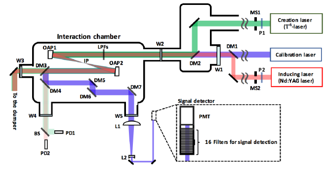
Figure 3: Schematic of the searching system contained in a beam transport chamber and an interaction chamber designed to achieve $10^{-8}$ Pa.

The search was performed with the setup illustrated in Fig. 3. A Ti:Sapphire pulsed laser with a central wavelength of 808 nm and a duration of 34 fs was used as the creation field, and an Nd:YAG pulsed laser with a central wavelength of 1064 nm and a duration of 9 ns was used as the inducing field. The linear polarization state of the creation laser was produced at P1 before the pulse compression. P1 consisted of 30 synthetic quartz plates tilted at Brewster’s angle to transmit only p-polarized waves. The measured extinction ratio with the full energy shots was approximately 1000 (p-pol.) : 1 (s-pol.). The linear polarization state of the inducing laser was produced at P2 with a commercial polarization beam splitter with an extinction ratio 200 (p-pol) : 1 (s-pol.) and then the p-polarized waves were converted into s-polarized waves by a periscope. The s-polarized waves can be further rotated by a half-wave plate for the systematic studies. The creation and inducing lasers with beam diameters of 38 mm and 16 mm, respectively, were combined by a dichroic mirror (DM2). A 6-mm-thick window (W2) separated the vacuum systems between the interaction point (IP) and the upstream transport parts. The combined beam was thus focused into the higher-quality vacuum part inside the interaction chamber after penetrating through W2. An off-axial parabolic mirror (OAP1) with a focal length of 279.1 mm was used for the focusing. Signal photons appeared only when spatiotemporal synchronization was achieved between the two pulsed beams at IP. Background photons with the same wavelength as the signal ones generated along the optical path before OAP1 were removed by five long-pass filters (LPFs) that cut the signal wavelengths but transmitted the creation and inducing wavelengths in advance of OAP1.

Images of the beam profiles on the focal plane were transferred to a CCD camera located outside the interaction chamber by an infinity-corrected optical system. The camera recorded the number of beam photons per pixel with a spatial resolution of 0.3 $\mu$m. The physical image size was calibrated by transferring a mesh image located at IP whose physical size was known a priori. The spatial synchronization of the two beams was ensured by adjusting optical components inside the transport chambers for the creation laser and those outside the chambers for the inducing laser so that the centers of the focal spots of the two beams coincided. The focal-spot images of the creation and inducing lasers used for the search are shown in Fig. 4. A beam diameter at IP is defined as the full width at half maximum (FWHM) of the 2-D Gaussian function fitted to a focal image. The measured diameters were $\sigma_{x}=10~{}\mu$m and $\sigma_{y}=7~{}\mu$m in the horizontal $x$ and vertical $y$ directions for the creation laser, while those of the inducing laser were $\sigma_{x}=23~{}\mu$m and $\sigma_{y}=19~{}\mu$m.

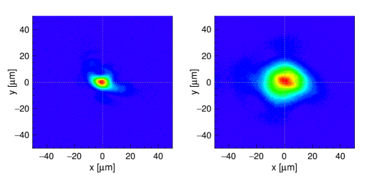
Figure 4: Beam profiles of creation (left) and inducing (right) lasers at IP captured by a common CCD camera.

With the central wavelengths $\lambda_{c}$ and $\lambda_{i}$ for the creation and inducing lasers, respectively, the central wavelength $\lambda_{s}$ of the signal is defined via energy conservation as

$$\lambda_{s}=\left(\frac{2}{\lambda_{c}}-\frac{1}{\lambda_{i}}\right)^{-1}=651\hskip 3.0pt\mbox{nm},$$ (8)

which is close to the 633 nm wavelength of a He:Ne laser. Thus, the He:Ne laser was used to trace the signal trajectory down to the signal sensor combined with the inducing laser by DM1 and then with the creation laser by DM2. This calibration laser was used to align all the optical components inside the interaction chamber and to evaluate the detector acceptance from IP to the sensor surface.

OAP1 and OAP2 were identical mirrors subtending IP at the same focal length. The combined beam was focused by OAP1 and then collected by OAP2, which restored the plane waves. The custom-made dichroic mirrors DM3 through DM7, each of which reflected 651 nm with 99% while transmitting around 806 nm with 99% and 1064 nm with 95 %, discriminated the signal photons from the residual creation and inducing laser beams. The combined pulses that had passed through DM4 were measured by photodiodes (PD1, PD2) with $\sim 40$ ps time-resolution to monitor the stability of the pulse energies and to adjust the time synchronization between the creation and inducing laser pulses.

As a signal detector, we used an R7400-01 single-photon-countable photomultiplier tube (PMT) manufactured by HAMAMATSU which has a falling time resolution of 0.75 ns. In order for the detection system to be sensitive only to signal photons between 610 and 690 nm, the PMT was installed after an LPF transmitting above 610 nm and three types of band-pass filters transmitting 570–800 nm, 500–930 nm, and 450–690 nm to remove residual photons from the intense incident lasers

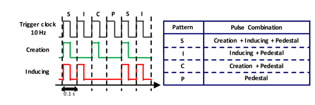
Figure 5: Four consecutive trigger patterns.

We acquired waveform data of analog currents from the PMT and the two PDs using a waveform digitizer triggered with a basic 10 Hz trigger to which both the creation and inducing laser injections were synchronized as shown in Fig. 5. Two mechanical shutters reduced the injection rate of the creation laser down to equi-interval 5 Hz and that of the inducing laser to non-equi-interval 5 Hz for waveform analysis as indicated in Fig. 5. The two beams were injected with different timing patterns so that the waveform data could be recorded with the following four consecutive trigger patterns with equal statistics: (i) both beams were incident ”S”, (ii) only the inducing laser was incident ”I”, (iii) only the creation laser was incident ”C”, and (iv) neither beam was incident ”P”.

IV Measurement of four-wave mixing process in residual gas

The observed number of photons was estimated by analyzing the waveform data from the PMT. An individual waveform consisted of 1000 sampling data points within a 500 ns time window. Figure 6 shows an example of waveform data in which a peak is identified.

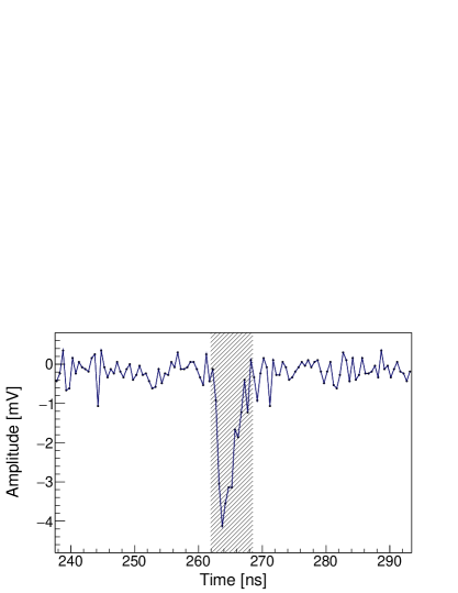
Figure 6: Waveform data sample including a peak. The shaded area shows the integral range used to evaluate the charge sum of the peak structure.

Negative peaks were identified with a peak finder applying the same algorithm as that in the previous search PTEP-EXP01 . We then calculated the charge sums in the peak structures. The charge sums in the peak structures were converted to the number of photons by dividing by the measured single-photon equivalent charge.

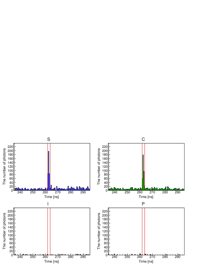
Figure 7: Arrival time distributions of the number of observed photons in the case of the P-pol.(creation) + P-pol.(inducing) combination for individual trigger patterns at 10 Pa. Individual time windows in which signal photons are expected to be detected are indicated with the two red lines.

Four-wave mixing photons are expected to be caused by residual gases in the interaction chamber as a background source. However, this photon source can be used as a calibration source to assure the spatiotemporal synchronization of the creation and inducing laser pulses. To quantify the number of background photons, we measured the pressure dependence of the number of four-wave mixing photons when the linear polarization directions of the creation and inducing lasers were parallel to enhance the atomic four-wave mixing process. Figure 7 shows the arrival time distribution in units of the number of photons at 10 Pa for each of the four trigger patterns. There is a peak structure in not only trigger pattern S but also in pattern C. The background photons in trigger pattern C are expected to originate from plasma creation by the ionization of the residual atoms when the high-intensity creation laser is focused at IP. This phenomenon was not observed in the previous search PTEP-EXP01 because of the lower intensity of the creation laser field.

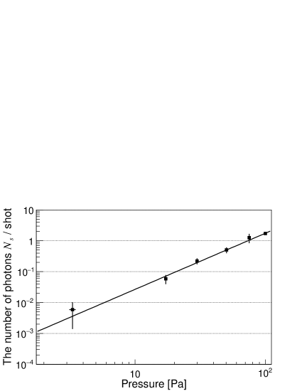
Figure 8: Pressure dependence of the number of four-wave mixing photons per shot from the residual atoms inside the interaction chamber when the two beams with the same linear polarization directions, P-pol.(creation) + P-pol.(inducing), are focused.

The number of four-wave mixing photons, $N_{S}$, was then evaluated from

$$N_{S}=n_{S}-n_{C}-n_{I}+n_{P},$$ (9)

where $n_{T}$ is the number of photons for a trigger pattern $T$ entering the time window 262.5–264 ns, which is consistent with the signal generation timing. Figure 8 shows the pressure dependence of the number of signal photons per shot, which was fitted with

$$N_{S}/shot=a{\cal P}^{b},$$ (10)

where $a$ and $b$ are fitting parameters and ${\cal P}$ is the pressure. The error bars include the error propagation in the subtraction process based on statistical fluctuations of the reconstructed number of photons and uncertainties of focal-point stability during a run period. The latter fluctuations were evaluated from overlaps between the two laser profiles measured by the common CCD camera which was sensitive to both wavelengths. The overlap factor $O$ is defined as

$$O\equiv\sum_{x}^{c}\sum_{y}^{c}N^{2}_{c}(x,y)N_{i}(x,y),$$ (11)

where subscripts $c$ and $i$ indicate the creation and inducing lasers, respectively and $N(x,y)$ is the local intensity per CCD pixel of the monitor camera. The summations were over the area framed by FWHM of the creation laser intensity profile. Fluctuations of the overlap factors were then estimated as

$$\delta N_{S}=\left|N_{S}\frac{O_{I}-O_{F}}{O_{I}+O_{F}}\right|,$$ (12)

where $O_{I,F}$ are the overlap factors at the beginning and end, respectively, of a unit run period during 1200 s, and deviations with respect to the mean overlap factor $(O_{I}+O_{F})/2$ were calculated. The value of $b=1.82\pm 0.14$ from the fitting results is close to the expected behavior $N_{S}\propto{\cal P}^{2}$ in atomic four-wave mixing processes FWM ; PTEP-EXP01 .

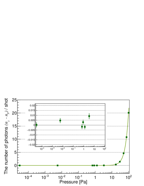
Figure 9: Pressure dependence of the number of photons, $n_{c}-n_{p}$, per shot when only linearly polarized creation laser pulses are focused in trigger pattern C. The errors are statistical errors associated with subtracting side-band distributions from the number of photons within the signal generation timing window. Data points were fitted with $a{\cal P}^{b}+c$, resulting in $b=2.22\pm 0.01$ and $c=-6.58\times 10^{-6}\pm 1.05\times 10^{-3}$. The inset figure zooms the constant points.

A notable difference from our previous publication PTEP-EXP01 was that signal-like photons were indeed produced even in trigger pattern C. Figure 9 shows the number of photons, $n_{c}-n_{p}$, in trigger pattern C within the signal timing window after subtracting the side-band background photons from the peak part as a function of pressure. This indicates that $n_{c}-n_{p}$ scales with ${\cal P}^{2.2}$ and reaches zero within the statistical uncertainty below 1 Pa. Because $n_{c}-n_{p}$ is strongly pressure dependent, we conclude that this background source is generated from IP but different from the conventional four-wave mixing process because it does not require the inducing laser to produce the same frequency as that of four-wave mixing. Creation of a plasma state at IP by the higher-power creation laser might explain the broad-band emissions, though this is not directly relevant to the present search because we can subtract trigger pattern C from pattern S.

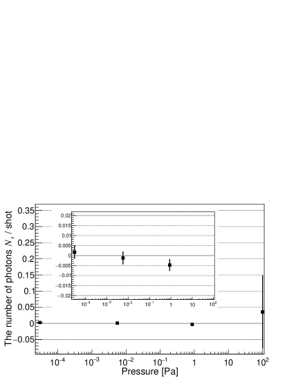
Figure 10: Pressure independence of the number of four-wave mixing photons per shot from the residual atoms inside the interaction chamber when the two beams with the orthogonal linear polarization combination, P-pol.(creation) + S-pol.(inducing), are focused.

V Search for four-wave mixing signals in vacuum

We searched for scalar- and pseudoscalar-type resonance states at a vacuum pressure of $3.7\times 10^{-5}$ Pa by combining P-pol. for the creation pulsed laser and S-pol. for the inducing pulsed laser.

When the polarization directions of the two beams were orthogonal, P-pol.(creation) + S-pol.(inducing), counting the number of four-wave mixing photons in the similar pressure range to that of the P-pol.(creation) + P-pol.(inducing) case was rather difficult because the number of photons in trigger pattern C was considerable and the subtraction from trigger pattern S was dominated by the statistical uncertainty. However, we know that the parallel case dominates the orthogonal case at a higher pressure range above $10^{2}$ Pa  PTEP-EXP01 . Thus, the pressure dependence in Fig. 8 can give an upper limit on the number of photons from the atomic four-wave mixing process even without the measured pressure dependence for the orthogonal case, which is the actual searching configuration as discussed in Section II. Figure 10 shows the independence of the number of photons with respect to pressure values in the case of the orthogonal polarization combination at a much lower pressure range compared to Fig. 8. Although the subtraction error at around several Pa is much larger due to finite background photons seen in trigger pattern C and S, the inset figure zooming the points below 1 Pa indicates that the observed numbers of photons are consistent with null over five orders of magnitude in the pressure values.

The upper limit on the expected number of background photons per shot (efficiency-uncorrected) caused by residual gases at $3.7\times 10^{-5}$ Pa was evaluated by extrapolating with Eq. (10) based on the parallel polarization combination case as follows:

$$N_{gas}/shot<2.2\times 10^{-11},$$ (13)

where the upper limit was estimated by taking the maximum value based on the fitting error on the parameter $b$. Therefore, in the case of the orthogonal polarization combination, the expected number of background photons caused by the residual atoms is below unity as long as the total statistic is below $10^{11}$ shots.

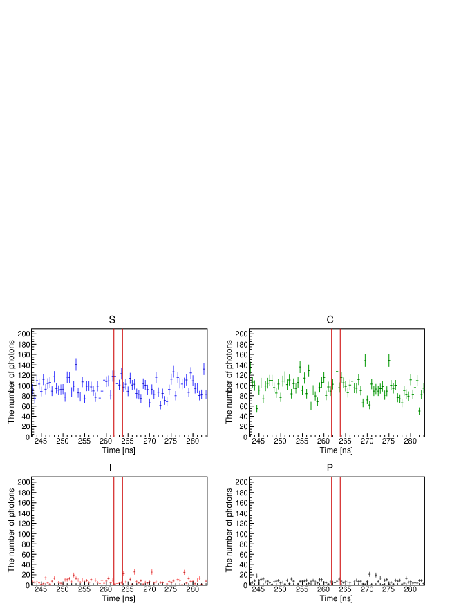
Figure 11: Arrival time distributions of detected photons at $3.7\times 10^{-5}$ Pa for trigger patterns S, C, I, and P with the P-pol.(creation) + S-pol.(inducing) combination.

Figure 11 shows the arrival time distributions of detected photons at $3.7\times 10^{-5}$ Pa for individual trigger patterns with the total number of shots in trigger pattern S defined as $W_{S}\equiv 4.2\times 10^{4}$ in the case of the orthogonal polarization combination, P-pol.(creation) and S-pol.(inducing). Figure 12 shows the arrival time distribution of the number of photons obtained by applying Eq. (9) to the other timing windows including that of the four-wave mixing signal enclosed by the two red lines. The total number of four-wave mixing photons within the signal generation timing in the quasi-vacuum state was obtained as

$$N_{S}=5.4\pm 30.7(\rm{stat.})\pm 25.1(\rm{syst.I})\pm 10.1(\rm{syst.II})\pm 0.9(\rm{syst.III}).$$ (14)

Systematic error I is the uncertainty caused by the number of photons present outside the time window of the signal. This was estimated by measuring the root-mean-square of the number of photon-like signals excluding the signal window. Systematic error II originates from fluctuations of the overlap factors between the focal spots of the creation and inducing lasers as discussed in Section IV. We emphasize that Eq.(11) includes fluctuations of the numbers of photons, $N_{c,i}$, observed at the focal spots, namely, fluctuations of beam energies during a run period together with the position dependence, namely, pointing fluctuations. The absolute values of laser pulse energies for the creation and inducing lasers were $101\pm 4$ $\mu$J and $300\pm 5$ $\mu$J, respectively, at the beginning of the first run, while they were $98\pm 4$ $\mu$J and $303\pm 5$ $\mu$J, respectively, at the end of the final run. So the absolute pulse energies of the two lasers were quite stable over the entire data taking period for 40 hours. This overlap factor reflects the nature of four-wave mixing on the cubic intensity dependence. Systematic error III is an error caused by the threshold value used for the peak finding. This was calculated as two standard deviation assuming that the number of photon-like signals obtained by varying $V_{threshold}$ from $-1.2$ to $-1.4$ mV follows a uniform distribution.

VI Excluded coupling-mass regions for scalar and pseudoscalar fields

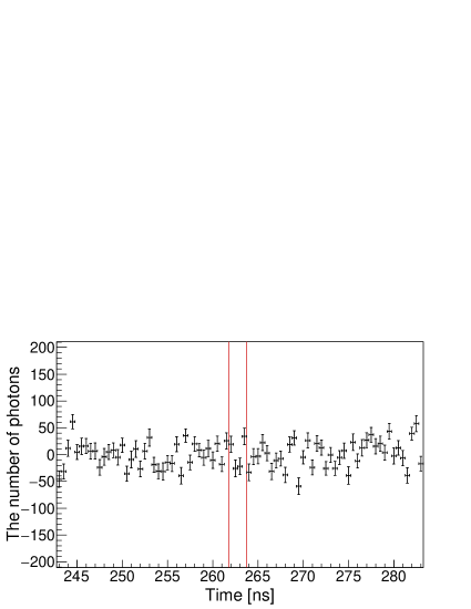
Figure 12: Arrival time distribution of the number of photons obtained by applying Eq. (9) to the other timing windows including that of the four-wave mixing signal enclosed by the two red lines at $3.7\times 10^{-5}$ Pa in the case of the orthogonal polarization combination, P-pol.(creation) and S-pol.(inducing).

Table 1: Experimental parameters to set exclusion regions for the coupling-mass relations. $\mathcal{G}^{sc}_{11}$ and $\mathcal{G}^{ps}_{12}$ are averaging factors by the incident reaction plane rotation for scalar and pseudoscalar field exchanges, respectively. The evaluation of $\mathcal{G}$ is discussed in the appendix of the previous search PTEP-EXP01 . $\mathcal{F}^{sc}_{1122}$ and $\mathcal{F}^{ps}_{1212}$ are axially asymmetric factors for scalar and pseudoscalar field exchanges, respectively, as explained in the appendix of DEptep . Note that the effective $N_{i}$ is deduced from the overlap between the measured focal images of the inducing and creation lasers within the area framed by $\pm 3$ standard deviation in the Gaussian-like intensity profile of the creation laser.

Parameter	Value
Total number of shots in trigger pattern $S$, $W_{S}$	$4.2\times 10^{4}$ shots
Center of wavelength of creation laser $\lambda_{c}$	808 nm
Relative line width of creation laser ($\delta\omega_{c}/<\omega_{c}>)$	$2.0\times 10^{-2}$
Center of wavelength of inducing laser $\lambda_{i}$	1064 nm
Relative line width of inducing laser ($\delta\omega_{i}/<\omega_{i}>)$	$1.0\times 10^{-4}$
Duration time of creation laser pulse per injection $\tau_{c}$	34 fs
Duration time of inducing laser pulse per injection $\tau_{i}$	9 ns
Creation laser energy per $\tau_{c}$	101 $\pm$ 4 $\mu$J
Inducing laser energy per $\tau_{i}$	142 $\pm$ 2 $\mu$J
Focal length of off-axis parabolic mirror $f$	279.1 mm
Beam diameter of creation laser beam $d_{c}$	38 $\pm$ 0.8 mm
Beam diameter of inducing laser beam $d_{i}$	16 $\pm$ 0.3 mm
Upper mass range given by $\vartheta<\Delta\theta$	0.21 eV
$u=\omega_{i}/\omega_{c}$	0.76
Incident-plane-rotation averaging factor $\mathcal{G}_{ab}$	$\mathcal{G}^{sc}_{11}$=19/32
	$\mathcal{G}^{ps}_{12}$=1/2
Axially asymmetric factor $\mathcal{F}_{abcd}$	$\mathcal{F}^{sc}_{1122}$=19.4
	$\mathcal{F}^{ps}_{1212}$=19.2
Combinatorial factor in luminosity $C_{mb}$	1/2
Single-photon detection efficiency $\epsilon_{D}$	1.4 $\pm$ 0.1 %
Efficiency of optical path from IP to PMT $\epsilon_{opt}$	32.6 $\pm$ 4.0 %
$\delta{N}_{s}$	40.9

No statistically significant four-wave mixing photons in the quasi-vacuum state were observed in this search from the result in (14). We thus set the exclusion regions on the coupling-mass relation by assuming scalar and pseudoscalar fields based on the parameter values summarized in Tab.1.

First, the upper limit on the sensitive mass range is estimated as

$$m<2\omega_{c}\sin\Delta\theta\sim 2\omega_{c}\frac{d_{c}}{2f}=0.21\mbox{~{}eV}$$ (15)

based on values in Tab.1, where $\Delta\theta$ is defined by the focal length $f$ and beam diameter $d$ of the creation laser in Fig. 1 and $\vartheta$ varies from zero to $\Delta\theta$.

The efficiency-corrected number of four-wave mixing photons, $\mathcal{N}_{S}$, was evaluated from the following relation with the relevant experimental parameters:

$$\mathcal{N}_{S}=\frac{N_{S}}{\epsilon_{opt}\epsilon_{D}},$$ (16)

where $\epsilon_{opt}$ is the acceptance factor for signal photons to propagate from IP through several optical components, and $\epsilon_{D}$ is the detection efficiency of the PMT due mainly to the quantum efficiency of the photocathode when a single photon enters. $\epsilon_{opt}$ includes the inefficiencies from IP down to the actual location of the PMT, namely, those of OAP2, DM3-DM7, W5, L1-L2, and the transmittance of the 16 wave filters in front of the PMT. This factor was evaluated by taking the ratio between the calibration beam energy at the focal point and that at the detection point. The energy ratio was measured based on the intensity distributions at the common camera. In advance of the search, $\epsilon_{D}$ was measured with 532 nm laser pulses. We corrected the difference of the quantum efficiencies between 532 nm and 651 nm based on the relative quantum efficiencies provided by the HAMAMATSU specification sheet.

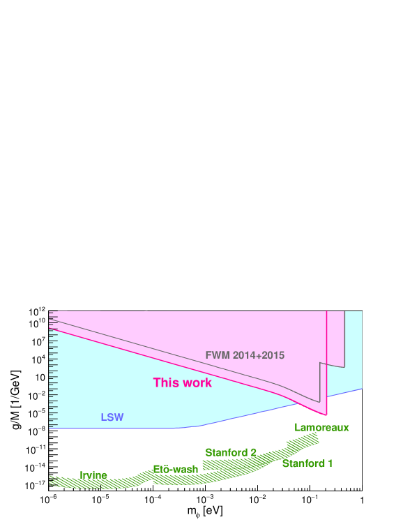
Figure 13: Excluded regions in the coupling-mass relation for scalar-type fields ($\phi$). The magenta area represents the excluded region by our method, ”Four-Wave Mixing (FWM)”. The thick magenta line is the new limit by this search, while the gray line is the merged result from previous searches PTEP-EXP00 ; PTEP-EXP01 . The light blue area is the excluded region for scalar fields by the ”Light Shining through a Wall (LSW)” experiments (OSQAR osqar and ALPS alps ) with simplification of the sine-function part to unity above $10^{-3}$ eV for drawing purpose. The green shaded areas show regions excluded by non-Newtonian force searches by torsion-balance experiments ”Irvine” Irvine , ”Eto-wash” Eto-wash , ”Stanford1” Stanford1 , ”Stanford2” Stanford2 and Casimir force measurement ”Lamoreaux” Lamoreaux .

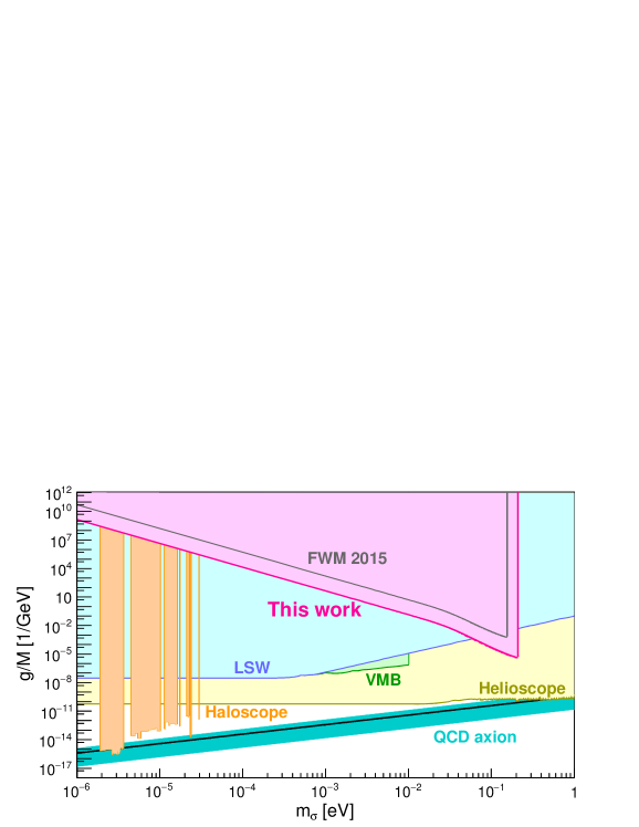
Figure 14: Excluded regions in the coupling-mass relation for pseudoscalar-type fields ($\sigma$). This search based on FWM excludes the magenta area, while the gray line is the limit by the previous search PTEP-EXP01 . The cyan band indicates the expected coupling-mass relation of the QCD axion predicted by the KSVZ model KSVZ1 ; KSVZ2 with $|E/N-1.95|$ in the range 0.07–7. The case of $E/N=0$ is also shown by the black solid line. The light blue area indicates the excluded region by LSW experiments (OSQAR osqar and ALPS alps ) for the pseudoscalar search. The green area represents the result from the ”Vacuum Magnetic Birefringence (VMB)” experiment (PVLAS pv ). The yellow area shows the exclusion limit from the ”Helioscope” experiment (CAST cast ). The orange areas indicate excluded regions from ”Haloscope” experiments (ADMX admx , RBF rbf , UF uf and HAYSTAC haystac ).

The upper limits on the coupling-mass relation at a 95 % confidence level were obtained based on the null hypothesis that the fluctuations of the number of signal photons follow Gaussian distributions whose expectation value, $\mu$, is zero for the given total number of shots, $W_{S}=4.2\times 10^{4}$. This null hypothesis is justified. First, the expectation value based on the unique standard model process, that is, the QED photon-photon scattering process is negligibly small at $E_{cms}<1$ eV PTEPGG even if we add the stimulation effect PTEP17 for the given shot statistics. Second, as discussed with inequality Eq. (13), the expectation value due to atomic processes in the residual gas is well below unity. Therefore, the background source is limited to only noises in the experimental environment. The systematic error I is the dominant component of the systematic errors. This was estimated by measuring the root-mean-square of the number of photon-like signals excluding the signal window. In fact, the measured $N_{s}$ distribution excluding the signal time window follows almost a perfect Gaussian distribution around its central value, though the central value itself has no specific meaning with respect to the signal timing window. Since the distribution is symmetric around the central value, a Gaussian distribution can be supported from the measurement whatever the physics behind it is. The Gaussian distribution is also deduced from the principle point of view. What we measure is accidentally incident photon-like waveforms in arbitrary time window ($e.g.$ thermal noises, ambient photons from lasers and not from lasers, electric noises, and so forth) which should follow binomial distributions if the incident probabilities are individually constant over the measuring time. Although the incident probabilities are quite low, the expectation values of background photon-like signals per time bin over the data acquisition time are around 100 as seen in trigger pattern S and C in Fig.11. Therefore, we may expect that the numbers of background photons per time bin can be approximated as Gaussian distributions because the expectation value is large enough. $N_{s}$ then eventually corresponds to subtractions between these Gaussian distributions. We thus assume that the Gaussian distribution is the most natural null hypothesis in our search. In order to set a confidence level $1-\alpha$ to exclude the null hypothesis, we assign the acceptance-uncorrected uncertainty $\delta N_{S}$ which was evaluated as the quadratic sum of statistical and systematic errors in Eq. (14) as the one standard deviation $\sigma$ to the following Gaussian kernel:

$$1-\alpha=\frac{1}{\sqrt{2\pi}\sigma}\int^{\mu+\delta}_{\mu-\delta}e^{-(x-\mu)^{2}/(2\sigma^{2})}dx=\mbox{erf}\left(\frac{\delta}{\sqrt{2}\sigma}\right),$$ (17)

where $\mu=0$ and $N_{S}$ corresponds to the estimator $x$ in our case. In order to give a confidence level of 95 % in this analysis, we apply $2\alpha=0.05$ with $\delta=2.24\sigma$ where we set a one-sided upper limit by excluding above $x+\delta$ PDGstatistics . The upper limit of the signal yield to be compared to the theoretical calculation, namely, $\mathcal{Y}$, was then evaluated as

$$\mathcal{Y}=\frac{2.24\delta{N}_{S}}{\epsilon_{opt}\epsilon_{D}W_{S}}.$$ (18)

Based on the coupling-mass relations in Eq. (7), Figs. 13 and 14 show the obtained exclusion limits for scalar and pseudoscalar fields, respectively, at a 95 % confidence level.

VII Conclusions

We performed an extended search for scalar and pseudoscalar fields via four-wave mixing by focusing two-color pulsed lasers, namely, 0.10 mJ/34 fs at 808 nm and 0.14 mJ/9 ns at 1064 nm. The observed number of four-wave mixing photons in the quasi-vacuum state at $3.7\times 10^{-5}$ Pa was $5.4\pm 30.7(\rm{stat.})\pm 25.1(\rm{syst.I})\pm 10.1(\rm{syst.II})\pm 0.9(\rm{syst.III})$. We thus conclude that no significant four-wave mixing signal was observed in this search. The expected number of four-wave mixing photons from the residual gas is sufficiently small based on the upper limit from the measurement of the pressure dependence. With respect to an assumption that uncertainties are dominated by systematic fluctuations around the zero expectation value following the Gaussian distribution, we provided the upper limits on the coupling-mass relations for scalar and pseudoscalar fields at a 95 % confidence level in the mass range below 0.21 eV, respectively. The upper limits on the coupling at $m=0.21$ eV were obtained as $4.6\times 10^{-6}$ GeV^-1 and $5.1\times 10^{-6}$ GeV^-1 for scalar and pseudoscalar fields, respectively.

VIII Discussion and future prospect

For this extended search, we upgraded the searching system so that it can store multiple dichroic mirrors to select feeble signal photons among a huge number of background laser fields co-linearly propagating with the signal photons in the high-quality vacuum system. We prioritized construction of the high-quality vacuum system over rapid increase of the creation laser intensity, which is designed to achieve $10^{-8}$ Pa if a metal shield is installed for the lid contact, by introducing the entrance window (W2 in Fig. 3) in the interaction chamber to completely decouple the upstream transport vacuum system where the pressure is much higher. However, this window material indeed became an obstacle against drastically increasing the laser intensity, because high-intensity laser fields must penetrate the window through which a new background source was created in addition to the residual atoms around IP. Therefore, the intensity improvement for the creation laser from the previously published search PTEP-EXP01 was rather moderate in the present search. In this search, however, we have shown clearly that the null result can be obtained with the current searching method, and we succeeded in measuring the pressure scaling of the atomic four-wave mixing process and also another plasma-like phenomenon down to $\sim 1$ Pa. For the next upgraded search, we thus plan to eliminate this window. Instead, a differential pumping system will be inserted between the transport vacuum system and the interaction chamber. Therefore, we may expect that we can drastically improve the sensitivity with $\sim 10^{3}$ times higher creation laser intensity available at the $T^{6}$-laser system in the upgraded system.

Appendix: modifications of the coupling-mass relation due to the beam diameter difference

We basically use the coupling-mass relation that was used for the previous searches PTEP-EXP00 ; PTEP-EXP01 , where a common beam diameter was assumed for both the creation $(c)$ and inducing $(i)$ laser beams. However, here we slightly modify the parametrization by taking different beam diameters $d_{c}$ and $d_{i}$ into account. With respect to equations for relevant parameter used in the Appendix of PTEP-EXP00 , we put superscript${~{}}^{*}$ for the modified parameter notations as follows.

For the density factor for the creation beam, namely, ${\mathcal{D}}_{c}$ in Eq. (A29), we have

$${\mathcal{D}}_{c} = \int^{0}_{-f/c}dt\int^{\infty}_{-\infty}dx\int^{\infty}_{-\infty}dy\int^{\infty}_{-\infty}dz{\rho_{c}}^{2}(x,y,z,t)$$ (19)

$$= \frac{N^{2}_{c}}{\sqrt{2\pi}}\frac{1}{\pi{w_{0}}^{2}}\frac{1}{c\tau_{c}}\frac{z_{R}}{c}\left[\tan^{-1}\left(\frac{f}{z_{R}}\right)\right]$$

$\rightarrow$

$${\mathcal{D}}^{*}_{c} = \int^{0}_{-Z_{R}/c}dt\int^{\infty}_{-\infty}dx\int^{\infty}_{-\infty}dy\int^{\infty}_{-\infty}dz{\rho_{c}}^{2}(x,y,z,t)$$ (20)

$$= \frac{N^{2}_{c}}{\sqrt{2\pi}}\frac{1}{\pi{w_{0}}^{2}}\frac{1}{c\tau_{c}}\frac{z_{R}}{c}\left[\frac{\pi}{4}\right],$$

where we reduce the range of time integration from $-f/c\sim 0$ to $-Z_{R}\sim 0$ with focal length $f$ and Rayleigh length $z_{R}$, because the effect of the diameter mismatch on the overlap between the creation and the inducing lasers is expected to be larger near the surface of the focusing mirror. We thus restrict the signal generation range only in the vicinity of the focal point.

For the inducible acceptance factor ${\mathcal{A}}_{i}$ in Eq. (A32), we have

$${\mathcal{A}}_{i}\sim 4\delta{\mathcal{U}}\left(\frac{\vartheta_{r}}{\Delta\theta}\right)^{2}$$ (21)

$\rightarrow$

$${\mathcal{A}}^{*}_{i}\sim 4\delta{\mathcal{U}}\left(\frac{\vartheta_{r}}{\Delta\theta_{4}}\right)^{2}=\left(\frac{\Delta\theta}{\Delta\theta_{4}}\right)^{2}4\delta{\mathcal{U}}\left(\frac{\vartheta_{r}}{\Delta\theta}\right)^{2}=\left(\frac{d_{c}}{d_{i}}\right)^{2}4\delta{\mathcal{U}}\left(\frac{\vartheta_{r}}{\Delta\theta}\right)^{2},$$ (22)

where the approximation $\Delta\theta_{4}\sim\Delta\theta$ is no longer used because the beam diameters are not common while the focal length $f$ is common.

For the overall density factor ${\mathcal{D}}_{c+i}$ including the inducing laser effect in Eq. (A34), we have

$${\mathcal{D}}_{c+i} \sim C_{mb}\frac{N^{2}_{c}}{\sqrt{2\pi}}\frac{1}{\pi{w_{0}}^{2}}\frac{1}{c\tau_{c}}\frac{z_{R}}{c}\left[\tan^{-1}\left(\frac{f}{z_{R}}\right)\right]4\delta{\mathcal{U}}\left(\frac{\vartheta_{r}}{\Delta\theta}\right)^{2}\left(\frac{\tau_{c}}{\tau_{i}}\right)N_{i}$$ (23)

$\rightarrow$

$${\mathcal{D}}^{*}_{c+i} \sim C_{mb}\frac{N^{2}_{c}}{\sqrt{2\pi}}\frac{1}{\pi{w_{0}}^{2}}\frac{1}{c\tau_{c}}\frac{z_{R}}{c}\left[\frac{\pi}{4}\left(\frac{d_{c}}{d_{i}}\right)^{2}\right]4\delta{\mathcal{U}}\left(\frac{\vartheta_{r}}{\Delta\theta}\right)^{2}\left(\frac{\tau_{c}}{\tau_{i}}\right)N_{i}.$$ (24)

For the resultant signal yield ${\mathcal{Y}}$ in Eq. (A35), we have

$${\mathcal{Y}} = {\mathcal{D}}_{c+i}\overline{\Sigma}$$ (25)

$$\sim \frac{1}{64\sqrt{2}\pi^{4}}\left(\frac{\lambda_{c}}{c\tau_{c}}\right)\left(\frac{\tau_{c}}{\tau_{i}}\right)\left(\frac{f}{d}\right)^{3}\left[\tan^{-1}\left(\frac{\pi d^{2}}{4\ f\lambda_{c}}\right)\right]\frac{(\overline{u}-\underline{u})^{2}}{\overline{u}\underline{u}}\left(\frac{gm{\mbox{[}\textrm{eV}]}}{M{\mbox{[}\textrm{eV}]}}\right)^{2}$$

$$\times \left(\frac{m{\mbox{[}\textrm{eV}]}}{\omega{\mbox{[}\textrm{eV}]}}\right)^{3}{\mathcal{W}}{\mathcal{F}_{S}}C_{mb}N^{2}_{c}N_{i},$$

$\rightarrow$

$${\mathcal{Y}} = {\mathcal{D}}^{*}_{c+i}\overline{\Sigma}$$ (26)

$$\sim \frac{1}{64\sqrt{2}\pi^{4}}\left(\frac{\lambda_{c}}{c\tau_{c}}\right)\left(\frac{\tau_{c}}{\tau_{i}}\right)\left(\frac{f}{d_{c}}\right)^{3}\left[\frac{\pi}{4}\left(\frac{d_{c}}{d_{i}}\right)^{2}\right]\frac{(\overline{u}-\underline{u})^{2}}{\overline{u}\underline{u}}\left(\frac{gm{\mbox{[}\textrm{eV}]}}{M{\mbox{[}\textrm{eV}]}}\right)^{2}$$

$$\times \left(\frac{m{\mbox{[}\textrm{eV}]}}{\omega_{c}{\mbox{[}\textrm{eV}]}}\right)^{3}{\mathcal{W}}{\cal G}_{ab}{\cal F}_{abcd}C_{mb}N^{2}_{c}N_{i}$$

with notation replacements: $d\rightarrow d_{c}$, $\omega\rightarrow\omega_{c}$ and ${\cal F}_{S}\rightarrow{\cal G}_{ab}{\cal F}_{abcd}$ in this paper.

References

- (1) Y. Nambu, Phys. Rev. Lett 4, 380 (1960); J. Goldstone, Nuevo Cim. 19, 154 (1961).
- (2) R. D. Peccei and H. R. Quinn, Phys. Rev. Lett 38, 1440 (1977); S. Weinberg, Phys. Rev. Lett 40, 223 (1978); F. Wilczek, Phys. Rev. Lett 40, 271 (1978); J. E. Kim, Phys. Rev. Lett. 43, 103 (1979); M. A. Shifman, A. I. Vainshtein and V. I. Zakharov, Nucl. Phys. B 166, 493 (1980).
- (3) A. Arvanitaki, S. Dimopoulos, S. Dubovsky, N. Kaloper, and J. March-Russell, Phys. Rev. D 81, 123530 (2010); B. S. Acharya, K. Bobkov, and P. Kumar, J. High Energy Phys. 11, 105 (2010); M. Cicoli, M. Goodsell, and A. Ringwald, J. High Energy Phys. 10, 146 (2012).
- (4) R. Daido, F. Takahashi and W. Yin, arXiv:1702.03284 [hep-ph].
- (5) Y. Fujii and K. Maeda, The Scalar-Tensor Theory of Gravitation Cambridge Univ. Press (2003).
- (6) K. Homma, T. Hasebe, and K.Kume, Prog. Theor. Exp. Phys. 083C01 (2014).
- (7) T. Hasebe, K. Homma, Y. Nakamiya, K. Matsuura, K. Otani, M. Hashida, S. Inoue, S. Sakabe, Prog. Theor. Exp. Phys. 073C01 (2015).
- (8) Y. Fujii and K. Homma, Prog. Theor. Phys 126, 531 (2011); Prog. Theor. Exp. Phys. 089203 (2014) [erratum].
- (9) K. Homma, Prog. Theor. Exp. Phys. 04D004 (2012); 089201 (2014) [erratum].
- (10) T. Tajima and K. Homma, Int. J. Mod. Phys. A, vol. 27, No. 25, 1230027 (2012).
- (11) K. Homma, D. Habs, T. Tajima, Appl. Phys. B 106, 229 (2012).
- (12) S. A. J. Druet and J.-P. E. Taran, Prog. Quant. Electr. 7, 1 (1981).
- (13) K. Homma, K. Matsuura, and K. Nakajima, Prog. Theor. Exp. Phys. 083C01 (2014).
- (14) K. Homma and Y. Toyota, Prog. Theor. Exp. Phys. 2017, 063C01 (2017).
- (15) See Eq.(36.56) in J. Beringer et al. (Particle Data Group), Phys. Rev. D 86, 010001 (2012).
- (16) R. Ballou et al. (OSQAR), Phys. Rev. D92, 9, 092002 (2015).
- (17) K. Ehret et al. (ALPS), Phys. Lett. B 689, 149 (2010).
- (18) Y. Su et al., Phys. Rev. D 50, 3614 (1994); 51, 3135 (1995) [erratum].
- (19) E. G. Adelberger et al., Phys. Rev. Lett. 98, 131104 (2007); D. J. Kapner et al., Phys. Rev. Lett. 98, 021101 (2007).
- (20) J. Chiaverini et al., Phys. Rev. Lett. 90, 151101 (2003).
- (21) S. J. Smullin et al., Phys. Rev. D 72, 122001 (2005); 72, 129901 (2005) [erratum].
- (22) S. K. Lamoreaux, Phys. Rev. Lett. 78, 5 (1997); 81, 5475 (1998) [erratum].
- (23) J. E. Kim, Phys. Rev. Lett. 43, 103 (1979).
- (24) M. A. Shifman, A. I. Vainshtein and V. I. Zakharov, Nucl. Phys. B 166, 493 (1980).
- (25) F. D. Valle et al. (PVLAS), Eur. Phys. J. C 76, 1, 24 (2016).
- (26) K. Zioutas et al. (CAST), Phys. Rev. Lett. 94, 121301 (2005); S. Andriamonje et al. (CAST), J. Cosmol. Astropart. Phys. 04, 010 (2007).; E. Arik et al. (CAST), J. Cosmol. Astropart. Phys. 02, 008 (2009); M. Arik et al. (CAST), Phys. Rev. Lett. 107, 261302 (2011); M. Arik et al. (CAST), Phys. Rev. Lett. 112, 9, 091302 (2014); V. Anastassopoulos et al. (CAST), Nature Phys. 13, 584 (2017).
- (27) S. J. Asztalos et al. (ADMX), Phys. Rev. D 69, 01101 (2004); S. J. Asztalos et al. (ADMX), Phys. Rev. Lett. 104, 041301 (2010); N. Du et al. (ADMX), Phys. Rev. Lett. 120, 151301 (2018); C. Boutan et al. (ADMX), Phys. Rev. Lett. 121, 261302 (2018);
- (28) S. De Panfilis et al., Phys. Rev. Lett. 59, 839 (1987); W. U. Wuensch et al., Phys. Rev. D 40, 3153 (1989).
- (29) C. Hagmann et al., Phys. Rev. D 42, 1297 (1990).
- (30) B. M. Brubaker et al., Phys. Rev. Lett. 118, 6, 061302 (2017); L. Zhong et al. (HAYSTAC), Phys. Rev. D97, 9, 092001 (2018).