Non-linear perturbation theory extension of the Boltzmann code CLASS

Abstract

We present a new open-source code that calculates one-loop power auto- and cross-power spectra for matter fields and biased tracers in real and redshift space. These spectra incorporate all ingredients required for a direct application to data: non-linear bias, redshift-space distortions, infra-red resummation, counterterms, and the Alcock-Paczynski effect. Our code is based on the Boltzmann solver CLASS and inherits its advantage: user friendliness, ease of modification, high speed, and simple interface with other software. We present detailed descriptions of the theoretical model, the code structure, approximations, and accuracy tests. A typical end-to-end run for one cosmology takes $\sim 0.3$ seconds, which is sufficient for Markov Chain Monte Carlo parameter extraction. As an example, we apply the code to data from the Baryon Oscillation Spectroscopic Survey (BOSS) and infer cosmological parameters from the shape of the galaxy power spectrum. Our code and custom-built BOSS likelihoods are available at https://github.com/Michalychforever/CLASS-PT and https://github.com/Michalychforever/lss_montepython

1 Introduction

Observations of temperature and polarization fluctuations in the cosmic microwave background (CMB) are one of the main pillars of the $\Lambda$CDM model (see [1] and references therein). The most important tools connecting CMB data and cosmological parameters are Boltzmann codes, which allow one to compute various observables in a given cosmological model. Building upon years of development starting with CMBFast [2], the two most popular and independently designed Boltzmann solvers that have emerged are CAMB [3] and CLASS [4]. Both are very efficient and accurate, allowing for fast and robust extraction of CMB likelihoods. These two codes and their various extensions (see Refs. [5, 6] for some reviews) have been widely used in the cosmology community.

Another source of cosmological information that is becoming increasingly important is the large-scale structure (LSS) clustering of galaxies in the late universe. This clustering is measured in redshift surveys such as the Baryon Oscillation Spectroscopic Survey (BOSS) [7]. Next generation surveys like Euclid [8, 9] and DESI [10] will map a significant volume of the universe across a wide range of redshifts. In order to prepare for these future surveys and eventually harvest cosmological information encoded in the LSS data as efficiently as possible, it is imperative to build simple and robust extensions of the standard Boltzmann codes that can reevaluate LSS likelihoods as one scans over different cosmologies. With this work we present one such tool, a modified CLASS code—CLASS-PT—that embodies an end-to-end calculation of various power spectra using the state-of-the-art perturbation theory models that incorporate all ingredients required for a direct application to data.

We provide a Jupyter notebook that generates the spectra for galaxies and matter in real and redshift space. Additionally, we share a Mathematica notebook that reads the spectra from output tables produced by CLASS-PT if it is run using a .ini file. Additionally, we publicly release custom-built BOSS galaxy power spectrum likelihoods written for the Markov Chain Monte Carlo sampler Montepython [12, 6], which can be used for various cosmological analyses. It is worth stressing that CLASS-PT has been already applied to the analysis of the BOSS data [13, 14, 15], and used in a blind cosmology challenge based on a large-volume numerical simulation [16]. Moreover, in Ref. [17] it was used to assess the accuracy of the neutrino mass and cosmological parameter measurements with a future Euclid-like galaxy survey.

Many important developments have led to CLASS-PT, both in theoretical modeling and practical implementation of perturbation theory calculations. We postpone details of the relevant theoretical results for the next section. Here we only briefly review the history of some numerical methods and publicly available software dedicated to perturbation theory (PT). To the best of our knowledge, this begins with COPTER [18], which was designed to compute the 1-loop and 2-loop matter power spectra in Standard Perturbation Theory (SPT) and its extensions. The first code to compute statistics beyond the power spectrum was Zelca [19], designed to evaluate the matter power spectrum and bispectrum in the Zel’dovich approximation. Later on, FnFast [20] was developed to compute the one-loop power spectrum, bispectrum, and trispectrum in SPT and in the Effective Field Theory of Large-scale Structure (EFTofLSS). In all these codes perturbation theory loop integrals were evaluated by direct numerical integration. Recently, it has been realized that the computation of the one-loop power spectrum integrals can be significantly optimized by using their relatively simple structure in position space. These new methods are based on the Fast Fourier Transform (FFT) [21, 22] and they were implemented in FAST-PT [22, 23], a python code that evaluates the one-loop Eulerian perturbation theory power spectra for matter and biased tracers in real and redshift space. The FFT approach leads to a significant boost in the performance over the direct numerical integration, opening the door to the use of complete perturbation theory templates in a realistic Monte Carlo Markov Chain (MCMC) analysis.

While CLASS-PT is built on some of these results, it also brings several novelties. In particular, it uses an FFT method that is very different from the original proposals of Refs. [21, 22]. This approach was put forward in Ref. [24] (see Section 3 for more details). Another major difference with respect to previous Eulerian PT codes is that CLASS-PT properly describes the nonlinear evolution of the BAO wiggles, implemented via the so-called infrared (IR) resummation scheme. This is particularly important for redshift surveys where the correct shape of the BAO wiggles is crucial for reliable cosmological constraints.

Finally, we note that, whilst our paper was in the final stages of preparation, a new code PyBird has appeared [25], which is based on the same perturbation theory model as CLASS-PT, but with different implementation of some of the key ingredients. The two codes agree within the designed precision when evaluated for the same cosmological parameters.

This paper is structured as follows. Section 2 discusses the main theoretical ingredients and presents the corresponding formulae used in CLASS-PT, before we review the structure of the code in Section 3. In Section 4 we discuss in detail the technical implementation of the non-linear model and test various approximations. A busy reader who is only interested in the final results, can skip directly to Sections 5 and 6. Section 5 contains some examples and important caveats that must be kept in mind when using our code. As an illustration, in Section 6 we apply CLASS-PT to the cosmological analysis of the BOSS galaxy clustering data. We release our BOSS likelihoods along with the code. In Section 7 we draw conclusions. Two short appendices contain some useful additional information: explicit expressions for the FFTLog redshift-space master integrals (Appendix A) and a quick installation manual (Appendix B). Appendix C discusses the pirors for the nuisance parameters used in our BOSS analysis.

2 The Power Spectrum Model

In this Section we describe the theoretical model used in CLASS-PT. We start with a brief summary of theoretical developments that have led to a complete and consistent description of large-scale clustering. A reader familiar with these results may wish to skip this Section. We will give details of all relevant ingredients needed for the description of the nonlinear power spectrum: the clustering of matter and biased tracers in real space, IR-resummation, the effects of redshift space and Alcock-Paczynski (AP) distortions.

2.1 Brief Overview of Perturbation Theory

Since Yakov Zel’dovich proposed a first model for nonlinear gravitational clustering of cosmological fluctuations in 1970 [26], there have been numerous attempts to build a consistent theoretical description of large-scale structure in the mildly-nonlinear regime. Historically, the most popular approach was SPT ([27, 28, 29], for a review see [30]), where dark matter is treated as a pressureless perfect fluid and the nonlinear equations of motion are solved perturbatively in Eulerian space. The major problem of SPT is that higher order perturbative corrections to the power spectrum do not lead to significant improvements on mildly-nonlinear scales [31, 32]. This apparent breakdown of perturbation theory led to attempts to partially resum the diagrammatic expansion in order to improve convergence properties [31, 33]. However, such resummation schemes were insufficient, as can be seen from a simple example of the one-dimensional universe [34]. In that case, the whole standard perturbation theory expansion can be explicitly and exactly resummed, but it does not lead to any notable improvement compared to the linear theory prediction.

Efforts to resolve this problem have led to the development of the Effective Field Theory of Large-Scale Structure [35]. The key insight was that the ideal fluid approximation is inconsistent even on large scales, and that the true equations of motion are those of an imperfect fluid with various contributions to the effective stress-tensor. Starting from the Boltzmann equation (which is the true description of the dynamics for dark matter particles) and focusing on the dynamics of the long-wavelength fluctuations (averaging over the short modes), one can show that the imperfect fluid terms naturally arise and can be organized in a perturbative derivative expansion. Whilst the form of these terms is dictated by symmetry, their amplitudes are unknown free parameters which have to be measured from the data. Since these free parameters—the counterterms— capture the effects of the poorly-known short-scale physics, including them in the power spectrum significantly improves the performance of the theory [36, 37]. The realization that the LSS theory must include unknown free parameters has finally resolved the long-standing problem of the consistent description of matter clustering on mildly non-linear scales. Another major advantage of the EFT approach is that it provides reliable estimates of theoretical errors, allowing theoretical uncertainties to be included in the total error budget and guaranteeing unbiased inference of cosmological parameters [38].

Another problem of Eulerian perturbation theory concerns the long-wavelength displacement of dark matter particles, which can be very large in our universe. Whilst the effects of these bulk flows are locally unobservable due to the Equivalence Principle [39, 40, 41], they still affect features in the power spectrum, such as the BAO wiggles. It is well-known that treating them perturbatively leads to significant errors in the description of the BAO peak [42, 43, 44], even though their effect on the broadband part of the correlation function (or the power spectrum) remains under perturbative control. Since the dominant dynamical effect of the bulk flows is a simple translation produced by the linear theory displacements, there exists a relatively straightforward way to take them into account non-perturbatively [45, 46, 47, 48, 49, 50, 51, 52]. In other words, large contributions from these displacements at different orders in perturbation theory can be rigorously resummed. For this reason, this procedure is referred to as infrared (IR) resummation. It allows one to take advantage of simplicity of the Eulerian description, while keeping the impact of large displacements exact and hence significantly improving predictions for the shape of the BAO wiggles.

To make connection to observations, two additional ingredients are necessary; the first being the nonlinear description of biased tracers. Following the first attempts to build such a description in terms of a local-in-density bias expansion, an important milestone was the realization that various tidal and higher derivative bias operators must also be included [53, 54]. Furthermore, since the formation of biased tracers is nonlocal in time [55], the expansion has to include additional terms that cannot be expressed in terms of local operators involving only two derivatives of gravitational and velocity potentials [55, 56, 57]. The perturbative bias model, (at least up to third order, which is needed for the one-loop power spectrum), is now well established and tested against various numerical simulations (for a review see [58]). The second important ingredient is the treatment of redshift space distortions (RSD). The standard perturbation theory kernels in the presence of RSD have been known for a long time [30], however, a consistent calculation of the one-loop power spectrum in redshift space requires additional counterterms related to the velocity field [59, 60]. Below, we discuss these contributions in detail.

While CLASS-PT is entirely based on Eulerian perturbation theory, it is worth emphasizing that similar progress has been made in Lagrangian Perturbation Theory (LPT) as well [61, 62, 63, 64, 65, 66]. An advantage of the LPT is that IR resummation is automatically incorporated at all orders, but this comes at the cost of larger computational complexity. Nevertheless, when all relevant biases and counterterms are included, the two approaches are fully consistent [65, 66, 67]. If both theories are well-defined, this is, in a sense, equivalent, since the Lagrangian and Eulerian schemes are just two different ways of solving the exact same equations of motion.

2.2 Dark Matter Power Spectrum

To begin, let us consider the model for the matter power spectrum in real space. On very large scales (or early times) the dark matter fluctuations evolve linearly. Thus, to a very good approximation, their power spectrum is given by

$$P_{\rm lin}(z,k)=D^{2}(z)P_{\rm lin}(k)\,,$$ (2.1)

where $D(z)$ is the linear growth factor and $P_{\rm lin}(k)$ is the linear power spectrum at redshift zero. In the mildly-nonlinear regime one can calculate perturbative corrections to this simple result, the first of which is the so-called one-loop contribution. For dark matter in real space, this is the sum of two terms;

$$P_{\text{1-loop}}(z,k)=P_{\text{1-loop,\,SPT}}(z,k)+P_{\rm ctr}(z,k)\,,$$ (2.2)

where $P_{\text{1-loop,\,SPT}}(z,k)$ is the SPT contribution [30] and $P_{\rm ctr}(z,k)$ is the counterterm needed for the consistency of the one-loop result [35, 36]. The explicit expression for the counterterm at this order in perturbation theory is given by

$$P_{\rm ctr}(z,k)=-2c_{s}^{2}(z)k^{2}P_{\text{lin}}(z,k)\,,$$ (2.3)

where $c_{s}^{2}(z)$ is an effective parameter (sometimes refereed to as the effective sound speed), whose amplitude and time dependence are not known a priori. Thus, $c_{s}^{2}(z)$ must be treated as a nuisance parameter in data analysis. The SPT one-loop term can be written as a sum of two well-known pieces,

$$P_{\text{1-loop,\,SPT}}(z,k)=D^{4}(z)\left(P_{13}(k)+P_{22}(k)\right)\,,$$ (2.4)

each of which is given by a particular convolution integral,

$$\begin{split}&P_{22}(k)=2\int_{\bf q}\,F_{2}^{2}({\bf q},{\bf k}-{\bf q})P_{\rm lin}(q)P_{\rm lin}(|{\bf k}-{\bf q}|)\,,\\ &P_{13}(k)=6P_{\rm lin}(k)\int_{\bf q}\,F_{3}({\bf k},-{\bf q},{\bf q})P_{\rm lin}(q)\,.\end{split}$$ (2.5)

Here, and throughout the rest of the paper, we use the notation $\int_{\bf q}\equiv\int\frac{d^{3}q}{(2\pi)^{3}}$. The convolution kernels $F_{2}$ and $F_{3}$ are the usual perturbation theory kernels [30, 48]. Equations (2.3) and (2.5) give a complete description of the one-loop power spectrum of dark matter in real space. This model has been exhaustively tested against N-body simulations and found to predict the nonlinear matter power spectrum at mildly-nonlinear scales quite well, see e.g. Ref. [68].

Strictly speaking, our Eq. (2.4) is correct only in the Einstein-de Sitter (EdS) universe, where the momentum and time-dependences of the loop integrals factorize. However, even in a more general case the common practice is to retain the EdS perturbation theory kernels but replace the the growth factor in EdS with the linear growth factor computed in the true cosmology. We will use this approximation throughout the paper and we also implement it in the CLASS-PT code. We make this choice for two reasons. First, this approximation is quite accurate. Indeed, the residual difference with respect to the full calculation is so small that it is irrelevant even for future galaxy surveys [69, 70, 71]. Second, it allows the nonlinear corrections to be easily calculated for any time by simply rescaling the result at redshift zero. In other words, one can rewrite Eq. (2.4) as

$$P_{\rm 1-loop,\,SPT}(z,k)=P_{13}(z,k)+P_{22}(z,k)\,,$$ (2.6)

where $P_{13}(z,k)$ and $P_{22}(z,k)$ are obtained from Eq. (2.5) by performing the loop integrals with the linear power spectrum evaluated at the redshift of interest, $P_{\rm lin}(z,k)$.

2.3 Power Spectrum of Biased Tracers

To calculate the one-loop power spectrum of biased tracers, we have to include all possible operators up to third order in the bias expansion:

$$\delta_{g}=b_{1}\delta+\epsilon+\frac{b_{2}}{2}\delta^{2}+b_{\mathcal{G}_{2}}\mathcal{G}_{2}+\frac{b_{3}}{6}\delta^{3}+b_{\delta\mathcal{G}_{2}}\delta\mathcal{G}_{2}+b_{\mathcal{G}_{3}}\mathcal{G}_{3}+b_{\Gamma_{3}}\Gamma_{3}+R^{2}_{*}\partial^{2}\delta\,.$$ (2.7)

Here we have defined the Galileon operator

$$\mathcal{G}_{2}(\Phi_{g})\equiv(\partial_{i}\partial_{j}\Phi_{g})^{2}-(\partial_{i}^{2}\Phi_{g})^{2}\,,$$ (2.8)

where $\Phi_{g}$ is gravitational potential. The only cubic operator that gives a nontrivial contribution to the one-loop power spectrum can be written as

$$\Gamma_{3}\equiv\mathcal{G}_{2}(\Phi_{g})-\mathcal{G}_{2}(\Phi_{v})\,,$$ (2.9)

where $\Phi_{v}$ is velocity potential. For the definition of $\mathcal{G}_{3}$ and relations of our operators to other equivalent choices of basis, see [58]. The term $\epsilon$ denotes the stochastic contribution which is uncorrelated with the large-scale density field. In the simplest approximation, we may treat the power spectrum of $\epsilon$ as Poissonian, and thus constant. In practice, it is more complicated and has scale-dependent corrections. Finally, the last term in Eq. (2.7) is the higher derivative bias which we keep for consistency and completeness. In general, $b_{1},b_{2},b_{\mathcal{G}_{2}},b_{3},b_{\delta\mathcal{G}_{2}},b_{\mathcal{G}_{3}},b_{\Gamma_{3}}$ and $R^{2}_{*}$ are free parameters.

Using the particular bias expansion given above, the one-loop auto-power spectrum of the bias tracers takes the following form [55, 54, 58],

$$\begin{split}P_{\rm gg}(z,k)=&\leavevmode\nobreak\ b^{2}_{1}(z)(P_{\text{lin}}(z,k)+P_{\text{1-loop,\,SPT}}(z,k))+b_{1}(z)b_{2}(z)\mathcal{I}_{\delta^{2}}(z,k)\\ &+2b_{1}(z)b_{\mathcal{G}_{2}}(z)\mathcal{I}_{\mathcal{G}_{2}}(z,k)+b_{1}(z)\left(2b_{\mathcal{G}_{2}}(z)+\frac{4}{5}b_{\Gamma_{3}}(z)\right)\mathcal{F}_{\mathcal{G}_{2}}(z,k)\\ &+\frac{1}{4}b^{2}_{2}(z)\mathcal{I}_{\delta^{2}\delta^{2}}(z,k)+b^{2}_{\mathcal{G}_{2}}(z)\mathcal{I}_{\mathcal{G}_{2}\mathcal{G}_{2}}(z,k)+b_{2}(z)b_{\mathcal{G}_{2}}(z)\mathcal{I}_{\delta^{2}\mathcal{G}_{2}}(z,k)\\ &+P_{\nabla^{2}\delta}(z,k)+P_{\epsilon\epsilon}(z,k)\,,\end{split}$$ (2.10)

where $P_{\epsilon\epsilon}(z,k)$ is the power spectrum of the stochastic component. This uses the following definitions [54]:

$${\cal I}_{\delta^{2}}(z,k)\equiv 2\int_{\bf q}F_{2}({\bf q},{\bf k}-{\bf q})P_{\text{lin}}(z,|{\bf k}-{\bf q}|)P_{\text{lin}}(z,q)\,,$$ (2.11a)

$${\cal I}_{\mathcal{G}_{2}}(z,k)\equiv 2\int_{\bf q}\sigma^{2}({\bf q},{\bf k}-{\bf q})F_{2}({\bf q},{\bf k}-{\bf q})P_{\text{lin}}(z,|{\bf k}-{\bf q}|)P_{\text{lin}}(z,q)\,,$$ (2.11b)

$${\cal F}_{\mathcal{G}_{2}}(z,k)\equiv 4P_{\text{lin}}(z,k)\int_{\bf q}\sigma^{2}({\bf q},{\bf k}-{\bf q})F_{2}({\bf k},-{\bf q})P_{\text{lin}}(z,q)\,,$$ (2.11c)

$${\cal I}_{\delta^{2}\delta^{2}}(z,k)\equiv 2\int_{\bf q}P_{\text{lin}}(z,|{\bf k}-{\bf q}|)P_{\text{lin}}(z,q)-2\int_{\bf q}P^{2}_{\text{lin}}(z,q)\,,$$ (2.11d)

$${\cal I}_{\mathcal{G}_{2}\mathcal{G}_{2}}(z,k)\equiv 2\int_{\bf q}\sigma^{4}({\bf q},{\bf k}-{\bf q})P_{\text{lin}}(z,|{\bf k}-{\bf q}|)P_{\text{lin}}(z,q)\,,$$ (2.11e)

$${\cal I}_{\delta^{2}\mathcal{G}_{2}}(z,k)\equiv 2\int_{\bf q}\sigma^{2}({\bf q},{\bf k}-{\bf q})P_{\text{lin}}(z,|{\bf k}-{\bf q}|)P_{\text{lin}}(z,q)\,,$$ (2.11f)

$$P_{\nabla^{2}\delta}(z,k)\equiv-2b_{1}(z)\big{(}R_{*}^{2}(z)+c_{s}^{2}(z)b_{1}(z)\big{)}k^{2}P_{\mathrm{lin}}(z,k)\,,$$ (2.11g)

where $\sigma^{2}({\bf k}_{1},{\bf k}_{2})\equiv({\bf k}_{1}\cdot{\bf k}_{2})^{2}/(k_{1}^{2}k_{2}^{2})-1$.

Three important comments are in order here. First, we define ${\cal I}_{\delta^{2}\delta^{2}}(z,k)$ by subtracting the low-$k$ constant contribution, to ensure it has an $\mathcal{O}(k^{2})$ behavior on large scales. The constant contribution is reabsorbed in the stochastic power spectrum since it is perfectly degenerate with the shot noise. Second, the dark matter counterterm is combined with the higher derivative bias since they are perfectly degenerate for the galaxy power spectrum. Third, the contributions from operators $\delta^{3},\leavevmode\nobreak\ \delta\mathcal{G}_{2},\leavevmode\nobreak\ \mathcal{G}_{3}$ disappeared after renormalization. This is the reason why $b_{3},b_{\delta\mathcal{G}_{2}},b_{\mathcal{G}_{3}}$ are absent in Eq. (2.10).

Using the same bias model we can also calculate the galaxy-matter cross-spectrum which is of relevance, for instance, for lensing surveys. It has the following form [54]:

$$\begin{split}P_{\rm gm}(z,k)=&\leavevmode\nobreak\ b_{1}(z)(P_{\text{lin}}(z,k)+P_{\text{1-loop,\,SPT}}(z,k))+\frac{1}{2}b_{2}(z)\mathcal{I}_{\delta^{2}}(z,k)\\ &+\left(b_{\mathcal{G}_{2}}(z)+\frac{2}{5}b_{\Gamma_{3}}(z)\right)\mathcal{F}_{\mathcal{G}_{2}}(z,k)\\ &+b_{\mathcal{G}_{2}}(z)\mathcal{I}_{\mathcal{G}_{2}}(z,k)-\big{(}R_{*}^{2}(z)+2c_{s}^{2}(z)b_{1}(z)\big{)}k^{2}P_{\mathrm{lin}}(z,k)\,.\end{split}$$ (2.12)

Note that the matter counterterm and the higher-derivative bias enter the cross-spectrum and the the auto-spectrum in different combinations. In principle, This allows one to break the degeneracy between them using the galaxy-lensing observations.

2.4 Power Spectrum of Biased Tracers in Redshift Space

The radial positions of galaxies in a survey are assigned using their redshifts, which are contaminated by the peculiar velocity field. This gives rise to the so-called redshift-space distortions RSD, which allow one to probe the velocity field along the line-of-sight direction $\hat{\bf z}$. We will work within the flat-sky plane-parallel approximation, where the redshift-space mapping can be fully characterized by the cosine of the angle between the line-of-sight $\hat{\bf z}$ and the wavevector of a given Fourier mode ${\bf k}$, $\mu\equiv(\hat{\bf z}\cdot{\bf k})/k$. In this setup, the expression for the one-loop redshift-space power spectrum reads (see Refs. [59, 60]):

$$\begin{split}P_{\rm gg,RSD}(z,k,\mu)=&Z^{2}_{1}({\bf k})P_{\text{lin}}(z,k)+2\int_{{\bf q}}Z^{2}_{2}({\bf q},{\bf k}-{\bf q})P_{\text{lin}}(z,|{\bf k}-{\bf q}|)P_{\text{lin}}(z,q)\\ &+6Z_{1}({\bf k})P_{\text{lin}}(z,k)\int_{{\bf q}}Z_{3}({\bf q},-{\bf q},{\bf k})P_{\text{lin}}(z,q)\\ &+P_{\text{ctr,RSD}}(z,k,\mu)+P_{\epsilon\epsilon,\text{RSD}}(z,k,\mu)\,,\end{split}$$ (2.13)

where the redshift-space kernels are given by

$$Z_{1}({\bf k})=b_{1}+f\mu^{2}\,,$$ (2.14a)

$$Z_{2}({\bf k}_{1},{\bf k}_{2})=\frac{b_{2}}{2}+b_{\mathcal{G}_{2}}\left(\frac{({\bf k}_{1}\cdot{\bf k}_{2})^{2}}{k_{1}^{2}k_{2}^{2}}-1\right)+b_{1}F_{2}({\bf k}_{1},{\bf k}_{2})+f\mu^{2}G_{2}({\bf k}_{1},{\bf k}_{2})$$

$$\qquad\qquad\quad\leavevmode\nobreak\ \leavevmode\nobreak\ +\frac{f\mu k}{2}\left(\frac{\mu_{1}}{k_{1}}(b_{1}+f\mu_{2}^{2})+\frac{\mu_{2}}{k_{2}}(b_{1}+f\mu_{1}^{2})\right)\,,$$ (2.14b)

$$Z_{3}({\bf k}_{1},{\bf k}_{2},{\bf k}_{3})=2b_{\Gamma_{3}}\left[\frac{({\bf k}_{1}\cdot({\bf k}_{2}+{\bf k}_{3}))^{2}}{k_{1}^{2}({\bf k}_{2}+{\bf k}_{3})^{2}}-1\right]\big{[}F_{2}({\bf k}_{2},{\bf k}_{3})-G_{2}({\bf k}_{2},{\bf k}_{3})\big{]}$$

$$\quad+b_{1}F_{3}({\bf k}_{1},{\bf k}_{2},{\bf k}_{3})+f\mu^{2}G_{3}({\bf k}_{1},{\bf k}_{2},{\bf k}_{3})+\frac{(f\mu k)^{2}}{2}(b_{1}+f\mu_{1}^{2})\frac{\mu_{2}}{k_{2}}\frac{\mu_{3}}{k_{3}}$$

$$\quad+f\mu k\frac{\mu_{3}}{k_{3}}\left[b_{1}F_{2}({\bf k}_{1},{\bf k}_{2})+f\mu^{2}_{12}G_{2}({\bf k}_{1},{\bf k}_{2})\right]+f\mu k(b_{1}+f\mu^{2}_{1})\frac{\mu_{23}}{k_{23}}G_{2}({\bf k}_{2},{\bf k}_{3})$$

$$\quad+b_{2}F_{2}({\bf k}_{1},{\bf k}_{2})+2b_{\mathcal{G}_{2}}\left[\frac{({\bf k}_{1}\cdot({\bf k}_{2}+{\bf k}_{3}))^{2}}{k_{1}^{2}({\bf k}_{2}+{\bf k}_{3})^{2}}-1\right]F_{2}({\bf k}_{2},{\bf k}_{3})+\frac{b_{2}f\mu k}{2}\frac{\mu_{1}}{k_{1}}$$

$$\quad+b_{\mathcal{G}_{2}}f\mu k\frac{\mu_{1}}{k_{1}}\left[\frac{({\bf k}_{2}\cdot{\bf k}_{3})^{2}}{k_{2}^{2}k_{3}^{2}}-1\right]\,,$$ (2.14c)

where ${\bf k}={\bf k}_{1}+{\bf k}_{2}+{\bf k}_{3}$ and $G_{n}$ are the velocity divergence kernels [30]. Note that $Z_{3}({\bf k}_{1},{\bf k}_{2},{\bf k}_{3})$ contains only bias parameters that give nontrivial contributions to the redshift-space one-loop power spectrum and that it must be symmetrized over its momentum arguments when used in Eq. (2.13). Furthermore, we have omitted the time dependence of $f\equiv{d\log D}/{d\log a}$ and biases for clarity.

Let us discuss the structure of the last two terms in Eq. (2.13) in some detail. The leading counterterm contributions in redshift space can be seen as a simple generalization of the dark matter sound speed [59, 72],

$$\begin{split}P_{{\rm ctr,RSD,}\nabla^{2}\delta}(z,k,\mu)=&-2\tilde{c}_{0}(z)k^{2}P_{\text{lin}}(z,k)\\ &-2\tilde{c}_{2}(z)f(z)\mu^{2}k^{2}P_{\text{lin}}(z,k)-2\tilde{c}_{4}(z)f^{2}(z)\mu^{4}k^{2}P_{\text{lin}}(z,k)\,,\end{split}$$ (2.15)

where $\tilde{c}_{0}(z)$, $\tilde{c}_{2}(z)$ and $\tilde{c}_{4}(z)$ are quantities that are generically expected to have similar value to the real-space dark matter sound speed in units of $[\text{Mpc}/h]^{2}$. However, due the presence of fingers-of-God [73] these counterterms can be more significant for some tracers than naïvely expected. Since the fingers-of-God are induced by the higher-derivative terms in the non-linear RSD mapping, one may include an additional counterterm proportional to $k^{4}\mu^{4}P_{\rm lin}(z,k)$ as a proxy of the higher-order contributions,

$$P_{{\rm ctr,RSD},\,\nabla_{\bf z}^{4}\delta}(z,k,\mu)=-\tilde{c}(z)f^{4}(z)\mu^{4}k^{4}(b_{1}(z)+f(z)\mu^{2})^{2}P_{\rm lin}(z,k)\,,$$ (2.16)

where we have inserted the linear Kaiser factor $(b_{1}(z)+f(z)\mu^{2})^{2}$ [74] for convenience. Whilst, we leave the systematic derivation of all corrections of this order for future work, we stress that addition of this term can be important in order to fit the data or results from N-body simulations, if fingers-of God effects are large [13, 16]. The full counterterm contribution is then given by

$$P_{\rm ctr,RSD}(z,k,\mu)=P_{{\rm ctr,RSD,}\nabla^{2}\delta}(z,k,\mu)+P_{{\rm ctr,RSD},\,\nabla_{\bf z}^{4}\delta}(z,k,\mu)\,,$$ (2.17)

and depends on four free functions of time $\tilde{c}_{0}(z),\tilde{c}_{2}(z),\tilde{c}_{4}(z)$ and $\tilde{c}(z)$.

Finally, the stochastic power spectrum in redshift space has the following structure at next-to-leading order in derivative expansion:

$$P_{\epsilon\epsilon,{\rm RSD}}(z,k,\mu)=P_{\rm shot}(z)+a_{0}(z)k^{2}+a_{2}(z)\mu^{2}k^{2}\,,$$ (2.18)

where $P_{\rm shot}$ describes a constant shot noise and the additional two terms are scale-dependent shot noise contributions for the monopole and the quadrupole. Note that the amplitude of the shot noise and the two coefficients $a_{0}$ and $a_{2}$ are functions of time only, while the $k$ and $\mu$ dependence of the stochastic power spectrum is very simple. It is worth mentioning that the pair-counting Poissonian contribution $1/\bar{n}$ is often subtracted from the power spectrum estimator. It is however important to keep the residual constant $P_{\rm shot}$ in the model in order to capture deviations from the Poissonian prediction, which are expected on general grounds.

Whilst all the terms presented above should be kept in a data analysis for consistency, some contributions are quite degenerate at the level of galaxy power spectra. For instance, the $P_{{\rm ctr,RSD},\,\nabla_{\bf z}^{4}\delta}$ counterterm is very degenerate with the $a_{2}\mu^{2}k^{2}$ stochastic contribution, given the slope of the linear power spectrum on mildly nonlinear scales. Therefore, as far as galaxy clustering is concerned and depending on the required precision, one can opt to keep only one of the two terms. For example, the recent re-analyses of BOSS data kept only the higher derivative counterterm  [13], whilst the analysis of Ref. [75] includes only the $a_{2}\mu^{2}k^{2}$ contribution. As can be seen from these two papers, the particular choice does not impact the inference of cosmological parameters. Moreover, the authors of Ref. [67], have shown that the $a_{0}$ contribution can be neglected on scales with $k\lesssim 0.3$ $h/$Mpc. Given these reasons, we will neglect the $a_{0}$ and $a_{2}$ terms henceforth.

Thus far we have presented the perturbation theory model for the redshift-space power spectrum, keeping the full $k$ and $\mu$ dependence. However, it is generally more convenient to summarize the full angular information in a few multipoles, using the relation

$$P_{\rm gg,RSD}(z,k,\mu)=\sum_{\ell\;{\rm even}}{\cal L}_{\ell}(\mu)P_{\ell}(z,k)\,,$$ (2.19)

where ${\cal L}_{\ell}(\mu)$ are Legendre polynomials. The galaxy power spectrum multipoles are thus

$$P_{\ell}(z,k)\equiv\frac{2\ell+1}{2}\int_{-1}^{1}d\mu\,{\cal L}_{\ell}(\mu)P_{\rm gg,RSD}(z,k,\mu)\,.$$ (2.20)

In both this paper and our code we will focus on the monopole ($\ell=0$), quadrupole ($\ell=2$) and hexadecapole ($\ell=4$), since they contain the bulk of cosmological information. (Recall that these are the only moments that appear at zeroth (linear) order of perturbation theory.) To compute these at next-to-leading order, we will take into account all terms induced by the one-loop corrections up to $\mathcal{O}(\mu^{8})$.

The final expression for the galaxy power spectrum multipoles follows from Eq. (2.13) and can be written analogously to Eq. (2.10);

$$P_{0}(z,k)= \leavevmode\nobreak\ (P^{\text{lin}}_{0,\theta\theta}(z,k)+P^{\text{1-loop, SPT}}_{0,\theta\theta}(z,k))+b_{1}(z)(P^{\text{lin}}_{0,\theta\delta}(z,k)+P^{\text{1-loop, SPT}}_{0,\theta\delta}(z,k))$$

$$+b_{1}^{2}(z)(P^{\text{lin}}_{0,\delta\delta}(z,k)+P^{\text{1-loop, SPT}}_{0,\delta\delta}(z,k))+0.25b_{2}^{2}(z)\mathcal{I}_{\delta^{2}\delta^{2}}(z,k)$$

$$+b_{1}(z)b_{2}(z)\mathcal{I}_{0,\delta\delta^{2}}(z,k)+b_{2}(z)\mathcal{I}_{0,\theta\delta^{2}}(z,k)+b_{1}(z)b_{\mathcal{G}_{2}}(z)\mathcal{I}_{0,\delta\mathcal{G}_{2}}(z,k)$$

$$+b_{\mathcal{G}_{2}}(z)\mathcal{I}_{0,\theta\mathcal{G}_{2}}(z,k)+b_{2}(z)b_{\mathcal{G}_{2}}(z)\mathcal{I}_{\delta^{2}\mathcal{G}_{2}}(z,k)+b_{\mathcal{G}_{2}}^{2}(z)\mathcal{I}_{\mathcal{G}_{2}\mathcal{G}_{2}}(z,k)$$

$$+(2b_{\mathcal{G}_{2}}(z)+0.8b_{\Gamma_{3}}(z))(b_{1}(z)\mathcal{F}_{0,\delta\mathcal{G}_{2}}(k)+\mathcal{F}_{0,\theta\mathcal{G}_{2}}(z,k))$$

$$+c_{0}(z)P_{0,\nabla^{2}\delta}(z,k)+\tilde{c}(z)P_{0,\nabla^{4}_{\bf z}\delta}(z,k)+P_{\text{shot}}(z)\,,$$ (2.21a)

$$P_{2}(z,k)= \leavevmode\nobreak\ (P^{\text{lin}}_{2,\theta\theta}(z,k)+P^{\text{1-loop, SPT}}_{2,\theta\theta}(z,k))+b_{1}(z)(P^{\text{lin}}_{2,\theta\delta}(z,k)+P^{\text{1-loop, SPT}}_{2,\theta\delta}(z,k))$$

$$+b_{1}^{2}(z)P^{\text{1-loop, SPT}}_{2,\delta\delta}(z,k)+b_{1}(z)b_{2}(z)\mathcal{I}_{2,\delta\delta^{2}}(z,k)+b_{2}(z)\mathcal{I}_{2,\theta\delta^{2}}(z,k)$$

$$+b_{1}(z)b_{\mathcal{G}_{2}}(z)\mathcal{I}_{2,\delta\mathcal{G}_{2}}(z,k)+b_{\mathcal{G}_{2}}(z)\mathcal{I}_{2,\theta\mathcal{G}_{2}}(z,k)+(2b_{\mathcal{G}_{2}}(z)+0.8b_{\Gamma_{3}}(z))\mathcal{F}_{2,\theta\mathcal{G}_{2}}(z,k)$$

$$+c_{2}(z)P_{2,\nabla^{2}\delta}(z,k)+\tilde{c}(z)P_{2,\nabla^{4}_{\bf z}\delta}(z,k)\,,$$ (2.21b)

$$P_{4}(z,k)= \leavevmode\nobreak\ (P^{\text{lin}}_{4,\theta\theta}(z,k)+P^{\text{1-loop, SPT}}_{4,\theta\theta}(z,k))+b_{1}(z)P^{\text{1-loop, SPT}}_{4,\theta\delta}(z,k)+b_{1}^{2}(z)P^{\text{1-loop, SPT}}_{4,\delta\delta}(z,k)$$

$$+b_{2}(z)\mathcal{I}_{4,\theta\delta^{2}}(z,k)+b_{\mathcal{G}_{2}}(z)\mathcal{I}_{4,\theta\mathcal{G}_{2}}(z,k)+c_{4}(z)P_{4,\nabla^{2}\delta}(z,k)+\tilde{c}(z)P_{4,\nabla^{4}_{\bf z}\delta}(z,k)\,,$$ (2.21c)

where $P_{\delta\delta}$, $P_{\theta\delta}$, $P_{\theta\theta}$ are the auto- and cross-spectra of the density field $\delta$ and the velocity divergence field $\theta$. The different contributions ${\cal I}_{\ell,n}$ and ${\cal F}_{\ell,n}$ are redshift-space generalizations of the real-space bias loop integrals (2.11a). Note that the basis of counterterms has been changed to have a single free coefficient for each multipole moment, and the new contributions are defined as

$$\begin{split}P_{\ell,\nabla^{2}\delta}(z,k)\equiv\frac{2\ell+1}{2}\int_{-1}^{1}d\mu\,\mathcal{L}_{\ell}(\mu)\mu^{\ell}f^{\ell/2}k^{2}P_{\rm lin}(k)\,.\end{split}$$ (2.22)

The mapping between the old and new coefficients is given by

$$\begin{split}c_{0}&\equiv\tilde{c}_{0}+\frac{f}{3}\tilde{c}_{2}+\frac{f^{2}}{5}\tilde{c}_{4}\,,\quad c_{2}\equiv\tilde{c}_{2}+\frac{6f}{7}\tilde{c}_{4}\,,\quad c_{4}\equiv\tilde{c}_{4}\,.\end{split}$$ (2.23)

2.5 IR Resummation

As previously discussed, IR resummation is imperative to properly describe the spread of the BAO peak. In this Section we present our implementation of this effect, using two closely related, but distinct, approaches in the real and redshift space cases. Since the large bulk flows affect only the BAO wiggles, the common starting point is to split the linear power spectrum into the smooth $P_{\text{nw}}$ and wiggly component $P_{\text{w}}$;

$$P_{\text{lin}}(k)=P_{\text{nw}}(k)+P_{\text{w}}(k)\,.$$ (2.24)

The details of the algorithm used to perform this splitting is given in Section 4.

In real space we follow the approach presented in Refs. [49], which was developed in the context of time-sliced Perturbation Theory (TSPT) [48]. Following the wiggly-smooth decomposition one computes the damping factor

$$\Sigma^{2}(z)\equiv\frac{1}{6\pi^{2}}\int_{0}^{k_{S}}dq\,P_{\text{nw}}(z,q)\left[1-j_{0}\left(\frac{q}{k_{osc}}\right)+2j_{2}\left(\frac{q}{k_{osc}}\right)\right]\,,$$ (2.25)

where $k_{osc}$ is the wavenumber corresponding to the BAO wavelength $\ell_{\rm BAO}\sim 110\,h/$Mpc, $j_{n}(x)$ are spherical Bessel functions of order $n$, and $k_{S}$ is the scale separating the long and short modes. We use the value $k_{S}=0.2\leavevmode\nobreak\ h$/Mpc as advocated in Ref. [49], even though any other choice in the physically relevant range $(0.05-0.1)\leavevmode\nobreak\ h$/Mpc produces a very similar result. When we perform the one-loop calculation, the residual dependence of the final result on $k_{S}$ is comparable to the two-loop wiggly contribution and hence should be treated as a small theoretical error. Once the damping factor $\Sigma^{2}(z)$ is obtained, one computes the tree-level IR-resummed dark matter power spectrum as

$$P_{\rm mm,\,LO}(z,k)=P_{\text{nw}}(z,k)+{\rm e}^{-k^{2}\Sigma^{2}(z)}P_{\text{w}}(z,k)\,.$$ (2.26)

The various one-loop IR-resummed power spectra for matter (XY=mm), galaxy (XY=gg), and the matter-galaxy cross spectrum (XY=gm) can be obtained from the usual one-loop integrals evaluated using $P_{\rm mm,\,LO}(z,k)$ as an input instead of the linear power spectrum. Schematically, we can write

$$\begin{split}P_{\rm XY}=P_{\rm tree,\,XY}[P_{\rm mm,\,LO}]+P_{\rm 1-loop,\,XY}[P_{\rm mm,\,LO}]\,,\end{split}$$ (2.27)

where the various spectra $P_{\rm tree,\,XY}$ are given by

$$\begin{split}&P_{\rm tree,\,mm}=P_{\text{nw}}(z,k)+{\rm e}^{-k^{2}\Sigma^{2}(z)}P_{\text{w}}(z,k)(1+k^{2}\Sigma^{2}(z))\,,\\ &P_{\rm tree,\,gm}=b_{1}P_{\rm tree,\,mm}\,,\quad P_{\rm tree,\,gg}=b^{2}_{1}P_{\rm tree,\,mm}\,.\end{split}$$ (2.28)

Note that the additional term $k^{2}\Sigma^{2}(z){\rm e}^{-k^{2}\Sigma^{2}(z)}P_{\text{w}}(z,k)$ prevents double-counting of the bulk flow contributions that are contained in the one-loop expression.

Let us now focus on the redshift-space power spectrum of galaxies. IR resummation becomes more complicated in this case, since the tree-level IR resummed matter power spectrum picks up non-trivial angular dependence from the anisotropic damping factor [51],

$$P_{\text{mm, LO}}(z,k,\mu)\equiv(b_{1}(z)+f(z)\mu^{2})^{2}\left(P_{\text{nw}}(z,k)+{\rm e}^{-k^{2}\Sigma^{2}_{\rm tot}(z,\mu)}P_{\text{w}}(z,k)\right)\,,$$ (2.29)

where we have introduced the new damping function, which depends on the logarithmic growth factor, $f(z)$;

$$\Sigma^{2}_{\rm tot}(z,\mu)=(1+f(z)\mu^{2}(2+f(z)))\Sigma^{2}(z)+f^{2}(z)\mu^{2}(\mu^{2}-1)\delta\Sigma^{2}(z)\,.$$ (2.30)

This is a function of the real-space damping (2.25) and on a new contribution,

$$\begin{split}&\delta\Sigma^{2}(z)\equiv\frac{1}{2\pi^{2}}\int_{0}^{k_{S}}dq\,P_{\text{nw}}(z,q)j_{2}\left(\frac{q}{k_{osc}}\right)\,.\end{split}$$ (2.31)

Due to the anisotropy of the BAO damping, the one-loop calculation strictly requires computation of anisotropic loop integrals, which in contrast to the real space case, cannot be reduced to one-dimension. However, these can be simplified by splitting the one-loop contribution itself into a smooth and wiggly part. More precisely, one first computes the usual redshift-space one-loop integrals with a smooth part only. Second, one evaluates the same integrals with one insertion of the unsuppressed wiggly power spectrum and applies the direction-dependent damping factor (2.30) to the output, giving [46]

$$\begin{split}&P_{\rm gg}(z,k,\mu)=(b_{1}(z)+f(z)\mu^{2})^{2}\left(P_{\text{nw}}(z,k)+{\rm e}^{-k^{2}\Sigma^{2}_{\text{tot}}(z,\mu)}P_{\text{w}}(z,k)(1+k^{2}\Sigma^{2}_{\rm tot}(z,\mu))\right)\\ &+P_{\text{gg, nw, RSD, 1-loop}}(z,k,\mu)+{\rm e}^{-k^{2}\Sigma^{2}_{\text{tot}}(z,\mu)}P_{\text{gg, w, RSD, 1-loop}}(z,k,\mu)\,.\end{split}$$ (2.32)

Here $P_{\text{...1-loop}}[P_{\mathrm{lin}}]$ are treated as functionals of the input linear power spectrum;

$$\begin{split}&P_{\text{gg, nw, RSD},\,\text{1-loop}}(z,k,\mu)\equiv P_{\text{gg, RSD, 1-loop}}[P_{\text{nw}}]\,,\\ &P_{\text{gg, w, RSD},\,\text{1-loop}}(z,k,\mu)\equiv P_{\text{gg, RSD, 1-loop}}[P_{\text{nw}}+P_{\text{w}}]-P_{\text{gg, RSD, 1-loop}}[P_{\text{nw}}]\,.\end{split}$$ (2.33)

For simplicity we have neglected the one-loop contributions obtained from two insertions of the wiggly power spectrum (since these scale as $P_{\rm w}^{2}$). Once the two contributions $P_{\rm gg,w}$ and $P_{\rm gg,nw}$ are summed, the eventual IR-resummed anisotropic power spectrum can be used to compute the multipoles in Eq. (2.20).

It is important to stress that our implementation of IR resummation at one loop order contains four potential sources of error:

• Imperfectness of the wiggly-non-wiggly decomposition;

• Dependence of the damping factor on the separation cutoff;

• Inaccuracy of the factorization prescription;

• One-loop corrections of $\mathcal{O}(P_{\rm w}^{2})$ from two insertions of $P_{\rm w}$.

In Refs. [49, 51] is was shown that these effects are smaller than the two-loop contribution. Furthermore, it can be shown that these errors can be consistently subtracted and shifted to the next order at any given order of perturbation theory. This will be additionally discussed in Section 4.

2.6 Alcock-Paczynski Effect

The observed galaxy distribution is a function of angles and redshifts. However, it is more convenient to switch to the geodesic distances between galaxies and consider the “de-projected” 3-dimensional power spectrum instead of the 2-dimensional angular power spectrum (at redshift $z$) [76]. In practice, this change of coordinates is realized by means of assuming some trial fiducial cosmology [77, 78, 79, 80]. Importantly, if the trial cosmology differs from the correct one, the reconstructed 3D power spectrum appears distorted, which known as the Alcock-Paczynski effect [81]. These effects are routinely used to constrain cosmological parameters from galaxy surveys, see e.g. [7].

One does not need, of course, to assume a wrong cosmology to generate Alcock-Paczynski distortions. If the fiducial cosmology is correct, there are no distortions in the data, but they are present in the theoretical templates that are fitted to these data. After all, the Alcock-Paczynski coordinate conversion is only a technical tool to extract the distance information that is encoded in the angle- and redshift-dependence of the galaxy distribution. Mathematically, it does not change the information content of the galaxy power spectrum.

To account for the Alcock-Paczynski effect one has to compute the observable galaxy power spectrum using the following formula:

$$P_{\rm obs}(z,k_{\rm obs},\mu_{\rm obs})=P_{\rm gg}(z,k_{\rm true}[k_{\rm obs},\mu_{\rm obs}],\mu_{\rm true}[\mu_{{\rm obs}}])\cdot\frac{D^{2}_{A,{\rm fid}}(z)H_{\rm true}(z)}{D^{2}_{A,{\rm true}}(z)H_{\rm fid}(z)},$$ (2.34)

where $k_{\text{true}}$ and $\mu_{\text{true}}$ are the values that one would obtain in the true cosmology (and those used to evaluate the theory model), whereas $k_{\text{obs}}$ and $\mu_{\text{obs}}$ refer to quantities in the fiducial cosmology that was used to build galaxy catalogs. The relation between the true and observed wavenumbers and angles is given by (suppressing the explicit time dependences)

$$\begin{split}k^{2}_{\rm true}&=k^{2}_{\rm obs}\left[\left(\frac{H_{\rm true}}{H_{\rm fid}}\right)^{2}\mu_{\rm obs}^{2}+\left(\frac{D_{A,{\rm fid}}}{D_{A,{\rm true}}}\right)^{2}(1-\mu_{\rm obs}^{2})\right]\,,\\ \mu^{2}_{\rm true}&=\left(\frac{H_{\rm true}}{H_{\rm fid}}\right)^{2}\mu^{2}_{\rm obs}\left[\left(\frac{H_{\rm true}}{H_{\rm fid}}\right)^{2}\mu_{\rm obs}^{2}+\left(\frac{D_{A,{\rm fid}}}{D_{A,{\rm true}}}\right)^{2}(1-\mu_{\rm obs}^{2})\right]^{-1}\,.\end{split}$$ (2.35)

These formulas realize the map $(k_{\text{true}},\mu_{\text{true}})\to(k_{\text{obs}},\mu_{\text{obs}})$, which is used in our code.

During the likelihood analysis one samples cosmological parameters in an attempt to find the true vales $H_{\rm true}$ and $D_{A,{\rm true}}$ given the fiducial $H_{\rm fid}$ and $D_{A,{\rm fid}}$ used to create catalogs. Including the AP effect, the final galaxy multipoles are given by

$$P_{\ell,\text{AP}}(z,k)=\frac{2\ell+1}{2}\int_{-1}^{1}d\mu_{\text{obs}}\,P_{\text{obs}}(z,k_{\text{obs}},\mu_{\text{obs}})\cdot\mathcal{L}_{\ell}(\mu_{\text{obs}})\,.$$ (2.36)

Note that the AP effect and IR resummation lead to the leakage of some bias contributions to higher order multipoles. For instance, in the absence of these effects the term ${\cal I}_{\delta^{2}\delta^{2}}$ only contributes to the monopole moment, whilst including the AP effect produces some non-trivial angle-dependence and generates contributions into higher multipole moments. CLASS-PT explicitly computes these contributions, though we drop them in the python wrapper classy for memory optimization reasons, since they are found to be highly negligible. The plots with these contributions can be found in the Mathematica notebook in the code web folder.

2.7 Tree-level IR-resummed Bispectrum

The tree-level IR-resummed bispectrum in real space can be easily obtained form our code as well. This is easily formed by taking the usual expression for the tree-level matter bispectrum and replacing $P_{\rm lin}(z,k)$ with the leading order IR-resummed spectrum given in (2.26). Note that this replacement is the exact result in real space. In redshift space, one should use the anisotropic expression (2.29) and consistently average over the angular variables that include the AP effect;a procedure that will be implemented in future versions of CLASS-PT.

3 Structure of the Code

Our code is executed as a module, nonlinear_pt.c, in the standard CLASS code v2.6.3., which was the latest CLASS version when the work on the code started. The new module is implemented as a clone of the nonlinear.c module that evaluates HALOFT. A work cycle of our modifications can be schematically represented by a sequence of the following three steps:

1. The function nonlinear_pt_pk_l() takes the linear transfer functions from the module perturbations.c and convolves them with the primordial power spectrum from primordial.c to get the linear matter power spectra at redshifts specified by the user;

2. For each required redshift, various non-linear power spectra are evaluated by the function nonlinear_pt_loop(), which uses FFTLog with pre-computed cosmology-independent matrices $M$ (see Eq. (4.9));

3. These spectra are passed to subsequent modules similarly to the non-linear spectra computed by HALOFIT in nonlinear.c .

4. Alternatively, there is an option to use external linear $P(k)$ instead of the one computed directly by CLASS.

The most important ingredients that made our FFTLog calculation possible are the CLASS realization of FFT developed in CLASS-matter (see Ref. [82]), and the fast matrix multiplication algorithms included in the open-source C library OpenBLAS. We stress that OpenBLAS is the only external library used in our code. It is free and its installation is fast and straightforward. A detailed installation manual for CLASS-PT is given in Appendix B.

Crucially, our alterations do not alter the way CLASS works. The module is written in C and it is wrapped as a python library classy. Compared to the usual classy, just one function is modified, pk(k,z), and several new functions added. Examples of working sessions of our code are given in the Jupyter notebook available at the code webpage.

Several important flags regulate our non-linear module:

• non-linear = PT: If set, this flag executes the non-linear module. The syntax here is analogous to the one used to execute the HALOFIT module, “non-linear = Halofit”.

• z_pk=0,0.61,1100: Redshifts for which the non-linear corrections should be computed.

• IR resummation = Yes: Decide whether IR resummation is performed.

• Bias tracers = Yes: Decide whether the loop integrals for biased tracers are computed.

• RSD = Yes: Decide whether the redshift-space loop integrals are computed.

• AP = Yes: If both “RSD” and “IR resummation” are switched on, this activates calculation of the AP effect.

• Omfid=0.31: Pass the fiducial value of $\Omega_{m}$ that was used to create the catalogs with the AP effect. One must never scan over this parameter in an MCMC analysis. The value of $\Omega_{m,\,{\rm fid}}$ must be always fixed to the one used in the survey data production.

• FFTLog mode=Normal: Depending on a particular situation, the user can either run the code with high precision settings (which is a default choice), or in the fast mode, which is slightly less accurate but much faster. This regime can be activated by the flag “FFTLog mode=FAST” If the code is run in the default regime, the flag “FFTLog mode” does not need to be specified.

• output format=Normal: This flag speficies the size of the wavenumber grid used to compute and store the power spectra. By default, our module uses the standard CLASS array of wavenumber. However, if one computes both the CMB power spectra $C_{\ell}$ and the non-linear power spectra $P(k)$ in one CLASS call, one is encouraged to use the flag “output format=FAST.” In this case the non-linear power spectra are stored on a reduced wavenumber grid, which leads to a notable gain in speed.

• cb=Yes. By default, CLASS-PT uses the linear power spectrum of the cold dark matter and baryon (“cb”) fluid as an input for the non-linear calculations. This is motivated by the evidence that galaxies trace the cb-fluid and not the total matter density that includes massive neutrinos. If the user is willing to compute the non-linear corrections to the total matter density field, they should use the flag “cb=No.”

• External Pk = file_pk.dat. This option should be activated if the user wants to perform nonlinear calculations with an external linear matter power spectrum (tabulated in e.g. ‘file_pk.dat’).

A concrete understanding of our module’s architecture is not essential for its running. Moreover, it will likely change in the future to match the most recent official version of CLASS. We warn the users that some functions that exist in the current version of CLASS-PT are redundant and will be optimized in the future. The current stable version of the code is available at https://github.com/Michalychforever/CLASS-PT, where modifications will be commented upon.

4 Technical Implementation and Approximations

Numerical algorithms and approximations are essential elements of our code. In this Section, we describe some of these technical details including the FFTLog algorithm used to evaluate loop integrals, the wiggly-non-wiggly decomposition, as well as their application to the evaluation of the IR-resummed redshift-space galaxy power spectrum multipole moments.

4.1 Basics of the FFTLog Method

The one-loop perturbation theory integrals involve convolution kernels that reduce to simple multiplications in position space. This inspired methods that evaluate these by using the Fast Fourier Transform (FFT) to switch between Fourier and position space to evaluate these integrals [21, 22]. Alternatively, FFTs (with uniform binning in $\log k$) can be used instead as a tool to decompose the linear power spectrum into complex power laws [83]. Whilst the loop integrals are then not deconvolved, they have a simple analytical solution for the power-law universes [24]. We refer to this particular approach as the FFTLog method. Importantly, it can be extended to the one-loop bispectrum and the two-loop power spectrum [24], which cannot be written as not simple convolution integrals. Keeping in mind these statistics as our eventual goal, we choose FFTLog for the evaluation of loop integrals in CLASS-PT. Another advantage of this algorithm is that it is very easy to implement, since it boils down to simple multiplications of the cosmology-independent matrices with the cosmology-dependent vectors, which can be easily obtained from FFTs of the linear matter power spectrum.

The discrete approximation to the linear power spectrum in a finite momentum interval $[k_{\rm min},k_{\rm max}]$, denoted as $\bar{P}(z,k)$, can be written as

$$\bar{P}_{\rm lin}(z,k)=\sum_{m=-N/2}^{m=N/2}c_{m}k^{\nu+i\eta_{m}}\,,$$ (4.1)

where the Fourier coefficients $c_{m}$ and exponents $\eta_{m}$ are given by

$$\begin{split}c_{m}=\frac{1}{N}\sum_{j=0}^{N-1}P_{\rm lin}(z,k_{j})k_{j}^{-\nu}k_{\rm min}^{-i\eta_{m}}e^{-2\pi imj/N}\,,\quad\eta_{m}=\frac{2\pi m}{\mathop{\rm ln}\nolimits(k_{\rm max}/k_{\rm min})}\,.\end{split}$$ (4.2)

The parameter $\nu$ is sometimes refered to as “bias”. In principle, $\nu$ can be an arbitrary real number, however, the convergence properties of convolution integrals on different scales vary depending on the value $\nu$. Thus, the freedom to choose $\nu$ can be used to boost the efficiency of numerical evaluation.

As mentioned above, the perturbation theory loop integrals over each power-law function $k^{\nu+i\eta_{m}}$ can be done analytically, which allows one to reduce the evaluation of the whole loop integral to a matrix multiplication. Crucially, the elements of this matrix are cosmology-independent and can be pre-computed and saved as a table. All the cosmology-dependence resides in the coefficients $c_{m}$, whose evaluation takes very little time by virtue of the FFT algorithm.

In order to find analytical solutions for the loop integrals with power-law power spectra, the integration has to be performed over the whole momentum range, i.e. for $q\in[0,\infty]$. This implies that perturbation theory loop integrals are evaluated with the same integration boundaries. One may be worried about this in the context of perturbation theory, since we are integrating over the small scales where the perturbative description breaks down. However, as already emphasized, the purpose of counterterms in the EFT approach is precisely to absorb all small scale dependence of the loop integrals. In this way, it is guaranteed that the final results are independent of the exact short-distance behavior of the power spectrum.

4.1.1 FFTLog in Redshift Space

In real space all one-loop integrals can be expressed in terms of the single ‘master integral’

$$\int_{\bf q}\frac{1}{q^{2\nu_{1}}|{\bf k}-{\bf q}|^{2\nu_{2}}}=k^{3-2\nu_{12}}{\sf I}(\nu_{1},\nu_{2})\,,$$ (4.3)

where $\nu_{12}\equiv\nu_{1}+\nu_{2}$ and

$${\sf I}(\nu_{1},\nu_{2})\equiv\frac{1}{8\pi^{3/2}}\frac{\Gamma\left(\frac{3}{2}-\nu_{1}\right)\Gamma\left(\frac{3}{2}-\nu_{2}\right)\Gamma\left(\nu_{12}-\frac{3}{2}\right)}{\Gamma(\nu_{1})\Gamma(\nu_{2})\Gamma(3-\nu_{12})}\,.$$ (4.4)

for Gamma function $\Gamma$. However, in redshift space the loop integrals become more complicated due to the anisotropy introduced by the line-of-sight direction $\hat{\bf z}$. One can find up to four loop momenta multiplying $\hat{\bf z}$ in the one-loop integrands. To evaluate these integrals, we generalize Eq. (4.3) as follows:

$$\begin{split}&\int_{{\bf q}}\frac{q^{i}}{q^{2\nu_{1}}|{\bf k}-{\bf q}|^{2\nu_{2}}}=k^{3-2\nu_{12}}\cdot A_{1}k^{i}\;,\\ &\int_{{\bf q}}\frac{q^{i}q^{j}}{q^{2\nu_{1}}|{\bf k}-{\bf q}|^{2\nu_{2}}}=k^{3-2\nu_{12}}\cdot(k^{2}A_{2}\mathcal{O}_{2a}^{ij}+B_{2}\mathcal{O}_{2b}^{ij})\;,\\ &\int_{{\bf q}}\frac{q^{i}q^{j}q^{l}}{q^{2\nu_{1}}|{\bf k}-{\bf q}|^{2\nu_{2}}}=k^{3-2\nu_{12}}\cdot(k^{2}A_{3}\mathcal{O}_{3a}^{ijl}+B_{3}\mathcal{O}_{3b}^{ijl})\;,\\ &\int_{{\bf q}}\frac{q^{i}q^{j}q^{l}q^{m}}{q^{2\nu_{1}}|{\bf k}-{\bf q}|^{2\nu_{2}}}=k^{3-2\nu_{12}}\cdot(k^{4}A_{4}\mathcal{O}_{4a}^{ijlm}+k^{2}B_{4}\mathcal{O}_{4b}^{ijlm}+C_{4}\mathcal{O}_{4c}^{ijlm})\;,\end{split}$$ (4.5)

where $A_{n},B_{n}$ and $C_{n}$ are some functions of $\nu_{1}$ and $\nu_{2}$, and we have introduced the following operators:

$$\begin{split}&\mathcal{O}_{2a}^{ij}=\delta^{ij}\;,\qquad\mathcal{O}_{2b}^{ij}=k^{i}k^{j}\;,\\ &\mathcal{O}_{3a}^{ijl}=\frac{1}{3}(\delta^{ij}k^{l}+{\rm 2\;perms.})\;,\qquad\mathcal{O}_{3b}^{ijl}=k^{i}k^{j}k^{l}\;,\\ &\mathcal{O}_{4a}^{ijlm}=\frac{1}{3}(\delta^{ij}\delta^{lm}+{\rm 2\;perms.})\;,\qquad\mathcal{O}_{4b}^{ijlm}=\frac{1}{6}(\delta^{ij}k^{l}k^{m}+{\rm 5\;perms.})\;\\ &\mathcal{O}_{4c}^{ijlm}=k^{i}k^{j}k^{l}k^{m}\;.\end{split}$$ (4.6)

By contracting the left hand sides of the integrals (4.5) with different powers of ${\bf q}$ and ${\bf k}$, one can reduce these integrals to the form (4.3). The resulting formulas are a set of simple algebraic equations that can be solved to find the functions $A_{n},B_{n}$ and $C_{n}$. The explicit solutions can be found in Appendix A. Plugging these expressions into (4.5), it is straightforward to obtain the following redshift-space master integrals:

$$\begin{split}&\int_{{\bf q}}\frac{(\hat{{\bf z}}\cdot{\bf q})}{q^{2\nu_{1}}|{\bf k}-{\bf q}|^{2\nu_{2}}}=k^{3-2\nu_{12}}\cdot k\mu\;A_{1}\;,\\ &\int_{{\bf q}}\frac{(\hat{{\bf z}}\cdot{\bf q})^{2}}{q^{2\nu_{1}}|{\bf k}-{\bf q}|^{2\nu_{2}}}=k^{3-2\nu_{12}}\cdot k^{2}(A_{2}+\mu^{2}B_{2})\,,\\ &\int_{{\bf q}}\frac{(\hat{{\bf z}}\cdot{\bf q})^{3}}{q^{2\nu_{1}}|{\bf k}-{\bf q}|^{2\nu_{2}}}=k^{3-2\nu_{12}}\cdot k^{3}\mu(A_{3}+\mu^{2}B_{3})\,,\\ &\int_{{\bf q}}\frac{(\hat{{\bf z}}\cdot{\bf q})^{4}}{q^{2\nu_{1}}|{\bf k}-{\bf q}|^{2\nu_{2}}}=k^{3-2\nu_{12}}\cdot k^{4}(A_{4}+\mu^{2}B_{4}+\mu^{4}C_{4})\;.\end{split}$$ (4.7)

With these formulas in hand one can compute the one-loop redshift-space integrals in the discrete FFTLog representation just like in the real-space case [24]. Crucially, the dependence on $\mu$ is given by simple polynomials, e.g. the one-loop matter power spectrum takes the following form;

$$P_{\rm 1-loop,RSD}(z,k,\mu)=(1+f(z)\mu^{2})\sum_{n=0}^{3}P^{(n)}_{13}(z,k)\mu^{2n}+\sum_{n=0}^{4}P^{(n)}_{22}(z,k)\mu^{2n}\,,$$ (4.8)

and each $P^{(n)}$ can be computed via FFTLog in full analogy with the real-space case

$$\begin{split}&P_{22}^{(n)}=k^{3}D^{4}(z)\sum_{m_{1},m_{2}}c_{m_{1}}k^{-2\nu_{1}}M_{22}^{(n)}(\nu_{1},\nu_{2})c_{m_{2}}k^{-2\nu_{2}}\,,\\ &P_{13}^{(n)}=k^{3}P_{\rm lin}(z,k)D^{2}(z)\sum_{m_{1}}c_{m_{1}}k^{-2\nu_{1}}M^{(n)}_{13}(\nu_{1})\,,\\ \end{split}$$ (4.9)

where $M_{22}^{(0)},\leavevmode\nobreak\ M_{13}^{(0)}$ are the standard real-space matrices [24] and $M_{22}^{(n)},\leavevmode\nobreak\ M_{13}^{(n)}$ with $n>0$, are their redshift-space generalizations. The explicit expressions for these matrices are quite cumbersome and thus not quoted here. They can be found in the main body of the code.

Since the $\mu$-dependence of basic perturbation theory one-loop integrals is known explicitly, one can easily do the Legendre integrals analytically at the level of the FFTLog matrices. This allows one to obtain master matrices $M_{22,\,\ell}$ and $M_{13,\,\ell}$. Using these matrices each multipole can be computed with only two matrix multiplications, just like in the real-space case. This is not the case when IR resummation and the Alcock-Paczynski effect are present. To account for them, we evaluate each integral entering (4.8) separately, combine them into the full $P(k,\mu)$ and then do the $\mu$-integrals numerically. This procedure will be discussed in more detail shortly.

4.1.2 Practical Realization

To carry out the FFTLog, we first create a grid with $N_{\rm FFTLog}=256$ (default mode) and $N_{\rm FFTLog}=128$ (fast mode) harmonics spanning the range

$$[5\cdot 10^{-5},100]\leavevmode\nobreak\ h/{\rm Mpc}\,,$$

and use two different values of the FFTLog “bias” exponent $\nu$ for the matter and bias tracer loop integrals (see [24] for details)

$$\begin{split}&\nu=-0.3\quad\text{(matter)}\,,\quad\nu=-1.6\quad\text{(biased tracers)}\,.\end{split}$$ (4.10)

It is important to stress that the choice $\nu=-0.3$ leads to poor convergence for the matter one-loop integrals at small scales, $k>1\leavevmode\nobreak\ h$/Mpc. To alleviate this issue, we apply an exponential cutoff for these high $k$’s, which is justified because the one-loop predictions are not valid on these scales at the redshifts relevant for current and future galaxy surveys. If necessary, one can always choose a different value of the bias for which the FFTLog calculation will be better convergent for large wavenumbers.

4.1.3 Accuracy Tests

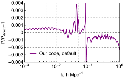
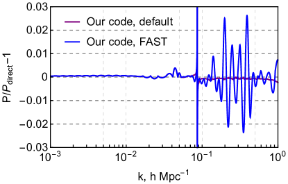
Figure 1: Residuals between our calculation of the one-loop matter power spectrum contribution and the direct numerical evaluation for the default settings (left panel) and in the “FAST” mode (right panel).

Let us now discuss the accuracy of our code, using the one-loop real-space calculations as an example. The purpose of this comparison is to show that our FFTLog routine has comparable precision to that of direct numerical integration.

The residuals between the FFTLog-based calculation and the direct numerical evaluation of the one-loop matter power spectrum are shown in Fig. 1. The singularity at $k\approx 0.1\leavevmode\nobreak\ h/$Mpc reflects the fact that the one-loop spectrum crosses zero in this region. We show the results both for the default precision with $N_{\rm FFTLog}=256$ and for the fast mode with $N_{\rm FFTLog}=128$. The default choice of $N_{\rm FFTLog}=256$ is seen to provide a relative accuracy $\sim 0.1\%$ over the range of wavenumbers $k\lesssim 0.2\leavevmode\nobreak\ h$/Mpc, as relevant for future galaxy surveys. Note that the relative accuracy quoted here does not depend on time; the absolute accuracy actually increases at high redshifts.

However, the $0.1\%$ accuracy of the one-loop correction can be somewhat excessive in many cases. For this reason, for all practical applications the user is encouraged to run the code in the fast mode. Whilst this provides us with a somewhat lower accuracy $\sim 1\%$, there is a significant speed gain. On the one hand, this numerical error is still smaller than the two-loop contribution omitted in our model. On the other hand, the one-loop contribution itself must be a small correction to the linear power spectrum in order for perturbation theory to make sense. Thus, the $\mathcal{O}(1\%)$ accuracy on the one-loop correction translates into the $\mathcal{O}(0.1\%)$ accuracy on the total power spectrum. Therefore, the fast mode seems to be sufficient for the bulk of practical applications in which the one-loop power spectrum is used as a model. To explicitly verify this, we have rerun the MCMC analysis of the BOSS data from Ref. [13] and the analysis of the large N-body simulation data from Ref. [16]. In both cases, fast and default modes yielded indistinguishable results.

4.2 Wiggly-non-Wiggly Splitting

The algorithm for wiggly-non-wiggly splitting implemented in the code is based on the discrete spectral analysis method proposed in Ref. [86]. The main idea is to Fourier transform the power spectrum to position space, localize the BAO peak, remove it, and smoothly interpolate the correlation function in the previous location of the peak. For computational efficiency this is done by means of a discrete Fourier transform. In practice, we do the following:

1. Sample an array of $\mathop{\rm ln}\nolimits(kP_{\mathrm{lin}}(z,k))$ in $2^{16}$ points over the range $[7\cdot 10^{-5},7]\,$Mpc^-1;

2. Fast sine transform (FST) this array;

3. Interpolate the odd and even harmonics using splines;

4. Remove the harmonics spanning the range of indices $[120,240]$, see Fig. 2. These harmonics correspond to the BAO peak for the comoving sound horizon at decoupling: $r_{d}\sim 150$ Mpc; We have found that this choice of the boundaries works well for the variations of $r_{d}$ in the range $(130,170)$ Mpc;

5. Interpolate the FST harmonics in the BAO range;

6. FST back the new coefficients to recover $\mathop{\rm ln}\nolimits(kP_{\text{nw}}(k))$.

The resulting wiggly power spectrum $P_{\text{w}}\equiv P_{\mathrm{lin}}-P_{\text{nw}}$ is shown in the right panel of Fig. 2. It is important to stress that we work in units of Mpc, such that the splitting is insensitive to $h$. The only cosmology-sensitive part of our procedure is the location of the BAO peak, which corresponds to the comoving sound horizon $r_{d}$. However, $r_{d}$ is a very weak function of cosmology. For instance, in $\Lambda$CDM $r_{d}\propto\omega_{m}^{-0.25}\omega_{b}^{-0.12}$ [13]. Given this reason, we use the same frequency cuts in the wiggly-non-wiggly procedure during MCMC scans over different cosmologies. Alternatively, we have tried an algorithm which rescales the frequency cuts “on-the-fly” according to the value of $r_{d}$ which is being sampled by the code. The difference between the two procedures is negligibly small and does not affect parameter inference even from the large-volume PT challenge simulation data [16].

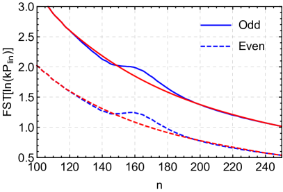
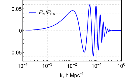
Figure 2: Left: Visualization of our wiggly-smooth splitting algorithm. We show even and odd discrete Fast Sine Transform coefficients of $\mathop{\rm ln}\nolimits(kP_{\mathrm{lin}}(k))$ for the range of indices relevant for the BAO before (in blue) and after (in red) the splitting. Right: The resulting wiggly power spectrum normalized to the smooth one.

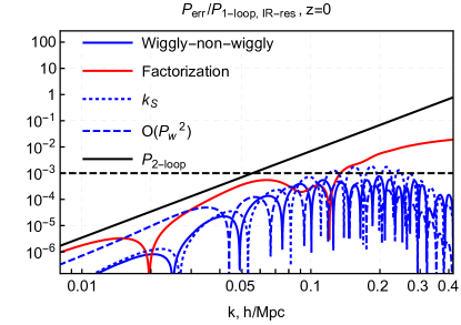
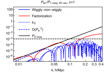
Figure 3: Errors introduced by various approximations in IR resummation relative to the two-loop contribution at $z=0$ (left panel) and $z=1$ (right panel). See the main text for detail.

4.3 Error Budget of IR Resummation

In Section 2.5 we listed various sources of error in our implementation of IR resummation. It was argued that these errors are under control, i.e. their contributions can be minimized to arbitrary small values. This is a theoretical statement, which may not hold in reality due to choices made in practical implementation. In this subsection, we will explicitly show that the residual error of the one-loop power spectrum including IR resummation is smaller than the two-loop contributions. Let us discuss each problematic ingredient separately.

Wiggly-non-Wiggly decomposition. The error introduced by our splitting procedure is always smaller than the two-loop corrections. One can argue that this is a generic statement that can be generalized to higher orders. Indeed, imagine that the BAO were described by an analytic harmonic function such that one could find an exact analytic expression for $P_{\rm nw,\,true}$. Imagine now that instead of using this analytic expression we perform a numerical wiggly-non-wiggly decomposition that introduces some intrinsic error $\Delta P_{\rm w-nw}\ll P_{\rm lin}$,

$$P_{\rm nw}=P_{\rm nw,\,true}+\Delta P_{\rm w-nw}\,,\quad P_{\rm w}=P_{\rm w,\,true}-\Delta P_{\rm w-nw}\,.$$ (4.11)

Now let us perform a leading order tree-level calculation,

$$\begin{split}P_{\rm LO}=P_{\rm nw}+{\rm e}^{-\Sigma^{2}k^{2}}P_{\rm w}=P_{\rm nw,\,true}+{\rm e}^{-\Sigma^{2}k^{2}}P_{\rm w,\,true}+\Delta P_{\rm w-nw}(1-{\rm e}^{-\Sigma^{2}k^{2}})\,.\end{split}$$ (4.12)

We see that at small wavenumbers, the wiggly-non-wiggly error cancels when we sum up the wiggly and smooth parts. The residual error term on the r.h.s. can be Taylor expanded and compared to the one-loop contribution at low $k$’s,

$$\Delta P_{\rm w-nw}(1-{\rm e}^{-\Sigma^{2}k^{2}})\approx\Sigma^{2}k^{2}\Delta P_{\rm w-nw}\ll k^{2}\sigma_{v}^{2}P_{\rm lin}\,,$$ (4.13)

where $\sigma^{2}_{v}\approx 36D^{2}(z)$ [Mpc$/h]^{2}$ is the variance of the linear displacement field, which controls the size of the one loop correction at low $k$. A similar calculation can be repeated at one-loop order. Given this observation, one can argue that as long as the wiggly-non-wiggly splitting error $\Delta P_{\rm w-nw}\ll P_{\rm lin}$ is much smaller than the power spectrum itself, the residual error of a $n$-loop calculation will be smaller than the $n+1$ loop correction. In Fig. 3 we show the residuals between the two one-loop spectra produced by changing the cuts of the Fourier harmonics. The difference generated by the wiggly-smooth procedure is clearly much smaller than the two-loop contribution and can be safely neglected.

Dependence on $k_{S}$. This ambiguity is intrinsic to the IR resummation procedure. However, it was shown in Refs. [49, 51] that the effect reduces at higher loop orders. Thus, the error due to the separation scale choice is always under rigorous perturbative control. To estimate it, we compute the residuals between the two spectra evaluated with $k_{S}=0.1\leavevmode\nobreak\ h$/Mpc and $k_{S}=0.2\leavevmode\nobreak\ h$/Mpc, and display the result in Fig. 3.

Factorization. Another source of error can be the approximate treatment of IR resummation in redshift space. Recall that, in principle, one ought to compute anisotropic 3-dimensional integrals, where the FFTLog algorithm cannot be directly applied. However, it is possible to approximately factorize the BAO damping by neglecting terms which are formally either higher order or exponentially small. For that, one should, essentially, repeat the same arguments as for the wiggly-non-wiggly decomposition, see Ref. [49, 51] for more detail.

In practice, we have checked that these terms are indeed smaller than the two-loop corrections at redshifts relevant for future surveys. In order to estimate this error we computed the difference between the full formula for the one-loop matter power spectrum (2.27) and its “factorized” version (2.32). Crucially, the residual generated by the factorization is a smooth function without a pronounced BAO feature. The reason behind this is that the factorization mostly affects the $P_{22}$-like integrals, in which the oscillating residuals are integrated over and hence washed out. The absence of features suggests that even if we neglected the theoretical error associated with two loops completely, this residual could be absorbed by the counterterms without biasing cosmological parameters in a real data analysis.

One may wonder what happens if we approximate the IR-resummation of one-loop redshift-space integrals with a direction-independent damping exponent (as it is the case in real space). Naïvely, this prescription would guarantee the absence of smooth residuals in the loop integrals. However, we have found that this approximation leads to non-negligible oscillation residuals in the density and velocity spectra, motivating the factorization prescription. These residuals are mostly produced by $P_{13}$-like integrals, for which the factorization procedure is exact and fast, thus there is no need to use the isotropic damping template. The most time-consuming process is the IR resummation of the $P_{22}$-like integrals, for which the difference between the direction-independent and full anisotropic templates was found to be quite small. Approximating the BAO damping of the $P_{22}$ integrands with the direction-independent template notably reduces the computational cost of IR resummation. This introduces $\lesssim 0.1\%$ error on the full power spectra, which is smaller than the neglected two-loop contributions on mildly-nonlinear scales. Even though this approximation seems promising, it has not yet been fully included in the current version of the code. Currently, we have implemented this method only for the $P_{22}$-like integrals of biased tracers; we plan to run more thorough tests before implementing it for the matter loop integrals as well.

We stress that we have implemented the full factorization formula with the anisotropic damping factor for the $P_{13}$-like bias integrals produced by the operator $\mathcal{F}_{\mathcal{G}_{2}}$. This formula is exact for these types of integrals.

Corrections of order $\mathcal{O}(P^{2}_{\rm w})$. Finally, we have checked that the terms $\sim P^{2}_{\text{w}}$ omitted in the IR resummation procedure of Ref. [49] are indeed negligible. In principle, these corrections can be taken into account at zeroth order at no additional cost, but their contribution is so small that they are irrelevant for all practical applications.

All the sources of error related to IR resummation are shown in Fig. 3. We see that the biggest error is introduced by the factorization procedure, but its contribution is quite smooth and its slope matches the shape of the two-loop contribution.

4.4 Evaluation of Redshift Space Multipoles

When neither IR resummation nor the AP effect are present, the code can be greatly expedited by performing the $\mu$-integrals analytically. In this case we use the explicit FFTLog matrices directly for the power spectrum multipoles. This calculation is initiated if the flag “IR resummation = No” is passed to the code. Note the AP effect is not implemented in this case. If the flag “IR resummation = Yes” is passed instead, a different routine is performed; we separately compute all Fourier integrals that multiply different powers of $\mu^{2}$ (see Eq. (4.8)) and use the following algorithm:

1. Compute each loop integral separately for wiggly and non-wiggly components; First, we evaluate it for the non-wiggly input power spectra only. Second, we compute the one-loop integrals with one entry of $P_{\rm w}$ and one entry of $P_{\rm nw}$;

2. Suppress the wiggly one-loop spectra with the anisotropic damping factor;

3. Combine these terms and add the tree-level IR-resummed part. This allows us to arrive at the final expression for $P_{\rm gg}(z,k,\mu)$ given in Eq. (2.32);

4. Map the arguments $(k,\,\mu)\to(k_{\rm obs},\,\mu_{\rm obs})$ as dictated by the AP conversion for an input cosmological model;

5. Perform the angular integrals over $\mu_{\rm obs}$ from Eq. (2.36) using the pre-computed Gaussian quadrature with 40 weights.

Note that there is only one numerical routine that performs the Legendre integrals over $\mu$ both for IR-resummation and the AP distortions. If one needs to take into account the AP-distortions but not IR resummation, one can setthe BAO damping factor, $\Sigma_{\rm tot}$, to zero. Moreover, the AP effect can be computed only if all three flags “RSD = Yes”, “IR resummation = Yes”, and “AP = Yes” are passed to the code. If necessary, one could compute the multipoles induced by the AP effect in real space by setting the growth factor $f=0$ before the RSD module is executed.

4.5 Neutrino Masses

Massive neutrinos require some special treatment. Strictly speaking, our method is not applicable if the growth rate is scale-dependent. In this case, one cannot use the usual EdS perturbation theory kernels, and the full calculation of time-and-scale dependent Green’s functions is needed [87, 88]. However, these references showed that for dark matter in real space, the difference between the full calculation and the EdS approximation is very small for realistic neutrino masses. This suggests that it is safe to use our EdS-based FFTLog calculations in this case.

To approximately incorporate massive neutrinos in the calculation of biased tracers, we use the linear power spectrum for the “cold dark matter+baryons” (“cb”) fluid as an input in all loop calculations. This prescription has been advocated on the basis of N-body simulations in [89, 90, 91, 90, 92, 93]; besides, Refs. [94, 95] claimed its importance for the neutrino mass measurement. The “cb” power spectrum is a default input of our non-linear module. If necessary, one can use the total matter density via the flag “cb=No.”

The situation is more complicated in redshift space. Just like in the biased tracer case, N-body simulations (e.g. [93]) suggest that one has to use the linear logarithmic growth factor $f_{\rm cb}$ of the “cb” fluid. Then the halo power spectra of N-body simulations approach the Kaiser prediction [74] evaluated with the “cb” quantities. Crucially, for observationally allowed neutrino masses, the scale-dependence of $f_{\rm cb}$ is around $0.1\%$ on large scales where the definition of $f_{\rm cb}$ is meaningful. Strictly speaking, the presence of this scale-dependence invalidates our whole redshift-space one-loop calculation including IR resummation and calls for a computation of the appropriate Green’s functions. However, given that this effect is very small, we will neglect it and use the EdS approximation with a scale-independent approximation for $f_{\rm cb}$. In principle, one can include the effect of appropriate Green’s functions by perturbatively expanding around the EdS kernels. We leave this for future work.

Overall, in the presence of massive neutrinos, we use the same FFTLog-EdS formulas as before, but apply them to the linear “cb” power spectrum, including the suppression at short-scales by massive neutrinos’ free-streaming. At any required redshift, the code takes the power spectrum at this exact time, such that the linear time-dependence of the neutrino suppression is taken into account. This approach is justified by N-body simulations of Ref. [93], which showed that the leading effect of massive neutrinos is always a suppression of the linear power spectrum, and any residual scale-dependence of this suppression is insignificant even for volumes as large as $100$ (Gpc/$h)^{3}$. This observation was also confirmed in various forecasts, e.g. [96, 17]. Given these reasons, we expect that using the usual FFTLog formulas in the presence of massive neutrinos will be a good approximation even for future surveys like DESI or Euclid.

4.6 Non-Standard Extensions of $\Lambda$CDM

The code in its current form can be used without any limitations for all non-minimal cosmological models that do not require modification of the perturbation theory kernels. One such example is the Early Dark Energy (EDE) model, in which the standard $\Lambda$CDM early universe physics is significantly modified in an attempt to resolve the Hubble tension [97]. CLASS-PT has been already successfully used to put the strongest constraints to date on the EDE model from the combination of the CMB and LSS data [98] (see also [99]).

In principle, CLASS-PT can be extended even to those cases which require modifications in the mode-coupling kernels, e.g. modified gravity. If these models do not violate the Equivalence Principle, one has to simply recompute the perturbation theory matrices incorporating the new kernels from these extended models. In this case, the body of the code does not need to be modified. If the Equivalence Principle is violated, IR resummation must be altered accordingly, see Refs. [100, 101].

4.7 Modified CMB Lensing Routine

In certain situations, it may be useful to have some alternative estimate for non-linear corrections that can be used instead of HALOFIT for the CMB lensing calculations. This is clearly the case for exploration of the non-standard cosmological models for which the HALOFIT fitting formula was not calibrated. Since the non-linear corrections relevant for CMB lensing are relatively small for angular multipoles $\ell<\text{few}\times 10^{3}$ [102], one may expect that perturbation theory gives reasonably accurate results for current lensing data such as, e.g. the Planck measurements. One technical difficulty in applying perturbation theory to CMB lensing is the significant width of the lensing kernel. This requires non-linear corrections from many different redshifts, whose full calculation is very time-consuming. However, given that the perturbations of the lensing potential are only very mildly-nonlinear, and given the statistical errors of current lensing data, the accuracy of non-linear corrections around $\sim 1\%$ is tolerable. In this case one can adopt the following simple approximation scheme:

1. Compute the full matter power spectrum $P^{\rm ref}_{\rm 1-loop}$ at some fixed reference redshift $z_{\rm ref}$;

2. Obtain the spectra at different redshifts $z_{i}$ by rescaling $P^{\rm ref}_{\rm 1-loop}$ with scale-independent linear growth factors,

   $$P_{\rm 1-loop}(z_{i},k)=\left(\frac{D(z_{i})}{D(z_{\rm ref})}\right)^{4}P^{\rm ref}_{\rm 1-loop}(z_{\rm ref},k)\,.$$

This procedure is exact in EdS if we neglect the time-dependence of IR-resummation and counterterms. The effect of both is around $1\%$ on mildly non-linear scales and hence can be neglected for our purposes.

Our modified lensing module was tested on the Planck 2018 data in Ref. [14], where it was found to give the same result as HALOFIT for $\nu\Lambda$CDM and $\nu\Lambda$CDM+$N_{\rm eff}$ models. However, we would like to stress that its accuracy has not been extensively tested for the precision required for future experiments.

5 Results and Performance

In this Section we show some results and discuss the performance of our code. All plots are generated with the Jupyter notebook that can be downloaded from the GitHub page of the code. Our timing results were obtained on a MacBook Pro Retina Early 2015 laptop, with a 2.7 GHz Intel Core i5 processor and using OS X version 10.11.6. In all cases, CLASS was run with the C compiler gcc-6.1.0. Our classy is based on Python 2.7.10, numpy 1.14.5, and scipy 0.19.0. The results of this Section will be presented for the non-linear power spectrum using the We use the following nuisance parameters:

$$\begin{split}&c_{s}^{2}=1\leavevmode\nobreak\ [\text{Mpc}/h]^{2}\,,\quad R_{*}^{2}=c_{0}=5\leavevmode\nobreak\ [\text{Mpc}/h]^{2}\,,\quad P_{\rm shot}=5\times 10^{3}\leavevmode\nobreak\ [\text{Mpc}/h]^{3}\,,\\ &b_{1}=2\,,\quad b_{2}=-1\,,\quad b_{{\cal G}_{2}}=0.1\,,\quad b_{\Gamma_{3}}=-0.1\,,\\ &c_{2}=15\leavevmode\nobreak\ [\text{Mpc}/h]^{2}\,,\quad c_{4}=-5\leavevmode\nobreak\ [\text{Mpc}/h]^{2}\,,\quad\tilde{c}_{\nabla^{4}_{\bf z}\delta}=100\leavevmode\nobreak\ [\text{Mpc}/h]^{4}\,.\end{split}$$ (5.1)

These are consistent with the values extracted from high-resolution BOSS mock galaxy catalogs and the actual BOSS survey data [13]. We stress that these nuisance parameters should be fitted from the data in any realistic analysis.

5.1 Examples of Nonlinear Spectra

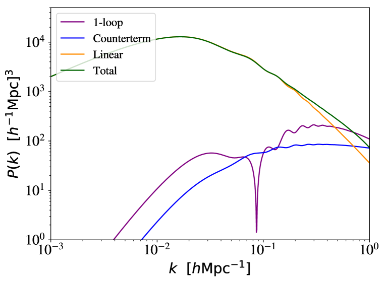
Figure 4: Breakdown of different contributions to the one-loop matter power spectrum of dark matter in real space.

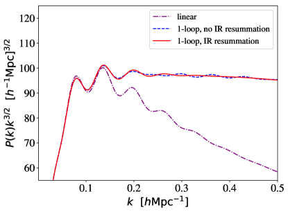
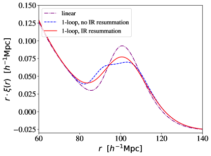
Figure 5: Left panel: The total power spectrum with and without IR resummation, along with the linear theory prediction. All spectra are multiplied by $k^{3/2}$ for better visualization. Right panel: The position space correlation functions extracted from the same calculations.

Fig. 4 shows the breakdown of different contributions to the matter power spectrum in redshift space without IR resummation. In Fig. 5 we show the effect of IR resummation. Without this procedure, the one-loop correction fails to capture the shape of the BAO wiggles and even their frequency. This result is well known in the literature [46, 49] and it explicitly shows that IR resummation is a necessary ingredient of any realistic non-linear calculation. For comparison, we also display the linear theory power spectrum.

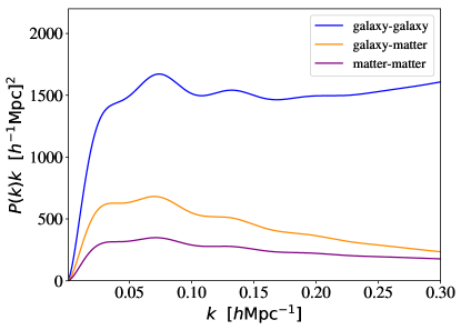
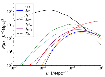
Figure 6: Left panel: One loop predictions for the matter-matter, matter-galaxy and galaxy-galaxy power spectra of the BOSS-like galaxy sample. Right panel: breakdown of different bias contributions to the one-loop galaxy power spectrum.

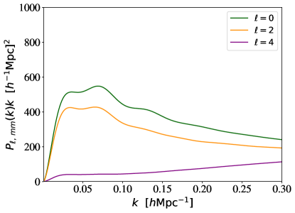
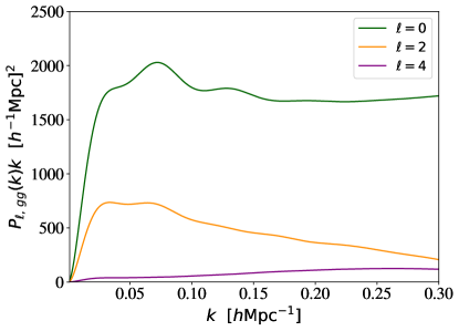
Figure 7: Left panel: Redshift-space multipoles of the matter power spectrum. Right panel: the same for the galaxy power spectrum of the BOSS-like sample.

In Fig. 6 we show the galaxy-galaxy, galaxy-matter and matter-matter spectra in real space (left panel) and the breakdown of different bias loop corrections (right panel). Fig. 7 displays redshift-space multipoles of dark matter (left panel) and BOSS galaxies (right panel). Note that in the latter case we have included the $\tilde{c}_{\nabla^{4}_{\bf z}\delta}$-counterterm.

Fig. 8 shows the lensed temperature (TT) and the CMB lensing potential power spectra computed in perturbation theory and with HALOFIT (divided by the linear theory prediction), as well as the relative difference between the two. One sees that the difference between the PT and HALOFIT predictions is less than $0.1\%$ for the lensed TT spectrum and around $\sim 2\%$ at the small-scale part of the $C_{\ell}^{(\phi\phi)}$ spectrum. These differences can be taken as an estimate for the theoretical error associated with the modeling of non-linear corrections. We believe that the residual between the PT and HALOFIT spectra can be reduced by an appropriate tuning of the dark matter effective sound speed $c_{s}^{2}$. Moreover, a better description can be wrought by combining the two methods; perturbation theory is very accurate on mildly non-linear scale, whereas the N-body based fitting formulas capture the leading behavior in the fully non-linear regime. The exploration of the matter power spectrum on these short scales can be done with relatively cheap small-box simulations. A thorough study of this possibility is left for future work.

Run	Real space	IR resum.	RSD	IR+RSD	IR+RSD+AP
Default mode
Matter	0.036 (0.036)	0.175 (0.036)	0.375 (0.375)	0.75 (0.62)	0.76 (0.63)
Tracers	0.21 (0.21)	0.35 (0.21)	0.89 (0.89)	1.27 (1.12)	1.30 (1.14)
FAST mode
Matter	$6.3\leavevmode\nobreak\ (6.1)\times 10^{-3}$	0.14 (0.0061)	0.063 (0.061)	0.22 (0.09)	0.22 (0.09)
Tracers	0.033 (0.034)	0.17 (0.034)	0.14 (0.14)	0.31 (0.18)	0.31 (0.18)

Table 1: Performance of the code for baseline precision runs. We show the execution time in [sec.] as follows: $t_{\rm full}(t_{\rm FFTLog})$, where $t_{\rm full}$ is the full end-to-end time taken by the non-linear module, and $t_{\rm FFTLog}$ is the time elapsed during the matrix multiplication with FFTLog.

5.2 Performance

Let us discuss now the performance of our numerical routine. Table 1 displays the run time for various spectra computed by CLASS-PT in the default (high-precision) and fast modes. These values are the typical ones obtained on authors’ laptops; some variation is expected for different machines. Importantly, the execution time reduces roughly by a factor of 4 in the fast mode, which uses a grid twice smaller than the default one. This is a consequence of the fact that the most time-consuming process is matrix multiplication, which very roughly scales as $N_{\rm FFTLog}^{2}$.

We see that basic runs for the real-space power spectrum without IR resummation are quite fast. Their speed is comparable to that of other methods, e.g. FAST-PT [22]. IR resummation and bias tracers increase the execution time by a factor of $\sim 5$ separately. Since these two procedures are independent, this results in an overall speed loss by a factor of $10$ compared to the basic run. Redshift space distortions affect the calculation in two ways. First, there are additional convolution integrals that appear in multipole moments. Second, redshift space requires a more sophisticated IR resummation procedure, which again increases the number of convolution integrals even further. When the two effects are combined, the execution time reaches the level of 1.3 second for high precision settings and 0.3 seconds in the fast mode. The inclusion of the AP effect does not notably affect the speed.

5.3 Cautionary Remarks

There are several caveats to be borne in mind when using our code.

First, at face value, the code can be used for any beyond-$\Lambda$CDM cosmology provided that the structure of the perturbation theory kernels is not modified. This is the case for the bulk of extended models explored by Planck [1]. However, the numerical implementation choices made in the code have not been extensively tested for cosmological models that are extremely different from the Planck best-fitting cosmology. Some of our choices, i.e. the frequency cuts in the wiggly-non-wiggly decomposition, would have to be reconsidered if someone wants to explore, say a model with a large numbers of neutrino species, e.g. $N_{\rm eff}=42$.

Second, many implementation choices in our code were made to maximize precision on large scales $k\leq 1\leavevmode\nobreak\ h$/Mpc. Our baseline realization of the non-linear calculation must not be used for $k\gtrsim 3\leavevmode\nobreak\ h$/Mpc. Therefore, our code is not suitable for small-scale galaxy clustering or some lensing calculations where a significant amount of signal comes from the highly nonlinear scales. One also must carefully choose $k_{\rm max}$ as a function of redshift, recalling that the loop corrections reduce at high-$z$, allowing smaller scales to be probed. The maximal wavenumber to which our code can be used to extract information from the matter clustering corresponds to the scale where the loop expansion blows up, i.e. whence the two-loop correction becomes comparable to the tree-level prediction. Using the fit to the two-loop power spectrum from Refs. [38, 17], this scale can be estimated as

$$k_{\rm NL}(z)=0.45[D(z)]^{-\frac{4}{3.3}}\leavevmode\nobreak\ h\text{Mpc}^{-1}\,.$$ (5.2)

The use of non-linear corrections computed with our code is, strictly speaking, justified only for $k<k_{\rm NL}$. The corresponding validity domain is shown in Fig. 9 as a function of redshift.

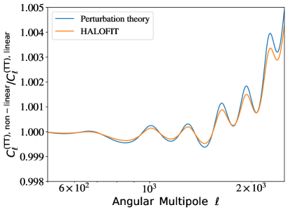
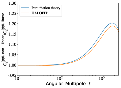
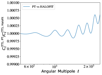
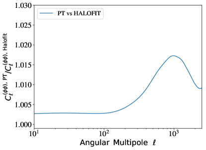
Figure 8: Upper left panel: The lensed TT CMB power spectrum computed with perturbation theory (PT) and HALOFT, normalized to the linear theory prediction. Upper right panel: A similar fraction for the CMB lensing potential power spectrum. Lower panels:Ratio of the non-linear models for the lensing potential power spectrum and the lensed CMB TT power spectrum.

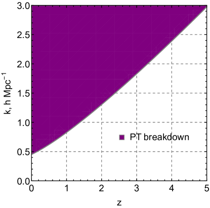
Figure 9: Regime of applicability of the one-loop corrections coputed by our code.

One obvious caveat is that our code does not include relativistic corrections and wide-angle effects, and therefore it should be used with care on very large scales. Furthermore, it does not have corrections to the linear bias due to local primordial non-Gaussianities. All of these corrections do not require nonlinear calculations and can be easily added if necessary.

6 Application to the BOSS Data

In this Section, we illustrate an application of our code to the analysis of the final BOSS data release [7]. To this end, we interface CLASS-PT with the MCMC sampler montepython v3.0 [12, 6]. We will analyze a full-shape likelihood built out of the publicly available BOSS data and products taken from, see Refs. [103, 104] for more detail. This likelihood has already been used in Refs. [13, 14, 15], where one can find all technical details. We repeat it here just as an illustration.

As an aside, we would like to mention that the shape of the galaxy power spectrum has been used for cosmological parameter measurements since the dawn of galaxy surveys, see e.g. [105, 106, 107, 108, 109, 110]. This practice, however, has been abandoned in the recent full-shape analyses that are based on the methodology borrowed from the BAO measurements [111, 7, 104]. These analyses infer distance information by studying how the AP effect distorts some fixed-shape power spectrum template. The fixed template method is also adopted in the measurement of rms velocity fluctuation $f\sigma_{8}$. This method has a number of limitations which can compromise the cosmological analysis of future high-precision data [17, 13].

An alternative to the fixed shape approach is to return to the methodology of measuring the cosmological parameters of a given model from the full power spectrum. This is the standard method adopted in the analyses of the CMB data [1]. An important advantage of this method is its universality: it can be applied to any model including beyond $\Lambda$CDM cosmologies. In this Section, for illustration purposes, we present the constraints obtained in this way for the base $\Lambda$CDM model. It is straightforward to repeat this analysis for more complicated beyond-$\Lambda$CDM models, see e.g. [25] for the analysis within $w$CDM and [14, 15] for $\nu\Lambda$CDM and $\nu\Lambda$CDM+$N_{\rm eff}$. We stress that the key novelty of our analysis is the most advanced theoretical model for the nonlinear power spectrum. In other aspects our method closely follows the ones proposed and used decades ago.

Our likelihood covers the pre-reconstructed redshift-space power spectra of BOSS galaxies across two non-overlapping redshift bins, $0.2<z<0.5$ and $0.5<z<0.75$ from two patches of the sky (North Galactic Cap and South Galactic Cap, NGC and SGC). We use the momentum range $[0.01,0.25]\leavevmode\nobreak\ h/$Mpc, which is stable w.r.t. instrumental systematics and two-loop corrections, that are omitted in our theory model. We fit the BOSS galaxy power spectra assuming the base flat $\Lambda$CDM model, fixing the tilt of the primordial power spectrum of scalar fluctuations $n_{s}$ and the physical baryon density $\omega_{b}$ to the Planck 2018 best-fit values [1];

$$n_{s}=0.9649\,,\quad\omega_{b}=0.02237\,.$$ (6.1)

In principle, we can also scan over these parameters in our chains, see e.g. [13, 15], but do not do it here for simplicity. The role of the priors (6.1) and their impact on parameter inference have been thoroughly investigated in Ref. [13]. Following Ref. [1], we approximate the neutrino sector with only one massive eigenstate and fix its mass to the lowest value allowed by the oscillation experiments, $m_{\nu}=0.06$ eV. This choice is made purely for demonstration purposes. We believe that it is more appropriate to scan over this unknown parameter, as is done in Refs. [13, 14, 15].

Our MCMC chains sample the remaining cosmological parameters of the minimal $\Lambda$CDM model: the physical density of dark matter $\omega_{cdm}$; the Hubble constant $H_{0}$; the amplitude of primordial scalar fluctuations $A_{\rm s}$. We do not assume any priors on these parameters. To be more precise, we scan over $A^{1/2}_{s}$ normalized to the Planck best-fit value,

$$A^{1/2}=\text{norm}\equiv\left(\frac{A_{\rm s}}{A_{\rm s,\,Planck}}\right)^{1/2}\,.$$ (6.2)

This choice allows us to treat $A_{s}$ as a nuisance parameters and quickly scan over it, which leads to better convergence. We have run our analysis both in the fast and default modes and obtained identical results.

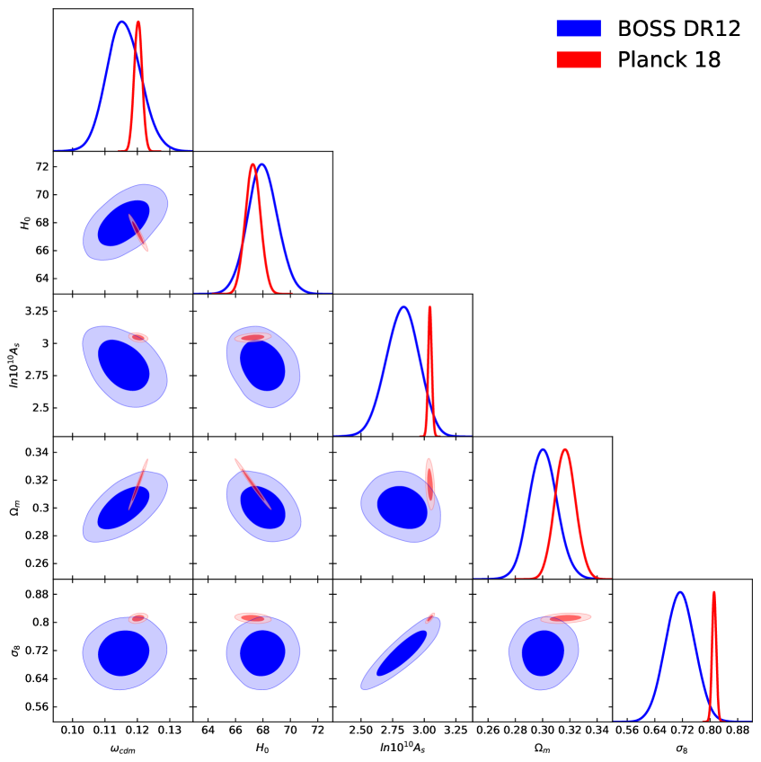
Figure 10: The posterior distribution for $\omega_{cdm},\leavevmode\nobreak\ H_{0},\leavevmode\nobreak\ \mathop{\rm ln}\nolimits(10^{10}A_{s})$ and derived parameters $\Omega_{m},\leavevmode\nobreak\ \sigma_{8}$ inferred from the joint BOSS DR12 full-shape likelihood. For comparison we also show the Planck 2018 posterior (red contours) for the same model (base flat $\Lambda$CDM). $H_{0}$ is quoted in units [km/s/Mpc].

BOSS DR12	best-fit	mean $\pm 1\sigma$
$\omega_{cdm}$	$0.1169$	$0.1159_{-0.0054}^{+0.0050}$
$H_{0}$	$67.91$	$67.98_{-1.1}^{+1.1}$
$\mathop{\rm ln}\nolimits(10^{10}A_{s})$	$2.83$	$2.82^{+0.13}_{-0.13}$
$\Omega_{m}$	$0.3034$	$0.3006_{-0.010}^{+0.010}$
$\sigma_{8}$	$0.716$	$0.710^{+0.043}_{-0.043}$

Planck 2018	best-fit	mean $\pm 1\sigma$
$\omega_{cdm}$	$0.1204$	$0.1202_{-0.0012}^{+0.0012}$
$H_{0}$	$67.29$	$67.28_{-0.55}^{+0.53}$
$\mathop{\rm ln}\nolimits(10^{10}A_{s})$	$3.04$	$3.045_{-0.015}^{+0.014}$
$\Omega_{m}$	$0.3168$	$0.3166^{+0.0075}_{-0.0075}$
$\sigma_{8}$	$0.8099$	$0.8117_{-0.006}^{+0.0057}$

Table 2: The results of our MCMC analysis for the joint BOSS DR12 full-shape likelihood (left panel). For comparison we also show the results from the final Planck data release [1] (right table) for the same cosmological model used in our analysis (base $\Lambda$CDM with a fixed neutrino mass). $H_{0}$ is quoted in [km/s/Mpc] units.

As far as the nuisance parameters are concerned, we fit them for each galaxy sample separately, due to different calibration and selection functions. We have seven nuisance parameters in total (sampling all in the “fast” mode from Ref. [114] alongside $A^{1/2}$ ): linear bias $b_{1}$, quadratic bias $b_{2}$, tidal bias $b_{{\cal G}_{2}}$, shot noise $P_{\rm shot}$ and three counterterms $c_{0},c_{2},\tilde{c}$. The cubic bias $b_{\Gamma_{3}}$ is set to zero. The detailed description of these parameters can be found in Ref. [13]. We chose the following priors for the bias parameters:

$$\begin{split}&b_{1}A^{1/2}\in(1,4)\,,\quad b_{2}A^{1/2}\sim\mathcal{N}(0,1)\,,\\ &b_{\mathcal{G}_{2}}A^{1/2}\sim\mathcal{N}(0,1)\,,\quad P_{\rm shot}\times[h^{-1}\text{Mpc}]^{-3}\sim\mathcal{N}(5000,5000^{2})\,,\\ \end{split}$$ (6.4)

and the counterterms:

$$\begin{split}&c_{0},c_{2}\times[h^{-1}\text{Mpc}]^{-2}\sim\mathcal{N}(0,30^{2})\,,\quad\tilde{c}\times[h^{-1}\text{Mpc}]^{-4}\sim\mathcal{N}(500,500^{2})\,,\\ \end{split}$$ (6.5)

which are selected such that the corresponding shapes do not exceed the linear theory spectra on the scales used for the fit. Furthermore, the priors for the bias parameters are motivated by the coevolution model and results of N-body simulations. Alternatively, one could fix the priors on the nuisance parameters using the method proposed in Ref. [16]. We discuss the treatment of nuisance parameters, including their priors and measurements, in Appendix C. All in all, the priors for nuisance parameters do not significantly affect the constraints on cosmological parameters.

The results of our analysis are shown in Fig. 10 and in Table 2, where we separated the directly sampled parameters $(\omega_{cdm},H_{0},A_{s})$ from the derived ones $(\Omega_{m},\sigma_{8})$. These constraints agree well with those reported in Ref. [13], although the priors used in our present analysis are slightly different. Note that presented BOSS constraints should always be taken in conjunction with the priors on $\omega_{b},n_{s}$ and $m_{\nu}$ made in our analysis. For comparison, we also show the results of our analysis of the baseline Planck 2018 likelihood [116] for the same cosmological model.

We publicly release our BOSS Montepython likelihoods in a separate repository https://github.com/Michalychforever/lss_montepython. The likelihoods are available is the standard and optimized versions. The latter includes the Fourier-space window function treatment and analytic marginalization over the nuisance parameters $\{c_{0},c_{2},\tilde{c},P_{\rm shot}\}$ along the lines of Ref. [75].

7 Conclusions

In this paper we have presented a new open-source extension of the Boltzmann solver CLASS that incorporates one-loop perturbation theory calculations. This module, called CLASS-PT, computes Fourier-space power spectra of matter and biased tracers in real and redshift space. It contains all ingredients required for the application to data: IR resummation to describe the non-linear evolution of the BAO wiggles; non-linear bias prescriptions; UV counterterms that capture the effects of poorly known short-scale physics on large scales, such as fingers-of-God and baryonic feedback. We stress that the main advantage of perturbation theory over other approaches is that it guarantees high precision on wavenumbers smaller than the nonlinear scale  $k_{\rm NL}\sim 0.5\leavevmode\nobreak\ h$/Mpc at $z=0$. Many complicated phenomena that operate on short scales drastically simplify in the long-wavelength limit, where they can be consistently and accurately taken into account.

The current execution time of CLASS-PT is fast enough to make the Markov Chain Monte Carlo analysis of redshift-space clustering data feasible. The code was already used for these purposes in References [17, 13, 14, 15, 16].

The realization of nonlinear perturbation theory as a module directly inside the Boltzmann code CLASS has many advantages. It is clearly structured, easy to modify, and designed to avoid hard-coding. Moreover, it can be readily interfaced with other software, e.g. conventional MCMC samplers such as Montepython [12, 6] and cobaya. The CLASS code is one of the standard tools established in cosmology. By writing our module directly as part of CLASS, it was our aim to make the nonlinear cosmological perturbation theory calculations more available to the broad community: now, all users familiar with CLASS can easily perform these calculations.

Like many things, CLASS-PT is ever-evolving. The first avenue of improvement is devoted to the improvement of efficiency and accuracy of our calculation. We believe that some implementation choices used in the current version of CLASS-PT may not be not optimal and will certainly be revisited in the future.

The second line of research is aimed at incorporating new non-linear effects. In particular, the FFTLog algorithm is convenient for the implementation of two-loop power spectrum and one-loop bispectrum calculations [24]. Moreover, we plan to implement the observer-dependent convolution integrals describing selection effects such as intrinsic alignment of galaxies (see Ref. [117] and references therein). Additionally, it is important to accurately take into account corrections due to the scale-dependent growth introduced, e.g. by massive neutrinos. We leave these research directions for future work.

Appendix A Redshift-Space FFTLog Master Integrals

In this Appendix we present explicit expressions for the functions appearing in the integrals (4.5). The coefficients of the integrals with one and two insertions of loop momenta read

$$\begin{split}&A_{1}(\nu_{1},\nu_{2})=\frac{1}{2}({\sf I}(\nu_{1}-1,\nu_{2})-{\sf I}(\nu_{1},\nu_{2}-1)+{\sf I}(\nu_{1},\nu_{2}))\,,\\ &A_{2}(\nu_{1},\nu_{2})=-\frac{1}{8}\Big{(}{\sf I}(\nu_{1},\nu_{2})+{\sf I}(\nu_{1},\nu_{2}-2)+{\sf I}(\nu_{1}-2,\nu_{2})\\ &\leavevmode\nobreak\ \leavevmode\nobreak\ \leavevmode\nobreak\ \leavevmode\nobreak\ \leavevmode\nobreak\ \leavevmode\nobreak\ \leavevmode\nobreak\ \leavevmode\nobreak\ \leavevmode\nobreak\ \leavevmode\nobreak\ -2{\sf I}(\nu_{1},\nu_{2}-1)-2{\sf I}(\nu_{1}-1,\nu_{2})-2{\sf I}(\nu_{1}-1,\nu_{2}-1)\Big{)}\,,\\ &B_{2}(\nu_{1},\nu_{2})=3\Big{(}{\sf I}(\nu_{1},\nu_{2})+{\sf I}(\nu_{1},\nu_{2}-2)+{\sf I}(\nu_{1}-2,\nu_{2})+\frac{2}{3}{\sf I}(\nu_{1},\nu_{2}-1)\\ &\leavevmode\nobreak\ \leavevmode\nobreak\ \leavevmode\nobreak\ \leavevmode\nobreak\ \leavevmode\nobreak\ \leavevmode\nobreak\ \leavevmode\nobreak\ \leavevmode\nobreak\ \leavevmode\nobreak\ \leavevmode\nobreak\ -2{\sf I}(\nu_{1}-1,\nu_{2})-2{\sf I}(\nu_{1}-1,\nu_{2}-1)\Big{)}\,.\\ \end{split}$$ (A.1)

For the integrals with three insertions one finds

$$\begin{split}&A_{3}(\nu_{1},\nu_{2})=-\frac{3}{16}\Big{(}{\sf I}(\nu_{1},\nu_{2})+{\sf I}(\nu_{1}-3,\nu_{2})-3{\sf I}(\nu_{1}-2,\nu_{2}-1)-{\sf I}(\nu_{1}-2,\nu_{2})+3{\sf I}(\nu_{1}-1,\nu_{2}-2)\\ &-2{\sf I}(\nu_{1}-1,\nu_{2}-1)-{\sf I}(\nu_{1}-1,\nu_{2})-{\sf I}(\nu_{1},\nu_{2}-3)+3{\sf I}(\nu_{1},\nu_{2}-2)-3{\sf I}(\nu_{1},\nu_{2}-1)\Big{)}\,,\\ &B_{3}(\nu_{1},\nu_{2})=\frac{1}{16}\Big{(}5{\sf I}(\nu_{1}-3,\nu_{2})-15{\sf I}(\nu_{1}-2,\nu_{2}-1)+3{\sf I}(\nu_{1}-2,\nu_{2})+15{\sf I}(\nu_{1}-1,\nu_{2}-2)\\ &-18{\sf I}(\nu_{1}-1,\nu_{2}-1)+3{\sf I}(\nu_{1}-1,\nu_{2})-5{\sf I}(\nu_{1},\nu_{2}-3)+15{\sf I}(\nu_{1},\nu_{2}-2)\\ &-15{\sf I}(\nu_{1},\nu_{2}-1)+5{\sf I}(\nu_{1},\nu_{2})\Big{)}\,.\end{split}$$ (A.2)

Finally, the integrals with four insertions of the loop momentum yield

$$\begin{split}&A_{4}(\nu_{1},\nu_{2})=\frac{3}{128}\Big{(}{\sf I}(\nu_{1}-4,\nu_{2})-4{\sf I}(\nu_{1}-3,\nu_{2}-1)-4{\sf I}(\nu_{1}-3,\nu_{2})+6{\sf I}(\nu_{1}-2,\nu_{2}-2)\\ &+4{\sf I}(\nu_{1}-2,\nu_{2}-1)+6{\sf I}(\nu_{1}-2,\nu_{2})-4{\sf I}(\nu_{1}-1,\nu_{2}-3)+4{\sf I}(\nu_{1}-1,\nu_{2}-2)\\ &+4{\sf I}(\nu_{1}-1,\nu_{2}-1)-4{\sf I}(\nu_{1}-1,\nu_{2})+{\sf I}(\nu_{1},\nu_{2}-4)-4{\sf I}(\nu_{1},\nu_{2}-3)\\ &+6{\sf I}(\nu_{1},\nu_{2}-2)-4{\sf I}(\nu_{1},\nu_{2}-1)+{\sf I}(\nu_{1},\nu_{2})\Big{)}\,,\end{split}$$ (A.3)

$$\begin{split}&B_{4}(\nu_{1},\nu_{2})=-\frac{3}{64}\Big{(}5{\sf I}(\nu_{1}-4,\nu_{2})-20{\sf I}(\nu_{1}-3,\nu_{2}-1)-4{\sf I}(\nu_{1}-3,\nu_{2})\\ &+30{\sf I}(\nu_{1}-2,\nu_{2}-2)-12{\sf I}(\nu_{1}-2,\nu_{2}-1)-2{\sf I}(\nu_{1}-2,\nu_{2})-20{\sf I}(\nu_{1}-1,\nu_{2}-3)\\ &+36{\sf I}(\nu_{1}-1,\nu_{2}-2)-12{\sf I}(\nu_{1}-1,\nu_{2}-1)-4{\sf I}(\nu_{1}-1,\nu_{2})+5{\sf I}(\nu_{1},\nu_{2}-4)-20{\sf I}(\nu_{1},\nu_{2}-3)\\ &+30{\sf I}(\nu_{1},\nu_{2}-2)-20{\sf I}(\nu_{1},\nu_{2}-1)+5{\sf I}(\nu_{1},\nu_{2})\Big{)}\,,\end{split}$$ (A.4)

$$\begin{split}&C_{4}(\nu_{1},\nu_{2})=\frac{1}{128}\Big{(}35{\sf I}(\nu_{1}-4,\nu_{2})-140{\sf I}(\nu_{1}-3,\nu_{2}-1)+20{\sf I}(\nu_{1}-3,\nu_{2})+210{\sf I}(\nu_{1}-2,\nu_{2}-2)\\ &-180{\sf I}(\nu_{1}-2,\nu_{2}-1)+18{\sf I}(\nu_{1}-2,\nu_{2})-140{\sf I}(\nu_{1}-1,\nu_{2}-3)+300{\sf I}(\nu_{1}-1,\nu_{2}-2)\\ &-180{\sf I}(\nu_{1}-1,\nu_{2}-1)+20{\sf I}(\nu_{1}-1,\nu_{2})+35{\sf I}(\nu_{1},\nu_{2}-4)-140{\sf I}(\nu_{1},\nu_{2}-3)\\ &+210{\sf I}(\nu_{1},\nu_{2}-2)-140{\sf I}(\nu_{1},\nu_{2}-1)+35{\sf I}(\nu_{1},\nu_{2})\Big{)}\,.\end{split}$$ (A.5)

Appendix B Brief Installation Manual

CLASS-PT is compatible with both python v2 and v3. It is installed and configured in 8 easy steps:

1. Download the OpenBLAS library from http://www.openblas.net/

2. Extract the library in a folder and configure the package by executing

   $$\$\leavevmode\nobreak\ \texttt{gmake CC=gcc FC=gfortran}$$

   in that folder.

3. Install the package via

   $$\$\leavevmode\nobreak\ \texttt{make install PREFIX=path/to/OpenBLAS}$$

4. Download and unpack CLASS-PT.

5. Change the path to OpenBLAS in CLASS-PT/Makefile to your actual path to the compiled library path/to/OpenBLAS/lib/libopenblas.a

6. Update the paths to path/to/OpenBLAS/lib/libopenblas.a in the extra_link_args of CLASS-PT/python/setup.py

7. Compile CLASS-PT as usual by typing

   $$\begin{split}&\$\leavevmode\nobreak\ \texttt{make clean}\\ &\$\leavevmode\nobreak\ \texttt{make}\end{split}$$

8. Reap the rewards of lightning-fast perturbation theory with CLASS-PT and classy!

Appendix C Treatment of nuisance parameters

Let us first discuss our choice of priors for the nuisance parameters. We assume a flat non-informative prior on $b_{1}A^{1/2}\in(1,4)$. Since the satellite fraction of the BOSS galaxy sample is quite small, most of the galaxies are centrals and hence should trace the properties of the host dark matter halos. The measurements of $b_{2}$ and $b_{{\cal G}_{2}}$ from N-body simulations [118] yield

$$b_{2}\approx-0.6\,,\quad b_{{\cal G}_{2}}\approx-0.3\quad\text{for}\quad b_{1}\approx 2\,.$$ (C.1)

Note that the values for $b_{{\cal G}_{2}}$ are also consistent with the predictions of the coevolution model [58]. On general grounds, the bias parameters are expected to be $\mathcal{O}(1)$ in the EFT, which motivates the priors $b_{2}A^{1/2},b_{{\cal G}_{2}}A^{1/2}\sim\mathcal{N}(0,1)$. Note that we have inserted $A^{1/2}\approx 1$ in the definition of our sample parameters because this choice leads to somewhat better convergence of the MCMC chains.

As far as the higher-derivative counterterms $c_{0}$ and $c_{2}$ are concerned, they are, in general, also expected to be

$$c_{0},c_{2}=\mathcal{O}(1)\times k^{-2}_{\rm NL}$$ (C.2)

The non-linear scale in redshift space depends on the velocity dispersion of the BOSS galaxies, which can be quite large. Indeed, previous BOSS full-shape analyses report $\sigma_{v}\sim 5$ Mpc/$h$ [104], which is several times larger than the real-space estimate $k^{-1}_{\rm NL}\sim 2$ Mpc/$h$. It is important to stress that the quoted measurement of $\sigma_{v}$ from Ref. [104] results from an application of a simplified fitting function, and the actual velocity dispersion can be different if one is using the full EFT model. Nevertheless, we adopt the following priors for the counterterms that are wide enough to accommodate a large velocity dispersion,

$$c_{0},c_{2}\sim\mathcal{N}(0,30^{2})\leavevmode\nobreak\ [\text{Mpc}/h]^{2}\,.$$ (C.3)

The prior for the next-to-leading order RSD counterterm $\tilde{c}$ is more subtle. Naïvely, this contribution has the order of the two-loop correction and hence has not been originally included in the one-loop EFT theory model [59, 72]. However, due to the strong fingers-of-God found in the BOSS galaxy sample, the coefficient $\tilde{c}$ turned out to be enhanced compared to the naive EFT estimates. Dedicated analyses of the BOSS mock catalogs and the real data [13] gave

$$\tilde{c}\sim\sigma_{v}^{4}\sim[5\leavevmode\nobreak\ \text{Mpc}/h]^{4}\sim 500\leavevmode\nobreak\ [\text{Mpc}/h]^{4}\,.$$ (C.4)

This motivates the prior $\tilde{c}\sim\mathcal{N}(500,500^{2})\leavevmode\nobreak\ [\text{Mpc}/h]^{4}$

Finally, as far as the constant shot noise contribution $P_{\rm shot}$ is concerned, its true value is expected to deviate from the Poissonian prediction $\bar{n}^{-1}$ due to exclusion effects [119] and fiber collisions [120]. The latter are not possible to predict from first principles and are difficult to model even in mock catalogs [121]. Thus, we adopted a more practical data-driven approach; first finding the best-fit values for $P_{\rm shot}$ from the data itself and then imposing a large conservative prior centered at this best-fit value. The Poissonian part $\bar{n}^{-1}$ has already been subtracted from the power spectrum estimator of our data. We found the residual shot noise contribution best-fits to be roughly

$$P_{\rm shot}\sim 5\cdot 10^{3}\leavevmode\nobreak\ [\text{Mpc}/h]^{3}\,,$$ (C.5)

for all the data chunks studied in this paper. This motivated the prior $P_{\rm shot}\sim\mathcal{N}(5,5^{2})\cdot 10^{3}\leavevmode\nobreak\ [\text{Mpc}/h]^{3}$, which is wide enough to accommodate absolute deviations from $\bar{n}^{-1}$ across all data samples, in particular, in the high-z SGC sample, whose Poissonian shot noise is quite large. Notice that the residual $P_{\rm shot}$ can, in principle, be negative. This fact is reflected in our prior.

We present the optimal values of the nuisance parameters found in our MCMC analysis in Tab. 3 and in Figs 11 (high-z NGC), 12 (high-z SGC), 13 (low-z NGC), 14 (low-z SGC). We differentiate between nuisance parameters for different BOSS data samples with the following superscripts:

(1) = high-z NGC, (2) = high-z SGC, (3) = low-z NGC, (4) = low-z SGC (C.6)

We stress that these parameters are obtained from a joint fit, i.e. the cosmological parameters are assumed to be the same across all samples. One can see that the best-fit values are in good agreement with the ones expected from the BOSS galaxy sample. The measured values of $c_{0},c_{2}$ and $\tilde{c}$ are indeed consistent with the estimate for the velocity dispersion effects (C.3), (C.4). Moreover, the best-fitting values of $b_{2}$ and $b_{\mathcal{G}_{2}}$ agree with the values found in the N-body simulations for the host halos similar to those of the BOSS sample (C.1). It would be interesting to further investigate if these values are also compatible with biases inferred from the bispectrum [122, 123].

Param	best-fit	mean$\pm\sigma$	95% lower	95% upper
$\omega_{cdm}$	$0.1169$	$0.1159_{-0.0054}^{+0.0050}$	$0.1061$	$0.1258$
$H_{0}$	$67.91$	$67.98_{-1.1}^{+1.1}$	$65.81$	$70.18$
$A^{1/2}$	$0.9499$	$0.9069_{-0.054}^{+0.058}$	$0.7931$	$1.016$
$\Omega_{m}$	$0.3034$	$0.3006_{-0.010}^{+0.010}$	$0.2812$	$0.3207$
$\sigma_{8}$	$0.716$	$0.710_{-0.043}^{+0.043}$	$0.627$	$0.794$
$b^{(1)}_{1}A^{1/2}$	$1.949$	$1.958_{-0.048}^{+0.05}$	$1.86$	$2.056$
$b^{(1)}_{2}A^{1/2}$	$-1.722$	$-1.766_{-0.79}^{+0.62}$	$-3.145$	$-0.2932$
$b^{(1)}_{{\mathcal{G}_{2}}}A^{1/2}$	$-0.02759$	$-0.04753_{-0.22}^{+0.19}$	$-0.466$	$0.3902$
$10^{-1}c^{(1)}_{{0}}$	$1.794$	$1.991_{-2.2}^{+2.3}$	$-2.438$	$6.494$
$10^{-1}c^{(1)}_{{2}}$	$2.192$	$1.949_{-1.9}^{+2.2}$	$-2.216$	$5.992$
$10^{-3}P^{(1)}_{{\rm shot}}$	$3.308$	$3.344_{-1.8}^{+1.7}$	$-0.1072$	$6.83$
$10^{-3}\tilde{c}^{(1)}$	$0.1775$	$0.1684_{-0.09}^{+0.086}$	$-0.008266$	$0.348$
$b^{(2)}_{1}A^{1/2}$	$2.015$	$2.024_{-0.06}^{+0.065}$	$1.897$	$2.148$
$b^{(2)}_{2}A^{1/2}$	$-0.5063$	$-0.7053_{-1}^{+0.83}$	$-2.475$	$1.179$
$b^{(2)}_{{\mathcal{G}_{2}}}A^{1/2}$	$0.05212$	$0.1852_{-0.24}^{+0.22}$	$-0.2893$	$0.6625$
$10^{-1}c^{(2)}_{{0}}$	$1.284$	$1.081_{-2.4}^{+2.5}$	$-3.826$	$5.964$
$10^{-1}c^{(2)}_{{2}}$	$4.206$	$2.711_{-2.1}^{+2.4}$	$-1.846$	$7.03$
$10^{-3}P^{(2)}_{{\rm shot}}$	$1.352$	$2.141_{-2}^{+1.9}$	$-1.707$	$6.119$
$10^{-3}\tilde{c}^{(2)}$	$0.2429$	$0.2977_{-0.12}^{+0.12}$	$0.05633$	$0.5421$
$b^{(3)}_{1}$	$1.813$	$1.864_{-0.048}^{+0.049}$	$1.768$	$1.961$
$b^{(3)}_{2}$	$-1.985$	$-1.164_{-0.8}^{+0.61}$	$-2.488$	$0.2811$
$b^{(3)}_{{\mathcal{G}_{2}}}$	$-0.05043$	$-0.1177_{-0.14}^{+0.12}$	$-0.3899$	$0.1657$
$10^{-1}c^{(3)}_{{0}}$	$-1.577$	$-0.3099_{-2.1}^{+2.1}$	$-4.457$	$3.89$
$10^{-1}c^{(3)}_{{2}}$	$1.14$	$3.118_{-1.9}^{+2.2}$	$-1.019$	$7.129$
$10^{-3}P^{(3)}_{{\rm shot}}$	$1.927$	$0.7849_{-1.9}^{+2}$	$-3.205$	$4.718$
$10^{-3}\tilde{c}^{(3)}$	$0.5257$	$0.5022_{-0.14}^{+0.13}$	$0.235$	$0.7746$
$b^{(4)}_{1}A^{1/2}$	$1.848$	$1.857_{-0.062}^{+0.065}$	$1.729$	$1.985$
$b^{(4)}_{2}A^{1/2}$	$-1.078$	$-1.301_{-0.9}^{+0.63}$	$-2.761$	$0.3134$
$b^{(4)}_{{\mathcal{G}_{2}}}A^{1/2}$	$0.232$	$0.2693_{-0.23}^{+0.18}$	$-0.1374$	$0.7091$
$10^{-1}c^{(4)}_{{0}}$	$2.036$	$1.032_{-2.4}^{+2.5}$	$-3.908$	$5.88$
$10^{-1}c^{(4)}_{{2}}$	$3.319$	$2.637_{-2.4}^{+2.6}$	$-2.412$	$7.552$
$10^{-3}P^{(4)}_{{\rm shot}}$	$3.849$	$3.467_{-2.4}^{+2.4}$	$-1.243$	$8.23$
$10^{-3}\tilde{c}^{(4)}$	$0.1109$	$0.1476_{-0.17}^{+0.17}$	$-0.1991$	$0.4959$

Table 3: The results of our MCMC analysis for the joint BOSS DR12 full-shape likelihood including all nuisance parameters. We use the following units: [km/s/Mpc] for $H_{0}$, [Mpc/$h$]² for $c_{0},c_{2}$, [Mpc/$h$]⁴ for $\tilde{c}$, [Mpc/$h$]³ for $P_{\rm shot}$. The upper group displays the cosmological parameters that are considered to be the same for all data chunks.

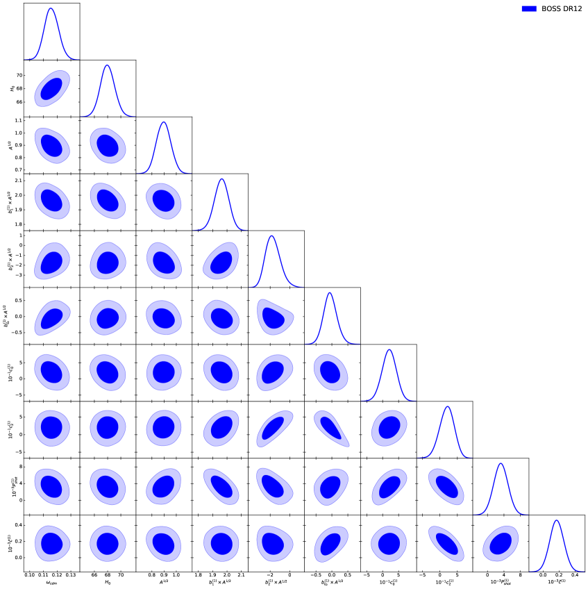
Figure 11: The posterior distribution for $\omega_{cdm},\leavevmode\nobreak\ H_{0},\leavevmode\nobreak\ A^{1/2}\equiv(A_{s}/A_{s,\,{\rm Planck}})^{1/2}$ and the high-z NGC nuisance parameters inferred from the joint BOSS DR12 full-shape likelihood.

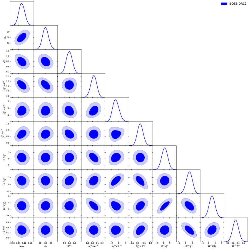
Figure 12: As Fig. 11 but for the high-z SGC region.

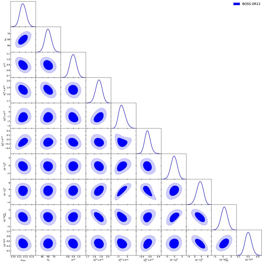
Figure 13: As Fig. 11 but for the low-z NGC region.

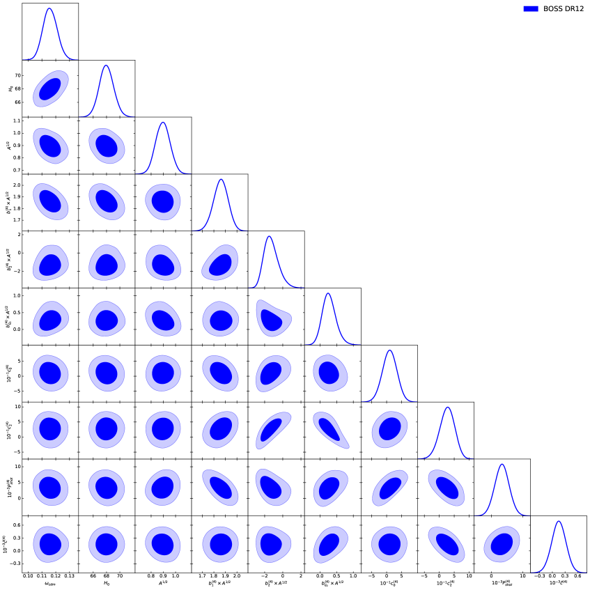
Figure 14: As Fig. 11 but for the low-z SGC region.

References

- [1] Planck collaboration, N. Aghanim et al., Planck 2018 results. VI. Cosmological parameters, 1807.06209.
- [2] U. Seljak and M. Zaldarriaga, A Line of sight integration approach to cosmic microwave background anisotropies, Astrophys. J. 469 (1996) 437 [astro-ph/9603033].
- [3] A. Lewis and S. Bridle, Cosmological parameters from CMB and other data: A Monte Carlo approach, Phys. Rev. D66 (2002) 103511 [astro-ph/0205436].
- [4] D. Blas, J. Lesgourgues and T. Tram, The Cosmic Linear Anisotropy Solving System (CLASS) II: Approximation schemes, JCAP 1107 (2011) 034 [1104.2933].
- [5] E. Bellini et al., Comparison of Einstein-Boltzmann solvers for testing general relativity, Phys. Rev. D97 (2018) 023520 [1709.09135].
- [6] T. Brinckmann and J. Lesgourgues, MontePython 3: boosted MCMC sampler and other features, Phys. Dark Univ. 24 (2019) 100260 [1804.07261].
- [7] BOSS collaboration, S. Alam et al., The clustering of galaxies in the completed SDSS-III Baryon Oscillation Spectroscopic Survey: cosmological analysis of the DR12 galaxy sample, Mon. Not. Roy. Astron. Soc. 470 (2017) 2617 [1607.03155].
- [8] EUCLID collaboration, R. Laureijs et al., Euclid Definition Study Report, 1110.3193.
- [9] L. Amendola et al., Cosmology and fundamental physics with the Euclid satellite, Living Rev. Rel. 21 (2018) 2 [1606.00180].
- [10] DESI collaboration, A. Aghamousa et al., The DESI Experiment Part I: Science,Targeting, and Survey Design, 1611.00036.
- [11] R. Takahashi, M. Sato, T. Nishimichi, A. Taruya and M. Oguri, Revising the Halofit Model for the Nonlinear Matter Power Spectrum, Astrophys. J. 761 (2012) 152 [1208.2701].
- [12] B. Audren, J. Lesgourgues, K. Benabed and S. Prunet, Conservative Constraints on Early Cosmology: an illustration of the Monte Python cosmological parameter inference code, JCAP 1302 (2013) 001 [1210.7183].
- [13] M. M. Ivanov, M. Simonovic and M. Zaldarriaga, Cosmological Parameters from the BOSS Galaxy Power Spectrum, 1909.05277.
- [14] M. M. Ivanov, M. Simonović and M. Zaldarriaga, Cosmological Parameters and Neutrino Masses from the Final Planck and Full-Shape BOSS Data, 1912.08208.
- [15] O. H. E. Philcox, M. M. Ivanov, M. Simonović and M. Zaldarriaga, Combining Full-Shape and BAO Analyses of Galaxy Power Spectra: A 1.6% CMB-independent constraint on H0, 2002.04035.
- [16] T. Nishimichi, G. D’Amico, M. M. Ivanov, L. Senatore, M. Simonovic, M. Takada et al., Blinded challenge for precision cosmology with large-scale structure: results from effective field theory for the redshift-space galaxy power spectrum, 2003.08277.
- [17] A. Chudaykin and M. M. Ivanov, Measuring neutrino masses with large-scale structure: Euclid forecast with controlled theoretical error, JCAP 1911 (2019) 034 [1907.06666].
- [18] J. Carlson, M. White and N. Padmanabhan, A critical look at cosmological perturbation theory techniques, Phys. Rev. D80 (2009) 043531 [0905.0479].
- [19] S. Tassev, N-point Statistics of Large-Scale Structure in the Zel’dovich Approximation, JCAP 1406 (2014) 012 [1311.6316].
- [20] D. Bertolini, K. Schutz, M. P. Solon, J. R. Walsh and K. M. Zurek, Non-Gaussian Covariance of the Matter Power Spectrum in the Effective Field Theory of Large Scale Structure, Phys. Rev. D93 (2016) 123505 [1512.07630].
- [21] M. Schmittfull, Z. Vlah and P. McDonald, Fast large scale structure perturbation theory using one-dimensional fast Fourier transforms, Phys. Rev. D 93 (2016) 103528 [1603.04405].
- [22] J. E. McEwen, X. Fang, C. M. Hirata and J. A. Blazek, FAST-PT: a novel algorithm to calculate convolution integrals in cosmological perturbation theory, JCAP 1609 (2016) 015 [1603.04826].
- [23] X. Fang, J. A. Blazek, J. E. McEwen and C. M. Hirata, FAST-PT II: an algorithm to calculate convolution integrals of general tensor quantities in cosmological perturbation theory, JCAP 1702 (2017) 030 [1609.05978].
- [24] M. Simonović, T. Baldauf, M. Zaldarriaga, J. J. Carrasco and J. A. Kollmeier, Cosmological perturbation theory using the FFTLog: formalism and connection to QFT loop integrals, JCAP 1804 (2018) 030 [1708.08130].
- [25] G. D’Amico, L. Senatore and P. Zhang, Limits on CDM from the EFTofLSS with the PyBird code, 2003.07956.
- [26] Y. B. Zel’Dovich, Reprint of 1970A&A…..5…84Z. Gravitational instability: an approximate theory for large density perturbations., Astronomy and Astrophysics 500 (1970) 13.
- [27] R. Scoccimarro and J. Frieman, Loop corrections in nonlinear cosmological perturbation theory, Astrophys. J. Suppl. 105 (1996) 37 [astro-ph/9509047].
- [28] R. Scoccimarro and J. Frieman, Loop corrections in nonlinear cosmological perturbation theory 2. Two point statistics and selfsimilarity, Astrophys. J. 473 (1996) 620 [astro-ph/9602070].
- [29] R. Scoccimarro, S. Colombi, J. N. Fry, J. A. Frieman, E. Hivon and A. Melott, Nonlinear evolution of the bispectrum of cosmological perturbations, Astrophys. J. 496 (1998) 586 [astro-ph/9704075].
- [30] F. Bernardeau, S. Colombi, E. Gaztanaga and R. Scoccimarro, Large scale structure of the universe and cosmological perturbation theory, Phys. Rept. 367 (2002) 1 [astro-ph/0112551].
- [31] M. Crocce and R. Scoccimarro, Renormalized cosmological perturbation theory, Phys. Rev. D 73 (2006) 063519 [astro-ph/0509418].
- [32] D. Blas, M. Garny and T. Konstandin, Cosmological perturbation theory at three-loop order, JCAP 1401 (2014) 010 [1309.3308].
- [33] M. Crocce and R. Scoccimarro, Memory of initial conditions in gravitational clustering, Phys. Rev. D 73 (2006) 063520 [astro-ph/0509419].
- [34] M. McQuinn and M. White, Cosmological perturbation theory in 1+1 dimensions, JCAP 01 (2016) 043 [1502.07389].
- [35] D. Baumann, A. Nicolis, L. Senatore and M. Zaldarriaga, Cosmological Non-Linearities as an Effective Fluid, JCAP 1207 (2012) 051 [1004.2488].
- [36] J. J. M. Carrasco, M. P. Hertzberg and L. Senatore, The Effective Field Theory of Cosmological Large Scale Structures, JHEP 09 (2012) 082 [1206.2926].
- [37] J. J. M. Carrasco, S. Foreman, D. Green and L. Senatore, The Effective Field Theory of Large Scale Structures at Two Loops, JCAP 07 (2014) 057 [1310.0464].
- [38] T. Baldauf, M. Mirbabayi, M. Simonović and M. Zaldarriaga, LSS constraints with controlled theoretical uncertainties, 1602.00674.
- [39] M. Peloso and M. Pietroni, Galilean invariance and the consistency relation for the nonlinear squeezed bispectrum of large scale structure, JCAP 05 (2013) 031 [1302.0223].
- [40] A. Kehagias and A. Riotto, Symmetries and Consistency Relations in the Large Scale Structure of the Universe, Nucl. Phys. B 873 (2013) 514 [1302.0130].
- [41] P. Creminelli, J. Noreña, M. Simonović and F. Vernizzi, Single-Field Consistency Relations of Large Scale Structure, JCAP 12 (2013) 025 [1309.3557].
- [42] D. J. Eisenstein, H.-j. Seo and M. J. White, On the Robustness of the Acoustic Scale in the Low-Redshift Clustering of Matter, Astrophys. J. 664 (2007) 660 [astro-ph/0604361].
- [43] M. Crocce and R. Scoccimarro, Nonlinear Evolution of Baryon Acoustic Oscillations, Phys. Rev. D77 (2008) 023533 [0704.2783].
- [44] N. S. Sugiyama and D. N. Spergel, How does non-linear dynamics affect the baryon acoustic oscillation?, JCAP 1402 (2014) 042 [1306.6660].
- [45] L. Senatore and M. Zaldarriaga, The IR-resummed Effective Field Theory of Large Scale Structures, JCAP 1502 (2015) 013 [1404.5954].
- [46] T. Baldauf, M. Mirbabayi, M. Simonović and M. Zaldarriaga, Equivalence Principle and the Baryon Acoustic Peak, Phys. Rev. D92 (2015) 043514 [1504.04366].
- [47] Z. Vlah, U. Seljak, M. Y. Chu and Y. Feng, Perturbation theory, effective field theory, and oscillations in the power spectrum, JCAP 1603 (2016) 057 [1509.02120].
- [48] D. Blas, M. Garny, M. M. Ivanov and S. Sibiryakov, Time-Sliced Perturbation Theory for Large Scale Structure I: General Formalism, JCAP 1607 (2016) 052 [1512.05807].
- [49] D. Blas, M. Garny, M. M. Ivanov and S. Sibiryakov, Time-Sliced Perturbation Theory II: Baryon Acoustic Oscillations and Infrared Resummation, JCAP 1607 (2016) 028 [1605.02149].
- [50] L. Senatore and G. Trevisan, On the IR-Resummation in the EFTofLSS, JCAP 1805 (2018) 019 [1710.02178].
- [51] M. M. Ivanov and S. Sibiryakov, Infrared Resummation for Biased Tracers in Redshift Space, JCAP 1807 (2018) 053 [1804.05080].
- [52] M. Lewandowski and L. Senatore, An analytic implementation of the IR-resummation for the BAO peak, JCAP 03 (2020) 018 [1810.11855].
- [53] P. McDonald and A. Roy, Clustering of dark matter tracers: generalizing bias for the coming era of precision LSS, JCAP 0908 (2009) 020 [0902.0991].
- [54] V. Assassi, D. Baumann, D. Green and M. Zaldarriaga, Renormalized Halo Bias, JCAP 1408 (2014) 056 [1402.5916].
- [55] L. Senatore, Bias in the Effective Field Theory of Large Scale Structures, JCAP 1511 (2015) 007 [1406.7843].
- [56] M. Lewandowski, A. Perko and L. Senatore, Analytic Prediction of Baryonic Effects from the EFT of Large Scale Structures, JCAP 1505 (2015) 019 [1412.5049].
- [57] M. Mirbabayi, F. Schmidt and M. Zaldarriaga, Biased Tracers and Time Evolution, JCAP 1507 (2015) 030 [1412.5169].
- [58] V. Desjacques, D. Jeong and F. Schmidt, Large-Scale Galaxy Bias, Phys. Rept. 733 (2018) 1 [1611.09787].
- [59] L. Senatore and M. Zaldarriaga, Redshift Space Distortions in the Effective Field Theory of Large Scale Structures, 1409.1225.
- [60] A. Perko, L. Senatore, E. Jennings and R. H. Wechsler, Biased Tracers in Redshift Space in the EFT of Large-Scale Structure, 1610.09321.
- [61] T. Matsubara, Resumming Cosmological Perturbations via the Lagrangian Picture: One-loop Results in Real Space and in Redshift Space, Phys. Rev. D77 (2008) 063530 [0711.2521].
- [62] R. A. Porto, L. Senatore and M. Zaldarriaga, The Lagrangian-space Effective Field Theory of Large Scale Structures, JCAP 1405 (2014) 022 [1311.2168].
- [63] J. Carlson, B. Reid and M. White, Convolution Lagrangian perturbation theory for biased tracers, Mon. Not. Roy. Astron. Soc. 429 (2013) 1674 [1209.0780].
- [64] Z. Vlah, M. White and A. Aviles, A Lagrangian effective field theory, JCAP 09 (2015) 014 [1506.05264].
- [65] Z. Vlah, E. Castorina and M. White, The Gaussian streaming model and convolution Lagrangian effective field theory, JCAP 12 (2016) 007 [1609.02908].
- [66] C. Modi, M. White and Z. Vlah, Modeling CMB lensing cross correlations with CLEFT, JCAP 08 (2017) 009 [1706.03173].
- [67] M. Schmittfull, M. Simonović, V. Assassi and M. Zaldarriaga, Modeling Biased Tracers at the Field Level, Phys. Rev. D 100 (2019) 043514 [1811.10640].
- [68] T. Baldauf, L. Mercolli and M. Zaldarriaga, Effective field theory of large scale structure at two loops: The apparent scale dependence of the speed of sound, Phys. Rev. D92 (2015) 123007 [1507.02256].
- [69] M. Pietroni, Flowing with Time: a New Approach to Nonlinear Cosmological Perturbations, JCAP 0810 (2008) 036 [0806.0971].
- [70] M. Fasiello and Z. Vlah, Nonlinear fields in generalized cosmologies, Phys. Rev. D94 (2016) 063516 [1604.04612].
- [71] L. F. de la Bella, D. Regan, D. Seery and S. Hotchkiss, The matter power spectrum in redshift space using effective field theory, JCAP 1711 (2017) 039 [1704.05309].
- [72] M. Lewandowski, L. Senatore, F. Prada, C. Zhao and C.-H. Chuang, EFT of large scale structures in redshift space, Phys. Rev. D 97 (2018) 063526 [1512.06831].
- [73] J. C. Jackson, Fingers of God: A critique of Rees’ theory of primoridal gravitational radiation, Mon. Not. Roy. Astron. Soc. 156 (1972) 1P [0810.3908].
- [74] N. Kaiser, Clustering in real space and in redshift space, Mon. Not. Roy. Astron. Soc. 227 (1987) 1.
- [75] G. D’Amico, J. Gleyzes, N. Kokron, D. Markovic, L. Senatore, P. Zhang et al., The Cosmological Analysis of the SDSS/BOSS data from the Effective Field Theory of Large-Scale Structure, 1909.05271.
- [76] M. Davis, M. J. Geller and J. Huchra, The local mean mass density of the universe: new methods for studying galaxy clustering., Astrophys. J. 221 (1978) 1.
- [77] T. Matsubara and Y. Suto, Cosmological redshift distortion of correlation functions as a probe of the density parameter and the cosmological constant, Astrophys. J. 470 (1996) L1 [astro-ph/9604142].
- [78] W. Ballinger, J. Peacock and A. Heavens, Measuring the cosmological constant with redshift surveys, Mon. Not. Roy. Astron. Soc. 282 (1996) 877 [astro-ph/9605017].
- [79] A. Heinesen, C. Blake, Y.-Z. Li and D. L. Wiltshire, Baryon acoustic oscillation methods for generic curvature: Application to the SDSS-III Baryon Oscillation Spectroscopic Survey, JCAP 1903 (2019) 003 [1811.11963].
- [80] A. Heinesen, C. Blake and D. L. Wiltshire, Quantifying the accuracy of the Alcock-Paczyński scaling of baryon acoustic oscillation measurements, JCAP 2001 (2020) 038 [1908.11508].
- [81] C. Alcock and B. Paczynski, An evolution free test for non-zero cosmological constant, Nature 281 (1979) 358.
- [82] N. Schöneberg, M. Simonović, J. Lesgourgues and M. Zaldarriaga, Beyond the traditional Line-of-Sight approach of cosmological angular statistics, JCAP 1810 (2018) 047 [1807.09540].
- [83] A. J. S. Hamilton, Uncorrelated modes of the nonlinear power spectrum, Mon. Not. Roy. Astron. Soc. 312 (2000) 257 [astro-ph/9905191].
- [84] M. Schmittfull and Z. Vlah, FFT-PT: Reducing the two-loop large-scale structure power spectrum to low-dimensional radial integrals, Phys. Rev. D94 (2016) 103530 [1609.00349].
- [85] Z. Slepian, On Decoupling the Integrals of Cosmological Perturbation Theory, 1812.02728.
- [86] J. Hamann, S. Hannestad, J. Lesgourgues, C. Rampf and Y. Y. Y. Wong, Cosmological parameters from large scale structure - geometric versus shape information, JCAP 1007 (2010) 022 [1003.3999].
- [87] D. Blas, M. Garny, T. Konstandin and J. Lesgourgues, Structure formation with massive neutrinos: going beyond linear theory, JCAP 1411 (2014) 039 [1408.2995].
- [88] L. Senatore and M. Zaldarriaga, The Effective Field Theory of Large-Scale Structure in the presence of Massive Neutrinos, 1707.04698.
- [89] F. Villaescusa-Navarro, F. Marulli, M. Viel, E. Branchini, E. Castorina, E. Sefusatti et al., Cosmology with massive neutrinos I: towards a realistic modeling of the relation between matter, haloes and galaxies, JCAP 1403 (2014) 011 [1311.0866].
- [90] E. Castorina, E. Sefusatti, R. K. Sheth, F. Villaescusa-Navarro and M. Viel, Cosmology with massive neutrinos II: on the universality of the halo mass function and bias, JCAP 1402 (2014) 049 [1311.1212].
- [91] M. Costanzi, F. Villaescusa-Navarro, M. Viel, J.-Q. Xia, S. Borgani, E. Castorina et al., Cosmology with massive neutrinos III: the halo mass function andan application to galaxy clusters, JCAP 1312 (2013) 012 [1311.1514].
- [92] E. Castorina, C. Carbone, J. Bel, E. Sefusatti and K. Dolag, DEMNUni: The clustering of large-scale structures in the presence of massive neutrinos, JCAP 1507 (2015) 043 [1505.07148].
- [93] F. Villaescusa-Navarro, A. Banerjee, N. Dalal, E. Castorina, R. Scoccimarro, R. Angulo et al., The imprint of neutrinos on clustering in redshift-space, Astrophys. J. 861 (2018) 53 [1708.01154].
- [94] A. Raccanelli, L. Verde and F. Villaescusa-Navarro, Biases from neutrino bias: to worry or not to worry?, Mon. Not. Roy. Astron. Soc. 483 (2019) 734 [1704.07837].
- [95] S. Vagnozzi, T. Brinckmann, M. Archidiacono, K. Freese, M. Gerbino, J. Lesgourgues et al., Bias due to neutrinos must not uncorrect’d go, JCAP 1809 (2018) 001 [1807.04672].
- [96] M. LoVerde, Neutrino mass without cosmic variance, Phys. Rev. D93 (2016) 103526 [1602.08108].
- [97] V. Poulin, T. L. Smith, T. Karwal and M. Kamionkowski, Early Dark Energy Can Resolve The Hubble Tension, Phys. Rev. Lett. 122 (2019) 221301 [1811.04083].
- [98] M. M. Ivanov, E. McDonough, J. C. Hill, M. Simonović, M. W. Toomey, S. Alexander et al., Constraining Early Dark Energy with Large-Scale Structure, 2006.11235.
- [99] G. D’Amico, L. Senatore, P. Zhang and H. Zheng, The Hubble Tension in Light of the Full-Shape Analysis of Large-Scale Structure Data, 2006.12420.
- [100] M. Crisostomi, M. Lewandowski and F. Vernizzi, Consistency relations for large-scale structure in modified gravity and the matter bispectrum, 1909.07366.
- [101] M. Lewandowski, Violation of the consistency relations for large-scale structure with dark energy, 1912.12292.
- [102] A. Lewis and A. Challinor, Weak gravitational lensing of the CMB, Phys. Rept. 429 (2006) 1 [astro-ph/0601594].
- [103] BOSS collaboration, F. Beutler et al., The clustering of galaxies in the completed SDSS-III Baryon Oscillation Spectroscopic Survey: baryon acoustic oscillations in the Fourier space, Mon. Not. Roy. Astron. Soc. 464 (2017) 3409 [1607.03149].
- [104] BOSS collaboration, F. Beutler et al., The clustering of galaxies in the completed SDSS-III Baryon Oscillation Spectroscopic Survey: Anisotropic galaxy clustering in Fourier-space, Mon. Not. Roy. Astron. Soc. 466 (2017) 2242 [1607.03150].
- [105] M. Tegmark, Measuring cosmological parameters with galaxy surveys, Phys. Rev. Lett. 79 (1997) 3806 [astro-ph/9706198].
- [106] M. Tegmark, A. J. Hamilton, M. A. Strauss, M. S. Vogeley and A. S. Szalay, Measuring the galaxy power spectrum with future redshift surveys, Astrophys. J. 499 (1998) 555 [astro-ph/9708020].
- [107] SDSS collaboration, M. Tegmark et al., The 3-D power spectrum of galaxies from the SDSS, Astrophys. J. 606 (2004) 702 [astro-ph/0310725].
- [108] 2dFGRS collaboration, S. Cole et al., The 2dF Galaxy Redshift Survey: Power-spectrum analysis of the final dataset and cosmological implications, Mon. Not. Roy. Astron. Soc. 362 (2005) 505 [astro-ph/0501174].
- [109] C. Blake, A. Collister, S. Bridle and O. Lahav, Cosmological baryonic and matter densities from 600,000 SDSS Luminous Red Galaxies with photometric redshifts, Mon. Not. Roy. Astron. Soc. 374 (2007) 1527 [astro-ph/0605303].
- [110] W. J. Percival et al., The shape of the SDSS DR5 galaxy power spectrum, Astrophys. J. 657 (2007) 645 [astro-ph/0608636].
- [111] BOSS collaboration, F. Beutler et al., The clustering of galaxies in the SDSS-III Baryon Oscillation Spectroscopic Survey: Testing gravity with redshift-space distortions using the power spectrum multipoles, Mon. Not. Roy. Astron. Soc. 443 (2014) 1065 [1312.4611].
- [112] A. Font-Ribera, P. McDonald, N. Mostek, B. A. Reid, H.-J. Seo and A. Slosar, DESI and other dark energy experiments in the era of neutrino mass measurements, JCAP 05 (2014) 023 [1308.4164].
- [113] J. Lesgourgues and S. Pastor, Massive neutrinos and cosmology, Phys. Rept. 429 (2006) 307 [astro-ph/0603494].
- [114] A. Lewis, Efficient sampling of fast and slow cosmological parameters, Phys. Rev. D87 (2013) 103529 [1304.4473].
- [115] A. Lewis, GetDist: a Python package for analysing Monte Carlo samples, 1910.13970.
- [116] Planck collaboration, N. Aghanim et al., Planck 2018 results. V. CMB power spectra and likelihoods, 1907.12875.
- [117] V. Desjacques, D. Jeong and F. Schmidt, The Galaxy Power Spectrum and Bispectrum in Redshift Space, JCAP 1812 (2018) 035 [1806.04015].
- [118] T. Lazeyras and F. Schmidt, Beyond LIMD bias: a measurement of the complete set of third-order halo bias parameters, JCAP 1809 (2018) 008 [1712.07531].
- [119] T. Baldauf, U. s. Seljak, R. E. Smith, N. Hamaus and V. Desjacques, Halo stochasticity from exclusion and nonlinear clustering, Phys. Rev. D 88 (2013) 083507 [1305.2917].
- [120] C. Hahn, R. Scoccimarro, M. R. Blanton, J. L. Tinker and S. A. Rodríguez-Torres, The effect of fibre collisions on the galaxy power spectrum multipoles, Mon. Not. Roy. Astron. Soc. 467 (2017) 1940 [1609.01714].
- [121] F.-S. Kitaura et al., The clustering of galaxies in the SDSS-III Baryon Oscillation Spectroscopic Survey: mock galaxy catalogues for the BOSS Final Data Release, Mon. Not. Roy. Astron. Soc. 456 (2016) 4156 [1509.06400].
- [122] H. Gil-Marín, J. Noreña, L. Verde, W. J. Percival, C. Wagner, M. Manera et al., The power spectrum and bispectrum of SDSS DR11 BOSS galaxies – I. Bias and gravity, Mon. Not. Roy. Astron. Soc. 451 (2015) 539 [1407.5668].
- [123] H. Gil-Marín, L. Verde, J. Noreña, A. J. Cuesta, L. Samushia, W. J. Percival et al., The power spectrum and bispectrum of SDSS DR11 BOSS galaxies – II. Cosmological interpretation, Mon. Not. Roy. Astron. Soc. 452 (2015) 1914 [1408.0027].