Scaling of the Formation Probabilities and Universal Boundary Entropies in the Quantum XY Spin Chain

F. Ares¹, M. A. Rajabpour², J. Viti^1,3,4,

We calculate exactly the probability to find the ground state of the XY chain in a given spin configuration in the transverse $\sigma^{z}$-basis. By determining finite-volume corrections to the probabilities for a wide variety of configurations, we obtain the universal Boundary Entropy at the critical point. The latter is a benchmark of the underlying Boundary Conformal Field Theory characterizing each quantum state. To determine the scaling of the probabilities, we prove a theorem that expresses, in a factorized form, the eigenvalues of a sub-matrix of a circulant matrix as functions of the eigenvalues of the original matrix. Finally, the Boundary Entropies are computed by exploiting a generalization of the Euler-MacLaurin formula to non-differentiable functions. It is shown that, in some cases, the spin configuration can flow to a linear superposition of Cardy states. Our methods and tools are rather generic and can be applied to all the periodic quantum chains which map to free-fermionic Hamiltonians.

 

 

I Introduction

The ground state of a quantum spin chain is usually a complicated state which, when written on a local basis, expands over an exponential number of terms. Each term in the expansion corresponds to a spin configuration on the selected basis. Simultaneous measurements of all the local spins project the ground state into a single spin configuration with a certain probability, which is the absolute value squared of the overlap between such a state and the chosen configuration. The same is true for a spinless fermionic system on a lattice, where the measurement leads to a configuration whose lattice sites may or not be occupied by a fermion.

It is also possible to perform projective measurements on a subsystem. The simplest instance is perhaps the probability to observe the totality of the spins on a finite interval of the chain pointing up or down, which is the so-called Emptiness Formation Probability. Such a quantity has been calculated analytically in a few integrable quantum chains, see Korepin:1994ui ; Essler:1994se ; Essler:1995vp ; shiroishi2001emptiness ; Kitanine2002a ; Korepin2003 ; FA ; Painleve . In the scaling limit, next to a critical point, the Emptiness Formation Probability can be interpreted as statistical mechanics partition function on a cylinder or a strip with suitable boundary conditions Stephan2013 . Within this formulation, it can be studied by applying Quantum Field Theory (QFT) and Conformal Field Theory (CFT) techniques, see also Rajabpour2015 ; Rajabpour2016 ; Viti2016 . In particular, at criticality one can extract universal data such as the central charge Stephan2013 of the underlying CFT and the anomalous dimensions of all the scaling fields Rajabpour2015 . A string of fully polarized spins is however just one example among the possible configurations that can be fixed for the subsystem. The probability of finding a finite portion of the ground state in a generic spin configuration has been also studied numerically in najafi2016formation ; Najafi:2019ypm and dubbed Formation Probability (FP). Similar connections to CFT can be drawn for a wide variety of FPs najafi2016formation .

FPs can be of course defined also for the whole spin chain, in this case they coincide with the absolute value squared of the ground state overlaps.

Analogously, it is expected that at criticality the $O(1)$ correction to their large volume expansion is universal and given by the Boundary Entropy (BE) introduced in boundary . For similar studies in the scaling limit with integrability techniques, we refer to LeClair1994 ; Dorey1998 ; Dorey2000 ; Friedan2004 ; Dorey2004 ; Pozsgay2010 ; Caetano2020 . By determining the BEs, one can infer the fixed point of the renormalization group flow, i.e. the conformal boundary state, attracting at large scales any spin configurations Cardy_Sci . Renormalization of the ground state of a perturbed CFT toward a conformal boundary state is also a key assumption for the approach to non-equilibrium phenomena initiated in CC . Finite size corrections to the FPs for completely polarized states in the XY and XXZ chain have been discussed in Wei2005 ; Stephan2009 ; Huang2010 ; Stephan2010 and Shi2010 ; Stephan2010b ; SB respectively. Overlaps in gapless spin chain with central charge one, have been studied in CS . These analyses were also relevant to understand whether geometric entanglement could serve as a possible measure of multipartite entanglement Barnum2001 ; Wei2003 .

Although the ground state overlaps—alias the FPs—seem fundamental building blocks of a quantum many-body theory, they have not been extensively investigated.

In this paper, we try to make the first steps toward a systematic study. We focus on the the quantum XY chain and determine the FPs in the transverse $\sigma^{z}$-basis for a wide variety of spin configurations. After computing exactly their asymptotic behaviour for large volume, we are able to extract the subleading volume-independent contribution and point out the boundary CFT characterizing each configuration.

Our methods and tools are quite generic and can be applied to any system that maps to a periodic quadratic fermionic Hamiltonian. On the technical side, first, we prove a novel result for circulant matrices which allows us to obtain a closed finite-size expression for the FPs. Then we exploit the Euler-MacLaurin (EM) summation formulas to determine their large volume expansion. To calculate the BE, in particular, we recall a nice generalization of the EM famous theorem, which can be applied also to non-differentiable functions Navot1 ; Navot2 .

The rest of the paper is organized as follows: in Sec. II we derive field theoretical predictions for the FPs in the XY chain and write down an explicit determinant representation for them; in Sec. III, we illustrate applications of the formalism to the fully polarized states and the Néel state; in Sec. IV, FPs are determined, together with their asymptotic behaviour in the large volume limit, for a wide class of states in the XY chain; in Sec. V, we focus on the XX chain and conclude in Sec. VI. The paper has also three Appendices. Appendix A adapts the results of Navot2 to the XY chain; Appendix B contains a proof of the main technical novelty of this paper, namely a closed expression for the determinant of a sub-matrix of a circulant matrix. Finally, Appendix C adds some details to the examples examined in Sec. IV.

II Formation Probabilities and Boundary Entropies in the XY chain

Boundary Entropies at a Quantum Critical Point.—We start by introducing the XY spin chain in a transverse field $h$, defined by the Hamiltonian Lieb

$$H_{\text{XY}}=-\frac{1}{2}\sum_{n=1}^{L}\left[\frac{1+\gamma}{2}~{}\sigma^{x}_{n}\sigma^{x}_{n+1}+\frac{1-\gamma}{2}~{}\sigma^{y}_{n}\sigma^{y}_{n+1}+h\sigma_{n}^{z}\right],$$ (1)

where $\sigma_{n}^{\alpha}$ ($\alpha=1,2,3$) are Pauli matrices satisfying $[\sigma^{\alpha}_{n},\sigma^{\beta}_{m}]=2i\varepsilon^{\alpha\beta\nu}\delta_{n,m}\sigma^{\nu}_{n}$ and the parameter $\gamma$ is dubbed anisotropy. We furthermore assume periodic boundary conditions for the spins, namely $\sigma_{n}^{\alpha}=\sigma_{n+L}^{\alpha}$, and restrict ourselves to $L=2N$ even. The Hamiltonian in Eq. (1) commutes with the parity operator

$$P=\prod_{n=1}^{L}\sigma_{n}^{z},$$ (2)

whose eigenvalues are $\mathcal{N}=\pm 1$. $P$ implements the $\mathbb{Z}_{2}$ symmetry of the model under spin flip in the $x$-direction. The Hilbert space splits into a direct sum of two subspaces: that containing linear combinations of states with an odd number of down spins along the $z$-direction, the so-called Ramond (R) sector with $\mathcal{N}=-1$, and the one containing states with an even number of down spins, or Neveu-Schwarz (NS) sector, where $\mathcal{N}=1$. Both subspaces have dimension $2^{L-1}$. In the region of the phase space $h^{2}+\gamma^{2}>1$, the ground state of the XY chain, which will be denoted by $|\Omega\rangle$, belongs to the NS sector Katsura ; DR ; OYNR and we will examine only this possibility from now on. The ground state energy is

$$E_{\text{gs}}=-\frac{1}{2}\sum_{k=1}^{L}\varepsilon(\phi_{k}),$$ (3)

where $\varepsilon(\phi)=\sqrt{(h-\cos\phi)^{2}+\gamma^{2}\sin^{2}\phi}$ and $\phi_{k}=\frac{2\pi}{L}(k-1/2)$ with $k=1,\dots,L$. Inside the circle $h^{2}+\gamma^{2}<1$, the lowest energy state oscillates between the R and NS sector and the analysis is more involved. In particular, the case $\gamma=0$ and $|h|<1$ will be discussed separately in Sec. V. The energy gap of the XY chain OYNR closes as $O(L^{-1})$ along the critical lines $|h|=1$ and $\gamma\not=0$. The low-energy quasi-particle excitations are free Majorana fermions described by a CFT with central charge $c=1/2$: this is the Ising CFT. In the Majorana fermion language, the NS sector is spanned by states that contain only an even number of fermionic quasi-particles.

Take an element of the $\sigma^{z}$-basis, $|\boldsymbol{\sigma}\rangle\equiv|\bullet_{1}\bullet_{2}\dots\bullet_{2N}\rangle$ with $\bullet_{n}\in\{|\uparrow\rangle_{n},|\downarrow\rangle_{n}\}$, an eigenvector of the local operators $\sigma_{n}^{z}$ associated to the eigenvalues $\pm 1$. Consider then in the XY chain the amplitude

$$f_{\boldsymbol{\sigma}}(\beta,L)\equiv\langle\boldsymbol{\sigma}|e^{-\beta H_{\text{XY}}}|\boldsymbol{\sigma}\rangle,$$ (4)

in the limit $\beta\gg L\gg 1$; Eq. (4) could be also interpreted as the Return Amplitude RA analytically continued to imaginary times.

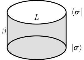
Figure 1: The conformal partition functions on a annulus of circumference $L$ and height $\beta$. The state $|\boldsymbol{\sigma}\rangle$ acts as a boundary condition for the vertical imaginary time evolution. Rotating the annulus by $90$ degrees such a partition function can be interpreted as the conformal partition function of a system of finite length $\beta$ with temperature $1/L$. Imaginary time evolution happens now around the cylinder. In such a case the spins at edges should be described by a conformal invariant boundary condition Cardyboundary .

Inserting a complete set of states, up to exponentially small corrections in the inverse temperature, one has

$$f_{\boldsymbol{\sigma}}(\beta,L)\stackrel{{\scriptstyle\beta\gg L\gg 1}}{{\longrightarrow}}|\langle\boldsymbol{\sigma}|\Omega\rangle|^{2}e^{-\beta E_{\text{gs}}},$$ (5)

where $E_{\text{gs}}$ is the ground state energy in Eq. (3). For $L\gg 1$, the ground states overlap is expected to decay exponentially with a possible $O(1)$ term

$$\log|\langle\boldsymbol{\sigma}|\Omega\rangle|^{2}=-\Gamma_{\boldsymbol{\sigma}}L+2s_{\boldsymbol{\sigma}}+O(1/L),$$ (6)

while extensivity of the ground state energy requires

$$E_{\text{gs}}=uL+u^{\prime}-\frac{b}{L}+O(1/L^{2}).$$ (7)

The coefficients $s_{\boldsymbol{\sigma}}$ and $b$ in the large volume expansions in Eqs. (6, 7) are dimensionless and argued to be universal, namely lattice-spacing independent, in the scaling limit. They can be calculated within a QFT formalism. Indeed, the amplitude in Eq. (4) can be interpreted as a partition function on the annulus depicted in Fig. 1. At criticality, the bulk theory is conformal invariant and the state $|\boldsymbol{\sigma}\rangle$ acts as a boundary condition for the vertical imaginary time evolution. The latter is driven by the bulk conformal Hamiltonian with central charge $c$. If the state $|\boldsymbol{\sigma}\rangle$ coincides with the ground state of a massive deformation of a CFT Cardy_Sci , at the bulk critical point, it renormalizes toward a conformal boundary state $|\Phi\rangle$. In this case, the universal part of the quantum amplitude in Eq. (4), in the limit $\beta\gg L\gg 1$, is given by boundary

$$f_{\boldsymbol{\sigma}}(\beta,L)|_{\text{univ}}\stackrel{{\scriptstyle\beta\gg L\gg 1}}{{\longrightarrow}}g_{\Phi}^{2}~{}e^{\frac{\beta}{L}\frac{\pi cv_{F}}{6}},$$ (8)

where $v_{F}$ is the Fermi velocity and $g_{\Phi}\equiv\langle\Phi|\Omega\rangle>0$ is the renormalized Boundary Entropy (BE) boundary . In the following, we will examine spin configurations $|\boldsymbol{\sigma}\rangle$ that exhibit a periodic pattern of period $p\ll L$ in real space and conjecture that for large volume they are still attracted by a conformal boundary state $|\Phi\rangle$. Our analysis, in particular, does not cover the possibility of states that break translation invariance in the continuum limit, such as the domain wall $|\boldsymbol{\sigma}\rangle=|\overbrace{\uparrow\uparrow\dots\uparrow}^{L/2}\overbrace{\downarrow\dots\downarrow\downarrow}^{L/2}\rangle$ and which deserve a separate study Ref1 . Eq. (8) implies the celebrated Cardyfree ; Affleckfree universality of the $O(1/L)$ term in the expansion of the ground state energy $b=(\pi cv_{F})/6$, see Eq. (7). For the critical XY chain, as long as $\gamma\not=0$, one has $v_{F}=\gamma$ and $c=1/2$; indeed the CFT result for $b$ can be readily checked applying the EM summation formula (43) to Eq. (3).

The notion of conformal boundary states, or Cardy states, was introduced in the seminal work Cardyboundary and nowadays is well established Cardy_Rev . Here we only mention that in the Ising CFT there are two types of boundary states, free and fixed, distinguished by $\mathbb{Z}_{2}$ symmetry. The free boundary state $|\Phi\rangle=|\text{free}\rangle$ has the property that $\langle\text{free}|\sigma_{n}^{x}|\text{free}\rangle=0$, while for fixed boundary states $|\Phi\rangle=|\pm\rangle$ one has $\langle\pm|\sigma_{n}^{x}|\pm\rangle=\pm 1$. However, if $\gamma\not=0$ and in absence of a longitudinal field coupling to $\sigma_{n}^{x}$, all the states in the NS sector, when expressed in the $\sigma^{x}$-basis, are symmetric under $\sigma^{x}_{n}\rightarrow-\sigma_{n}^{x}$. Consequently, any spin configuration $|\boldsymbol{\sigma}\rangle$ in the NS sector should renormalize either to the free boundary state or to the linear superposition with equal weights of fixed boundary states. In conclusion, field theory predicts that for $|h|=1$ the $O(1)$ term in Eq. (6) does not depend even on $\gamma$ and is given by Kon

$$s_{\boldsymbol{\sigma}}(h)|_{h=\pm 1}=\log g_{\Phi}=\left\{\begin{array}[]{l}0~{}\text{if $|\boldsymbol{\sigma}\rangle\stackrel{{\scriptstyle\text{flows to}}}{{\rightarrow}}|\Phi\rangle=|\text{free}\rangle$},\\ \frac{1}{2}\log 2~{}\text{if $|\boldsymbol{\sigma}\rangle\stackrel{{\scriptstyle\text{flows to}}}{{\rightarrow}}|\Phi\rangle=|+\rangle+|-\rangle$}.\end{array}\right.$$ (9)

The equal weight linear combination of fixed boundary states in Eq. (9) already occurred in the literature. For instance, in the study of the boundary phase diagram of the Tricritical Ising model Chim ; afflecktri ; GRW and in the analysis of the renormalization group flow of the massive ground state of the Ising spin chain Kon . As we will discuss at the end of Sec. IV, the two boundary states $|+\rangle+|-\rangle$ and $|\text{free}\rangle$ are related by Kramers-Wannier (KW) duality Kon . The interpretation of the linear superposition in terms of a topological defect GW ; Kon2 and its appearance along a boundary flow has also been recently emphasized in FI . Finally notice that in principle other $\mathbb{Z}_{2}$ symmetric linear superpositions of the fixed boundary states could appear in Eq. (9), leading to larger boundary entropies. Nevertheless, as we will discuss in detail in the next sections, our results are consistent with a renormalization toward the simplest possibility given by the state $|+\rangle+|-\rangle$.

Determinant Representation for the Overlaps.— We provide here an explicit determinant representation for the overlap $\langle\boldsymbol{\sigma}|\Omega\rangle$ in the XY chain, see Eq. (17). This is the starting point of our study of the FPs. Consider a state $|\boldsymbol{\sigma}\rangle$ with $2r$ down spins at positions: $1\leq i_{1}<i_{2}<\dots<i_{2r}\leq 2N$. By adapting to imaginary time the formalism in RA , the partition function $f_{\boldsymbol{\sigma}}(\beta,L=2N)$ in Eq. (4) can be calculated as

$$f_{\boldsymbol{\sigma}}(\beta,2N)=\frac{\text{Pf}(\textbf{M}_{\sigma}(\beta))}{\sqrt{\det(\textbf{Q}(\beta))}},$$ (10)

where the symbol Pf denotes the Pfaffian ($[\text{Pf}(\textbf{A})]^{2}=\det\textbf{A}$ for A antisymmetric). The antisymmetric matrix $\textbf{M}_{\sigma}$ is obtained from the $4N\times 4N$ antisymmetric matrix

$$\textbf{M}=\begin{bmatrix}-i\textbf{X}&\textbf{Q}\\ -\textbf{Q}&i\textbf{X}\end{bmatrix},\quad\textbf{Q}=\textbf{Q}^{\dagger},~{}\textbf{X}=\textbf{X}^{\dagger}$$ (11)

by removing the columns and rows $\{i_{1},\dots,i_{2r}\}$ and $\{i_{1}+2N,\dots,i_{2r}+2N\}$. The Hermitian matrices X and Q are circulant and commute; they are explicitly given by RA

$$[\textbf{X}(\beta)]_{lm}=\frac{1}{2N}\sum_{k=1}^{2N}\frac{\gamma\sin(\phi_{k})e^{-i\phi_{k}(l-m)}}{-h+\cos(\phi_{k})+\varepsilon(\phi_{k})\coth(\beta\varepsilon(\phi_{k}))}$$ (12)

$$[\textbf{Q}(\beta)]_{lm}=\frac{1}{2N}\sum_{k=1}^{2N}\frac{e^{-i\phi_{k}(l-m)}}{\cosh(\beta\varepsilon(\phi_{k}))+\frac{-h+\cos(\phi_{k})}{\varepsilon(\phi_{k})}\sinh(\beta\varepsilon(\phi_{k}))}.$$ (13)

In order to determine the BEs, we shall evaluate them in the limit $\beta\rightarrow\infty$. From Eq. (13) one obtains

$$\frac{1}{\sqrt{\det(\textbf{Q}(\beta))}}\stackrel{{\scriptstyle\beta\gg 1}}{{\longrightarrow}}e^{\frac{1}{2}\beta\sum_{k=1}^{2N}\varepsilon(\phi_{k})}\prod_{k=1}^{N}\left(\frac{1}{2}-\frac{h-\cos(\phi_{k})}{2\varepsilon(\phi_{k})}\right);$$ (14)

the exponential prefactor above, cf. Eqs. (3) and (5), reproduces $e^{-\beta E_{gs}}$ when $\gamma\not=0$. In the limit $\beta\rightarrow\infty$, on the other hand, Q vanishes exponentially fast and M becomes block diagonal; we can then define

$$[\textbf{W}]_{lm}\equiv\lim_{\beta\rightarrow\infty}[\textbf{X}(\beta)]_{lm}=\frac{1}{2N}\sum_{k=1}^{2N}e^{-i\phi_{k}(l-m)}w(\phi_{k}),\quad\text{with}$$ (15)

$$w(\phi_{k})\equiv\frac{\gamma\sin(\phi_{k})}{-h+\cos(\phi_{k})+\varepsilon(\phi_{k})}.$$ (16)

From Eqs. (10-11) and Eq. (5), it finally follows

$$|\langle\boldsymbol{\sigma}|\Omega\rangle|^{2}=\prod_{k=1}^{N}\left(\frac{1}{2}-\frac{h-\cos(\phi_{k})}{2\varepsilon(\phi_{k})}\right)|\det\textbf{W}_{\sigma}|,$$ (17)

where $\textbf{W}_{\sigma}$ is the matrix extracted from W, by removing the columns and rows with indices $\{i_{1},\dots,i_{2r}\}$ which are in correspondence with the positions of the down spins in the state $|\boldsymbol{\sigma}\rangle$. As a side remark, we observe that M in Eq. (11) has the same formal structure as the correlation matrix derived in FA to evaluate the Emptiness Formation Probability, see also Painleve . After a few manipulations, its Pfaffian can be rewritten as $\text{Pf}(\textbf{M})=|\det(\textbf{Q}+i\textbf{X})|$, from which Eq. (17) also follows in the $\beta\rightarrow\infty$ limit. For similar determinant expressions, we refer to Stephan2010 .

In Sec. IV, see Appendix B for a proof, will be presented a formula for $\det\textbf{W}_{\sigma}$ valid for a large class of states, which is particularly useful in the large $N$ limit.

III Fully Polarized States and the Néel State

To validate the CFT predictions in Eq. (9), we start by analyzing FP for fully polarized states and the Néel state. Although the results presented in this Section are particular cases of the general discussion of Sec. IV, we prefer to illustrate the main ideas first through these simpler examples. Results in this Section are valid for any $\gamma\not=0.$

Fully Polarized States.— For the fully polarized up state, $|\boldsymbol{\sigma}\rangle=|\uparrow\dots\uparrow\rangle$, the matrix $\textbf{W}_{\uparrow\dots\uparrow}=\textbf{W}$. By applying directly Eq. (17) we can then calculate the ground state overlap

$$\log|\langle\uparrow\dots\uparrow|\Omega\rangle|^{2}=\sum_{k=1}^{N}\log[g_{+}(\phi_{k})],$$ (18)

with $g_{+}(\phi)=\frac{1}{2}+\frac{h-\cos(\phi)}{2\varepsilon(\phi)}$. To compute the scaling with the system size of the FP, one shall apply the EM summation formula and approximate for large $N$ the sum in Eq. (18). The leading $O(N)$ contribution, cf. Eq. (6), is straightforward and $\Gamma_{\uparrow\dots\uparrow}=-\int_{0}^{\pi}\frac{d\phi}{2\pi}\log[g_{+}(\phi)]>0$. However, contrary to the ground state energy in Eq. (3), the calculation of the subleading $O(1)$ term and therefore of the BE is non-trivial. Indeed, for some values of the parameters $(h,\gamma)$ the summand as a function of $\phi\in[0,\pi]$ is not differentiable and develops logarithmic singularities.

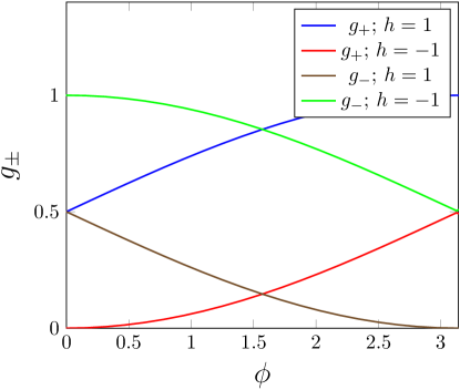
Figure 2: The argument of the logarithms in Eqs. (18-19) as a function of the angle $\phi\in[0,\pi]$ for $\gamma=1$ (Ising spin chain). $O(1)$ contributions in the large $N$ approximations of the sums in Eqs. (18-19) are produced by zeros or divergences, according to Appendix A. For fully polarized states only zeros occur with $\alpha=2$.

Interestingly Navot1 ; Navot2 , see Appendix A, logarithmic singularities are responsible for the presence of non-zero $O(1)$ terms in the large $N$ expansion. These, in turn, fix through Eq. (6) the value of the BE along the critical lines $h=\pm 1$. For instance, see also Fig. 2, at $h=1$, the function $g_{+}$ is always positive and differentiable, while vanishes quadratically at $\phi=0$, when $h=-1$. In the former case $\log[g_{+}(\phi)]$ is a smooth function and the EM summation formula (43) gives $s_{\uparrow\dots\uparrow}(h)|_{h=1}=0$, corresponding to the free boundary state, cf. Eq. (9). In the latter, instead, $\log[g_{+}(\phi)]$ is singular at the boundary of the integration domain. The extended EM summation formula (44) applies with $\alpha=2$ and leads to $s_{\uparrow\dots\uparrow}(h)|_{h=-1}=\frac{1}{2}\log 2$, which indicates renormalization toward the linear superposition of fixed boundary states. Analogous considerations are valid for the fully polarized down state $|\boldsymbol{\sigma}\rangle=|\downarrow\dots\downarrow\rangle$. There is no matrix $\textbf{W}_{\downarrow\dots\downarrow}$ in Eq. (17) and

$$\log|\langle\downarrow\dots\downarrow|\Omega\rangle|^{2}=\sum_{k=1}^{N}\log[g_{-}(\phi_{k})],$$ (19)

with $g_{-}|_{h}(\phi)=g_{+}|_{-h}(\pi-\phi)=\frac{1}{2}-\frac{h-\cos(\phi)}{2\varepsilon(\phi)}$, see also Fig. 2. In particular, the values of the BE in a fully polarized down state as a function of the transverse field are reversed with respect to those of a fully polarized up state, that is $s_{\downarrow\dots\downarrow}(h)=s_{\uparrow\dots\uparrow}(-h)$.

Néel State.— It is instructive to study separately also the Néel state, $|\boldsymbol{\sigma}\rangle=|\downarrow\uparrow\dots\downarrow\uparrow\rangle$; the state will be in the NS sector if $N$ is even; i.e. if the total length $L=2N$ of the chain is divisible by four. The matrix $\textbf{W}_{\sigma}$, in Eq. (17), is obtained by removing the odd columns and rows from W in Eq. (15). Since the smaller matrix is circulant, its eigenvalues can be computed by elementary means and from Eq. (17) one obtains

$$\log|\langle\downarrow\uparrow\dots\downarrow\uparrow|\Omega\rangle|^{2}=\sum_{k=1}^{N}\log[g_{-+}(\phi_{k})],\quad\text{with}$$ (20)

$$g_{-+}(\phi)=\frac{\gamma\sin(\phi)}{4\varepsilon(\phi)}\left|1-\frac{\varepsilon(\phi)-h+\cos(\phi)}{\varepsilon(\phi+\pi)-h-\cos(\phi)}\right|.$$ (21)

The leading term in the large $N$ expansion of Eq. (20) is $\Gamma_{\downarrow\uparrow\dots\downarrow\uparrow}=-\int_{0}^{\pi}\frac{d\phi}{2\pi}\log[g_{-+}(\phi)]$, which can be shown to be positive by direct numerical integration. The value of the $O(1)$ contribution is again set by the zeros and the singularities of the function $g_{-+}(\phi)$ with $\phi\in[0,\pi]$. For $h=1$, $g_{-+}(\phi)$ diverges as $1/\phi$ close to $\phi=0$, is not differentiable at $\phi=\pi/2$ and vanishes linearly at $\phi=\pi$. According to Appendix A and Eq. (6), one then obtains $s_{\downarrow\uparrow\dots\downarrow\uparrow}(h)|_{h=1}=\frac{1}{2}\log 2$, indicating renormalization toward the linear combination of fixed boundary states. For $h=-1$, $g_{-+}$ has only a non-differentiable point at $\phi=\pi/2$, leading again to a BE $s_{\downarrow\uparrow\dots\downarrow\uparrow}(h)|_{h=-1}=\frac{1}{2}\log 2$, consistent with the symmetry under spin flip in the $z$-direction of the Néel state. The function $g_{+-}(\phi)$ is plotted for $h=\pm 1$ and $\gamma=1$ in Fig. 3; the caption provides a few additional details on the application of Eq. (44).

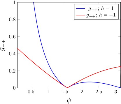
Figure 3: The function $g_{-+}(\phi)$ plotted in the domain $\phi\in[0,\pi]$ at $\gamma=1$. In order to apply the extended EM summation formula in Eq. (44), we divide the interval $[0,\pi]$ in two, adding a boundary point at $\phi=\pi/2$. For $h=1$ (blue curve) one has a singularity with $\alpha=-1$ at $\phi=0$ and three additional singularities with $\alpha=1$, two at $\phi=\pi/2$ and one at $\phi=\pi$. When $h=-1$ instead (red curve), the function $g_{-+}$ has only a non-differentiable point at $\phi=\pi/2$. In both cases, the BE is $s_{\downarrow\uparrow\dots\downarrow\uparrow}=\frac{1}{2}\log 2$, indicating a flow toward the linear combination of fixed boundary states.

IV Formation Probabilities and Boundary Entropies for Generic Spin Configurations

We now present a rather general technique to calculate the FP of eigenstates $|\boldsymbol{\sigma}\rangle$ of the local spin operators $\sigma_{n}^{z}$. This is based, see Eqs. (23-24), on a factorized expression for their overlap with the XY ground state.

Along the lines of LC , we discuss states that are obtained by repeating an elementary block $\mathcal{B}_{s,p}$ of $p$ spins; inside any block there are $s$ consecutive up spins. Conventionally and without loosing in generality, all the states except the fully polarized up state (i.e. the block $\mathcal{B}_{1,1}$) start with a down spin. For instance the Néel state, discussed in the previous Section, is labelled by the block $\mathcal{B}_{1,2}$; analogously a state such as $|\downarrow\downarrow\uparrow\uparrow\dots\downarrow\downarrow\uparrow\uparrow\rangle$ is in correspondence with the block $\mathcal{B}_{2,4}$. Defining

$$M\equiv\frac{2N}{p},$$ (22)

one then finds a total of $sM$ up spins at positions $q=jp+r$, with $j=0,\dots,M-1$ and $r=p-s+1,\dots,p$; we can further ensure that these states belong to the NS sector choosing $N$ a multiple of $p$. To determine the FPs one shall calculate the determinant in Eq. (17); in this regard, in Appendix B, we will prove the following formula

$$\det\textbf{W}_{\sigma}=\prod_{k=1}^{M}~{}\mathcal{P}_{0}\left(w(\phi_{k}),w(\phi_{k+M}),\dots,w(\phi_{k+(p-1)M})\right),$$ (23)

with $w(\phi)$ given in Eq. (16). $\mathcal{P}_{0}(x_{1},\dots,x_{p})$ in Eq. (23) is a polynomial which coincides with the first non-vanishing coefficient —that of the power of degree $(p-s)$— of the characteristic polynomial of the $p\times p$ matrix

$$[\textbf{A}]_{lm}=\frac{x_{l}}{p}\left[s~{}\delta_{l,m}-(1-\delta_{l,m})e^{\frac{i\pi(l-m)(p-s)}{p}}\frac{\sin\left(\frac{\pi(l-m)(p-s)}{p}\right)}{\sin\left(\frac{\pi(l-m)}{p}\right)}\right];\quad l,m=1,\dots,p.$$ (24)

Eqs. (23) and (17) can be then used to calculate analytically the ground state overlaps of the states $|\boldsymbol{\sigma}\rangle$, labelled by the block $\mathcal{B}_{s,p}$, as

$$\log\left|\frac{\langle\boldsymbol{\sigma}|\Omega\rangle}{\langle\downarrow\dots\downarrow|\Omega\rangle}\right|^{2}=\sum_{k=1}^{M}\log\left|\mathcal{P}_{0}(w(\phi_{k}),w(\phi_{k+M}),\dots,w(\phi_{k+M(p-1)}))\right|.$$ (25)

The coefficient $\Gamma_{\boldsymbol{\sigma}}$ in Eq. (6) ruling the leading large $N$ behaviour of the FPs is then

$$\Gamma_{\boldsymbol{\sigma}}=\Gamma_{\downarrow\dots\downarrow}+\int_{0}^{\frac{2\pi}{p}}\frac{d\phi}{2\pi}\log\bigl{|}\mathcal{P}_{0}\bigl{(}w(\phi),w(\phi+2\pi/p),\dots,w(\phi+2\pi(p-1)/p)\bigr{)}\bigr{|},$$ (26)

and from Eq. (25), the BEs are also determined in analogy to what was done in Sec. III for the fully polarized and the Néel states. We could also extend the analysis of the $O(1)$ term in the large $N$ expansion of Eq. (25) for any points outside the circle $h^{2}+\gamma^{2}=1$. Notice that, by symmetry, if $|\boldsymbol{\sigma}^{\prime}\rangle$ is obtained by flipping in the $z$-direction all the spins of $|\boldsymbol{\sigma}\rangle$, it must hold $s_{\boldsymbol{\sigma}}(h)=s_{\boldsymbol{\sigma}^{\prime}}(-h)$. The property is shared, for example, by the state $|\boldsymbol{\sigma}\rangle$, labelled by the block $\mathcal{B}_{s,p}$, and its companion $|\boldsymbol{\sigma^{\prime}}\rangle$, labelled by $\mathcal{B}_{p-s,p}$. Its verification provides a non-trivial test of the formalism.

Based on a case by case study which is reported below and in Appendix C, a pattern emerges for the BEs that will be illustrated at the end of this Section, together with a physical interpretation.

Example 1.— Consider the state associated to the block $\mathcal{B}_{s=1,p}$; this is of the form $|\overbrace{\downarrow\dots\downarrow}^{p-1}\uparrow\dots\rangle$. For $s=1$, the polynomial $\mathcal{P}_{0}(x_{1},\dots,x_{p})$ is minus the trace of the matrix A in Eq. (24); namely

$$\mathcal{P}_{0}(x_{1},\dots,x_{p})=-\frac{1}{p}\sum_{j=1}^{p}x_{j}.$$ (27)

From Eq. (25), one obtains the ground state overlap for the class of states labelled by the block $\mathcal{B}_{1,p}$

$$\log\left|\frac{\langle\boldsymbol{\sigma}|\Omega\rangle}{\langle\downarrow\dots\downarrow|\Omega\rangle}\right|^{2}=\sum_{k=1}^{2N/p}\log[g_{1,p}(\phi_{k})].$$ (28)

The function $g_{1,p}$, cf. Eq. (27), reads

$$g_{1,p}(\phi)=\frac{1}{p}\left|\sum_{j=0}^{p-1}w\left(\phi+\frac{2\pi j}{p}\right)\right|,$$ (29)

where we have further used $\phi_{k+m}=\phi_{k}+\frac{\pi m}{N}$ for any integer $m$. The same result could be derived more prosaically observing that for $s=1$ the matrix $\textbf{W}_{\sigma}$ in Eq. (47) is circulant and its eigenvalues can be calculated directly.

As explained in Sec. III, by identifying the zeros and the singularities in the interval $\phi\in[0,2\pi/p]$ of $g_{1,p}$ in Eq. (29) we can determine the BEs. We start from the line $h=1$. For $p$ even, the function $g_{1,p}(\phi)$ diverges at $\phi=0$ and $\phi=2\pi/p$, while is vanishing and non-differentiable at $\phi=\pi/p$. According to Eq. (44) there is no $O(1)$ term when approximating the sum in Eq. (28) for large $N$. By combining this result with the analysis of the analogous contribution coming from $\log|\langle\{\downarrow\}|\Omega\rangle|^{2}$ in Eq. (28), see Sec. III, we conclude that states associated to configurations $\mathcal{B}_{1,p}$ and $p$ even renormalize toward the linear superposition of fixed boundary states. Interestingly when $p$ is odd, this is no longer the case. For $p$ odd and $h=1$, the function $g_{1,p}(\phi)$ has only a pole at $\phi=\pi/p$. In the notations of Appendix A, there are then two singularities with $\alpha=-1$ and the $O(1)$ term in the large $N$ expansion of Eq. (28) has value $-\log 2$. Taking into account the contribution of the fully polarized down state, it follows that states with $p$ odd renormalize toward the free boundary state. These findings are also summarized in Fig. 4, which illustrates the universality of the BEs along the quantum critical line $h=1$.

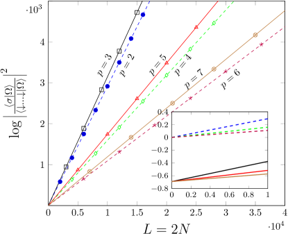
Figure 4: Direct evaluation of the sums in Eq. (28) for several values of $p$ for $h=1$ and $\gamma=1$. The straight lines are linear fits of the data obtained at different $L=2N$. The inset contains the behaviour of the straight lines close to the origin: the $O(1)$ term in large $N$ expansion of Eq. (28) is $-\log 2$ for odd $p$ (solid lines) and zero for even $p$ (dashed lines). These values follow from application of Eq. (44) and the properties of the function $g_{1,p}(\phi)$ in Eq. (29).

Finally, at $h=-1$, the function $g_{1,p}(\phi)$ for both even and odd $p$ has two singularities with $\alpha=1$ in the domain $\phi\in[0,2\pi/p]$. In such a case, there is no $O(1)$ term in Eq. (28) coming from the fully polarized down state. We then conclude that the states associated to $\mathcal{B}_{1,p}$ have BE $s_{\sigma}=\frac{1}{2}\log 2$ at $h=-1$, indicating renormalization toward the linear superposition of fixed boundary states for any $p>1$.

Example 2.— Consider now the more general states associated to the blocks $\mathcal{B}_{s,p}$ for $s>1$. For the sake of brevity, we sketch out two examples with $p=4$ and defer to Appendix C the rest of the analysis. We first focus on $s=2$ and $s=3$; in this case, the blocks $\mathcal{B}_{2,4}$ and $\mathcal{B}_{3,4}$ label the states $|\downarrow\downarrow\uparrow\uparrow\dots\downarrow\downarrow\uparrow\uparrow\rangle$ and $|\downarrow\uparrow\uparrow\uparrow\dots\downarrow\uparrow\uparrow\uparrow\rangle$ respectively. When $s=2$, the polynomial $\mathcal{P}_{0}(x_{1},\dots,x_{4})$ in Eq. (23) is

$$\mathcal{P}_{0}(x_{1},x_{2},x_{3},x_{4})=\frac{1}{8}\left[x_{1}(x_{2}+2x_{3}+x_{4})+x_{2}(x_{3}+2x_{4})+x_{3}x_{4}\right],$$ (30)

and substituting into Eq. (17) with $M=N/2$ one obtains the ground state overlap. The analysis of the zeros and singularities of $g_{2,4}(\phi)\equiv|\mathcal{P}_{0}\bigl{(}w(\phi),w(\phi+\pi/2),w(\phi+\pi),w(\phi+3\pi/2)\bigr{)}|$ in the interval $\phi\in[0,\pi/2]$ reveals that the state $|\downarrow\downarrow\uparrow\uparrow\dots\downarrow\downarrow\uparrow\uparrow\rangle$ renormalizes to the free boundary state for both $h=\pm 1$. Curiously this is the opposite behaviour of the Néel state. For $s=3$ the polynomial entering Eq. (25) is instead

$$\mathcal{P}_{0}(x_{1},x_{2},x_{3},x_{4})=-\frac{1}{4}(x_{1}x_{2}x_{3}+x_{1}x_{2}x_{4}+x_{1}x_{3}x_{4}+x_{2}x_{3}x_{4}),$$ (31)

to which is associated the function $g_{3,4}(\phi)$ in complete analogy with the case $s=2$. By analyzing zeros and singularities of $g_{3,4}(\phi)$ for $\phi\in[0,\pi/2]$ it is possible to conclude that the state $|\downarrow\uparrow\uparrow\uparrow\dots\downarrow\uparrow\uparrow\uparrow\rangle$ renormalizes to the linear combination of fixed boundary states for both $h=\pm 1$. It is also easy to verify that $s_{\downarrow\downarrow\downarrow\uparrow\dots\downarrow\downarrow\downarrow\uparrow}(h)=s_{\downarrow\uparrow\uparrow\uparrow\dots\downarrow\uparrow\uparrow\uparrow}(-h)$ for $h\in\mathbb{R}$, consistently with the discussion below Eq. (25).

A general pattern and the KW duality.—The analysis carried out in the examples above and in Appendix C is consistent with the following pattern: When the block $\mathcal{B}_{s,p}$ contains an even number of down spins (i.e. $p-s$ is even) the state $|\boldsymbol{\sigma}\rangle$ flows to the free boundary state at $h=1$; otherwise to the linear superposition of fixed boundary states. Along the line $h=-1$, the same is true if the block $\mathcal{B}_{s,p}$ contains an even number of up spins (i.e. $s$ is even). At present, we do not have a formal proof of this statement but we can provide a physical interpretation for the critical Ising spin chain, based on the KW duality. In short, by exploiting the KW duality, one can infer the renormalization flow of eigenstates of the $\sigma^{z}$-basis by mapping them into eigenstates of the dual spin basis, which is isomorphic with the $\sigma^{x}$-basis.

To be definite, let us consider Eq. (1) for $\gamma=1$ and $h=1$. In the KW mapping one introduces the dual spin variables $\mu^{\alpha}_{l}$ on the edges of the chain through

$$\mu_{n+1/2}^{z}=\eta\prod_{j=1}^{n}\sigma_{j}^{z},\quad~{}\mu_{n+1/2}^{x}=\sigma_{n}^{x}\sigma_{n+1}^{x},$$ (32)

for $n=0,\dots,L-1$ and $\eta=\pm 1$. Notice that in the NS sector $\mu^{z}_{L+1/2}=\eta$; therefore, when working in the $\mu^{z}$-basis, we shall fix $\eta=\mu_{1/2}^{z}$ to guarantee that also the dual Hamiltonian will have periodic boundary conditions in the dual spin variables. Nevertheless, because the operator $\prod_{n=1}^{L}\mu_{n-1/2}^{x}$ acts as the identity on the dual Hilbert space, the latter has still dimension $2^{L-1}$ and is spanned by all the $\mathbb{Z}_{2}$ even states in the $\mu^{z}$-basis. With this caveat, the Ising chain Hamiltonian restricted to the NS sector after the KW mapping reads

$$H=-\frac{1}{2}\sum_{n=1}^{L}\left[\mu_{n-1/2}^{x}+\mu^{z}_{n-1/2}\mu^{z}_{n+1/2}\right],~{}~{}\quad\mu_{n}^{\alpha}=\mu_{n+L}^{\alpha},$$ (33)

which is the same as the original one upon exchanging the transverse and longitudinal degrees of freedom. A similar treatment of the KW duality is also contained in R19 .

We can now investigate how the KW duality transforms the Hilbert spaces; eigenstates of $\mu^{z}$ with eigenvalues $\pm 1$ will be denoted by $|\rightarrow\rangle$ and $|\leftarrow\rangle$ respectively. By recalling the definition of the dual spin in Eq. (32), one can conclude that

$$|\uparrow\dots\uparrow\rangle\stackrel{{\scriptstyle\text{maps into}}}{{\longleftrightarrow}}|\rightarrow\dots\rightarrow\rangle+|\leftarrow\dots\leftarrow\rangle.$$ (34)

If $h=1$, a state fully polarized in the positive $z$-direction corresponds to the free boundary state Stephan2013 , and the KW transformation in Eq. (34) maps it into the linear superposition of fixed boundary states Kon ; FI ; chiral . Such a result was anticipated at the end of Sec. II. Analogously when applying the mapping to the state $|\downarrow\dots\downarrow\rangle$ it turns out

$$|\downarrow\dots\downarrow\rangle\stackrel{{\scriptstyle\text{maps into}}}{{\longleftrightarrow}}|\rightarrow\leftarrow\rightarrow\leftarrow\dots\rangle+|\leftarrow\rightarrow\leftarrow\rightarrow\dots\rangle,$$ (35)

which is the $\mathbb{Z}_{2}$ symmetric Néel state in the dual spin basis. Under coarse-graining of the dual spins, for instance by decimation, the Néel state on the RHS of the duality should flow to the free boundary state. This implies that the fully polarized down state on the LHS of the duality flows instead to the linear superposition of fixed boundary states. As a last example consider the state $|\uparrow\uparrow\downarrow\downarrow\dots\rangle$; the KW transformation acts as

$$|\uparrow\uparrow\downarrow\downarrow\dots\rangle\stackrel{{\scriptstyle\text{maps into}}}{{\longleftrightarrow}}|\rightarrow\rightarrow\rightarrow\leftarrow\dots\rangle+|\leftarrow\leftarrow\leftarrow\rightarrow\dots\rangle.$$ (36)

Under coarse-graining of the dual spins the RHS of Eq. (36) renormalizes to linear superposition of fixed boundary states, therefore the LHS will flow to the free boundary state.

V Formation Probabilities and Boundary Entropies for the XX Chain

Along the line $\gamma=0$, the $\mathbb{Z}_{2}$ symmetry under spin reversal (in the $x$-direction) of the XY spin chain is promoted to a $U(1)$ symmetry conserving the total magnetization $\mathfrak{M}=\sum_{n=1}^{2N}\sigma_{n}^{z}$ in the $z$-direction. The XY Hamiltonian in Eq. (1) can be easily diagonalized as

$$H_{\text{XY}}|_{\gamma=0}=\sum_{k=1}^{2N}\lambda(\phi_{k})d^{\dagger}_{k}d_{k}+\frac{hL}{2};$$ (37)

the $d$-operators satisfy $\{d^{\dagger}_{k},d_{k^{\prime}}\}=\delta_{k,k^{\prime}}$ and $\lambda(\phi)=-h+\cos(\phi)$. In a magnetization sector $\langle\mathfrak{M}\rangle$, the ground state energy is obtained by filling all the single-particle negative energy levels, i.e. the low energy state is a Fermi sea. More precisely, if $\bar{k}\in\mathbb{R}$ is such that $\phi_{\bar{k}}=\arccos(h)$ and $\mathcal{S}(h)$ is the set of integers $\mathcal{S}(h)\equiv\{\lceil\bar{k}\rceil,\dots,2N-\lfloor\bar{k}\rfloor\}$ then the ground state energy is

$$E_{\text{gs}}|_{\gamma=0}=\sum_{k\in\mathcal{S}(h)}\lambda(\phi_{k})+\frac{hL}{2}.$$ (38)

Eq. (38) implies that if $|h|<1$ the spectrum of Eq. (37) is gapless in the thermodynamic limit $N\rightarrow\infty$ while if $|h|>1$ is gapped and the ground state is completely polarized. These preliminary considerations are of course very well known and already imply that all the ground overlaps are trivial if $|h|>1$. Moreover, following Sec. II, it is straightforward to verify that the partition function in Eq. (4) becomes

$$f_{\sigma}(\beta,2N)|_{\gamma=0}=e^{-\frac{\beta hL}{2}}|\det\boldsymbol{Q}_{\sigma}(\beta)|,$$ (39)

where the matrix $\boldsymbol{Q}_{\sigma}$ is calculated from the $\gamma\rightarrow 0$ limit of Q in Eq. (13) by removing rows and columns in correspondence with the positions of the down spins in the state $|\boldsymbol{\sigma}\rangle$. By comparing Eq. (5) with (39) and Eq. (38) one finally obtains

$$\left|\langle\boldsymbol{\sigma}|\Omega\rangle|_{\gamma=0}\right|^{2}=\lim_{\beta\rightarrow\infty}|\det\textbf{Q}_{\sigma}(\beta)|e^{\beta\sum_{k\in\mathcal{S}(h)}\lambda(\phi_{k})}.$$ (40)

Since the matrix Q is circulant, the proof of Eq. (23) given in Appendix B carries over. In particular, $\det\textbf{Q}_{\sigma}$ in Eq. (40) expands over polynomials in the eigenvalues $q(\phi_{k})=e^{-\beta\lambda(\phi_{k})}$, $k=1,\dots,2N$ of the matrix Q. For a fixed value of the transverse field, the overlap in Eq. (40) is then proportional to the number of polynomials, if any, whose value equals the Boltzmann factor of the ground state. We propose an illustrative example for the class of states labelled by the block $\mathcal{B}_{1,p}$; see the first example of Sec. IV. From Eq. (23) one has

$$\det\textbf{Q}_{\sigma}(\beta)=\prod_{k=1}^{2N/p}\left(\frac{1}{p}\sum_{j=0}^{p-1}e^{-\beta\lambda(\phi_{k}+2\pi j/p)}\right)=\frac{1}{p^{2N/p}}\sum_{\{\boldsymbol{j}\}}e^{-\beta\sum_{k=1}^{2N/p}\lambda(\phi_{k}+2\pi j_{k}/p)},$$ (41)

where $\boldsymbol{j}=\{j_{1},\dots,j_{2N/p}\}$ with $j_{i}=0,\dots,p-1$. In the limit $\beta\rightarrow\infty$, the sum in Eq. (41) is dominated by the configurations $\bar{\boldsymbol{j}}$ which minimize the $\lambda$’s— practically $\cos(\phi_{k})$—for any given value of the $\phi_{k}$. The extremal configuration is unique and such that the corresponding angles $\phi_{k}+2\pi\bar{j}_{k}/p$ cover uniformly an arc of length $2\pi/p$ centered around $\phi=\pi$, see Fig. 5 for a graphical proof. This result implies that the ground state overlap of the states labelled by $\mathcal{B}_{1,p}$ is non-zero if the arc $(\pi-\pi/p,\pi+\pi/p)$ coincides with the Fermi sea, namely $\arccos(h)=\pi-\pi/p$ and $\langle\mathfrak{M}\rangle/L=\frac{1-(p-1)}{p}$ as expected. Provided that this is the case, it is immediate to conclude that

$$\left|\langle\boldsymbol{\sigma}|\Omega\rangle|_{\gamma=0}\right|^{2}=\frac{1}{p^{2N/p}},$$ (42)

and therefore $s_{\sigma}=0$, indicating renormalization toward a Dirichlet boundary state of a bosonic CFT OA . We mention that Eq. (42) for $p=2$ has been also obtained in MS . Finally, we have repeated the overlap calculation in Eq. (40) for the configurations $\mathcal{B}_{s,p}$ analyzed in Sec. IV and in Appendix C. In all the cases, the boundary entropies vanish.

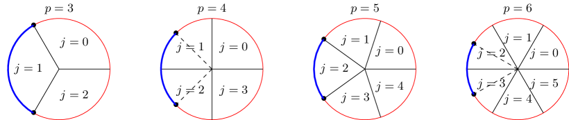
Figure 5: The figure shows how the indices $\boldsymbol{j}=\{j_{1},\dots,j_{2N/p}\}$ must be chosen in order to minimize the $\lambda$’s in Eq. (41). For $\phi_{k}\in(0,2\pi/p)$, the angles $\phi_{k}+2\pi j_{k}/p$ fall into the sectors indicated in the figure depending on the value of $j_{k}$. It is clear that to minimize $\lambda(\phi_{k})$ we should choose $\bar{j}_{k}$ such that $\phi_{k}+2\pi\bar{j}_{k}/p$ belongs to the blue arc $(\pi-\pi/p,\pi+\pi/p)$. In particular, if $p=2m+1$, $\bar{j}_{k}=m$ for any $\phi_{k}$, while if $p=2m$, $\bar{j}_{k}=m-1$ when $\phi_{k}>\pi/p$ and $\bar{j}_{k}=m$ if $\phi_{k}<\pi/p$. There is only one choice of $\boldsymbol{j}$ that realizes the minimum; the blue arc is a Fermi sea for $\arccos(h)=\pi-\pi/p$.

VI Conclusions

In this paper we studied in detail a vast class of ground state overlaps in the XY chain when the number of lattice sites is even ($L=2N$). In particular, we provided an explicit determinant representation, see Eq. (17), adapting to imaginary times the formalism developed in RA for the Return Amplitude. From such a determinant representation we extracted the large $N$ limit by proving a general formula,  see Eq. (47), for the principal minors of circulant matrices. The finite $O(1)$ contribution in the thermodynamic limit of the overlap at criticality is shown to be $\gamma$-independent for all the states considered. Its logarithm defines the universal renormalized Boundary Entropy boundary , which was proven to have only two possible values depending on whether the quantum state flows to the free conformal boundary state or to the linear superposition of fixed conformal boundary states. Linear superpositions of fixed conformal boundary states appear naturally also in the analysis of topological defects GW , as a result of the Kramers-Wannier duality applied to the free boundary state Kon ; chiral ; FI .

As already mentioned, for technical reasons, our analysis has been limited to a chain with an even number of lattice sites and the expressions for the ground state overlaps are valid outside the circle $\gamma^{2}+h^{2}=1$. This is not a strong limitation, since the domain covers almost all the relevant critical cases OYNR . For chains with an odd number of lattice sites and $h<0$ or inside the circle $\gamma^{2}+h^{2}=1$, however, the lowest-energy state might belong to the Ramond sector. In this case, finite-size corrections could develop also subleading logarithmic terms $O(\log N)$ Navot2 . It would be interesting to investigate this possibility and its implications in the future: the existence of logarithmic corrections to the scaling can spoil, for instance, the universality of the $O(1)$ contribution. It is also worth to further test the universality conjecture for the Boundary Entropies at the critical point by considering irrelevant integrability breaking interactions, such as next-to-next neighbour couplings. Overlaps can be calculated numerically through Matrix Product approximations of the ground state.

Finally, we have also discussed the case $\gamma=0$, where Formation Probabilities are directly related to the multiplicity of the ground state Boltzmann weight in the large $\beta$ expansion of a suitable determinant, see Eq. (40). In this case, our study extends considerably the analytic results for the overlaps presented in MS .

Appendix A Euler-MacLaurin (EM) summation formulas

EM Summation Formula.—If $f(x)$ is a differentiable function in the interval $0\leq x\leq 1$, then

$$\sum_{k=1}^{N}f\left(\frac{k-1/2}{N}\right)=N\int_{0}^{1}dxf(x)-\frac{f^{\prime}(1)-f^{\prime}(0)}{24}\left(\frac{1}{N}\right)+O(1/N^{2}),$$ (43)

see Eq. (1) in Navot1 for $a=1/2$. In Navot2 , an extension of the EM summation formula was proven, of which we made extensive application in this paper.

Extended EM Summation Formula.— Take an integrable function $f(x)$, in the interval $0\leq x\leq 1$, such that $f(x)\stackrel{{\scriptstyle x\rightarrow 0}}{{\rightarrow}}\log x^{\alpha}$, $\alpha\in\mathbb{R}$. Then the following summation formula holds

$$\sum_{k=1}^{N}f\left(\frac{k-1/2}{N}\right)=N\int_{0}^{1}dxf(x)+\frac{\alpha\log 2}{2}+O(1/N),$$ (44)

see Eq. (7) in Navot2 for $g(x)=\alpha$ and $a=1/2$. Notice that differently from Eq. (43), the $O(1)$ term is now non-zero. If more than one logarithmic singularity is present on the integration domain, it is always possible to divide it in subsets such that any subset will contain only one singularity. It is clear than that the contributions of different singularities add up.

For the sake of completeness, we provide a quick but non rigorous proof of Eq. (44). Let us consider $f(x)$ as above and rewrite $f(x)=g(x)+\alpha\log(x)$, where $g(x)\equiv f(x)-\alpha\log(x)$ satisfies the hypothesis of the EM Summation Formula, Eq. (43). Proving the extended EM Summation Formula boils down to estimate the large $N$ limit of the sum

$$\sum_{k=1}^{N}\log\left(\frac{k-1/2}{N}\right),$$ (45)

which can be done by expanding its exponential, i.e. $\frac{(2N-1)!!}{(2N)^{N}}$, for $N\gg 1$. By applying the Stirling formula one obtain $\frac{(2N-1)!!}{(2N)^{N}}=\sqrt{2}e^{-N+O(1/N)}$ from which Eq. (44) easily follows Ref2 .

Appendix B Proof of Eq. (23)

In order to determine the overlap in Eq. (17) and especially the determinant of the $(sM)\times(sM)$ matrix $\textbf{W}_{\sigma}$, we proceed as follows. Let us introduce a $2N\times 2N$ diagonal matrix $\textbf{I}^{(sp)}$, with elements $[\textbf{I}^{(sp)}]_{lm}=\delta_{l,m}\delta_{l,q}$, being $q$ the position of an up spin in the configuration labelled by $\mathcal{B}_{s,p}$. The matrix $\textbf{W}^{\prime}_{\sigma}=\textbf{W}\textbf{I}^{(sp)}$ will have rank $sM$ and columns of zeros in correspondence with the positions of the down spins. Consider now the characteristic polynomial

$$\mathfrak{P}_{M}\equiv\det(\lambda\textbf{I}-\textbf{W}_{\sigma}^{\prime})=\sum_{n=0}^{2N}c_{n}\lambda^{n}.$$ (46)

It is known, see for example Matan , that its coefficients $c_{n}$ can be expressed in terms of the principal minors of order $2N-n$ of the matrix $\textbf{W}_{\sigma}^{\prime}$. We recall for convenience that a principal minor of order $2N-n$ of a $2N\times 2N$ matrix is the determinant of the $(2N-n)\times(2N-n)$ sub-matrix obtained by removing the same set of $n$ rows and columns from the original matrix. It then follows from the previous considerations and the definition of the matrix $\textbf{W}_{\sigma}$ in Eq. (17) that the first non-vanishing coefficient of the characteristic polynomial in Eq. (46) is $c_{2N-sM}=c_{M(p-s)}$ and moreover

$$c_{M(p-s)}=\det\textbf{W}_{\sigma}.$$ (47)

We now discuss how the coefficient $c_{M(p-s)}$ of the characteristic polynomial in Eq. (46) can be calculated in closed form.

The matrix $\textbf{I}^{(sp)}$, entering the definition of $\textbf{W}_{\sigma}^{\prime}$, reads (see for instance LC )

$$[\textbf{I}^{(sp)}]_{lm}=\frac{\delta_{lm}}{p}\sum_{j=0}^{p-1}\sum_{r=0}^{s-1}e^{\frac{2\pi ij(l+r)}{p}}.$$ (48)

Notice also that the matrix W is circulant (cf Eq. (15)) and can be diagonalized by the unitary matrix $[\textbf{U}]_{lk}=\frac{1}{\sqrt{2N}}e^{il\phi_{k}}$, in particular $\textbf{D}_{W}\equiv\textbf{U}\textbf{W}\textbf{U}^{\dagger}=\text{diag}(w(\phi_{1}),\dots,w(\phi_{2N}))$. Because of the form of the states chosen in Sec. IV, see Eq. (22), $2N=Mp$. To express the coefficient $c_{M(p-s)}$ of the characteristic polynomial of the matrix $\textbf{W}_{\sigma}^{\prime}$ in terms of the eigenvalues of W, it is convenient to rewrite

$$\mathfrak{P}_{M}(\lambda;\mathcal{W})=\det(\lambda\textbf{I}-\overbrace{\textbf{D}_{W}\textbf{U}\textbf{I}^{(sp)}\textbf{U}^{\dagger}}^{\textbf{A}_{M}}),$$ (49)

where $\mathcal{W}=\{w(\phi_{1}),\dots,w(\phi_{Mp})\}$ and we made evident all the variable dependence. In the rest of the Appendix, we will further use the shorthand notation $w_{l}$ for $w(\phi_{l})$. The matrix $\textbf{A}_{M}$ can be calculated explicitly from its definition in Eq. (49) and one finds

$$[\textbf{A}_{M}]_{lm}=\frac{w_{l}}{p}~{}\delta_{l,m}^{\text{mod}M}\sum_{j=p-s+1}^{p}e^{\frac{2\pi i(j-1/2)(l-m)}{Mp}},$$ (50)

with $l,m=1,\dots,Mp$. However, since $l-m=Mk~{}(k=0,\dots,p-1)$ as a consequence of the Kronecker symbol, Eq. (50) simplifies to

$$[\textbf{A}_{M}]_{lm}=w_{l}~{}\delta_{l,m}^{\text{mod}M}B_{k}\quad\text{where}\quad B_{k}\equiv\frac{1}{p}\sum_{j=p-s+1}^{p}e^{\frac{2\pi i(j-1/2)k}{p}}.$$ (51)

Eq. (51) implies that the coefficients $B_{k}$ are $M$-independent, moreover it is easy to verify that $\textbf{A}_{1}$ coincides with A in Eq. (24), replacing $w_{l}\leftrightarrow x_{l}$. By denoting with $[\bullet]_{\lambda}=\lambda\cdot 1-\bullet$, the characteristic polynomial of $\textbf{A}_{1}$ is

$$\mathfrak{P}_{1}(\lambda;\{w_{1},\dots,w_{p}\})=\det\begin{bmatrix}[w_{1}B_{0}]_{\lambda}&-w_{1}B_{1}&-w_{1}B_{2}&\dots&-w_{1}B_{p-1}\\ -w_{2}B_{1}^{*}&[w_{2}B_{0}]_{\lambda}&-w_{2}B_{1}&\dots&-w_{2}B_{p-2}\\ \vdots&\vdots&\vdots&\vdots&\vdots\\ -w_{p}B_{p-1}^{*}&-w_{p}B_{p-2}^{*}&-w_{p}B_{p-3}^{*}&\dots&[w_{p}B_{0}]_{\lambda}\\ \end{bmatrix}.$$ (52)

To demonstrate Eq. (23) one proceeds by induction on $M$. First, we will prove that the characteristic polynomial of the matrix $\textbf{A}_{M}$ is factorized, that is

$$\mathfrak{P}_{M}(\lambda;\mathcal{W})=\prod_{k=1}^{M}\mathfrak{P}_{1}(\lambda;\mathcal{W}_{k}),$$ (53)

where each of the $M$ sets $\mathcal{W}_{k}$ contain the $p$ variables $w_{k+jM}$ for $j=0,\dots,p-1$.

A moment of thought shows that $\textbf{A}_{M}$ is actually $\textbf{A}_{1}$ with the property that elements on different diagonals have been separated by $M-1$ diagonals of zeros; therefore its characteristic polynomial $\mathfrak{P}_{M}$ is

$$\det\left\lceil\begin{matrix}[w_{1}B_{0}]_{\lambda}&0&\dots&0&-w_{1}B_{1}&0&\dots&0&-w_{1}B_{2}\\ 0&[w_{2}B_{0}]_{\lambda}&0&\dots&0&-w_{2}B_{1}&0&\dots&0\\ \vdots&\vdots&\vdots&\vdots&\vdots&\vdots&\vdots&\vdots&\vdots\\ 0&\dots&0&[w_{M}B_{0}]_{\lambda}&0&\dots&0&-w_{M}B_{1}&0\\ -w_{M+1}B_{1}^{*}&0&\dots&0&[w_{M+1}B_{0}]_{\lambda}&0&\dots&0&-w_{M+1}B_{1}\\ \vdots&\vdots&\vdots&\vdots&\vdots&\vdots&\vdots&\vdots&\vdots\end{matrix}\right..$$ (54)

Ignoring signs that can be easily traced back, it is possible to move columns and rows of the matrix in Eq. (54) to calculate its determinant. We then accommodate to the left, after $\frac{(M-1)p(p-1)}{2}$ exchanges, all the columns that contain the variables $w_{1},w_{1+M},w_{1+2M},\dots,w_{1+(p-1)M}$. Dropping a factor $(-1)^{\frac{(M-1)p(p-1)}{2}}$, one ends up with the following expression for $\mathfrak{P}_{M}$

$$\det\left\lceil\begin{matrix}[w_{1}B_{0}]_{\lambda}&-w_{1}B_{1}&\dots&-w_{1}B_{p-1}&0&0&0&\dots&0\\ 0&0&\dots&0&[w_{2}B_{0}]_{\lambda}&0&\dots&0&-w_{2}B_{1}\\ 0&0&\dots&0&0&[w_{3}B_{0}]_{\lambda}&0&\dots&0\\ \vdots&\vdots&\vdots&\vdots&\vdots&\vdots&\vdots&\vdots&\vdots\\ -w_{M+1}B_{1}^{*}&[w_{M+1}B_{0}]_{\lambda}&\dots&-w_{M+1}B_{p-2}&0&0&0&\dots&0\\ 0&0&\dots&0&-w_{M+2}B_{1}^{*}&0&\dots&0&[w_{M+2}B_{0}]_{\lambda}\\ \vdots&\vdots&\vdots&\vdots&\vdots&\vdots&\vdots&\vdots&\vdots\end{matrix}\right..$$ (55)

By pushing up, with again $\frac{(M-1)p(p-1)}{2}$ exchanges, all the rows labelled by $1+jM$ with $j=1,\dots,p-1$ of Eq. (55), we finally arrive at

$$\mathfrak{P}_{M}=\det\begin{bmatrix}[\textbf{A}_{1}(\mathcal{W}_{1})]_{\lambda}&\textbf{0}\\ \textbf{0}&[\textbf{A}_{M-1}(\overline{\mathcal{W}}_{1})]_{\lambda}\\ \end{bmatrix}.$$ (56)

The notation in Eq. (56) indicates that the matrix $\textbf{A}_{1}$ contains all the variables in the set $\mathcal{W}_{1}=\{w_{1},\dots,w_{M(p-1)+1}\}$ organized in the same order as in Eq. (52).The matrix $\textbf{A}_{M-1}$ is instead a function of the remaining variables; namely $\overline{\mathcal{W}}_{1}=\mathcal{W}\backslash\mathcal{W}_{1}$. We have then proven that

$$\mathfrak{P}_{M}(\lambda;\mathcal{W})=\mathfrak{P}_{1}(\lambda;\mathcal{W}_{1})\mathfrak{P}_{M-1}(\lambda;\overline{\mathcal{W}}_{1}).$$ (57)

By applying the inductive hypothesis to $\mathfrak{P}_{M-1}$ in Eq. (57), the first part of our proof, i.e. Eq. (53), now follows. It is left to show that the coefficient of the lowest power of $\lambda$ in $\mathfrak{P}_{M}(\lambda;\mathcal{W})$ is also factorized. The matrix $\textbf{A}_{1}$ has rank $s$ and $p-s$ among its eigenvalues are zero. Let $\mathcal{P}_{j}(x_{1},\dots,x_{p})$ with $j=0,\dots,s$ denote the coefficients of $\lambda^{p-s+j}$ in the characteristic polynomial $\mathfrak{P}_{1}(\lambda;\{x_{1},\dots,x_{p}\})$. The latter are determined recursively by the Faddeev-Le Verrier algorithm FF ; for example: $\mathcal{P}_{s}=1$ and $\mathcal{P}_{s-1}=-\text{Tr}[\textbf{A}_{1}]$. From Eq. (53) we thus conclude that

$$\mathfrak{P}_{M}(\lambda;\mathcal{W})=\lambda^{M(p-s)}\prod_{k=1}^{M}\left[\mathcal{P}_{s}(w_{k},\dots,w_{k+(p-1)M})\lambda^{s}+\dots+\mathcal{P}_{0}(w_{k},\dots,w_{k+(p-1)M})\right],$$ (58)

where we have made explicit the variable dependence of the polynomials $\mathcal{P}_{j}$. The lowest power of $\lambda$ in Eq. (58) is $M(p-s)$ and its coefficient is

$$c_{M(p-s)}=\prod_{k=1}^{M}\mathcal{P}_{0}(w_{k},\dots,w_{k+(p-1)M}),$$ (59)

eventually proving Eq. (23). Notice that the result in Eq. (59) holds for any circulant matrix W.

Appendix C Additional Examples

In the final Appendix, we gather additional examples of calculations of the BE for states labelled by the blocks $\mathcal{B}_{s,p}$ at $\gamma\not=0$. The results are summarized in Tab. 1, where we provide the polynomial $\mathcal{P}_{0}(x_{1},\dots,x_{p})$, see Eq. (25), and the values of the BE along the critical lines $h=\pm 1$. The latter, as explained in many occasions in the main text, are obtained by analyzing the zeros and singularities in the domain $\phi\in[0,2\pi/p]$ of the function

$$g_{s,p}(\phi)\equiv|\mathcal{P}_{0}\bigl{(}w(\phi),w(\phi+2\pi/p),\dots,w(\phi+2\pi(p-1)/p)\bigr{)}|,$$ (60)

and applying Eq. (44).

$\mathcal{B}_{s,p}$	$\mathcal{P}_{0}(x_{1},\dots,x_{p})$	$s_{\sigma}(1)$	$s_{\sigma}(-1)$
$\mathcal{B}_{2,3}$	$\frac{1}{3}(x_{1}x_{2}+x_{1}x_{3}+x_{2}x_{3})$	$\frac{1}{2}\log 2$	0
$\mathcal{B}_{2,5}$	$\frac{1}{50}\left(x_{1}\left(\eta x_{3}+\eta x_{4}+\xi x_{2}+\xi x_{5}\right)+x_{2}\left(\eta\left(x_{4}+x_{5}\right)+\xi x_{3}\right)+\eta x_{3}x_{5}+\xi x_{4}\left(x_{3}+x_{5}\right)\right)$	$\frac{1}{2}\log 2$	0
$\mathcal{B}_{3,5}$	$\frac{1}{50}\left(x_{2}\left(x_{4}\left(-\eta x_{5}-\xi x_{3}\right)-\eta x_{3}x_{5}\right)+x_{1}\left(x_{2}\left(-\eta x_{4}-\xi x_{3}-\xi x_{5}\right)-\eta x_{3}\left(x_{4}+x_{5}\right)-\xi x_{4}x_{5}\right)-\xi x_{3}x_{4}x_{5}\right)$	0	$\frac{1}{2}\log 2$
$\mathcal{B}_{4,5}$	$\frac{1}{5}\left(x_{2}x_{3}x_{4}x_{5}+x_{1}\left(x_{3}x_{4}x_{5}+x_{2}\left(x_{3}x_{4}+\left(x_{3}+x_{4}\right)x_{5}\right)\right)\right)$	$\frac{1}{2}\log 2$	0

Table 1: Results for the BEs up to $p=5$, $s_{\sigma}=0$ corresponds to the free boundary state, while $s_{\sigma}=\frac{1}{2}\log 2$ indicates renormalization toward the linear superposition of fixed boundary states. In the Table, we have defined $\eta=5+\sqrt{5}$, $\xi=5-\sqrt{5}$. Mathematica gives explicit expressions for the polynomials also for larger values of $p$ but they become increasingly cumbersome. The values of the BEs calculated from Eq. (44) are consistent with the general pattern enunciated at the end of Sec. IV.

References

- (1) V. E. Korepin, A. G. Izergin, F. H. L. Essler and D. B. Uglov, Correlation function of the spin 1/2 XXX antiferromagnet, Phys. Lett. A 190, 182 (1994).
- (2) F. H. L. Essler, H. Frahm, A. G. Izergin and V. E. Korepin, Determinant representation for correlation functions of spin 1/2 XXX and XXZ Heisenberg magnets, Commun. Math. Phys. 174, 191 (1995).
- (3) F. H. L. Essler, H. Frahm, A. R. Its and V. E. Korepin, Integrodifference equation for a correlation function of the spin 1/2 Heisenberg XXZ chain, Nucl. Phys. B 446, 448 (1995).
- (4) M. Shiroishi, M. Takahashi and Y. Nishiyama, Emptiness formation probability for the one-dimensional isotropic XY model, J. Phys. Soc. Jpn. 70, 3535 (2001).
- (5) N. Kitanine, J. M. Maillet, N. A. Slavnov, V. Terras, Emptiness formation probability of the XXZ spin- Heisenberg chain at , J. Phys. A 25, L385 (2002).
- (6) V. E. Korepin, S. Lukyanov, Y. Nishiyama, and M. Shiroishi, Asymptotic behavior of the emptiness formation probability in the critical phase of /XXZ spin chain, Phys. Lett. A 312, 21 (2003).
- (7) F. Franchini and A. Abanov, Asymptotics of Toeplitz determinants and the emptiness formation probability for the XY spin chain, J. Phys. A: Math. Gen. 38 (2005) 5069-5095.
- (8) F. Ares and J. Viti, Emptiness formation probability and the Painlevé V equation in the XY spin chian, J. Stat. Mech. (2020) 013105.
- (9) J-M Stéphan, Emptiness formation probability, Toeplitz determinants, and conformal field theory, J. Stat. Mech. (2013) 05010.
- (10) M. A. Rajabpour, Formation probabilities in quantum critical chains and Casimir effect, EPL 122, 66001 (2015).
- (11) M. A. Rajabpour, Finite size corrections to scaling of the formation probabilities and the Casimir effect in the conformal field theories, J. Stat. Mech. (2016) 123101.
- (12) N. Allegra, J. Dubail, J-M. Stéphan, and J. Viti, Inhomogeneous field theory inside the arctic circle J. Stat. Mech. (2016) 053108.
- (13) K. Najafi and M. A. Rajabpour, Formation probabilities and Shannon information and their time evolution after quantum quench in the transverse-field XY chain, Phys. Rev. B 93, 125139 (2016).
- (14) M. N. Najafi and M. A. Rajabpour, Formation probabilities and statistics of observables as defect problems in the free fermions and the quantum spin chains, Phys. Rev. B 101, 165415 (2020).
- (15) I. Affleck and A. Ludwig, Universal noninteger “ground-state degeneracy”in critical quantum systems, Phys. Rev. Lett. 67, 161 (1991).
- (16) A. LeClair, G. Mussardo, H. Saleur, and S. Skorik, Boundary energy and boundary states in integrable quantum field theories, Nucl. Phys.B453(1995) 581–618
- (17) P. Dorey, A. Pocklington, R. Tateo, and G. Watts, TBA and TCSA with boundaries andexcited states, Nucl. Phys.B525(1998) 641–663.
- (18) P. Dorey, I. Runkel, R. Tateo, and G. Watts, -functionflow in perturbed boundaryconformal field theories, Nucl. Phys.B578(2000) 85–122
- (19) D. Friedan and A. Konechny, On the boundary entropy of one-dimensional quantumsystems at low temperature, Phys. Rev. Lett.93(2004) 030402
- (20) P. Dorey, D. Fioravanti, C. Rim, and R. Tateo, Integrable quantum field theory withboundaries: The exact g-function, Nucl. Phys.B696(2004) 445–467
- (21) B. Pozsgay, On O(1) contributions to the free energy in Bethe Ansatz systems: The Exact g-function, JHEP08(2010) 090
- (22) J. Caetano, S. Komatsu, Functional Equations and Separation of Variablesfor Exact -Function, [arXiv:2004.05071]
- (23) J. Cardy, Bulk Renormalization Group Flows and Boundary States in Conformal Field Theories, SciPost 3, 011 (2017).
- (24) T.-C. Wei, D. Das, S. Mukhopadyay, S. Vishveshwara and P. Goldbart, Global entanglement and quantum criticality in spin chains Phys. Rev. A71, 060305 (2005)
- (25) J-M. Stéphan, S. Furukawa, G. Misguich, and V. Pasquier, Shannon and entanglement entropies of one- and two-dimensional critical wave functions Physical Review B 80, 184421 (2009)
- (26) Ching-Yu Huang and Feng-Li Lin, Multipartite entanglement measures and quantum criticality from matrix and tensor product states Phys. Rev. A81,032304 (2010)
- (27) J-M. Stéphan, G. Misguich, and V. Pasquier, Rényi entropy of a line in two-dimensional Ising model Phys. Rev. B 82, 125455 (2010)
- (28) Qian-Qian Shi and Román Orús and John Ove Fjærestad and Huan-Qiang Zhou, Finite-size geometric entanglement from tensor network algorithms, New Journal of Physics12, 025008 (2010)
- (29) J-M. Stéphan, G. Misguich, and F. Alet, Geometric entanglement of critical XXZ and Ising chains and Affleck-Ludwig boundary entropies, Phys. Rev. B 82, 180406(R) (2010)
- (30) M. Brockmann and J-M. Stéphan Universal terms in the overlap of the ground state of the spin-1/2 XXZ chain with the Néel state , J. Phys. A: Math. Theor. 50, 354001 (2017).
- (31) J. I. Cirac and G. Sierra, Infinite matrix product states, Conformal Field Theory and the Haldane-Shastry model, , Phys. Rev. B 81, 104431 (2010).
- (32) H. Barnum and N. Linden, Monotones and invariants for multi-particle quantum states J. Phys. A: Math. Gen.34,6787 (2001)
- (33) T.-C. Wei and P. M. Goldbart, Geometric measure of entanglement and applications to bipartite and multipartite quantum states Phys. Rev. A68, 042307(2003).
- (34) P. Calabrese and J. Cardy, Quantum Quenches in Extended Systems, J.Stat.Mech.0706:P06008,2007 (2007).
- (35) I. Navot, An extension of the Euler-MacLaurin summation formula, J. Math. and Phys. 40, 271-276 (1961).
- (36) I. Navot, A further extension of the Euler-MacLaurin summation formula, J. Math. and Phys. 41, 155-163 (1962).
- (37) E. Lieb, T. Schultz and D. Mattis, Two soluble models of an antiferromagnetic chain, Ann. Phys. 16 3 (1961).
- (38) S. Katsura, Statistical Mechanics of the Anisotropic Linear Heisenberg Model, Phys. Rev. 127, 1508 (1962).
- (39) B. Damski and M. Rams, Exact results for fidelity susceptibility of the quantum Ising model: The interplay between parity, system size and magnetic field, J. Phys. A 47, 025303 (2014).
- (40) M. Okuyama, Y. Yamanaka, H. Nishimori and M. Rams, Anomalous behavior of the energy gap in the one-dimensional quantum XY model, Phys. Rev. E 92, 052116 (2015).
- (41) K. Najafi, M. A. Rajabpour and J. Viti, Return amplitude after a quantum quench in the XY chain, J. Stat. Mech. (2019) 083102.
- (42) We thank an anonymous referee for pointing out this potential subtlety.
- (43) H. Blöte, J. Cardy and M. Nightingale, Conformal invariance, the central charge, and universal finite-size amplitudes at criticality, Phys. Rev. Lett. 56, 742 (1986)
- (44) I. Affleck, Universal term in the free energy at a critical point and the conformal anomaly, Phys. Rev. Lett. 56, 746 (1986).
- (45) J. Cardy, Boundary conditions, fusion rules and the Verlinde formula, Nucl. Phys. B 324 3 (1989).
- (46) J. Cardy, Boundary Conformal Field Theory, arXiv: hep-th/0411189.
- (47) A. Konechny, RG boundaries and interfaces in Ising field theory, J.Phys. A50 (2017) no.14, 145403 (2017).
- (48) L. Chim, Boundary S matrix for the tricritical Ising model, J. Mod. Phys. A 11, 4491 (1996).
- (49) I. Affleck, Edge Critical Behaviour of the 2-Dimensional Tri-critical Ising Model, J.Phys.A33:6473-6480 (2000).
- (50) K. Graham, I. Runkel and G.M.T. Watts, Renormalization group flows of boundary theories, arXiv: hep-th/0010082 (2000).
- (51) K. Graham and G.M.T. Watts, Defect lines and boundary flows, JHEP 2004 (4), 019 (2004).
- (52) A. Konechny, Open topological defects and boundary RG flows, arXiv: 1911.06041 (2019).
- (53) Y. Fukusumi and S. Iino, Open spin chain realization of topological defect on 1d Ising model and boundary bulk symmetry, arXiv: 2004.04415 (2020).
- (54) K. Najafi, M. A. Rajabpour and J. Viti, Light-cone velocities after a global quench in a non-interacting model, Phys. Rev. B 97, 205103 (2018).
- (55) M. Lencsés, J. Viti and G. Takács, Chiral Entanglement in massive quantum field theories in 1+1 dimensions, JHEP 2019 (1), 177 (2019).
- (56) M. Oshikawa, I. Affleck, Boundary conformal field theory approach to the two-dimensional critical Ising model with a defect line, 10.1016/S0550-3213(97)00219-8
- (57) D. Radicevic, Spin Structures and Exact Dualities in Low Dimensions, arXiv:1809.07757 (2018) .
- (58) P. Mazza, J-M. Stéphan, E. Canovi, V. Alba, M. Brockmann and M. Haque, Overlap distributions for quantum quenches in the anisotropic Heisenberg chain, J. Stat. Mech. (2016) P013104.
- (59) We are grateful to an anonymous referee for suggesting this line of proof.
- (60) R. Horn, C. Johnson, Matrix Analysis, CUP, New York (2013).
- (61) D. Faddeev and V. Faddeeva, Computational methods of linear algebra, J. Math. Sci. 15, 531–650 (1981).