A survey on sufficient optimality conditions for delayed optimal control problems

Abstract

The aim of this work is to make a survey on recent sufficient optimality conditions for optimal control problems with time delays in both state and control variables. The results are obtained by transforming delayed optimal control problems into equivalent non-delayed problems. Such approach allows to use standard theorems that ensure sufficient optimality conditions for non-delayed optimal control problems. Examples are given with the purpose to illustrate the results.

1. Introduction

The study of delayed systems, which can be optimized and controlled by a certain control function, has a long history and has been developed by many researchers (see, e.g., [2, 3, 6, 9, 17, 22, 26, 29, 54, 69] and references cited therein). Such systems can be called retarded, time-lag, or hereditary processes/optimal control problems. There are many applications of such systems, in diverse fields as Biology, Chemistry, Mechanics, Economy and Engineering (see, e.g., [3, 17, 27, 37, 41, 64, 69, 70, 71]). Dynamical systems with time delays, in both state and control variables, play an important role in the modelling of real-life phenomena, in various fields of applications (see [26, 27]). For instance, in [60] the incubation and pharmacological delays are modelled through the introduction of time delays in both state and control variables. In [67], Silva et al. introduce time delays in the state and control variables for tuberculosis modelling. They represent the time delay on the diagnosis and commencement of treatment of individuals with active tuberculosis infection and the delays on the treatment of persistent latent individuals, due to clinical and patient reasons.

Delayed linear differential systems have also been investigated, their importance being recognized both from a theoretical and practical points of view. For instance, in [22], Friedman considers linear hereditary processes and apply to them Pontryagin’s method, deriving necessary optimality conditions as well as existence and uniqueness results. Analogously, in [54], delayed linear differential equations and optimal control problems involving this kind of systems are studied. Since these first works, many researchers have devoted their attention to linear quadratic optimal control problems with time delays (see, e.g., [9, 16, 18, 40, 55]). It turns out that for delayed linear quadratic optimal control problems it is possible to provide an explicit formula for the optimal controls (see [9, 40, 55]).

Delayed optimal control problems with differential systems, which are linear both in state and control variables, have been studied in [9, 13, 16, 18, 40, 42, 43, 46, 53, 55]. In [16, 42, 55], the system is delayed with respect to state and control variables. In [13, 53], the system only considers delays in the state variable. Chyung and Lee derive necessary and sufficient optimality conditions in [13], while Oğuztöreli only proves necessary conditions in [53]. Certain necessary conditions analysed by Chyung and Lee in [13] have been already derived in [30, 58, 59]. However, the system considered in [13] is different from the previously studied hereditary systems, which do not require a initial function of state. In [18], Eller et al. derive a sufficient condition for a control to be optimal for certain problems with time delay. The problems studied by Eller et al. and Khellat in [18] and [40], respectively, consider only one constant lag in the state. The research done by Lee in [46] is different from that of the current work (more specifically from that of Section 3), because in [46] the aim is to minimize a cost functional, which does not consider delays, subject to a linear differential system (with respect to state and control variables) and to another constraint. In their differential system, the state variable depends on a constant and a fixed delay, while the control variable depends on a constant lag, which is not specified a priori. Note that the differential system of the problem considered in [43] is similar to the one of [46]. Although Banks has studied delayed non-linear problems without lags in the control, he has also analysed problems that are linear and delayed with respect to control (see [2]). Later, in 2010, Carlier and Tahraoui investigated optimal control problems with a unique delay in the state (see [10]). In 2012 and 2013, Frederico and Torres devoted their attention to optimal control problems that only contain delays in the state variables and the dependence on the control is linear (see [20, 21]). Recently, Cacace et al. studied optimal control problems that involve linear differential systems with variable delays only in the control (see [9]).

The problems analysed in the current work are different from those considered in the mentioned papers. In Section 3, the optimal control problems involve differential systems that are linear with respect to state, but not with respect to the control. In Section 4, we study optimal control problems with non-linear differential systems. Furthermore, in both Sections 3 and 4, we consider a constant time delay in the state and another one in the control. These two delays are, in general, not equal.

In [35], Hughes firstly consider variational problems with only one constant lag and derive various necessary and a sufficient optimality conditions for them. The variational problems in [35] can easily be transformed into control problems with only one constant delay (see, e.g., [49, p. 53–54]). Hughes also investigates an optimality condition for a control problem with a constant delay, which is the same for state and control. The problems analysed by Chan and Yung in [11], and by Sabbagh in [62], are similar to the first problems studied by Hughes in [35]. Therefore, the problems investigated in [11, 35, 62] are different from the problems studied by us here, because in the present work the state delay is not necessarily equal to the control delay. The problems considered in [35, 62] are also considered in [56] by Palm and Schmitendorf. For such problems, they derive two conjugate-point conditions, which are not equivalent. Note that their conditions are only necessary and do not give a set of sufficient conditions (see [56]). Recent results include Noether type theorems for problems of the calculus of variations with time delays (see [19, 52, 65]), necessary optimality conditions for quantum (see [21]) and Herglotz variational problems with time delays (see [63, 64]), as well as delayed optimal control problems with integer (see [5, 8, 20]) and non-integer (fractional order) dynamics (see [14, 15]). Applications of such theoretical results are found in Biology and other Natural Sciences, e.g., in tuberculosis (see [67]) and HIV (see [60, 61]).

In [39], Jacobs and Kao investigate delayed problems that consist to minimize a cost functional without delays subject to a differential system defined by a non-linear function with a delay in state and another one in the control. Similarly to our problems, these delays do not have to be equal. In contrast, all types of cost functionals considered in our work also contain time delays. Therefore, we study here problems that are more general than the one considered in [39]. Jacobs and Kao transform the problem using a Lagrange-multiplier technique and prove a regularity result in the form of a controllability condition, as well as some necessary optimality conditions. Then, in some special restricted cases, they prove existence, uniqueness, and sufficient conditions. Such restricted problems consider a differential system that is linear in state and in control variables. Thus, the sufficient conditions of [39] are derived for problems that are less general than ours.

As it is well-known, and as Hwang and Bien write in [36], many researchers have directed their efforts to seek sufficient optimality conditions for control problems with delays (see, e.g., [13, 18, 35, 39, 48, 66]). Therefore, it is not a surprise that there are authors that already proved some sufficient optimality conditions for delayed optimal control problems similar but, nevertheless, different from ours. In what respects to research done in [13, 18, 35, 39], we have already seen why they are different. The delayed optimal control problems analysed by Schmitendorf in [66] have a cost functional and a differential system that are more general than ours. However, in [66] the control takes its values in all $\mathbb{R}^{m}$, while in the present work the control values belong to a set $U\subseteq\mathbb{R}^{m}$, $m\in\mathbb{N}$. In [48], Lee and Yung study a problem that is similar to the one considered in [66], where the control belongs to a subset of $\mathbb{R}^{m}$, as we consider here. First and second-order sufficient conditions are shown in [48]. Nevertheless, the conditions of [48] are not constructive and not practical for the computation of the optimal solution. Indeed, as hypothesis, it is assumed the existence of a symmetric matrix under some conditions, for which is not given a method to calculate its expression. Another similar problem to ours is studied by Bokov in [8], in order to arise a necessary optimality condition in an explicit form. Moreover, a solution to the problem with infinite time horizon is given in [8]. In contrast, in the present work we are interested to derive sufficient optimality conditions. In [36], Hwang and Bien prove a sufficient condition for problems involving a differential affine time delay system with the same time delay for the state and the control. The differential systems considered in the present work are more general. In 1996, Lee and Yung, considering functions that do not have to be convex, derived various first and second-order sufficient conditions for non-linear optimal control problems with only a constant delay in the state (see [45]). Their class of problems is obviously different from our. In particular, we consider delays for both state and control variables. As in [11, 48], second-order sufficient conditions are shown to be related to the existence of solutions of a Riccati-type matrix differential inequality.

Optimal control problems with multiple delays have also been investigated. In [29], Halanay derive necessary conditions for some optimal control problems with various time lags in state and control variables, using the abstract multiplier rule of Hestenes (see [34]). In [29], all delays related to state are equal to each other and the same happens with the delays associated to the control. Note that the results of [22, 30] are obtained as particular cases of problems considered in [29]. Later, in 1973, a necessary condition is derived for an optimal control problem that involves multiple constant lags only in the control. This delayed dependence occurs both in the cost functional and in the differential system, which is defined by a non-linear function (see [68]). In [32], Haratišvili and Tadumadze prove the existence of an optimal solution and a necessary condition for optimal control systems with multiple variable time lags in the state and multiple variable commensurable time delays in the control. Later, an optimal control problem where the state variable is solution of an integral equation with multiple delays, both on state and control variables, is studied by Bakke in [1]. Furthermore, necessary conditions and Hamilton–Jacobi equations are derived. In 2006, Basin and Rodriguez-Gonzalez proved a necessary and a sufficient optimality condition for a problem that consists to minimize a quadratic cost functional subject to a linear system with multiple time delays in the control variable (see [4]). In their work, they begin by deriving a necessary condition through Pontryagin’s Maximum Principle. Afterwards, sufficiency is proved by verifying if the candidate found, through the Maximum Principle, satisfies the Hamilton–Jacobi–Bellman equation. Although Basin and Rodriguez-Gonzalez consider multiple time delays, the dependence of the state and control in the differential system is linear. In our current work, the dependence of the control, in the differential systems, is, in general, non-linear. In 2013, Boccia et al. derived necessary conditions for a free end-time optimal control problem subject to a non-linear differential system with multiple delays in the state (see [6]). The control variable is not influenced by time lags in [6]. Recently, in 2017, Boccia and Vinter obtained necessary conditions for a fixed end-time problem with a constant and unique delay for all variables, as well as free end-time problems without control delays (see [7]).

As Guinn wrote in [28], the classical methods of obtaining necessary conditions for retarded optimal control problems (used, for instance, by Halanay in [29], Haratišvili in [31] and Oǧuztöreli in [54]) require complicated and extensive proofs (see, e.g., [2, 22, 29, 31, 54]). In $1976$, Guinn proposed a method whereby we can reduce some specific time-lag optimal control problems to equivalent and augmented optimal control problems without delays (see [28]). By reducing delayed optimal control problems into non-delayed ones, we can then use well-known theorems, applicable for optimal control problems without delays, to derive desired optimality conditions for delayed problems (see [28]). In [28], Guinn study specific optimal control problems with a constant delay in state and control variables. These two delays are equal. Later, in $2009$, Göllmann et al. studied optimal control problems with a constant delay in state and control variables subject to mixed control-state inequality constraints (see [26]). In that research, the delays do not have to be equal. For technical reasons, the authors need to assume that the ratio between these two time delays is a rational number (see [26]). In [26], the method used by Guinn in [28] is generalized and, consequently, a non-delayed optimal control problem is again obtained. Pontryagin’s Minimum Principle, for non-delayed control problems with mixed state-control constraints, is used and first-order necessary optimality conditions are derived for retarded problems (see [26]). Furthermore, Göllmann et al. discuss the Euler discretization of the retarded problem and some analytical examples versus correspondent numerical solutions are given. For more on numerical methods, for solving applied optimal control problems of systems governed by delay differential equations, see [12, 33, 38]. Later, in 2014, Göllmann and Maurer generalized the research mentioned before, by studying optimal control problems with multiple and constant time delays in state and control, involving mixed state-control inequality constraints (see [27]). Again, necessary optimality conditions are derived (see [27]). Note that the works [26, 27, 28, 29] consider delayed non-linear differential systems.

In Section 3, we consider optimal control problems that consist to minimize a delayed non-linear cost functional subject to a delayed differential system that is linear with respect to state, but not with respect to control. Note that the cost functional does not have to be quadratic, but it satisfies some continuity and convexity assumptions. In Section 4, we consider optimal control problems that consist to minimize a delayed non-linear cost functional subject to a delayed non-linear differential system. In both Sections 3 and 4, the delay in the state is the same for the cost functional and for the differential system. The same happens with the time lag of the control variable. Analogously to Göllmann et al. in [26], we ensure the Commensurability Assumption between the, possibly different, delays of state and control variables. The proofs of our sufficient optimality conditions consider the technique proposed by Guinn in [28] and used by Göllmann et al. in [26, 27] (see [50, 51]). As we have already mentioned before, the technique consists to transform a delayed optimal control problem into an equivalent non-delayed optimal control problem. After doing such transformation, one can apply well-known results for non-delayed optimal control problems and then return to the initial delayed problem. Here we restrict ourselves to delayed problems with deterministic controls. For the stochastic case, we refer the reader to [19, 23, 25, 37, 44].

This work is organised as follows. We begin by recalling the Commensurability Assumption, introduced by Göllmann et al. in [26], and by defining some needed notations, in Section 2. In Section 3.1, we define a state-linear optimal control problem with constant time delays in state and control variables. Then, in Section 3.2, we present a sufficient optimality condition associated with the problem stated in Section 3.1. A concrete example is solved in detail in Section 3.3, with the purpose to illustrate Theorem 3.3 of Section 3.2. In Section 4.2, we present a sufficient optimality condition associated with the non-linear optimal control problem with time lags both in state and control variables, defined in Section 4.1. An example that illustrates the obtained theoretical result – Theorem 4.3 of Section 4.2 – is given. We end with some conclusions, in Section 5.

2. Commensurability assumption and notations

In this section, we recall the Commensurability Assumption introduced by Göllmann et al. in [26].

Assumption 2.1 (See Assumption 4.1 of [26]).

We consider $r,s\geq 0$, not simultaneously equal to zero, and commensurable, that is,

$$(r,s)\neq(0,0)$$

and

$$\frac{r}{s}\in\mathbb{Q}\ \text{ for }\ s>0\ \text{ or }\ \frac{s}{r}\in\mathbb{Q}\ \text{ for }\ r>0.$$

Actually, Commensurability Assumption 2.1 holds for any couple of rational numbers $(r,s)$ for which at least one number is non-zero (see [26]).

With the purpose to simplify the writing, we introduce some notations.

Notation 2.2.

We define $t_{\tau}$, $t^{\tau}$ and $t_{\tau_{1}}^{\tau_{2}}$ as follows:

$$t_{\tau}=t-\tau,\quad t^{\tau}=t+\tau\quad\text{and}\quad t^{\tau_{2}}_{\tau_{1}}=t-\tau_{1}+\tau_{2}$$

for time delays $\tau,\tau_{1},\tau_{2}\in\{r,s\}$ and for all $t\in[a,b]$.

Notation 2.3.

Let $x_{a}=x(a)=\varphi(a)$ and $x_{r}(t)=\big{(}x(t),x(t-r)\big{)}$. Moreover, we define the operators $[\cdot,\cdot]_{r}$ and $\langle\cdot,\cdot\rangle_{r}$ by $[x,\zeta]_{r}(t):=\Big{(}t,x_{r}(t),\zeta\big{(}t,x_{r}(t)\big{)}\Big{)}$ and $\langle x,\zeta\rangle_{r}(t):=\Big{(}t,x_{r}(t),\zeta\big{(}t,x(t)\big{)}\Big{)}$, respectively.

While Notation 2.2 is used in Sections 3 and 4, Notation 2.3 is only considered in Section 4.

3. Delayed state-linear optimal control problem

This section is devoted to state-linear optimal control problems with constant time delays in state and control variables. We make a survey on a sufficient optimality condition for this type of problems. Its proof, and more details associated with the contents of the current section, can be found in [50]. To finish this section, an illustrative example is given.

3.1. Statement of the optimal control problem

We start by defining a delayed state-linear optimal control problem.

Definition 3.1.

Consider that $r\geq 0$ and $s\geq 0$ are constant time delays associated with the state and control variables, respectively. We assume that $(r,s)\neq(0,0)$. A non-autonomous state-linear optimal control problem (OCP${}_{\text{LD}}$) with time delays and with a fixed initial state, on a fixed finite time interval $[a,b]$, consists in

$$\min\ \ C_{LD}\big{(}x(\cdot),u(\cdot)\big{)}=\int_{a}^{b}f^{0}_{x}\big{(}t,x(t),x(t-r)\big{)}+f^{0}_{u}\big{(}t,u(t),u(t-s)\big{)}dt$$

subject to the delayed differential system

$$\dot{x}(t)=A(t)x(t)+A_{D}(t)x(t-r)+g\big{(}t,u(t)\big{)}+g_{D}\big{(}t,u(t-s)\big{)}$$ (3.1)

with the following initial conditions:

$$\begin{split}x(t)&=\varphi(t),\ t\in[a-r,a],\\ u(t)&=\psi(t),\ t\in[a-s,a[,\end{split}$$ (3.2)

where

1. the state trajectory is $x(t)\in\mathbb{R}^{n}$ for each $t\in[a-r,b]$;

2. the control is $u(t)\in U\subseteq\mathbb{R}^{m}$ for each $t\in[a-s,b]$;

3. $A(t)$ and $A_{D}(t)$ are real $n\times n$ matrices for each $t\in[a,b]$.

Next we define admissible pair for (OCP${}_{\text{LD}}$).

Definition 3.2.

We say that $\big{(}x(\cdot),u(\cdot)\big{)}$ is an admissible pair for (OCP${}_{\text{LD}}$) if it respects the following conditions:

1. $\big{(}x(\cdot),u(\cdot)\big{)}\in W^{1,\infty}([a-r,b],\mathbb{R}^{n})\times L^{\infty}([a-s,b],\mathbb{R}^{m})$, where $W^{1,\infty}$ is the space of Lipschitz functions;

2. $\big{(}x(\cdot),u(\cdot)\big{)}$ satisfies the conditions (3.1) and (3.2);

3. $\big{(}x(t),u(t)\big{)}\in\mathbb{R}^{n}\times U$ for all $t\in[a,b]$.

3.2. Main result

In what follows, we consider that the time delays $r$ and $s$ respect the Commensurability Assumption 2.1 and we use Notation 2.2.

The following theorem supplies a sufficient optimality condition associated with (OCP${}_{\text{LD}}$) (see Definition 3.1). Such result generalizes Theorem 5 in Chapter 5.2 of [47].

Theorem 3.3.

Consider (OCP${}_{\text{LD}}$) and assume that

1. functions $f^{0}_{x}$, $\partial_{2}f^{0}_{x}$, $\partial_{3}f^{0}_{x}$, $f^{0}_{u}$, $g$, $g_{D}$, $A$ and $A_{D}$ are continuous for all their arguments;

2. $f^{0}_{x}(t,x,x_{r})$ is a convex function in $(x,x_{r})\in\mathbb{R}^{2n}$ for each $t\in[a,b]$;

3. for almost all $t\in[a,b]$, $u^{*}$ is a control with response $x^{*}$ that satisfies the maximality condition

   $$\begin{split}&\ \max_{u\in U}\big{\{}H_{D}^{1}\big{(}t,x^{*}(t),x^{*}(t_{r}),u,u^{*}(t_{s}),\eta(t)\big{)}\\ &\ +H_{D}^{0}\big{(}t^{s},x^{*}(t^{s}),x^{*}(t^{s}_{r}),u^{*}(t^{s}),u,\eta(t^{s})\big{)}\chi_{[a,b-s]}(t)\big{\}}\\ =&\ H_{D}^{1}\big{(}t,x^{*}(t),x^{*}(t_{r}),u^{*}(t),u^{*}(t_{s}),\eta(t)\big{)}\\ &\ +H_{D}^{0}\big{(}t^{s},x^{*}(t^{s}),x^{*}(t^{s}_{r}),u^{*}(t^{s}),u^{*}(t),\eta(t^{s})\big{)}\chi_{[a,b-s]}(t),\end{split}$$

   where

   $$\begin{split}H_{D}^{p}(t,x,y,u,v,\eta)=&-\Big{[}f^{0}_{x}(t,x,y)+f^{0}_{u}(t,u,v)\Big{]}\\ &+\eta\Big{[}A(t)x+A_{D}(t)y+pg(t,u)+(1-p)g_{D}(t,v)\Big{]}\end{split}$$

   for $p\in\{0,1\}$ and $\eta(t)$ is any non-trivial solution of the adjoint system

   $$\begin{split}\dot{\eta}(t)=&\ \partial_{2}f^{0}_{x}\big{(}t,x^{*}(t),x^{*}(t_{r})\big{)}+\partial_{3}f^{0}_{x}\big{(}t^{r},x^{*}(t^{r}),x^{*}(t)\big{)}\chi_{[a,b-r]}(t)\\ &-\eta(t)A(t)-\eta(t^{r})A_{D}(t^{r})\chi_{[a,b-r]}(t)\end{split}$$

   that satisfies the transversality condition $\eta(b)=[\begin{matrix}0&\cdots&0\end{matrix}]_{1\times n}$.

Then, $\big{(}x^{*}(\cdot),u^{*}(\cdot)\big{)}$ is an optimal solution of (OCP${}_{\text{LD}}$) that leads to the minimal cost $C_{LD}\big{(}x^{*}(\cdot),u^{*}(\cdot)\big{)}$.

The detailed proof of Theorem 3.3 can be found in [50].

3.3. An illustrative example

In this section we provide an illustrative example associated with Theorem 3.3.

Let us consider the delayed state-linear optimal control problem given by

$$\begin{split}\min\ \ \ &C_{LD}\big{(}x(\cdot),u(\cdot)\big{)}=\int_{0}^{4}x(t)+100u^{2}(t)dt\\ \text{s.t.}\ \ &\dot{x}(t)=x(t)+x(t-2)-10u(t-1),\\ &x(t)=1,\ t\in[-2,0],\\ &u(t)=0,\ t\in[-1,0[,\end{split}$$ (3.3)

where $u(t)\in U=\mathbb{R}$ for each $t\in[-1,4]$. Thus, we have that $n=m=1$, $a=0$, $b=4$, $r=2$, $s=1$, $f^{0}_{x}\big{(}t,x(t),x(t-2)\big{)}=x(t)$, $f^{0}_{u}\big{(}t,u(t),u(t-1)\big{)}=100u^{2}(t)$, $A(t)=A_{D}(t)=1$, $g\big{(}t,u(t)\big{)}=0$ and $g_{D}\big{(}t,u(t-1)\big{)}=-10u(t-1)$. Note that our functions respect hypothesis $i$ and $ii$ of Theorem 3.3. Let $\bar{u}$ be an admissible control of problem (3.3) and let us maximize function

$$\begin{split}&-f^{0}_{u}\big{(}t,u,\bar{u}(t-1)\big{)}+\eta(t)g(t,u)\\ &+\big{[}-f^{0}_{u}\big{(}t+1,\bar{u}(t+1),u\big{)}+\eta(t+1)g_{D}(t+1,u)\big{]}\chi_{[0,3]}(t)\\ =&-100u^{2}+\big{[}-100\bar{u}^{2}(t+1)-10\eta(t+1)u\big{]}\chi_{[0,3]}(t)\\ =&\begin{cases}-100u^{2}-10\eta(t+1)u-100\bar{u}^{2}(t+1),\ &t\in[0,3]\\ -100u^{2},\ &t\in\ ]3,4]\end{cases}\end{split}$$

with respect to $u\in\mathbb{R}$. We obtain

$$u(t)=-\frac{\eta(t+1)}{20}$$

for $t\in[0,3]$ and $u(t)=0$ for $t\in\ ]3,4]$. Furthermore, we know that $\eta(t)$ is any non-trivial solution of

$$\begin{split}\dot{\eta}(t)=&\ \partial_{2}f^{0}\big{(}t,x(t),x(t-2)\big{)}+\partial_{3}f^{0}\big{(}t+2,x(t+2),x(t)\big{)}\chi_{[0,2]}(t)\\ &-\eta(t)A(t)-\eta(t+2)A_{D}(t+2)\chi_{[0,2]}(t)\\ \Leftrightarrow\dot{\eta}(t)=&\ 1-\eta(t)-\eta(t+2)\chi_{[0,2]}(t)=\begin{cases}1-\eta(t)-\eta(t+2),\ &t\in[0,2]\\ 1-\eta(t),\ &t\in\ ]2,4]\end{cases}\end{split}$$

that satisfies the transversality condition $\eta(4)=0$. The adjoint system is given by

$$\begin{split}\begin{cases}\dot{\eta}(t)=\begin{cases}1-\eta(t)-\eta(t+2),\ &t\in[0,2]\\ 1-\eta(t),\ &t\in\ ]2,4]\\ \end{cases}\\ \eta(4)=0.\end{cases}\end{split}$$ (3.4)

For $t\in\ ]2,4]$, the solution of differential equation

$$\begin{cases}\dot{\eta}(t)=1-\eta(t)\\ \eta(4)=0\end{cases}$$

is given by $\eta(t)=1-e^{4-t}$. Knowing $\eta(t)$, $t\in\ ]2,4]$, and attending to the continuity of function $\eta$ for all $t\in[0,4]$, we can determine $\eta(t)$ for $t\in[0,2]$ solving the differential equation

$$\begin{cases}\dot{\eta}(t)=1-\eta(t)-\eta(t+2)\\ \eta(2)=1-e^{4-2}=1-e^{2}\end{cases}$$

for $t\in[0,2]$. Therefore, we have that $\eta(t)=e^{2-t}\left(t-e^{2}-1\right)$ for $t\in[0,2]$. Consequently, the solution of the adjoint system (3.4) is given by

$$\begin{split}\eta(t)=\begin{cases}e^{2-t}\left(t-e^{2}-1\right),\ &t\in[0,2]\\ 1-e^{4-t},\ &t\in\ ]2,4].\end{cases}\end{split}$$

So, the control is given by

$$\begin{split}u(t)=\frac{1}{20}\begin{cases}0,\ &t\in[-1,0[\\ e^{3-t}-e^{1-t}t,\ &t\in[0,1[\\ e^{3-t}-1,\ &t\in[1,3]\\ 0,\ &t\in\ ]3,4].\end{cases}\end{split}$$ (3.5)

Knowing the control, we can determine the state by solving the differential equation

$$\begin{cases}\dot{x}(t)=x(t)+x(t-2)-10u(t-1)\\ x(t)=1,\ t\in[-2,0].\end{cases}$$

The state solution is given by

$$\small x(t)=\begin{cases}1,&t\in[-2,0]\\[7.20003pt] -1+2e^{t},&t\in\ ]0,1]\\[7.20003pt] \displaystyle\frac{\left(e^{2}+2e^{4}-2e^{2}t\right)e^{-t}-8+\left(17-2e^{2}\right)e^{t}}{8},&t\in\ ]1,2]\\[7.20003pt] \displaystyle\frac{2e^{4-t}+4+\left(-47e^{-2}+17-2e^{2}+16e^{-2}t\right)e^{t}}{8},&t\in\ ]2,3]\\[7.20003pt] \displaystyle\frac{\left(-e^{6}+e^{4}t\right)e^{-t}+4+\left(-51e^{-2}+24-2e^{2}+17e^{-2}t-2t\right)e^{t}}{8},&t\in\ ]3,4].\end{cases}$$ (3.6)

Such analytical expressions can be obtained with the help of a modern computer algebra system. We have used Mathematica. In Figure 1, we observe that the numerical solutions for control and state, obtained using AMPL [24] and IPOPT [57], are in agreement with their analytical solutions, given by (3.5) and (3.6), respectively. The numerical solutions were obtained using Euler’s forward difference method in AMPL and IPOPT, dividing the interval of time $[0,4]$ into 2000 subintervals. The minimal cost is

$$\frac{23+e^{2}+34e^{4}-2e^{6}}{16}\simeq 67.491786.$$

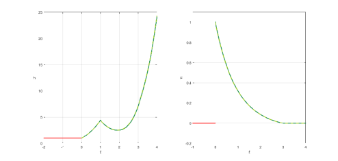
Figure 1. Optimal solution of problem (3.3): red line – initial data; dark green line – analytical solution; dashed light green line – numerical solution.

4. Delayed non-linear optimal control problem

This section is devoted to non-linear optimal control problems with constant time delays in state and control variables. We make a survey on a sufficient optimality condition for this type of problems. Its proof, and more details associated with the contents of the current section, can be found in [51]. We finish this section with an illustrative example.

4.1. Statement of the optimal control problem

We start by defining the delayed non-linear optimal control problem.

Definition 4.1.

Consider that $r\geq 0$ and $s\geq 0$ are constant time delays associated with the state and control variables, respectively. A non-autonomous optimal control problem with constant time delays and with a fixed initial state, on a fixed finite time interval $[a,b]$, is denoted by (OCP${}_{\text{D}}$) and consists in

$$\min\ \ C_{D}\big{(}x(\cdot),u(\cdot)\big{)}=g^{0}\big{(}x(b)\big{)}+\int_{a}^{b}f^{0}\big{(}t,x(t),x(t-r),u(t),u(t-s)\big{)}dt$$

subject to the delayed differential system

$$\dot{x}(t)=f\big{(}t,x(t),x(t-r),u(t),u(t-s)\big{)}\quad\text{for a.e.}\quad t\in[a,b]$$ (4.1)

with initial and final conditions

$$\begin{split}x(t)&=\varphi(t),\quad t\in[a-r-s,a]\subset\mathbb{R},\\ u(t)&=\psi(t),\quad t\in[a-s,a[,\\ x(b)&\in\Pi\subseteq\mathbb{R}^{n};\end{split}$$ (4.2)

where

1. the state trajectory is $x(t)\in\mathbb{R}^{n}$ for all $t\in[a-r-s,b]$;

2. the control is $u(t)\in U\subseteq\mathbb{R}^{m}$ for all $t\in[a-s,b]$;

3. $f=\left[\begin{matrix}f_{1}&\cdots&f_{n}\end{matrix}\right]^{T}$.

Next we define admissible pair for (OCP${}_{\text{D}}$).

Definition 4.2.

We say that $\big{(}x(\cdot),u(\cdot)\big{)}$ is an admissible pair for (OCP${}_{\text{D}}$) if it respects the following conditions:

1. $\big{(}x(\cdot),u(\cdot)\big{)}\in W^{1,\infty}\big{(}[a-r-s,b],\mathbb{R}^{n}\big{)}\times L^{\infty}\big{(}[a-s,b],\mathbb{R}^{m}\big{)}$;

2. $\big{(}x(\cdot),u(\cdot)\big{)}$ satisfies conditions (4.1) and (4.2);

3. $\big{(}x(t),u(t)\big{)}\in\mathbb{R}^{n}\times U$ for all $t\in[a,b]$.

4.2. Main result

In what follows we also consider that the time delays $r$ and $s$ respect Commensurability Assumption 2.1. Moreover, here we use Notations 2.2 and 2.3.

The following theorem provides a sufficient optimality condition associated with (OCP${}_{\text{D}}$) (see Definition 4.1). Such result generalizes Theorem 7 in Chapter 5.2 of [47].

Theorem 4.3.

Consider (OCP${}_{\text{D}}$). Let the interval $[a,b]$ be divided into $N\in\mathbb{N}$ subintervals of amplitude $h=\frac{b-a}{N}>0$ and suppose that the functions $g^{0}$, $f^{0}$ and $f$ are of class $\mathcal{C}^{1}$ with respect to all their arguments. Assume there exists a $\mathcal{C}^{1}\left(\mathbb{R}^{1+3n},\mathbb{R}^{m}\right)$ feedback control $u^{*}\Big{(}t,x_{r}(t),\eta\big{(}t,x_{r}(t)\big{)}\Big{)}=u^{*}[x,\eta]_{r}(t)$ such that

$$\begin{split}&\ \max_{u\in U}\Big{\{}H\Big{(}t,x_{r}(t),u,u^{*}[x,\eta]_{r}(t_{s}),\eta\big{(}t,x_{r}(t)\big{)}\Big{)}\\ &\ +H\Big{(}t^{s},x_{r}(t^{s}),u^{*}[x,\eta]_{r}(t^{s}),u,\eta\big{(}t^{s},x_{r}(t^{s})\big{)}\Big{)}\chi_{[a,b-s]}(t)\Big{\}}\\ =&\ H\Big{(}t,x_{r}(t),u^{*}[x,\eta]_{r}(t),u^{*}[x,\eta]_{r}(t_{s}),\eta\big{(}t,x_{r}(t)\big{)}\Big{)}\\ &\ +H\Big{(}t^{s},x_{r}(t^{s}),u^{*}[x,\eta]_{r}(t^{s}),u^{*}[x,\eta]_{r}(t),\eta\big{(}t^{s},x_{r}(t^{s})\big{)}\Big{)}\chi_{[a,b-s]}(t)\\ =:&\ H^{0}[x,\eta]_{r}(t)+H^{0}[x,\eta]_{r}(t^{s})\chi_{[a,b-s]}(t)\end{split}$$

for all $t\in[a,b]$, where

$$H(t,x,y,u,v,\eta)=-f^{0}(t,x,y,u,v)+\eta f(t,x,y,u,v).$$

Furthermore, let $I_{i}=[a+hi,a+h(i+1)]$, $i=0,\ldots,N-1$, and suppose that function $S\big{(}t,x(t)\big{)}\in\mathcal{C}^{2}\left(\mathbb{R}^{1+n},\mathbb{R}\right)$, $t\in[a,b]$, is a solution of equation

$$\begin{split}&\ \partial_{1}S\big{(}t,x(t)\big{)}+\sum_{i=0}^{N-1}\Big{\{}-f^{0}\big{(}t,x_{r}(t),u^{*}\langle x,\partial_{2}S\rangle_{r}(t),u^{*}\langle x,\partial_{2}S\rangle_{r}(t_{s})\big{)}\\ &+\partial_{2}S\big{(}t,x(t)\big{)}f\big{(}t,x_{r}(t),u^{*}\langle x,\partial_{2}S\rangle_{r}(t),u^{*}\langle x,\partial_{2}S\rangle_{r}(t_{s})\big{)}\Big{\}}\chi_{I_{i}}(t)=0\end{split}$$ (4.3)

with $S\big{(}b,x(b)\big{)}=-g^{0}\big{(}x(b)\big{)}$, $x(b)\in\Pi$. Finally, consider that the control law

$$u^{*}\Big{(}t,x_{r}(t),\partial_{2}S\big{(}t,x(t)\big{)}\Big{)}=u^{*}\langle x,\partial_{2}S\rangle_{r}(t),\quad t\in[a,b],$$

determines a response $\tilde{x}(t)$ steering $(a,x_{a})$ to $(b,\Pi)$. Then,

$$\tilde{u}(t)=u^{*}\big{(}t,\tilde{x}(t),\tilde{x}(t-r),\partial_{2}S(t,\tilde{x}(t)\big{)}$$

is an optimal control of (OCP${}_{\text{D}}$) that leads to the minimal cost

$$C_{D}\big{(}\tilde{x}(\cdot),\tilde{u}(\cdot)\big{)}=-S(a,x_{a}).$$

The detailed proof of Theorem 4.3 can be found in [51].

4.3. An illustrative example

In this section we provide an example of application of Theorem 4.3.

Let us consider the following delayed non-linear optimal control problem studied by Göllmann et al. in [26]:

$$\begin{split}\min\ \ \ &C_{D}\big{(}x(\cdot),u(\cdot)\big{)}=\int_{0}^{3}x^{2}(t)+u^{2}(t)dt,\\ \text{s.t.}\ \ &\dot{x}(t)=x(t-1)\ u(t-2),\\ &x(t)=1,\quad t\in[-1,0],\\ &u(t)=0,\quad t\in[-2,0[,\end{split}$$ (4.4)

which is a particular case of our delayed non-linear optimal control problem (OCP${}_{\text{D}}$) with $n=m=1$, $a=0$, $b=3$, $r=1$, $s=2$, $g^{0}\big{(}x(3)\big{)}=0$, $f^{0}(t,x,y,u,v)=x^{2}+u^{2}$ and $f(t,x,y,u,v)=yv$. In [26], necessary optimality conditions were proved and applied to (4.4). The following candidate $\big{(}x^{*}(\cdot),u^{*}(\cdot)\big{)}$ was found:

$$\begin{split}x^{*}(t)=\begin{cases}1,\ &t\in[-1,2],\\[8.00003pt] \displaystyle\frac{e^{t-2}+e^{4-t}}{e^{2}+1},\ &t\in\ [2,3],\end{cases}\end{split}$$ (4.5)

and

$$\begin{split}u^{*}(t)=\begin{cases}0,\ &t\in[-2,0[,\\[8.00003pt] \displaystyle\frac{e^{t}-e^{2-t}}{e^{2}+1},\ &t\in[0,1],\\[8.00003pt] 0,\ &t\in\ [1,3].\end{cases}\end{split}$$ (4.6)

It remains missing in [26], however, a proof that such candidate (4.5)–(4.6) is a solution to the problem. It follows from our sufficient optimality condition that such claim is indeed true.

We denote that $x_{0}^{*}(t)=1$, $t\in[-1,0]$; $x_{1}^{*}(t)=1$, $t\in[0,1]$; $x_{2}^{*}(t)=1$, $t\in[1,2]$; $x_{3}^{*}(t)=\frac{e^{t-2}+e^{4-t}}{e^{2}+1}$, $t\in[2,3]$; $u_{0}^{*}(t)=0$, $t\in[-2,0[$; $u_{1}^{*}(t)=\frac{e^{t}-e^{2-t}}{e^{2}+1}$, $t\in[0,1]$; $u_{2}^{*}(t)=0$, $t\in[1,2]$ and $u_{3}^{*}(t)=0$, $t\in[2,3]$. Furthermore, the corresponding adjoint function is given by

$$\begin{split}\eta(t)=&\begin{cases}\eta_{1}(t),\ &t\in[0,1]\\[8.00003pt] \eta_{2}(t),\ &t\in[1,2]\\[8.00003pt] \eta_{3}(t),\ &t\in[2,3]\end{cases}\\ =&\begin{cases}-2t+5+\dfrac{2\big{(}e^{2}-1\big{)}}{\big{(}e^{2}+1\big{)}^{2}},\ &t\in[0,1]\\[13.99995pt] -\left(\dfrac{4e^{2}}{\big{(}e^{2}+1\big{)}^{2}}+2\right)t+\dfrac{4\big{(}e^{2}-1\big{)}}{\big{(}e^{2}+1\big{)}^{2}}+6+\dfrac{e^{2t-2}-e^{6-2t}}{\big{(}e^{2}+1\big{)}^{2}},\ &t\in[1,2]\\[13.99995pt] \dfrac{2\big{(}e^{4-t}-e^{t-2}\big{)}}{e^{2}+1},\ &t\in[2,3].\end{cases}\end{split}$$

From now on, we are going to ensure that these functions satisfy the sufficient optimality conditions studied in this section (see Theorem 4.3). So, for $t\in[0,3]$, we intend to find a function $S(t,x)$ that is a solution of equation (4.3) with $S\big{(}3,x(3)\big{)}=0$. As $\eta(t)=\partial_{2}S\big{(}t,x(t)\big{)}$, we obtain that

$$\begin{split}S(t,x)=\begin{cases}\eta_{1}(t)x+c_{1}(t),\ &t\in[0,1]\\[8.00003pt] \eta_{2}(t)x+c_{2}(t),\ &t\in[1,2]\\[8.00003pt] \eta_{3}(t)x+c_{3}(t),\ &t\in[2,3],\end{cases}\end{split}$$

where $c_{i}(\cdot)$ is a real function of real variable, $i\in\{1,2,3\}$. For $t\in[2,3]$, the equation (4.3) implies that

$$\ \dot{\eta_{3}}(t)x^{*}(t)+\dot{c_{3}}(t)-\big{(}x^{*2}(t)+u^{*2}(t)\big{)}+\eta_{3}(t)x^{*}(t-1)u^{*}(t-2)=0$$

$$\Leftrightarrow \ \dot{\eta_{3}}(t)x_{3}^{*}(t)+\dot{c_{3}}(t)-\big{(}x_{3}^{*2}(t)+u_{3}^{*2}(t)\big{)}+\eta_{3}(t)x_{2}^{*}(t-1)u_{1}^{*}(t-2)=0$$

$$\Leftrightarrow -\frac{2\left(e^{4-t}+e^{t-2}\right)}{e^{2}+1}\times\frac{e^{t-2}+e^{4-t}}{e^{2}+1}+\dot{c_{3}}(t)-\left(\frac{e^{t-2}+e^{4-t}}{e^{2}+1}\right)^{2}$$

$$+\eta_{3}(t)\times 1\times\frac{e^{t-2}-e^{2-(t-2)}}{e^{2}+1}=0$$

$$\Leftrightarrow \ \dot{c_{3}}(t)=\frac{5\big{(}e^{2t-4}+e^{8-2t}\big{)}+2e^{2}}{\big{(}e^{2}+1\big{)}^{2}}$$ (4.7)

with $S\big{(}3,x(3)\big{)}=c_{3}(3)=0$. Solving the differential equation (4.3) with final condition $c_{3}(3)=0$, we obtain that

$$c_{3}(t)=\frac{4e^{2}(t-3)+5\big{(}e^{2t-4}-e^{8-2t}\big{)}}{2\big{(}e^{2}+1\big{)}^{2}}.$$

For $t\in[1,2]$, the equation (4.3) implies that

$$\ \dot{\eta_{2}}(t)x^{*}(t)+\dot{c_{2}}(t)-\big{(}x^{*2}(t)+u^{*2}(t)\big{)}+\eta_{2}(t)x^{*}(t-1)u^{*}(t-2)=0$$

$$\Leftrightarrow \ \dot{\eta_{2}}(t)x_{2}^{*}(t)+\dot{c_{2}}(t)-\big{(}x_{2}^{*2}(t)+u_{2}^{*2}(t)\big{)}+\eta_{2}(t)x_{1}^{*}(t-1)u_{0}^{*}(t-2)=0$$

$$\Leftrightarrow \ -\left(\frac{4e^{2}}{\big{(}e^{2}+1\big{)}^{2}}+2\right)+\frac{2\big{(}e^{2t-2}+e^{6-2t}\big{)}}{\big{(}e^{2}+1\big{)}^{2}}+\dot{c_{2}}(t)-1+\eta_{2}(t)\times 1\times 0=0$$

$$\Leftrightarrow \ \dot{c_{2}}(t)=-\dfrac{2\big{(}e^{2t-2}+e^{6-2t}-5e^{2}\big{)}-3\big{(}e^{4}+1\big{)}}{\big{(}e^{2}+1\big{)}^{2}}$$ (4.8)

with $\eta_{2}(2)x_{2}^{*}(2)+c_{2}(2)=\eta_{3}(2)x_{3}^{*}(2)+c_{3}(2)$, because $S\big{(}t,x(t)\big{)}\in\mathcal{C}^{2}\left(\mathbb{R}^{2},\mathbb{R}\right)$. Therefore, the previous condition is equivalent to

$$c_{2}(2)=c_{3}(2)=\frac{5\big{(}1-e^{4}\big{)}-4e^{2}}{2\big{(}e^{2}+1\big{)}^{2}}.$$ (4.9)

Solving the differential equation (4.3) with the condition (4.9), we have that

$$c_{2}(t)=\frac{2t\big{(}3e^{4}+10e^{2}+3\big{)}+2\big{(}e^{6-2t}-e^{2t-2}\big{)}-17e^{4}-44e^{2}-7}{2\big{(}e^{2}+1\big{)}^{2}}.$$

For $t\in[0,1]$, the equation (4.3) implies that

$$\ \dot{\eta_{1}}(t)x^{*}(t)+\dot{c_{1}}(t)-\big{(}x^{*2}(t)+u^{*2}(t)\big{)}+\eta_{1}(t)x^{*}(t-1)u^{*}(t-2)=0$$

$$\Leftrightarrow \ \dot{\eta_{1}}(t)x_{1}^{*}(t)+\dot{c_{1}}(t)-\big{(}x_{1}^{*2}(t)+u_{1}^{*2}(t)\big{)}+\eta_{1}(t)x_{0}^{*}(t-1)u_{0}^{*}(t-2)=0$$

$$\Leftrightarrow -2+\dot{c_{1}}(t)-1-\left(\frac{e^{t}-e^{2-t}}{e^{2}+1}\right)^{2}+\eta_{1}(t)\times 1\times 0=0$$

$$\Leftrightarrow \ \dot{c_{1}}(t)=\frac{e^{4-2t}+e^{2t}+3e^{4}+4e^{2}+3}{\big{(}e^{2}+1\big{)}^{2}}$$ (4.10)

with $\eta_{1}(1)x_{1}^{*}(1)+c_{1}(1)=\eta_{2}(1)x_{2}^{*}(1)+c_{2}(1)$, because $S\big{(}t,x(t)\big{)}\in\mathcal{C}^{2}\left(\mathbb{R}^{2},\mathbb{R}\right)$. Therefore, the previous condition is equivalent to

$$c_{1}(1)=c_{2}(1)=\frac{-9e^{4}-24e^{2}-3}{2\big{(}e^{2}+1\big{)}^{2}}.$$ (4.11)

Solving the differential equation (4.3) with the condition (4.11), we obtain that

$$c_{1}(t)=\frac{2t\big{(}3e^{4}+4e^{2}+3\big{)}+e^{2t}-e^{4-2t}-15e^{4}-32e^{2}-9}{2\big{(}e^{2}+1\big{)}^{2}}.$$

Concluding, the previous computations show the following result.

Proposition 4.4.

Function

$$\begin{split}S(t,x)=\begin{cases}\eta_{1}(t)x+c_{1}(t),\ &t\in[0,1],\\[8.00003pt] \eta_{2}(t)x+c_{2}(t),\ &t\in[1,2],\\[8.00003pt] \eta_{3}(t)x+c_{3}(t),\ &t\in[2,3],\end{cases}\end{split}$$

with

$$\begin{split}\eta_{1}(t)&=-2t+5+\dfrac{2\big{(}e^{2}-1\big{)}}{\big{(}e^{2}+1\big{)}^{2}},\\ \eta_{2}(t)&=-\left(\dfrac{4e^{2}}{\big{(}e^{2}+1\big{)}^{2}}+2\right)t+\dfrac{4\big{(}e^{2}-1\big{)}}{\big{(}e^{2}+1\big{)}^{2}}+6+\dfrac{e^{2t-2}-e^{6-2t}}{\big{(}e^{2}+1\big{)}^{2}},\\ \eta_{3}(t)&=\dfrac{2\big{(}e^{4-t}-e^{t-2}\big{)}}{e^{2}+1},\end{split}$$

and

$$\begin{split}c_{1}(t)&=\frac{2t\big{(}3e^{4}+4e^{2}+3\big{)}+e^{2t}-e^{4-2t}-15e^{4}-32e^{2}-9}{2\big{(}e^{2}+1\big{)}^{2}},\\ c_{2}(t)&=\frac{2t\big{(}3e^{4}+10e^{2}+3\big{)}+2\big{(}e^{6-2t}-e^{2t-2}\big{)}-17e^{4}-44e^{2}-7}{2\big{(}e^{2}+1\big{)}^{2}},\\ c_{3}(t)&=\frac{4e^{2}(t-3)+5\big{(}e^{2t-4}-e^{8-2t}\big{)}}{2\big{(}e^{2}+1\big{)}^{2}},\end{split}$$

is solution of the Hamilton–Jacobi equation (4.3) with $S\big{(}3,x^{*}(3)\big{)}=0$.

5. Conclusion

In this work we did a detailed state of the art associated with optimality conditions for delayed optimal control problems. Our survey ends with sufficient optimality conditions for two different types of delayed optimal control problems that are, to the best of our knowledge, the first to give an answer to a long-standing open question. Since the proofs are long, technical, and can be found in [50, 51], we did not present them here. However, examples were provided with the purpose to illustrate the usefulness of Theorems 3.3 and 4.3. As future work, we plan to show the usefulness of our results to control infectious diseases.

References

- [1] V. L. Bakke, Optimal fields for problems with delays. J. Optim. Theory Appl. 33(1) (1981), 69–84.
- [2] H. T. Banks, Necessary conditions for control problems with variable time lags. SIAM J. Control 6 (1968), 9–47.
- [3] E. B. M. Bashier K. C. Patidar, Optimal control of an epidemiological model with multiple time delays. Appl. Math. Comput. 292 (2017), 47–56.
- [4] M. Basin J. Rodriguez-Gonzalez, Optimal control for linear systems with multiple time delays in control input. IEEE Trans. Automat. Control 51(1) (2006), 91–97.
- [5] M. Benharrat D. F. M. Torres, Optimal control with time delays via the penalty method. Math. Probl. Eng. (2014), Art. ID 250419, 9 pp. arXiv:1407.5168
- [6] A. Boccia, P. Falugi, H. Maurer R. Vinter, Free time optimal control problems with time delays. 52nd IEEE Conference on Decision and Control (2013), 520–525.
- [7] A. Boccia R. B. Vinter, The maximum principle for optimal control problems with time delays. SIAM J. Control Optim. 55(5) (2017), 2905–2935.
- [8] G. V. Bokov, Pontryagin’s maximum principle in a problem with time delay. Fundam. Prikl. Mat. 15(5) (2009), 3–19.
- [9] F. Cacace, F. Conte, A. Germani G. Palombo, Optimal control of linear systems with large and variable input delays. Systems Control Lett. 89 (2016), 1–7.
- [10] G. Carlier R. Tahraoui, Hamilton-Jacobi-Bellman equations for the optimal control of a state equation with memory. ESAIM Control Optim. Calc. Var. 16(3) (2010), 744–763.
- [11] W. L. Chan S. P. Yung, Sufficient conditions for variational problems with delayed argument. J. Optim. Theory Appl. 76(1) (1993), 131–144.
- [12] L. Chen, K. Hattaf and J. Sun, Optimal control of a delayed SLBS computer virus model. Phys. A 427 (2015), 244–250.
- [13] D. H. Chyung E. B. Lee, Linear optimal systems with time delays. SIAM J. Control 4 (1966), 548–575.
- [14] A. Debbouche D. F. M. Torres, Approximate controllability of fractional nonlocal delay semilinear systems in Hilbert spaces. Internat. J. Control 86(9) (2013), 1577–1585. arXiv:1304.0082
- [15] A. Debbouche D. F. M. Torres, Approximate controllability of fractional delay dynamic inclusions with nonlocal control conditions. Appl. Math. Comput. 243 (2014), 161–175. arXiv:1405.6591
- [16] M. C. Delfour, The linear-quadratic optimal control problem with delays in state and control variables: a state space approach. SIAM J. Control Optim. 24(5) (1986), 835–883.
- [17] A. M. Elaiw N. H. AlShamrani, Stability of a general delay-distributed virus dynamics model with multi-staged infected progression and immune response. Math. Methods Appl. Sci. 40(3) (2017), 699–719.
- [18] D. H. Eller, J. K. Aggarwal H. T. Banks, Optimal control of linear time-delay systems. IEEE Trans. Automat. Control AC-14 (1969), 678–687.
- [19] G. S. F. Frederico, T. Odzijewicz D. F. M. Torres, Noether’s theorem for non-smooth extremals of variational problems with time delay. Appl. Anal. 93(1) (2014), 153–170. arXiv:1212.4932
- [20] G. S. F. Frederico D. F. M. Torres, Noether’s symmetry theorem for variational and optimal control problems with time delay. Numer. Algebra Control Optim. 2(3) (2012), 619–630. arXiv:1203.3656
- [21] G. S. F. Frederico D. F. M. Torres, A nondifferentiable quantum variational embedding in presence of time delays. Int. J. Difference Equ. 8(1) (2013), 49–62. arXiv:1211.4391
- [22] A. Friedman, Optimal control for hereditary processes. Arch. Rational Mech. Anal. 15 (1964), 396–416.
- [23] M. Fuhrman, F. Masiero G. Tessitore, Stochastic equations with delay: optimal control via BSDEs and regular solutions of Hamilton-Jacobi-Bellman equations. SIAM J. Control Optim. 48(7) (2010), 4624–4651.
- [24] D. M. Gay, The AMPL modeling language: an aid to formulating and solving optimization problems. In: Numerical analysis and optimization, vol. 134, Springer Proc. Math. Stat., pp. 95–116. Springer, Cham, 2015.
- [25] B. Goldys F. Gozzi, Second order parabolic Hamilton-Jacobi-Bellman equations in Hilbert spaces and stochastic control: approach. Stochastic Process. Appl. 116(12) (2006), 1932–1963.
- [26] L. Göllmann, D. Kern H. Maurer, Optimal control problems with delays in state and control variables subject to mixed control-state constraints. Optimal Control Appl. Methods 30(4) (2009), 341–365.
- [27] L. Göllmann H. Maurer, Theory and applications of optimal control problems with multiple time-delays. J. Ind. Manag. Optim. 10(2) (2014), 413–441.
- [28] T. Guinn, Reduction of delayed optimal control problems to nondelayed problems. J. Optimization Theory Appl. 18(3) (1976), 371–377.
- [29] A. Halanay, Optimal controls for systems with time lag. SIAM J. Control 6 (1968), 215–234.
- [30] G. L. Haratišvili, The maximum principle in the theory of optimal processes involving delay. Soviet Math. Dokl. 2 (1961), 28–32.
- [31] G. L. Haratišvili, A maximum principle in extremal problems with delays. In: Mathematical Theory of Control (Proc. Conf., Los Angeles, Calif., 1967), pp. 26–34. Academic Press, New York, 1967.
- [32] G. L. Haratišvili T. A. Tadumadze, Nonlinear optimal control systems with variable lags. Mat. Sb. (N.S.) 107(149)(4) (1978), 613–633, 640.
- [33] K. Hattaf N. Yousfi, Optimal control of a delayed HIV infection model with immune response using an efficient numerical method. Int. Schol. Res. Notices 2012 (2012), Art. ID 215124, 7 pp. https://doi.org/10.5402/2012/215124
- [34] M. R. Hestenes, On variational theory and optimal control theory. J. Soc. Indust. Appl. Math. Ser. A Control 3 (1965), 23–48.
- [35] D. K. Hughes, Variational and optimal control problems with delayed argument. J. Optimization Theory Appl. 2 (1968), 1–14.
- [36] S. H. Hwang Z. Bien, Sufficient conditions for optimal time-delay systems with applications to functionally constrained control problems. Internat. J. Control 38(3) (1983), 607–620.
- [37] A. F. Ivanov A. V. Swishchuk, Optimal control of stochastic differential delay equations with application in economics. Int. J. Qual. Theory Differ. Equ. Appl. 2(2) (2008), 201–213.
- [38] F. Ibrahim, K. Hattaf, F. A. Rihan S. Turek, Numerical method based on extended one-step schemes for optimal control problem with time-lags. Int. J. Dyn. Control 5(4) (2017), 1172–1181.
- [39] M. Q. Jacobs T. Kao, An optimum settling problem for time lag systems. J. Math. Anal. Appl. 40 (1972), 687–707.
- [40] F. Khellat, Optimal control of linear time-delayed systems by linear Legendre multiwavelets. J. Optim. Theory Appl. 143(1) (2009), 107–121.
- [41] J. Klamka, H. Maurer A. Swierniak, Local controllability and optimal control for a model of combined anticancer therapy with control delays. Math. Biosci. Eng. 14(1) (2017), 195–216.
- [42] R. W. Koepcke, On the control of linear systems with pure time delay. J. Basic Eng. 87(1) (1965), 74–80.
- [43] H. N. Koivo E. B. Lee, Controller synthesis for linear systems with retarded state and control variables and quadratic cost. Automatica–J. IFAC 8 (1972), 203–208.
- [44] B. Larssen, Dynamic programming in stochastic control of systems with delay. Stoch. Stoch. Rep. 74(3-4) (2002), 651–673.
- [45] C. H. Lee S. P. Yung, Sufficient conditions for optimal control problems with time delay. J. Optim. Theory Appl. 88(1) (1996), 157–176.
- [46] E. B. Lee, Variational problems for systems having delay in the control action. IEEE Trans. Automatic Control AC-13 (1968), 697–699.
- [47] E. B. Lee L. Markus, Foundations of optimal control theory. 2nd Edition, Robert E. Krieger Publishing Co., Inc., Melbourne, FL, 1986.
- [48] R. C. H. Lee S. P. Yung, Optimality conditions and duality for a non-linear time-delay control problem. Optimal Control Appl. Methods 18(5) (1997), 327–340.
- [49] A. P. Lemos-Paião, Introduction to optimal control theory and its application to diabetes. M.Sc. thesis, University of Aveiro, Portugal, 2015. http://hdl.handle.net/10773/16806
- [50] A. P. Lemos-Paião, C. J. Silva D. F. M. Torres, A sufficient optimality condition for delayed state-linear optimal control problems. Discrete Contin. Dyn. Syst. Ser. B 24(5) (2019), 2293–2313. arXiv:1901.04340
- [51] A. P. Lemos-Paião, C. J. Silva D. F. M. Torres, A sufficient optimality condition for non-linear delayed optimal control problems. Pure Appl. Funct. Anal. 4(2) (2019), 345–361. arXiv:1804.06937
- [52] A. B. Malinowska T. Odzijewicz, Second Noether’s theorem with time delay. Appl. Anal. 96(8) (2017), 1358–1378.
- [53] M. N. Oğuztöreli, A time optimal control problem for systems described by differential difference equations. J. Soc. Indust. Appl. Math. Ser. A Control 1 (1963), 290–310.
- [54] M. N. Oğuztöreli, Time-lag control systems, vol. 24, Mathematics in Science and Engineering. Academic Press, New York-London, 1966.
- [55] K. R. Palanisamy R. G. Prasada, Optimal control of linear systems with delays in state and control via Walsh functions. IEE Proceedings D – Control Theory and Applications 130(6) (1983), 300–312.
- [56] W. J. Palm W. E. Schmitendorf, Conjugate-point conditions for variational problems with delayed argument. J. Optimization Theory Appl. 14 (1974), 599–612.
- [57] H. Pirnay, R. López-Negrete L. T. Biegler, Optimal sensitivity based on IPOPT. Math. Program. Comput. 4(4) (2012), 307–331.
- [58] L. S. Pontryagin, V. G. Boltyanskii, R. V. Gamkrelidze E. F. Mishchenko, The mathematical theory of optimal processes. Translated from the Russian by K. N. Trirogoff; edited by L. W. Neustadt. Interscience Publishers John Wiley & Sons, Inc. New York-London, 1962.
- [59] V.-M. Popov, One problem in the theory of absolute stability of controlled systems. Automat. Remote Control 25 (1964), 1129–1134.
- [60] D. Rocha, C. J. Silva D. F. M. Torres, Stability and optimal control of a delayed HIV model. Math. Methods Appl. Sci. 41(6) (2018), 2251–2260. arXiv:1609.07654
- [61] F. Rodrigues, C. J. Silva, D. F. M. Torres H. Maurer, Optimal control of a delayed HIV model. Discrete Contin. Dyn. Syst. Ser. B 23(1) (2018), 443–458. arXiv:1708.06451
- [62] L. D. Sabbagh, Variational problems with lags. J. Optimization Theory Appl. 3 (1969), 34–51.
- [63] S. P. S. Santos, N. Martins D. F. M. Torres, Variational problems of Herglotz type with time delay: DuBois-Reymond condition and Noether’s first theorem. Discrete Contin. Dyn. Syst. 35(9) (2015), 4593–4610. arXiv:1501.04873
- [64] S. P. S. Santos, N. Martins D. F. M. Torres, Higher-order variational problems of Herglotz type with time delay. Pure Appl. Funct. Anal. 1(2) (2016), 291–307. arXiv:1603.04034
- [65] S. P. S. Santos, N. Martins D. F. M. Torres, Noether currents for higher-order variational problems of Herglotz type with time delay. Discrete Contin. Dyn. Syst. Ser. S 11(1) (2018), 91–102. arXiv:1704.00088
- [66] W. E. Schmitendorf, A sufficient condition for optimal control problems with time delays. Automatica – J. IFAC 9 (1973), 633–637.
- [67] C. J. Silva, H. Maurer D. F. M. Torres, Optimal control of a tuberculosis model with state and control delays. Math. Biosci. Eng. 14(1) (2017), 321–337. arXiv:1606.08721
- [68] M. A. Soliman, A new necessary condition for optimality of systems with time delay. J. Optimization Theory Appl. 11 (1973), 249–254.
- [69] E. Stumpf, Local stability analysis of differential equations with state-dependent delay. Discrete Contin. Dyn. Syst. 36(6) (2016), 3445–3461.
- [70] J. Xu, Y. Geng Y. Zhou, Global stability of a multi-group model with distributed delay and vaccination. Math. Methods Appl. Sci. 40(5) (2017), 1475–1486.
- [71] R. Xu, S. Zhang F. Zhang, Global dynamics of a delayed SEIS infectious disease model with logistic growth and saturation incidence. Math. Methods Appl. Sci. 39(12) (2016), 3294–3308.