Phase coherence and phase jumps in the Schwabe cycle

Abstract

Guided by the working hypothesis that the Schwabe cycle of solar activity is synchronized by the 11.07 years alignment cycle of the tidally dominant planets Venus, Earth and Jupiter, we reconsider the phase diagrams of sediment accumulation rates in lake Holzmaar, and of methanesulfonate (MSA) data in the Greenland ice core GISP2, which are available for the period 10000-9000 cal. BP. Since some half-cycle phase jumps appearing in the output signals are, very likely, artifacts of applying a biologically substantiated transfer function, the underlying solar input signal with a dominant 11.04 years periodicity can be considered as mainly phase-coherent over the 1000 years period in the early Holocene. For more recent times, we show that the re-introduction of a hypothesized “lost cycle” at the beginning of the Dalton minimum would lead to a real phase jump. Similarly, by analyzing various series of ¹⁴C and ¹⁰Be data and comparing them with Schove’s historical cycle maxima, we support the existence of another “lost cycle” around 1565, also connected with a real phase jump. Viewed synoptically, our results lend greater plausibility to the starting hypothesis of a tidally synchronized solar cycle, which at times can undergo phase jumps, although the competing explanation in terms of a non-linear solar dynamo with increased coherence cannot be completely ruled out.

1 Introduction

In hindsight, it is a mystery that the important paper of Vos et al. (2004) has been so widely overlooked in the solar physics community. Based on a careful selection of the 10000-9000 cal. BP segment of varved sediment accumulation data from lake Holzmaar (Vos et al. 1997), and employing a nonlinear transfer function reflecting the dependence of the biological productivity of autochthonous algae on temperature and/or solar radiation (in particular its UV component), the authors revealed strong evidence for a Schwabe cycle with a dominant 11.04 years period which was basically phase coherent over the considered 1000-year interval. The same periodicity and phase coherence was also detected in GRISP2 ice-core data, when analyzing the methanesulfonate (MSA) concentration as a marker of algal productivity in the North Atlantic. Some phase jumps by half a cycle (i.e. 5.5 years), showing up in both time series, appeared as artifacts of applying the transfer function, so that ultimately the input data of the underlying solar cycle was interpreted as phase coherent over 1000 years.

While such a long phase coherence, observed in two rather unrelated proxy data for the Schwabe cycle, is most remarkably in itself, one might be even more puzzled by the almost complete equivalence of the cycle period of 11.04 years with the corresponding 11.07-year period as derived for the last centuries (Stefani et al. 2019, 2020). Ironically, the latter value for the more recent times is more disputable than the value for the early Holocene, given that the systematic observation of sunspots goes back only to the times of Scheiner and Galileo (Arlt and Vaquero 2020), with grave uncertainties for the time of the Maunder minimum (1645-1715).

In an unparalleled effort of analyzing historical aurora borealis observations, Schove (1955, 1979, 1983) had tried to extend the widely accepted series of cycle minima and maxima to a much longer period of nearly two and a half millennia. The resulting time series prompted different reactions, ranging from appreciations of their high quality (Jelbring 1995) to less enthusiastic qualifications as being “archaic” (Usoskin 2017). With all due caveats about their reliableness, we recently analyzed Schove’s cycle maxima data down to A.D. 240 (where a first data gap appears), and found a clearly dominant and largely phase coherent cycle with a 11.07-years periodicity (Stefani et al. 2020), modulated by two longer cycles of the Suess-de Vries type (around 200 years) and the Gleissberg type (around 90 years). Moreover, analyzing Dicke’s ratio $\sum_{i}r_{i}^{2}/\sum_{i}(r_{i}-r_{i-1})^{2}$ (Dicke 1978) between the mean square of the residuals $r_{i}$ (defined as the distances between the actual minima and the hypothetical minima of a perfect 11.07-year cycle) to the mean square of the differences $r_{i}-r_{i-1}$ between two consecutive residuals, the solar cycle was shown to have much closer resemblance to a clocked process than to a random walk process (Stefani et al. 2019). This gave further support for our conjecture (Stefani et al. 2016, 2017, 2018, 2019) that the Schwabe cycle results from synchronizing a rather conventional $\alpha-\Omega$-dynamo by means of an additional 11.07-year oscillation of the $\alpha$-effect which, in turn, is related to the helicity oscillation of either a kink-type ($m=1$) Tayler instability in the tachocline region (Weber 2015) or a ($m=1$) magneto-Rossby wave (Dikpati 2017, Zaqarashvili 2018). Building on and corroborating earlier ideas of Hung (2007), Scafetta (2012), Wilson (2013), and Okhlopkov (2014, 2016), the source of this synchronized helicity was hypothesized to be the 11.07-year periodic tidal ($m=2$) forcing of Venus, Earth and Jupiter, which are the tidally dominant planets in the solar system.

While the hitherto overlooked 10000-9000 cal. BP data of Vos et al. (2004) seem to lend more plausibility to this tidal synchronization conjecture, there remain two objections against it which have to be considered seriously. The first question has to do with the possibility that the solar dynamo may undergo a sort of “self-synchronization”, with a phase-amplitude correlation resulting from the typical quenching of $\alpha-\Omega$-dynamos when exposed to random fluctuations of $\alpha$. As shown by Hoyng (1996) in a rebuttal to Dicke’s question “Is there a chronometer hidden deep in the sun?” (Dicke, 1978), the typical frequency-growth rate correlation of an $\alpha-\Omega$ dynamo could lead to a finite, yet rather long (hundreds of years) memory in conjunction with a stable phase coherence, which could be misinterpreted as a clocked process. More detailed investigations of such an increased coherence in a simple non-linear $\alpha-\Omega$ dynamo models are presently under way.

A second objection is related to the questionable quality of Schove’s minima and maxima data. While they show a remarkable phase coherence over one or even two millennia (Stefani et al. 2019, 2020), this coherence would be destroyed in case that Schove had forgotten (or “smuggled in”) one cycle or another. Sections 3 and 4 will deal with such “lost cycles” and the real phase jumps connected with them. However, before entering this issue we will shortly discuss some fictitious phase jumps appearing in the data of Vos et al. (2004).

2 Algae in the sun

Due to its key relevance to the synchronization theory of the solar dynamo, we reproduce Figure 17.7 of Vos et al. (2004) in our Figure 1. It shows the phase diagrams of varve thicknesses from Lake Holzmaar (a), and of methanesulfonate (MSA) influx measured in the Greenland ice core GISP2 (b), which had been produced by correlating the measured signal within a given comparison window (100 years) with an ideal sinusoidal signal of known periodicity and phase (more details about the creation of phase diagrams can be found in Appendix A). Both phase diagrams reveal the existence of two distinct band structures, phase shifted by half a cycle length (5.5 years), each of them lasting over intervals of one or a few hundred years. While, in general, the Holzmaar and the GISP2 data have a very similar appearance, their respective phase jumps are shifted systematically by 41 years due to the use of two different INTCAL calibration curves (Vos 2020). Later, we will also come back to the remarkable triangular structure which is visible in the GRISP2 data between 9800 and 9700 cal. BP, but not in the corresponding Holzmaar data. This point will also be critically assessed in Appendix A, where we elaborate on some sensitive parameter dependencies of phase diagrams such as Figure 1.

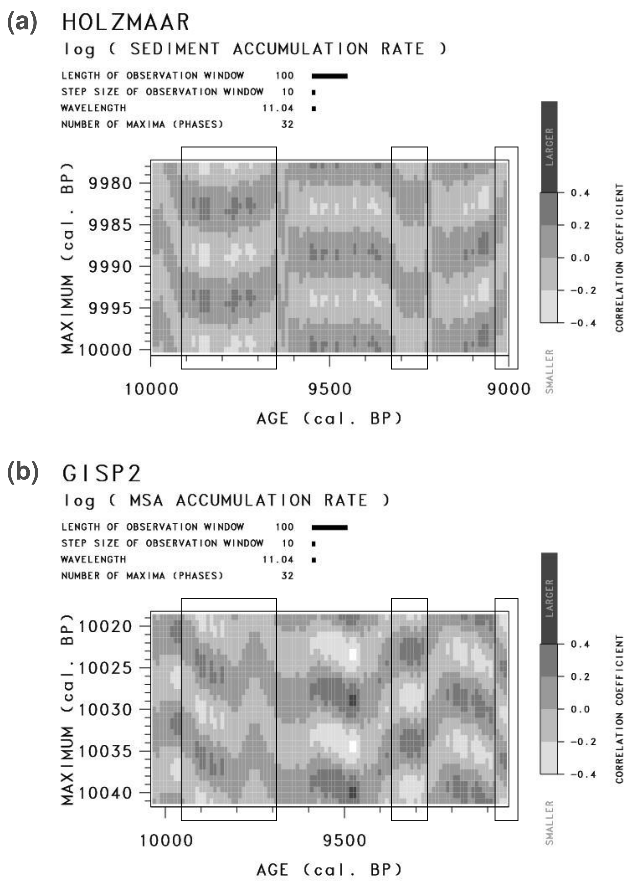
Figure 1: Reproduction of Figure 17.7 of Vos et al. (2004). Comparative phase analysis of varve thickness in Lake Holzmaar and MSA (Methanesulfonate) influx measured in the Greenland ice core of GISP2. (a) Phase diagram of varve thickness data of Lake Holzmaar between 10000 and 9000 cal. BP. (b) Phase diagram of MSA influx data from GISP2 between 10041 and 9041 cal. BP. Reprinted by permission from: Springer, Vos, H., Brüchmann, C., Lücke, A., Negendank, J.F.W., Schleser, G.H. & Zolitschka 2004, Climate in Historical Times: Towards a Synthesis of Holocene Proxy Data and Climate Models. H. Fischer, T. Kumke, G. Lohmann, G. Floser, H. Miller & H. von Storch (Eds.), GKSS School of Environmental Research, p. 293. Copyright (2004).

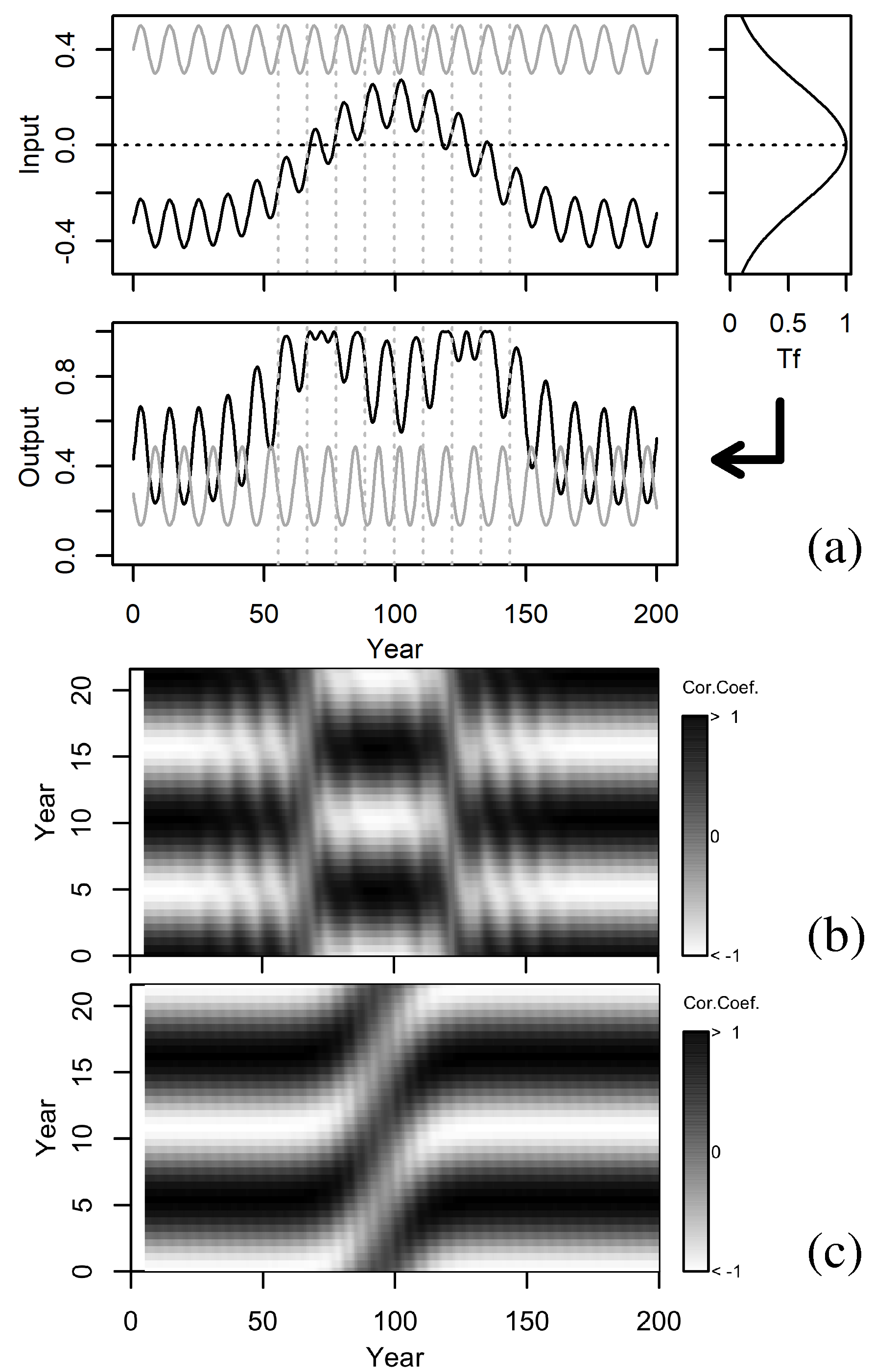
Figure 2: Illustration of the effect of a transfer function on signals without and with real phase jumps. (a) Two input functions, one (black) with a crossing of the maximum of the transfer function (right), the other one (gray) with an additional cycle around 100 years, are transferred into corresponding output signals. (b) Phase diagram of the output signal of the black curve from (a), with two apparent phase jumps by half a cycle. (c) Phase diagram of the output signal of the gray curve from (a), with one real phase jump by a full cycle.

As carefully worked out by Vos et al. (2004), such phase jumps by half a cycle should not be attributed to the underlying solar signal. Instead, they appear as artifacts of applying a nonlinear transfer function to the input signal related to solar activity. This transfer function reflects the optimality conditions of the growth of algae on abiotic input such as temperature or UV radiation. Adapting Figure 17.3 of Vos et al. (2004), the specific convolution effect of applying a transfer function to a signal comprising a high frequency and a secular trend is visualized here in Figure 2. We add to this, however, an illustration of the effect of a hypothetical real phase jump in the input data (as will be discussed further below) on the phase diagram. While such real phase jumps by 11 years in the input data would produce equivalent 11 years jumps in the phase diagram, this is not what was observed in Figure 1 (see, however, our discussion in Appendix A on the possibility that such fast phase jumps as in Figure 2c might have been missed in Figure 1 due to the long comparison window used by Vos et al. (2004)). At any rate, it seems quite plausible that the solar cycle was phase coherent over the central segment 9650-9350 cal. BP (if not the entire period 10000-9000 cal. BP) with a period of 11.04 years as estimated by Vos et al. (2004)). Given the limited accuracy and duration of the underlying datasets, we consider these 11.04 years as hardly distinguishable from the 11.07-year period to be discussed in the following (for the 90 cycles shown in Figure 1, this difference would result in a shift along the ordinate axis by 2.7 years).

3 Schove’s data and two “lost cycles”

We turn now to the Schwabe cycle during the last six centuries. Anticipating the limited availability of annual ¹⁴C and ¹⁰Be data (starting in the 16th and 15th century, respectively) we restrict the considered solar cycle maxima to those from A.D. 1404 onward (see Table 1). For the interval 1404 - 1755, we use the values from Table 2 and Appendix B of Schove (1983), whilst all later maxima (starting from 1761.5) are taken from the more contemporary Table 1 of Hathaway (2015) (they mainly coincide with Schove’s data, so that we indicate this series by the notion “Schove”). The maximum for the last cycle SC 24 has been roughly estimated to be 2013.0, which lies between the two activity peaks at the end of 2011 and the beginning of 2014. Basically, we utilize Wolf’s numbering scheme for the solar cycles, while possible candidates of “lost cycles” are indicated by half-integers, e.g. “-16.5” and “4.5”, the latter one corresponding to Usoskin’s notion “SC 4’ ” (Usoskin 2002).

Table 1: Maxima of solar cycles according to different sources. The two “lost cycles”, as discussed by Link (1978) and Usoskin et al. (2002), are included in the columns “Li/Us”.

SC	Schove	Li/Us	14C	Li/Us	10Be	Li/Us
-31	1404
-30	1416
-29	1428
-28	1439				1444
-27	1450				1454
-26	1460				1464
-25	1474				1471
-24	1485				1481
-23	1493				1494
-22	1506.5				1503
-21	1517.9		1524		1516
-20	1528.2		1532		1524
-19	1537.6		1541		1538
-18	1547.4		1551		1552
-17	1558.3	1555	1558		1558
-16.5		1563		1566		1567
-16	1571.3	1570	1576		1567	1577
-15	1581.5	1581	1584		1582
-14	1593.8		1593		1592
-13	1604.4		1603		1603
-12	1614.3		1613		1614
-11	1625.8		1626		1629
-10	1639.3		1638		1644
-9	1650.8		1646		1652
-8	1661.0		1655		1660
-7	1673.5		1664		1668
-6	1685.0		1675		1678
-5	1694.5		1690		1689
-4	1705.5		1704		1705
-3	1718.2		1719		1719
-2	1727.5		1730		1731
-1	1738.7		1740		1741
0	1750.3		1749		1751
1	1761.5		1762		1758
2	1769.75		1769		1765
3	1778.42		1781		1778
4	1788.17	1788.4	1791		1789
4.5		1795		1803		1801
5	1805.17	1802.5	1803	1812	1801	1812
6	1816.42	1817.1	1821		1820
7	1829.92		1830		1827
8	1837.25		1837		1837
9	1848.17		1852		1850
10	1860.17		1860		1861
11	1870.67		1870		1872
12	1884		1886		1886
13	1894.08		1895		1897
14	1906.17		1906		1907
15	1917.67		1918		1918
16	1928.33		1927		1927
17	1937.33		1938		1938
18	1947.42		1948		1948
19	1958.25		1959		1959
20	1968.92		1970
21	1980		1982
22	1989.58
23	2000.33
24	2013

The open squares in Figure 3 show the residuals of the times of the cycle maxima from a linear function with a hypothetical 11.07-year trend (this representation corresponds to the so-called “O$-$C”, i.e. “Observed minus Calculated” method, see Richards et al. 2009). Obviously, those residuals form a rather horizontal band, with the well-known tendency for shorter (and stronger) cycles in the 20th century. Particularly remarkable is also the accumulation of shorter cycles before the Dalton minimum, in combination with the following extremely long cycle SC 4, which brought the sequence of cycles back to the basic 11.07 periodicity. While this jumpy behaviour has been qualified as “great solar anomaly” (Sonett 1983), “irregular phase evolution” or “phase catastrophe” (Usoskin et al. 2002), we support here the quite contrary interpretation of Dicke (1978) that the abnormally long SC 4 simply re-establishes the phase coherence, after the few short cycles before were in danger of loosing synchronization. We note in passing that the rather weak SC 24 could play a similar role in re-synchronizing the series of cycles.

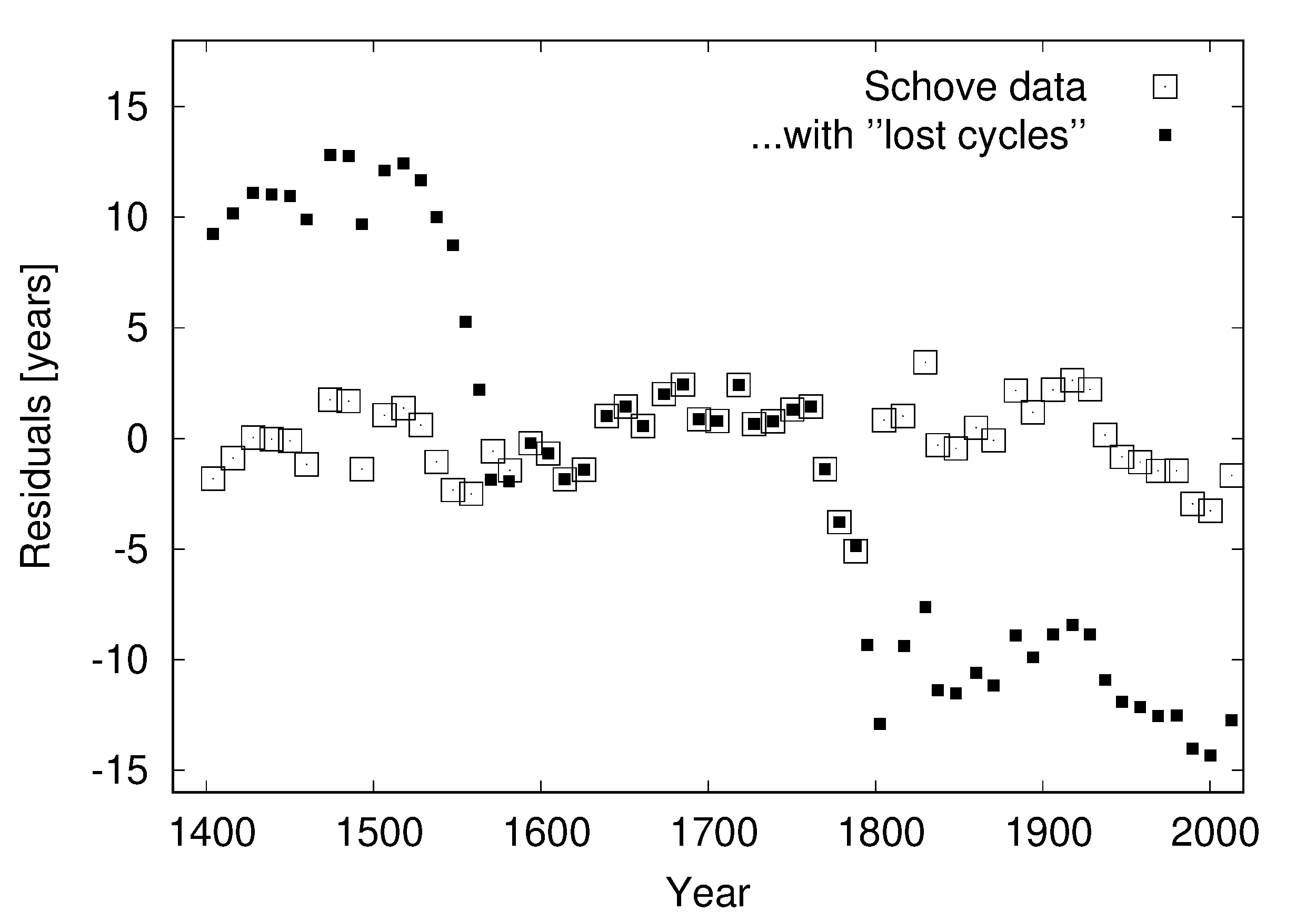
Figure 3: Residuals of Schove’s cycle maxima from a linear trend with 11.07-years period, without (open squares) and with inclusion (full squares) of the “lost cycles” of Link (1978) and Usoskin et al. (2002).

This being said, the quest for a “lost cycle” within SC 4 is perfectly legitimate, and Usoskin’s arguments for its existence were convincing, indeed (Usoskin 2002, Usoskin et al. 2009). If we add his additional maximum at 1795.0, and change also the instants of the neighboring maxima to Usoskin’s modified values, we obtain the full squares in Figure 3, showing now a sharp phase jump by 11.07 years.

The full squares in Figure 3 indicate also a second possible phase jump around 1563. The corresponding additional maximum had been derived by Link (1978) from auroral observations, but was deliberately omitted by Schove with the following justification: “An extra auroral cycle with a minimum in 1559 is due to the over-assiduous search for prodigies by Conrad Lycosthenes whose catalogue of prodigies ended at that time: in the Far East there is no corresponding minimum.” (Schove 1979). As we will see below, when analyzing cosmogenic isotopes, the occurrence of a (weak) maximum during this time is at least conceivable.

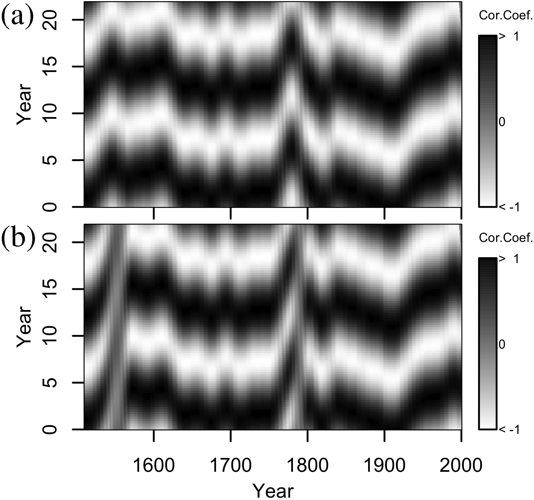
Figure 4: Phase diagrams of the maxima from Table 1, and the corresponding minima from Table A1, both for Schove’s original data (a) and for the inclusion of the “lost cycles” (b).

In Figure 4 we show the phase diagrams (generated in a similar way as Figure 17.7 of Vos et al. (2004), see Appendix A) of these two different time series. For that purpose we enhance the series of maxima according to Table 1 by the corresponding series of minima (see Table B1 in the appendix). However, since the reliability of Schove’s minima data is compromised before 1500 we restrict Figure 4 to the time period 1500-2000. Figure 4a shows the phase diagram for the pure Schove data, in Figure 4b we have included also the two “lost cycles”. The main difference between them is particularly visible shortly before 1800, where Schove’s data (a) exhibit a triangular shape, while the inclusion of the “lost cycle” makes this region appear more like the typical phase jump illustrated in Figure 2c. The triangular shape in Figure 4a is quite similar to the one seen in the 9800-9700 cal. BP segment (Figure 1b) of the GRISP2 date, while the corresponding segment of the Lake Holzmaar data (Figure 1a) did not show such a behaviour (but see, again, our critical discussion in Appendix A).

With Figure 5 we would like to point out an interesting effect - or better: a non-effect - of phase jumps. This figure shows the most relevant segment (more details can be found in Stefani et al. 2020) of the Lomb-Scargle diagram of the combined maxima and minima data, again for the data without and with the “lost cycles”. Somewhat contrary to a naive expectation (based on a simple counting of maxima in a certain time interval), the dominant peak at 11.07 years remains nearly unaffected by the inclusion of the “lost cycles”. The reason for that is the maintenance of phase coherence over the additional cycle, so that the projection of the data onto a test harmonic function does barely change.

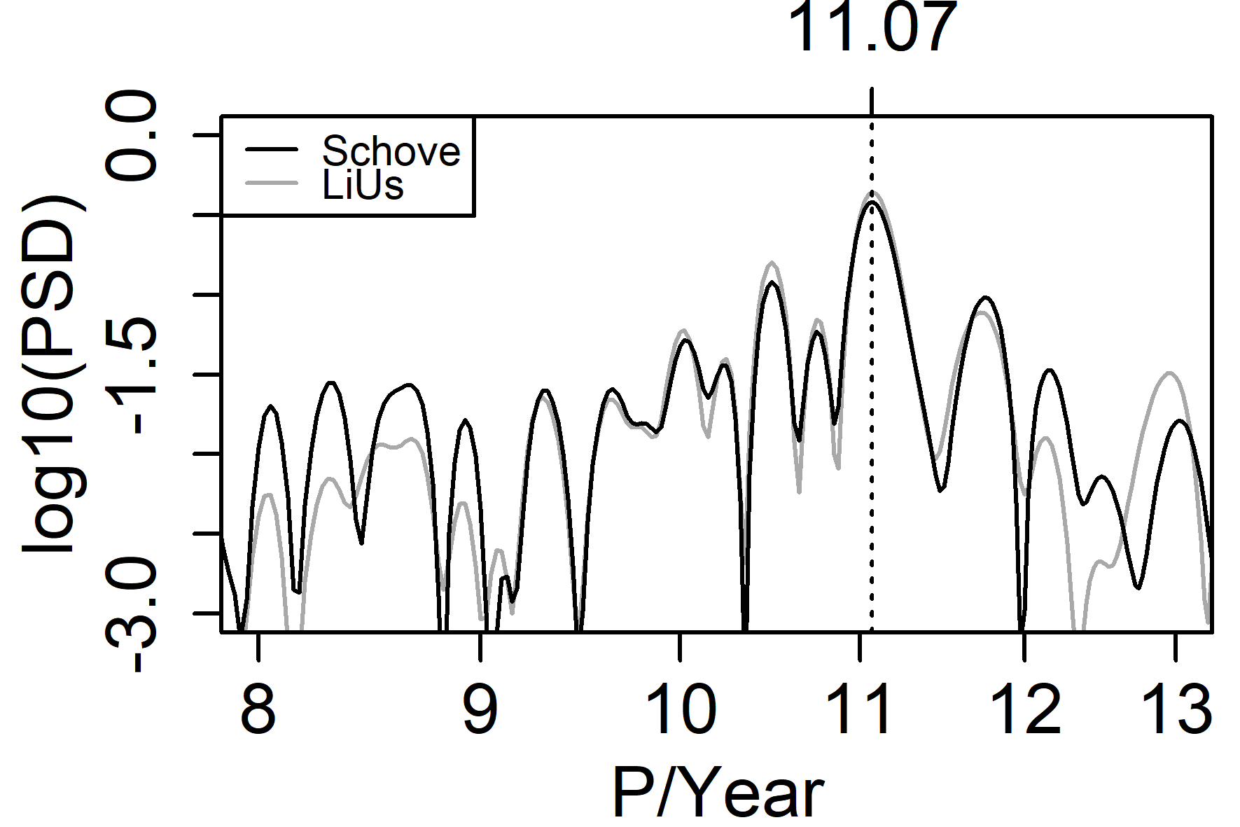
Figure 5: Zoom of the Lomb-Scargle diagram for the cycle maxima and minima corresponding to Schove’s data without (black) and with (gray) inclusion of the “lost cycles”. For the generation of the diagram, consecutive minima and maxima were smoothly connected by segments of sine-functions.

Note that those candidate phase jumps around 1565 and 1795 do in no way contradict the concept of synchronization; similar phase jumps are actually well known from various frequency-locked systems (Pikovski et al. 2003). However, the presently available data do not allow a conclusive decision about their existence. In both cases the corresponding data (sunspot numbers and/or radioisotopes) exhibit a rather shallow maximum within a comparably long cycle, and there is a certain degree of ambiguity on whether to count this behaviour as an additional cycle or not. Note that secondary peaks within one cycle are not untypical for the solar dynamo, and they were regularly produced in our tidal synchronization model (see Figure 7 in Stefani et al. 2016). Unfortunately, for those historical maxima around 1565 and 1795 we do not have the sign information for the solar magnetic field, which would be required for a (final) distinction between just a secondary peak or a full-blown additional cycle. Maybe some future cycles will give us the opportunity to clearly identify phase jumps.

At any rate, as we have seen in the PSD’s of Figure 5, the consequences of (potential) phase jumps would be quite limited since the spectrum at the dominant frequency is barely changed. The most important point is the re-synchronization after those “special events”.

4 Cycle maxima from radionuclide data

In this section, we attempt an independent validation of Schove’s maxima data (whose early parts were mainly derived from aurora borealis data) by annually resolved data of cosmogenic isotopes. Past solar activity has often been reconstructed using abundances of ¹⁴C or ¹⁰Be measured in stratified ice cores or (ancient) tree rings. These isotopes are constantly being produced in the Earth’s atmosphere due to interactions of oxygen and/or nitrogen with neutrons that in turn are generated from cosmic rays penetrating the upper layers of the atmosphere. The corresponding production rates of the isotopes depend on the flux of the cosmic rays, which is modulated by the periodically changing solar magnetic field. A comprehensive modeling of the involved processes includes the impact of secular long term variations due to changes in the Earth’s magnetic field, the typical residence time of isotopes in different layers of the atmosphere, as well as geophysical and climatic mechanisms. The resulting production rates proved to correlate well with the observed sunspot numbers (Beer et al. 2012, 2018), which in turn permits the reconstruction of solar activity cycle in time periods when no sunspot observations are available.

Specifically, we will use the solar modulation function $\Phi$ as derived by Muscheler et al. (2007), which mainly relies on ¹⁴C data from tree-rings, and two ¹⁰Be data sets of ice cores from the Dye-3 site (Beer et al. 1990) and the NGRIP site (Berggren et al. 2009) in Greenland. For both radionuclides we will outline our data processing scheme, including the splitting into moving averages and remainders. Later, when comparing the maxima resulting from those remainders with Schove’s data, we will discuss again the emergence of “lost cycles” as described in the previous section.

4.1 ¹⁴C data

We utilize the data of Muscheler et al. (2007,2008), and concentrate on their segment 1511-1954, where the data were basically inferred from the annual tree-ring ¹⁴C data of Stuiver et al. (1998). These were then transformed, taking into account a geomagnetic field reconstruction and a carbon cycle model, into a solar modulation potential with the unit MeV.

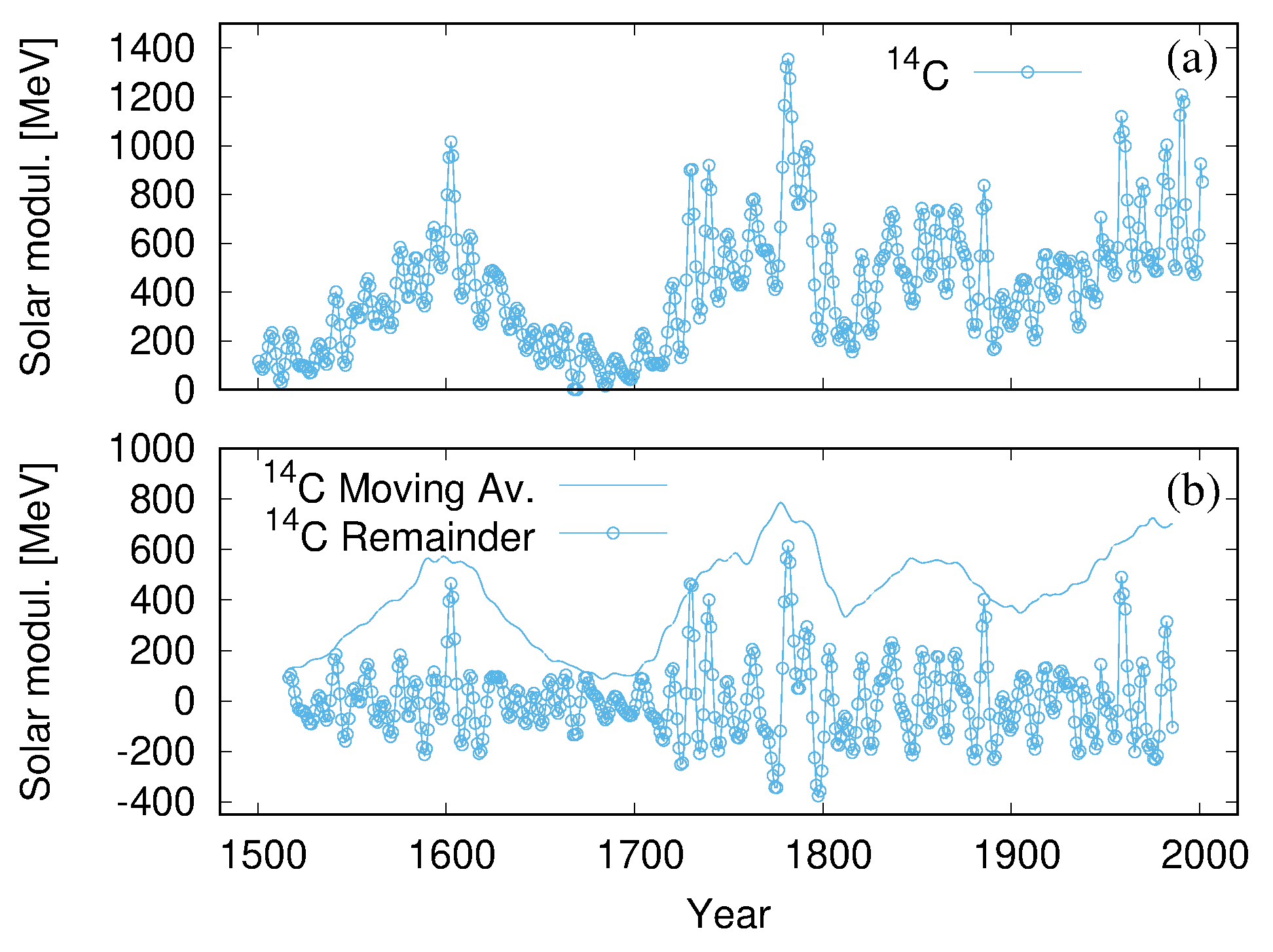
Figure 6: Solar modulation potential as derived from ¹⁴C data by Muscheler et al. (2008) (a), and the corresponding moving averages and remainders (b).

Figure 6 shows the original data of Muscheler et al. (2008), together with their splitting into a centered moving average (with an averaging period of 33 years) and the corresponding remainder. Only this remainder will be used below for the identification of the cycle maxima.

4.2 ¹⁰Be data

The first one of the two ¹⁰Be data sets stems from the site Dye 3 in South Greenland, originating from a 300-m ice core which represents approximately 600 years of ice accumulation. These data are given in a quasi-annual manner for the time period 1424 -1986 (Beer et al. 1990). Specifically, in Figure 7 we show the derived ¹⁰Be fluxes in units of atoms cm^-2 s^-1. Note that a specific segment between 1780-1886 had been used previously by Beer et al. (1990) to evidence a good anti-correlation with the sunspot numbers and the geomagnetic aa index, all dominated by a clear 11 years cycle of solar activity. Furthermore, the data had also been used to prove the uninterrupted presence of the solar cycle throughout the Maunder minimum (Beer et al. 1998).

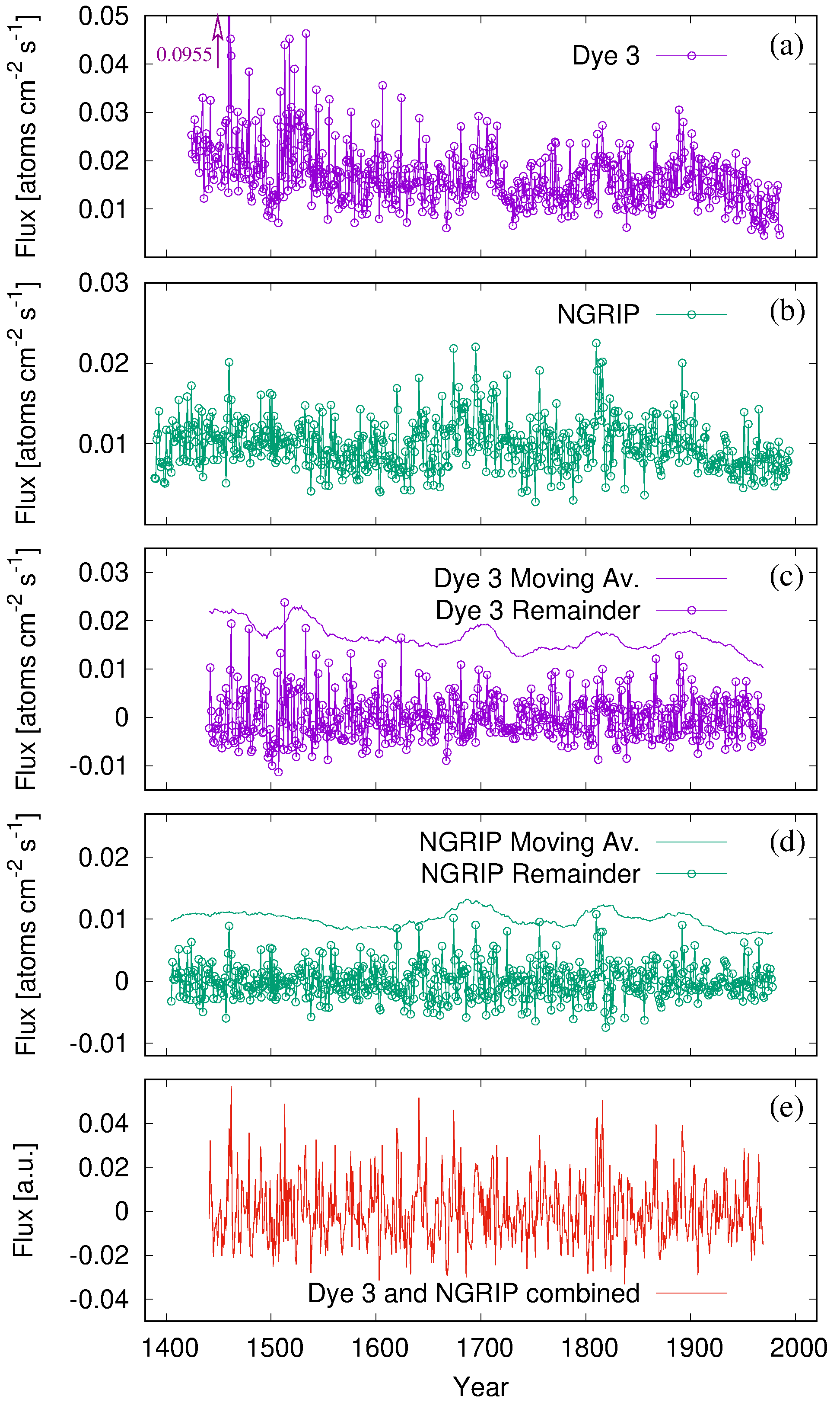
Figure 7: ¹⁰Be fluxes from Dye 3 (a), NGRIP (b), their individual moving averages and remainders (c,d), and their combined remainders (e).

The second data set comes from the NGRIP site (Berggren et al. 2009), originating from an ice core of 138 m depth, representing the time period A.D. 1389-1996.

Figure 7 reveals some systematic differences in the fluxes at both sites, which can be attributed to dilution effects due to different snow accumulation rates and/or other impacts on the ice core such as remelting, shear, drift of ice layers, etc..

For both data, Figures 7c and 7d show the split into a centered moving average (with 33 years), and the corresponding remainders, where the exceptionally strong peak for Dye 3 at A.D. 1460 has already been canceled and replaced by the average of the two neighboring data.

In order to average (as far as this makes any sense with only two samples) over noise and geographic peculiarities of the two sites, in Figure 7e we combine the remainders of Dye 3 and NGRIP, whereby the two individual contributions are weighted with the inverse of their standard deviation, in order to give them approximately equal weights.

4.3 Comparison of Schove’s data with radioisotope data

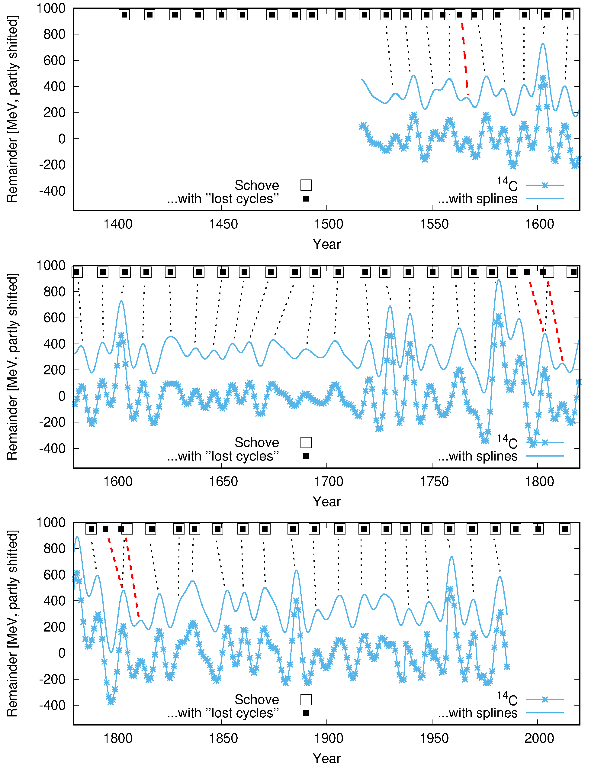
Figure 8: Schove’s maxima data, without (open squares) and with inclusion (full squares) of the “lost cycles”, the remainders of ¹⁴C, and a spline interpolation thereof (produced by gnuplot’s acsplines with a weight of 0.4). The black dotted lines connect the ¹⁴C maxima with the maxima of the (conventional) Schove data. The red dashed lines denote the complementary relationships for the “lost cycles”.

In Figures 8 and 9 we present Schove’s original maxima (open squares) and the modified series including “lost cycles” at 1563 (full squares), together with the remainders of the ¹⁴C and ¹⁰Be data, respectively, in three panels each covering an interval of 240 years (with some overlap). The ¹⁰Be data were also inverted in order to make their minima better identifiable with Schove’s maxima (the production rate of ¹⁰Be due to interaction of cosmic rays in the atmosphere is reciprocal to solar activity). The new maxima as derived from the radioisotopes by visual inspection are collected into the columns 4-7 of Table 1.

Despite some differences in detail, the maxima of the ¹⁴C series in Figure 8 seem to be well relatable to the corresponding maxima of Schove. A certain exception is the time of the Maunder minimum, in particular between 1650 and 1700, were the ¹⁴C maxima are systematically shifted to earlier times when compared with Schove’s maxima. Actually, this is in very good agreement with the open solar flux model of Owens et al. (2012) which shows that for weak solar cycles the relation between the sunspot number $R$ and the solar modulation potential $\Phi$ changes from in-phase to anti-phase. It remains to be seen whether the pronounced hemispherical character of the solar dynamo during the Maunder minimum (see Figure 6 in Ribes and Nesme-Ribes 1993) might play a complementary role in this respect.

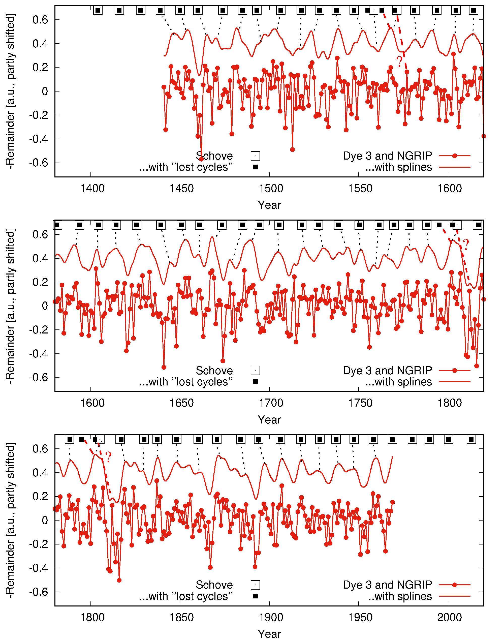
Figure 9: Schove’s maxima data, without (open squares) and with inclusion (full squares) of the “lost cycles”, inverted remainders of ¹⁰Be data, and a spline interpolation thereof (produced by gnuplot’s acsplines with a weight of 0.4). The black dotted lines connect the ¹⁰Be maxima with the maxima of the (conventional) Schove data. The red dashed lines denote the complementary relationships for the “lost cycles”.

What about the “lost cycles”? They are indicated by the dashed red lines in Figure 8, and given in the fifth column of Table 1. First, we can clearly identify an additional (weak) maximum at 1566, which seems relatable to Link’s additional maximum at 1563. In this sense, the ¹⁴C data would speak against Schove’s deliberate omittance of this cycle. As for Usoskin’s “lost cycle”, things are more complicated. The number of cycles indicated by the ¹⁴C data in the interval 1785-1820 signifies the emergence of one more maximum compared with Schove’s data. However, this additional maximum does not lay at 1795, as proposed by Usoskin (2002), but significantly later (at 1803). Similar time shifts apply also to the next two maxima (1812 vs 1805 and 1821 vs 1816). Things are even worse, since the weakest maximum, which we would expect to be close to Usoskin’s weak maximum at 1795, is actually found at 1812.

As a matter of fact, we find clear deviations between radionuclide data and Schove’s data in the interval 1785-1820, but without obvious systematics, so that for the moment this puzzle cannot be solved. We should keep in mind that the solar modulation potential in itself is a complicated functional of the solar magnetic field, whose topology might have changed during the “phase catastrophe” at the beginning of the Dalton minimum. In view of this uncertainty, we will continue with the consideration of both possible series of ¹⁴C maxima, without and with including both “lost cycles”, as summarized in the fourth and fifth column of Table 1.

Figure 9 shows the corresponding relationships for the ¹⁰Be data. Quite generally, these data are much more noisy than the ¹⁴C data, so that there is more ambiguity, first, in choosing a sensible smoothing parameter of the spline interpolation and, second, in relating the resulting maxima to Schove’s maxima. Hence, the choices made in Figure 9, and the resulting columns 6 and 7 in Table 1, should definitely be taken with a grain of salt. As for the Maunder minimum, we see that the shift to earlier times, as discussed for the ¹⁴C data, is also observable in the ¹⁰Be data, which gives further confidence in the corresponding model of Owens et al. (2012). The situation around 1565 (indicated by a question mark) with the first candidate of a “lost cycle” is quite peculiar. If we relate (one black dotted line) the clear ¹⁰Be maximum at 1567 with Schove’s maximum at 1571.3, we end up without any “lost cycle” at this point. Alternatively, we could relate the 1567 maximum with Link’s maximum at 1563, and the next (rather weak) ¹⁰Be maximum at 1577 (which is only visible in the remainder, but smeared out in the splines) with Schove’s maximum at 1571.3. With this second variant (indicated by two red dashed lines), we would include the “lost cycle” around 1565. A similar problem arises around 1800, although the qualitative behaviour of the ¹⁰Be data appears quite similar as the corresponding behaviour of ¹⁴C discussed above.

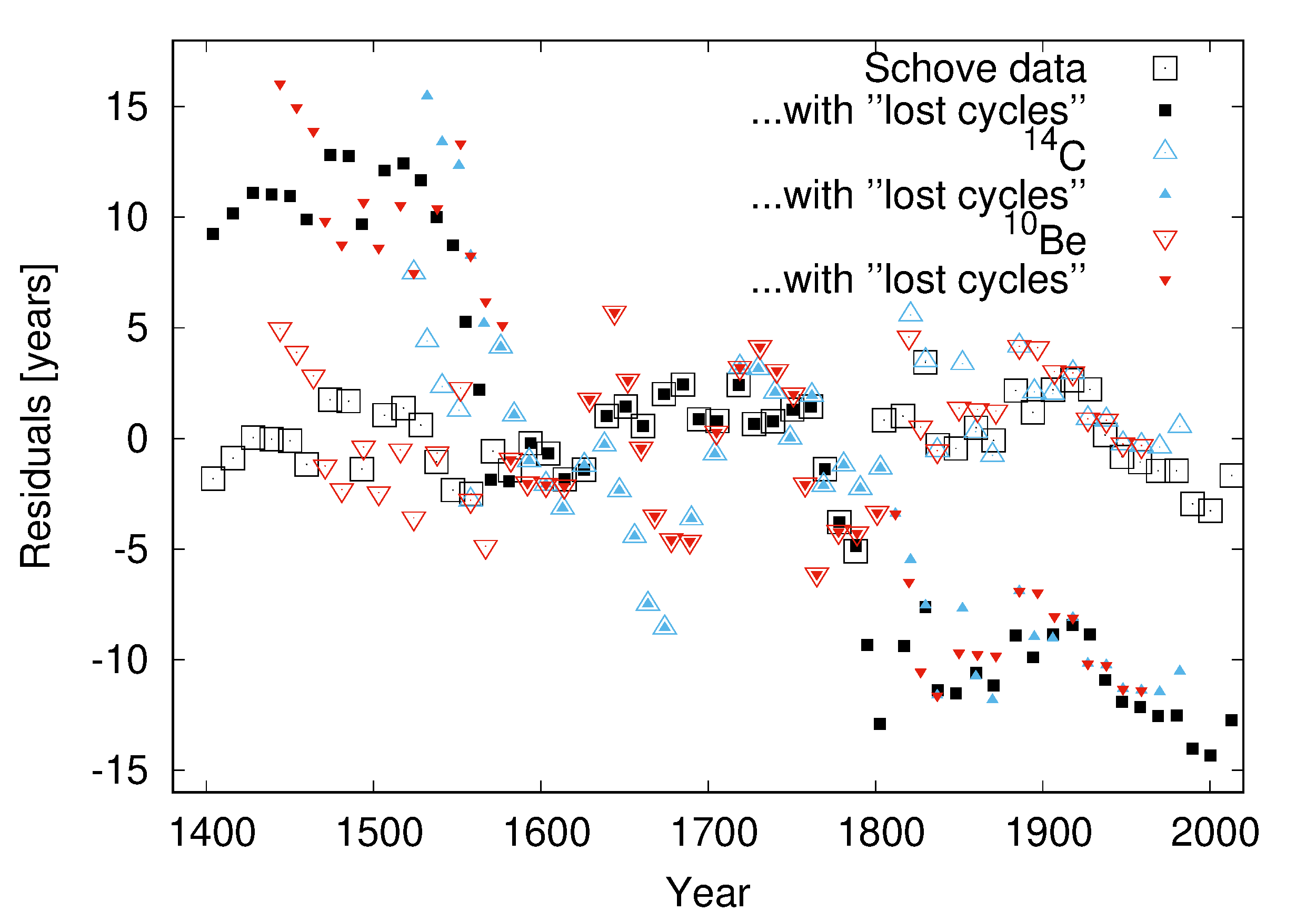
Figure 10: Residuals of Schove’s maxima data without and with inclusion of “lost cycles”, and of the corresponding maxima of the ¹⁴C and ¹⁰Be data.

In Figure 10 we illustrate all maxima data identified so far (for details see Table 1). Besides a re-plot (from Figure 3) of the two variants of Schove’s data we include now the maxima derived from ¹⁴C and ¹⁰Be, also in the two variants without or with the “lost cycles”. In general, we see reasonable agreement between the various data sets. The conspicuous “downswing” of both radioisotope data in the Maunder minimum interval 1650-1700 can consistently be explained by the phase-shift model of Owens et al (2012).

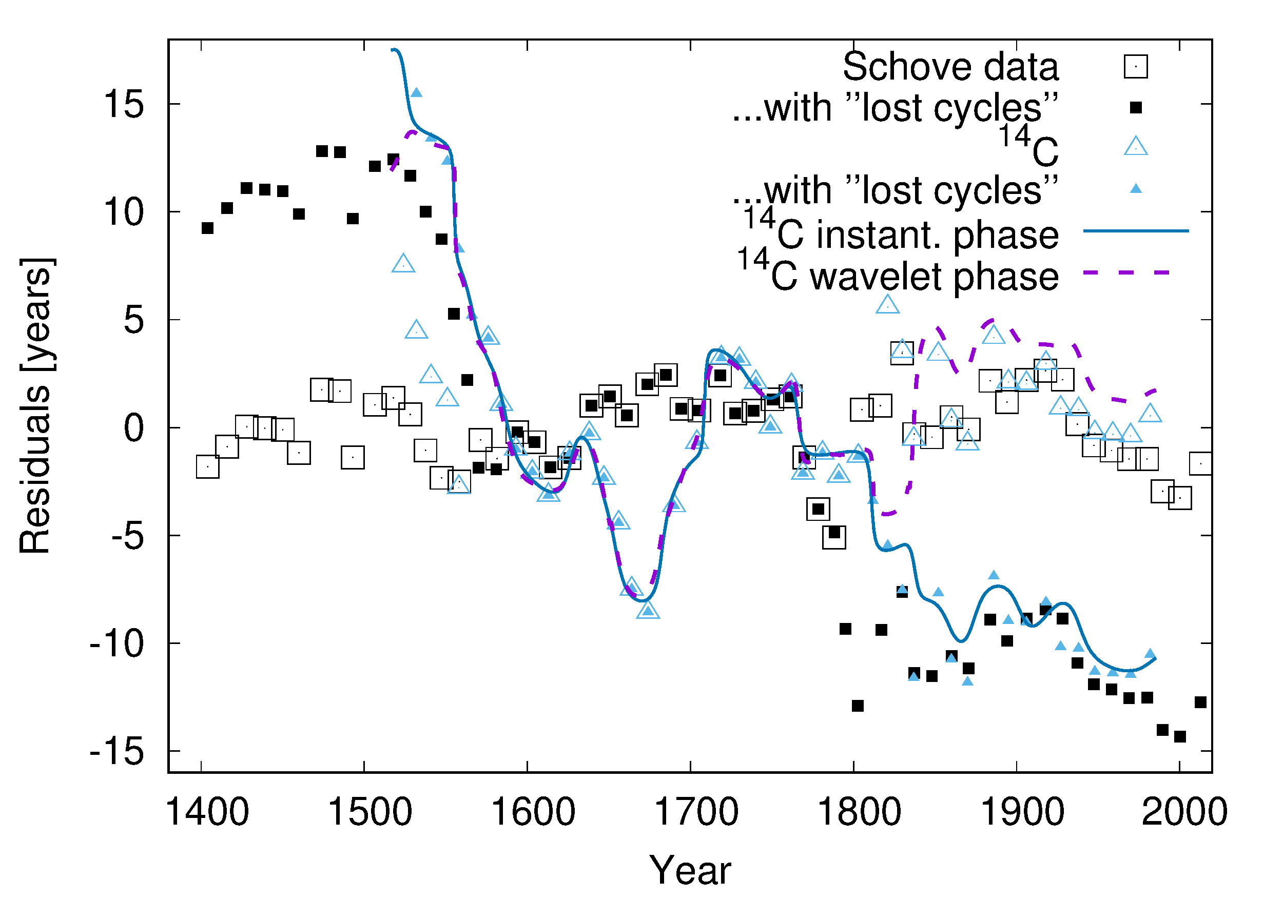
Figure 11: Residuals of Schove’s maxima without and with inclusion of “lost cycles”, and of the corresponding phase drifts (transformed into residuals) based on the instantaneous phase using a bandpass (between 17.85-year and 8-year periods) and a wavelet analysis. Note the divergence of the two phase drift curves after 1800.

Figure 11 is a modified version of Figure 10, with the less reliable ¹⁰Be maxima data omitted, but a deeper analysis of the ¹⁴C data. The residuals of their individual maxima are complemented by two continuous curves resulting from two types of phase drift computations. The first one (full line) is based on determining the instantaneous phase from band-passed data (Seilmeyer and Ratajczak 2017). The second one (dashed line) is based on a wavelet analyses (for details, see Appendix A). While both curves are nearly identical in the early segment of the data (where they cling to the maxima including Link’s “lost cycle”), they suddenly diverge after 1800. The curve based on the instantaneous phase continues according to the inclusion of Usoskin’s “lost cycle”, while the wavelet based curve jumps back to the ¹⁴C maxima data without “lost cycle”. Actually, the final results of both phase drift methods depend on details of their numerical implementation (width of the bandpass, wavelet parameter, etc.); at the critical points, where the amplitude of the 11.07-year oscillation drops significantly, they can either jump by one cycle or not. Loosely speaking, these sophisticated mathematical tools can complement, but not completely replace, the subjective decision (by visual inspection) on whether a (typically shallow) maximum should be counted as an additional cycle or not.

5 Conclusions

This paper was concerned with two types of phase jumps related to the solar cycle and its reflections in different proxy data. We started by highlighting the extremely important, but widely overlooked, results of Vos et al. (2004) which suggested, both for varved sediments from lake Holzmaar and for MSA distributions in the GISP2 ice core, an amazingly phase-coherent solar signal with a period of 11.04 years over the considered 1000 years period in the early Holocene. Then, we had a closer look into the “lost cycle” at the beginning of the Dalton minimum. While we remain rather indifferent with respect to it being real or not, in contrast to Usoskin (2002) we would interpret its existence - rather than its non-existence - as a “phase catastrophe”, or better, a phase jump within the otherwise synchronized Schwabe cycle with its 11.07 years periodicity. The same classification would apply to a similar “lost cycle” around 1565, which had been deliberately disregarded by Schove, despite some evidence in auroral data as pointed out by Link (1978). Finally, we have analyzed in some detail a series of ¹⁴C related data, and two series of ¹⁰Be data. After subtracting moving averages, the remainders of both data exhibit signals with a dominant 11 years periodicity, with the ¹⁴C data giving significantly clearer results. When comparing these data with Schove’s historical data we found - besides a reasonable agreement for most of the cycle maxima - some evidence for both Usoskin’s “lost cycle” around 1800 and for Link’s “lost cycle” around 1565. A careful re-analysis of the MSA distribution in the GISP2 ice core (Appendix A) suggests, in turn, that corresponding fast phase jumps in the early Holocene period might be not so strictly excluded as could be reasoned from the original work of Vos et al. (2004), who had used a comparably long observation window which suppresses short term events.

We would like to point out once more that the existence of phase jumps should in no way be considered a counter-argument against synchronization. To the contrary: their comparably sharp appearance within much longer phase-coherent intervals speaks even in favour of an underlying synchronization. However, as long as we have no sign information about the solar field during these times, there will always remain some ambiguity in attributing the (typically shallow) maximum to an additional full cycle (or not). Fortunately, this counting problem has only limited consequences, since the dynamo, having gone through this “nervous episode”, settles again into an ordered, synchronized state. Even the PSD of the cycle time series seems to be rather unaffected by those events, since the dominant cycle continues with the same phase relation.

Finally, we would like to discuss another interesting aspect of phase jumps. Regardless of their very existence (or not), Figure 3 exhibits a tendency for a systematic shortening of the Schwabe cycle approximately every 200 years. This mirrors the well-known Suess-de Vries cycle, which we had also confirmed in analyzing the spectrum of the residuals (Stefani et al. 2020). While much effort had been spent to explain this (and other) long-term cycle(s) in terms of corresponding periods of planetary tidal torques (Abreu et al. 2012), we pursued and extended the somewhat different idea of Cole (1973), Solheim (2013), Wilson (2013) that those long-term cycles may also arise as beat periods between significantly shorter cycles. Specifically, we enhanced our tidally synchronized solar dynamo model (which yields the 11.07-years Schwabe cycle) by a modulation of the field storage capacity of the tachocline with the period of the orbital angular momentum of the Sun which is dominated by the 19.86-year Jupiter-Saturn heliocentric conjunction period. This modulation of the 22.14-years Hale cycle provided a 193-year beat period of dynamo activity, which is indeed close to the Suess-de Vries cycle. With stronger 19.86-year forcing, we observed even additional Gleissberg-type periodicities around 100 years, which were intimately connected with the emergence of a Wilson gap, i.e. the prevalence of side bands around the 11.07-years cycle both at too short (e.g. 10 years) and too long (12 years) periods. The occurrence of such side bands can be explained by assuming that, intermittently, the shorter driving from spin-orbit coupling takes over and enslaves the mean Schwabe cycle to $19.86/2=9.93$ years, an effect which later must be compensated by one or a few longer cycles to “keep pace” with the basic 11.07-years tidal forcing cycle (which is still believed to be dominant). Yet, if the accumulated shortening of the residuals has become too extreme (see the -5 years residual around 1790 in Figure 3), then the next dynamo cycle might alternatively “slip back” by one tidal driving cycle. This would exactly correspond to the sort of phase jumps that we have been discussing in this paper.

While the long phase coherent period in the early Holocene together with the detailed analysis of the Schwabe cycle during the last 600 years has lend greater plausibility to our starting hypothesis of a tidally synchronized solar dynamo, we would like to encourage more investigations into the Schwabe cycle during other periods. Given the amazing quality of the varve thickness and MSA data as documented by Vos et al. (2004), it seems highly promising to investigate those data also for other periods in the Holocene.

Appendix A Computational methods: phase diagrams and wavelet analysis

In this appendix we present the numerical methods as they were used for producing the phase diagrams and for the wavelet analyses.

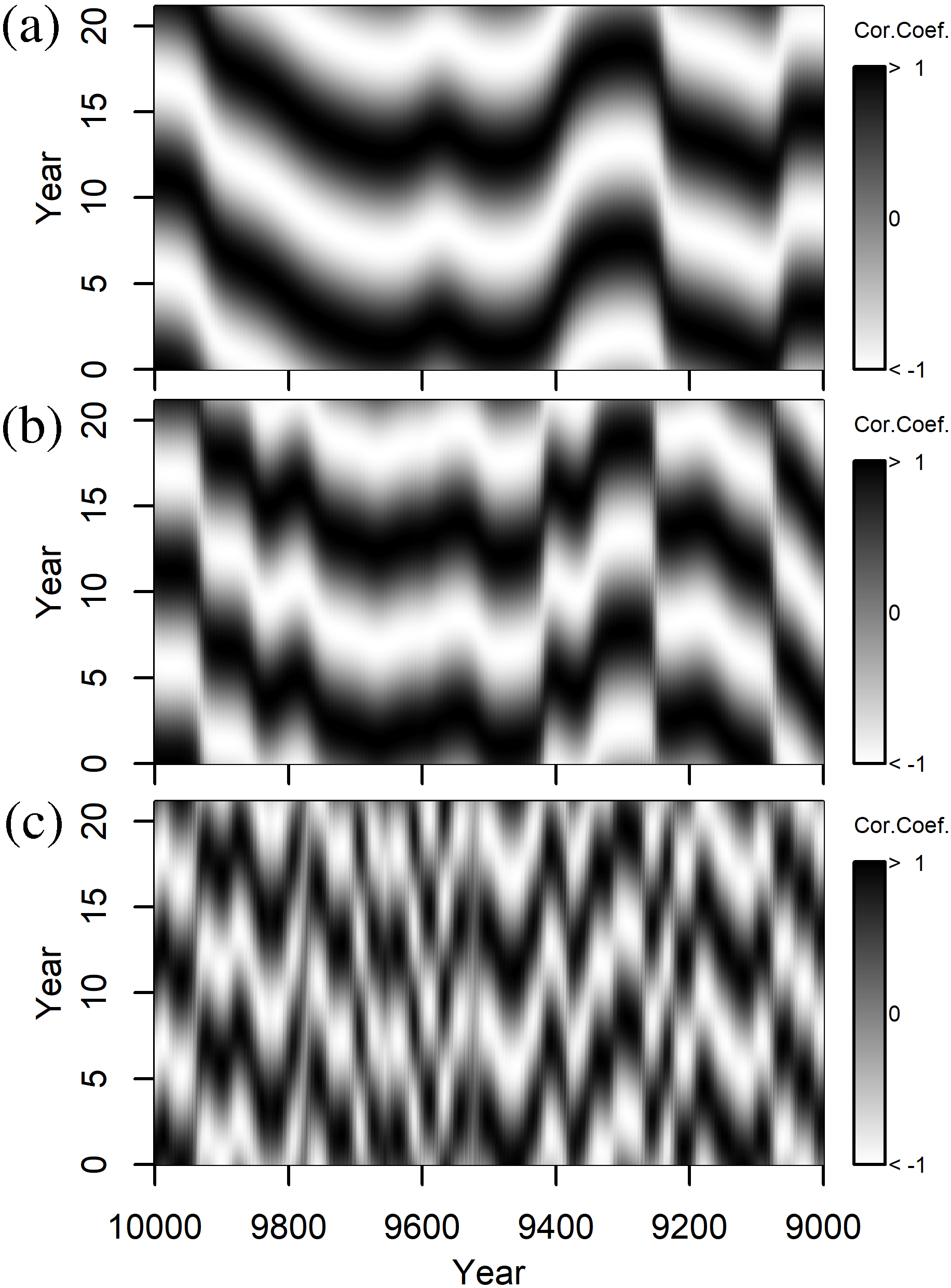
Figure 12: Phase diagrams of the MSA data from GISP2, as generated by means of the phaselet method with bandwidths $b=$(150 yr)^-1 (a), (85 yr)^-1 (b), (29 yr)^-1 (c). Not surprisingly, (b) yields a similar result as the method of Vos et al. (2004) with their rectangular time-domain window over 100 years, shown in Figure 1b. While the narrow bandwidth (a) gives a very smooth result, the wide bandwidth (c) suggests the occurrence of more transitions, which even might include real phase jumps by 11 years.

A.1 Phase diagrams

For the generation of the phase diagrams, we assume a time series to be given as an equally spaced interpolation on a regular grid. To these data we apply a band-pass filter, with a central frequency $f_{0}=$(11.07 yr)^-1, that consists of a weight function

$$w(f,f_{0},b)=\begin{cases}1-\left|\frac{f-f_{0}}{b}\right|^{3}&,\left|f-f_{0}\right|<b\\ 0&,\mathrm{else}\end{cases}$$ (1)

with cubic slope and bandwidth $b$. Given the Fourier transform of the signal to be

$$S(f)=\mathcal{F}(s(t))$$ (2)

the band pass filtered spectrum is defined as

$$S_{\mathrm{SP}}(f)=w(f,f_{0},b)\cdot S(f)$$ (3)

The shape of the bandpass filter in the frequency domain causes a specific shape of the observation window and vice versa. The selected cubic form corresponds to an overdamped sinc-like observation window including the main peak and only the first side peaks. Vos et al. (2004) introduced a rectangular window in time domain (ideal masking) which reflects an ideal sinc kernel in the frequency domain leading to undesired side bands. The latter bring about an unnecessarily wide observation window, which reduces the side bands but looses details in the resulting phase diagram. According to signal theory, the bandwidth is limited to $b<0.5f_{0}$ (violating this would lead to distortions due to aliasing). Note that an observation window of 100 years in time domain, as used by Vos et al. (2004), corresponds roughly to a bandwidth of $b\approx$(85 yr)^-1 in our case of a cubic frequency window.

Now we set up a function for the “phaselet”

$$\phi(t,\varphi,f_{0})=\begin{cases}\sin\left(2\pi f_{0}(\varphi+t)\right)&-1/f_{0}\leq\varphi<1/f_{0}\\ 0&\mathrm{else}\end{cases}$$ (4)

where $\varphi$ has the meaning of the shift (along the ordinate axis in the phase diagrams) and $t$ selects the time position in the data. The correlation is carried out in the usual way, so that the phaselet analysis

$$\mathcal{P}(t,\varphi,f_{0})=\int_{-1/f_{0}}^{1/f_{0}}s(t)^{*}\phi(t+t^{\prime},\varphi,f_{0})\thinspace\mathrm{dt^{\prime}}$$ (5)

can be given in form of the common correlation integral in the limits of $[-f_{0}^{-1},f_{0}^{-1}]$. Doing this for all $t$ and $\varphi$ results in the phase diagrams as presented in this paper.

As an example, we re-analyze with our method the MSA data from ice core GISP2 (Saltzmann et al. 1997) in order to compare the results with those of Vos et al. (2004), re-plotted here in Figure 1b. Figure A1 shows the resulting phase diagrams for a variety of bandwidths $b=$(150 yr)^-1 (a), (100 yr)^-1 (b), (85 yr)^-1 (c), and (50 yr)^-1 (d). While our result for $b=85$ (yr)^-1 corresponds approximately with Figure 1b, we can either get smoother results (for the narrow bandwidth (150 yr)^-1), or strongly fluctuating results (for the narrow bandwidth (50 yr)^-1).

A.2 Wavelet analysis

The spectral properties of a signal at a certain time can be conveniently revealed by wavelet analysis. The continuous wavelet transform of the real signal $f(t)$ is defined as

$$w_{f}(\tau,t)={\tau}^{-1}\int_{-\infty}^{\infty}f(t)\psi^{*}\left(\frac{t^{\prime}-t}{\tau}\right)\mathrm{dt^{\prime}},$$ (6)

where $\psi$ is the analyzing wavelet function, $\tau$ and $t$ define the scale (period of oscillation) and time, respectively. The specific choice of $\psi$ is always a compromise to balance resolution in time and scale. The popular Morlet wavelet

$$\psi(t)=e^{-t^{2}}\left(e^{2\pi it}-e^{-\pi^{2}}\right)$$ (7)

is used to satisfy the most of requirements for processing various records of solar activity (Frick et al. 2020). In addition to many widely used diagnostics we utilize wavelets here to perform the phase analysis. The phase drift between two oscillations with period $\tau$ in signals $f_{1}(t)$ and $f_{2}(t)$ evolves as

$$\delta\phi(t)=\arg(w_{1}(\tau,t)w_{2}^{*}(\tau,t)).$$ (8)

Figure 11 shows the residuals $-\tau\delta\phi(t)/(2\pi)$ with

$$w_{1}=\exp(2\pi i(t-66.75\cdot 11.07+1000)/11.07)$$ (9)

and $w_{2}=w_{{}^{14}C}(11.07,t)$. Also we added $\pm 2\pi$ appropriately to treat a discontinuity caused by the $\arg$-operation.

Appendix B Schove’s minima data and a waterfall diagram

In Table B1 we complement the maxima data from Table 1 by the corresponding minima data which were used for the generation of the Lomb-Scargle diagram in Figure 5. The restriction to the period 1500-2010 is due to the fact that Schove’s minima data before 1500 are not of the same reliability as the corresponding maxima data. The reason for that is that the most recent minima data in the Appendix of Schove (1983) were spoiled by wrong data between A.D. 511 - 1493: those were erroneously copied from the table of the corresponding maxima.

Table 2: Minima and maxima of solar cycles according to Schove (1983) and Hathaway (2015). The “lost cycles” as discussed by Link (1978) and Usoskin et al. (2002) are included in the columns “Li/Us”.

	Min		Max
SC	Schove	Li/Us	Schove	Li/Us
-22	1501.5		1506.5
-21	1513.7		1517.9
-20	1524.7		1528.2
-19	1534.3		1537.6
-18	1543.7		1547.4
-17	1554.5	1551.0	1558.3	1555
-16.5		1559.0		1563
-16	1567.5	1566.0	1571.3	1570
-15	1578.2	1576.0	1581.5	1581
-14	1587.5		1593.8
-13	1598.8		1604.4
-12	1609.2		1614.3
-11	1620.2		1625.8
-10	1633.7		1639.3
-9	1645.5		1650.8
-8	1655.9		1661.0
-7	1666.7		1673.5
-6	1679.5		1685.0
-5	1689.5		1694.5
-4	1699.0		1705.5
-3	1712.5		1718.2
-2	1723.5		1727.5
-1	1734.0		1738.7
0	1755.2		1750.3
1	1761.5		1761.5
2	1766.5		1769.75
3	1775.5		1778.42
4	1784.7	1784.3	1788.17	1788.4
4.5		1793.1		1795
5	1798.3	1799.8	1805.17	1802.5
6	1810.6	1810.8	1816.42	1817.1
7	1823.3		1829.92
8	1833.9		1837.25
9	1843.5		1848.17
10	1856.0		1860.17
11	1867.2		1870.67
12	1878.9		1884
13	1889.6		1894.08
14	1901.7		1906.17
15	1913.6		1917.67
16	1923.6		1928.33
17	1933.8		1937.33
18	1944.2		1947.42
19	1954.33		1958.25
20	1964.83		1968.92
21	1976.25		1980
22	1986.75		1989.58
23	1996.42		2000.33
24	2009.0		2013

Figure B1 complements the PSD data of Figure 5 by showing a “waterfall diagram”, or modified Gabor transform (Majkowski et al. 2014), of the combined maxima and minima data of Schove, supplemented by the two “lost cycles”. Besides the clear peak around 11 years, we observe also the typical shortening of the cycles before the “lost cycles”.

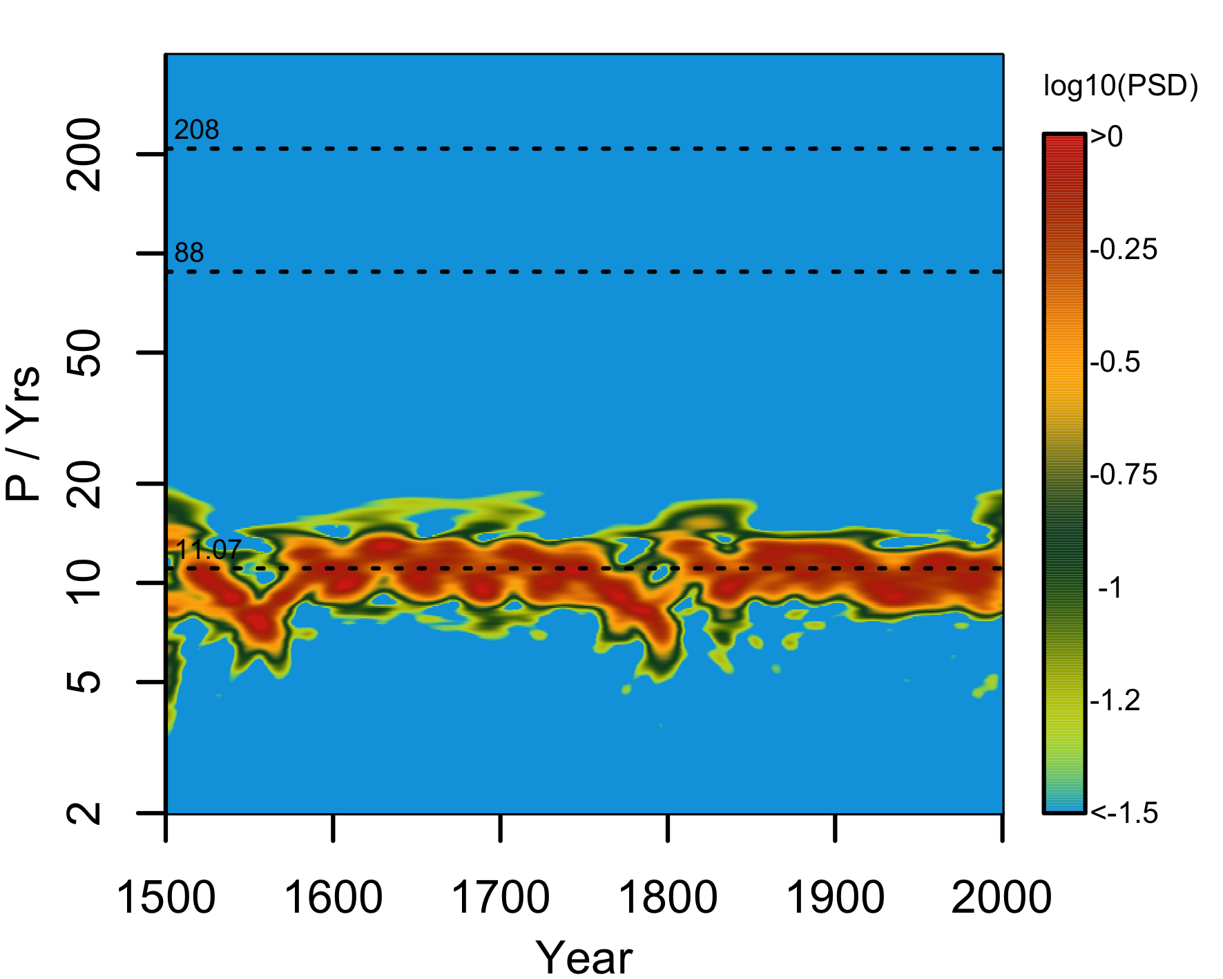
Figure 13: “Waterfall diagram” (modified Gabor transform) of Schove’s data with the two “lost cycles” included.

Appendix C Phase analysis, Lomb-Scargle diagram, and waterfall diagram for radioisotopes

In Figure C1 we show the phase diagrams for the ¹⁴C (a,b) and ¹⁰Be (c,d) data, produced by means of the phaselet method with bandwidths $b=$(85 yr)^-1 (a,c) and (29 yr)^-1 (b,d). Evidently, the resulting band structure is as far not as clear as in Figure 4. Given that the Schove/Hathaway data underlying Figure 4 should be considered as rather safe down to 1700, say, we tend to attribute the problem to the quality of the radioisotope data. From Figure C1d we also learn that for the recognition of the phase jump around 1565 an appropriately narrow observation window is recommendable, which might have consequences for the interpretation of missing phase jumps in Vos et al. (2004).

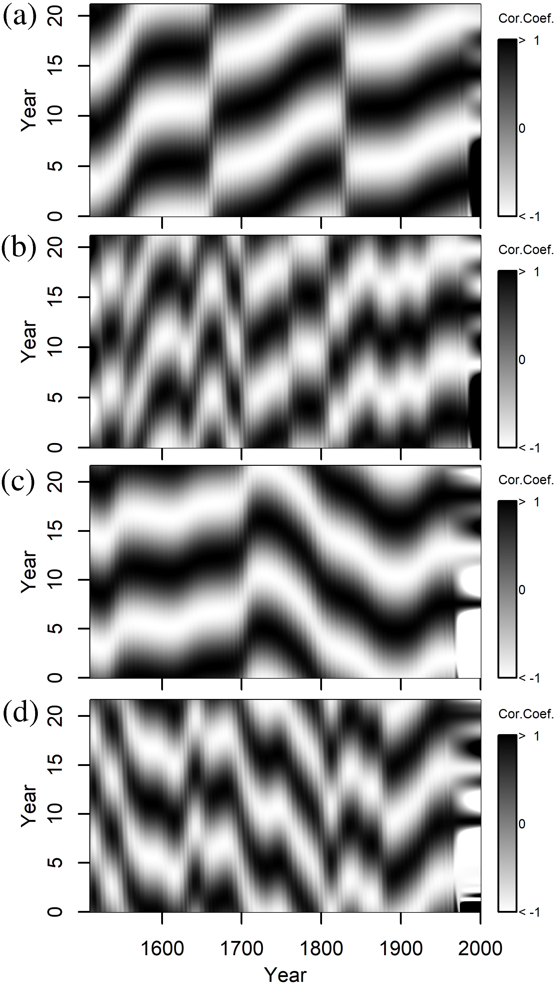
Figure 14: Phase diagrams of the radioisotope date: ¹⁴C (a,b) and ¹⁰Be (c,d), as generated by means of the phaselet method with bandwidths $b=$(85 yr)^-1 (a,c) and (29 yr)^-1 (b,d).

The corresponding Lomb-Scargle diagrams is shown in Figure C2, with a slightly shifted peak around 10.5 years, and another nice peak of the Suess-de Vries type (appr. 200 years). Additionally, Figure C3 shows the “waterfall diagram” (modified Gabor transform) of the ¹⁴C data.

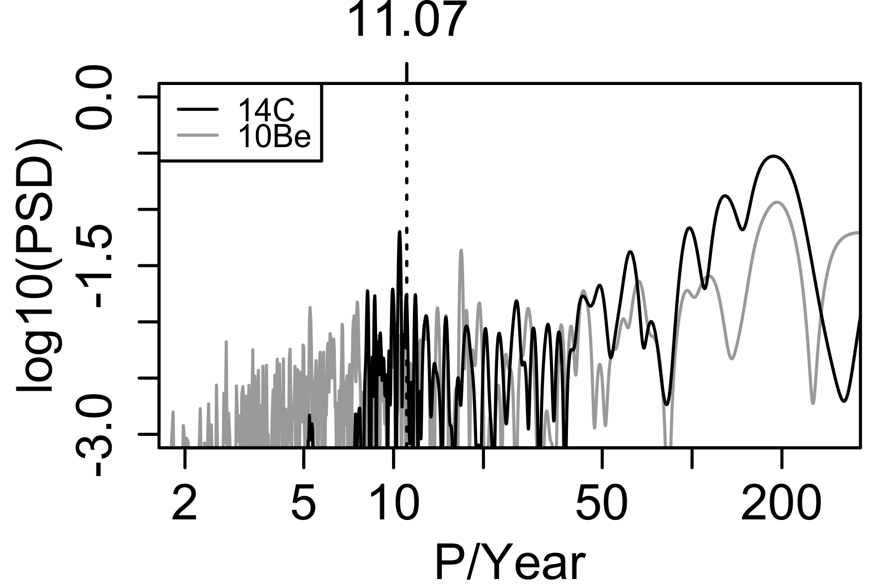
Figure 15: Lomb-Scargle diagram of the radioisotope date: ¹⁴C and ¹⁰Be.

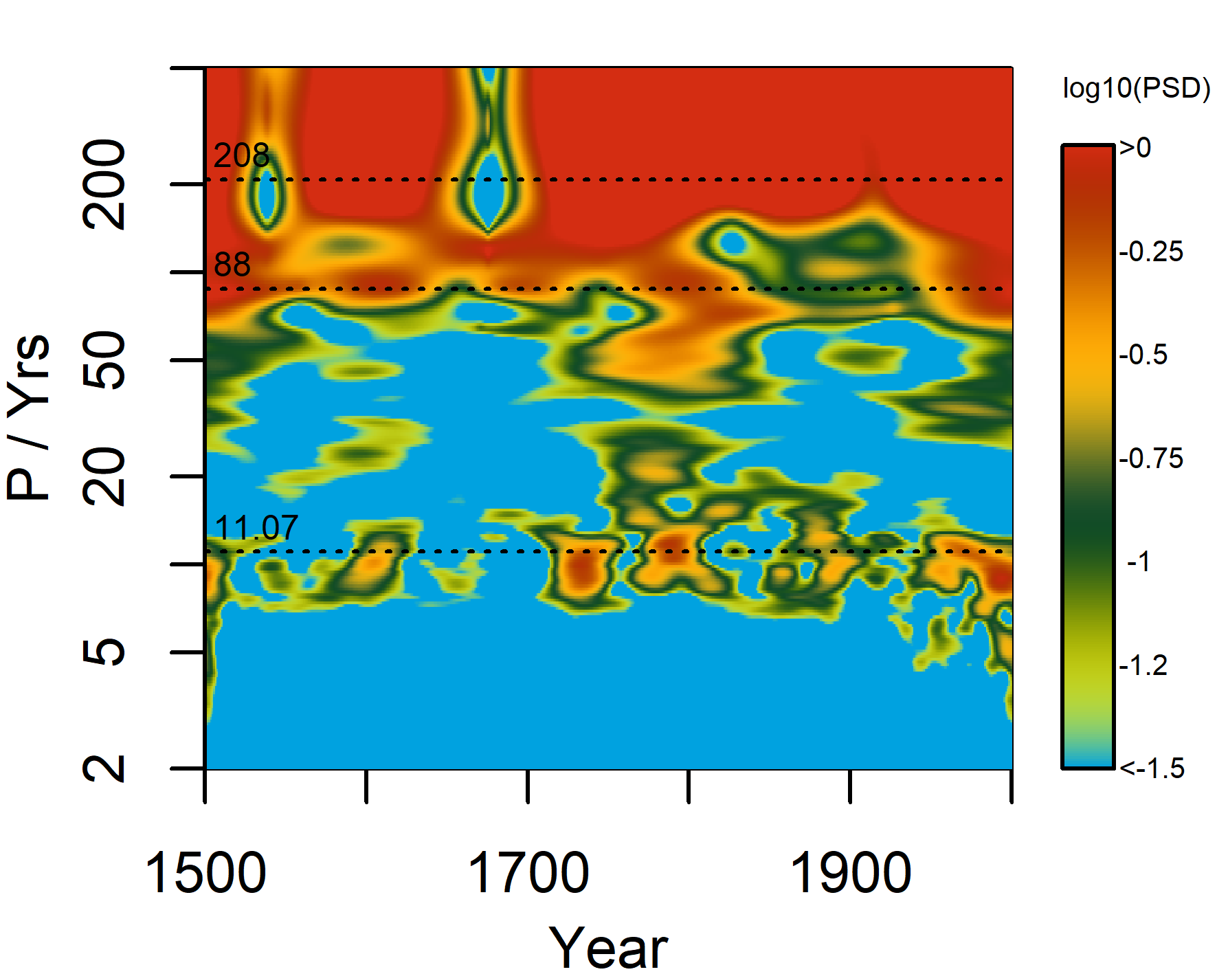
Figure 16: “Waterfall diagram” (modified Gabor transform) of the ¹⁴C data.