Margolus-Levitin speed limit across quantum to classical regimes based on trace distance

Abstract

The classical version of Mandelstam-Tamm speed limit based on the Wigner function in phase space is reported by B. Shanahan et al. [Phys. Rev. Lett. 120, 070401 (2018)]. In this paper, the Margolus-Levitin speed limit across the quantum-to-classical transition is given in phase space based on the trace distance. The Margolus-Levitin speed limit is set by the Schatten $L_{1}$ norm of the generator of time dependent evolution for both the quantum and classical domains. As an example, the time-dependent harmonic oscillator is considered to illustrate the result.

Keywords: Quantum speed limit; Wigner function; Phase space; Margolus-Levitin bound

PACS: 03.65.-w; 03.65.Db; 03.67.-a

I Introduction

The notion of quantum speed limit (QSL) was proposed by Mandelstam and Tamm Mandelstam45 in 1945. The Mandelstam-Tamm (MT) bound of QSL, which is defined by the variance of the energy $\frac{\pi\hbar}{2\Delta E}$, can be considered as the extension of the Heisenberg time-energy relation. Later, Margolus and Levitin Margolus98 ; Levitin09 found another bound form of QSL (ML bound), which is based on the mean energy $\frac{\pi\hbar}{2(\langle E\rangle-E_{0})}$. The ML bound can be considered as the transition probability amplitude between two orthogonal quantum states $\langle\psi_{0}|\psi_{\tau}\rangle$. In order to get the tight bound, the unified QSL is defined by the larger one between the MT and ML bound, i.e., $\tau_{\text{qsl}}=\max\left\{\frac{\pi\hbar}{2\Delta E},\frac{\pi\hbar}{2(\langle E\rangle-E_{0})}\right\}$.

The investigation of QSL can deepen the understanding of time-energy uncertainty relation, the quantum evolution, the quantum control Caneva09 , even the information of black hole Bekenstein81 . In particular, the QSL has been investigated in different methods for the closed systems Fleming73 ; Bhattacharyya83 ; Anandan90 ; Pati91 ; Vaidman92 ; Brody03 ; Jones10 ; Campaioli18 , and extended to the open systems recently Taddei13 ; Campo13 ; Deffner13 ; Xu14 ; Zhang14 ; Sun15 ; Jing16 ; Pires16 ; Wu15 ; Wu18 ; Cai17 ; Zhang16 ; Yu18 ; He16 ; Liu19 ; Teittinen19 ; Funo19 ; Hou17 ; Xu19 ; Zhang18 ; Mondal16 ; Sun19 ; Haseli19 ; Deffnernjp ; Xu18 ; Pintos19 ; Campbell17 ; Xu14cpl ; Feng19 ; Wang20 . One can also see the comprehensive review article Deffner17 . According to Bohr’s correspondence principle, the effect of the reduced Planck’s constant $\hbar$ will vanish gradually when the system transitions to the classical world from quantum scale. So, it will cause both the ML and the MT bounds of QSL to become zero,

$$\lim_{\hbar\rightarrow 0}\tau_{\text{qsl}}=0.$$ (1)

Considering the quantum speed limit originated from the Heisenberg time-energy uncertainty relationship, people are usually made to believe that the quantum speed limit is the unique phenomenon of quantum mechanics. However, the speed limit for classical dynamics, unrelated with the quantum/classical nature, were reported by B. Shanahan et al. Shanahan18 and M. Okuyama et al. Okuyama18 , independently. Using the fidelity and employing the Cauchy-Schwarz inequality, B. Shanahan et al. obtained a MT bound of speed limit based on the quasiprobability distributions in the Wigner function, which can describe the transition across the quantum to classical regime in phase space. From the quantum-to-classical domain, the speed of evolution is determined by the Schatten $L_{2}$ norm of Moyal bracket for the Hamiltonian, the Wigner function and the Bhattacharyya coefficient, respectively. A natural question is whether there also exists a ML bound for the classical speed limit.

In this paper, we derive the Margolus-Levitin bound for speed limit of classical system in phase space based on trace distance. The ML bound for the speed limit across the quantum-to-classical transition can be obtained through the triangle inequality for integral, and it is governed by the Schatten $L_{1}$ norm of time dependent evolution generator for both the quantum and classical regimes. As an example, the time-dependent harmonic oscillator is given to illustrate the result. The distinction between the Margolus-Levitin bound in this paper and the Mandelstam-Tamm bound in Ref. Shanahan18 are discussed. This paper is organized as follows. In Sec. II, we give the definition of Margolus-Levitin quantum speed limit in phase space. In Sec. III, the ML semiclassical speed limit is defined. In Sec. IV, the ML classical speed limit is obtained, and an example is given. The discussion and the conclusion are given in the end.

II The Margolus-Levitin quantum speed limit in phase space

Motivated by Ref. Shanahan18 , we will derive the ML bound of speed limit in phase space representation. The Wigner function of one-dimensional system $\rho_{t}$ is defined as Hillery84 ; Zachos05

$$W_{t}(q,p)=\frac{1}{\pi\hbar}\int\langle q-y|{\rho}_{t}|q+y\rangle e^{-2ipy/\hbar}dy,$$ (2)

where $q,p$ are the generalized coordinate and momentum respectively, and $\langle q|{\rho}_{t}|q^{\prime}\rangle$ is the density matrix in the coordinate representation. In the following paper, we will consider the unitary dynamics of pure state under the time dependent Hamiltonian ${H}$, and the “distance” measure between the initial state and final state is chosen as the trace distance, which is given by

$$\mathcal{T}(\rho_{t},\rho_{0})=\text{Tr}|\rho_{t}-\rho_{0}|=\|\rho_{t}-\rho_{0}\|_{1}.$$ (3)

Turning into the Wigner phase space, the distance $\mathcal{T}(W_{t},W_{0})$ between the pure initial state with Wigner function $W_{0}$ and the time-dependent final state with Wigner function $W_{t}$ is Deffnernjp

$$\mathcal{T}(W_{t},W_{0})=\int d^{2}\Gamma|W_{t}-W_{0}|,$$ (4)

where $d^{2}\Gamma=2\pi\hbar dqdp$.

In order to consider the time-dependent change rate of the trace distance, the motion of Wigner function $W_{t}$ can be expressed by the Moyal bracket Zachos05

$$\frac{\partial W_{t}}{\partial t}=\{\{H,W_{t}\}\}=\frac{1}{i\hbar}(H_{qp}\star W_{t}-W_{t}\star H_{qp}),$$ (5)

where $\{\{H,W_{t}\}\}$ is the Moyal bracket and $\star$-product means the Moyal product $H_{qp}\star W_{t}=H_{qp}\text{exp}\Big{(}\frac{i\hbar}{2}\overleftarrow{\partial_{q}}\overrightarrow{\partial_{p}}-\frac{i\hbar}{2}\overleftarrow{\partial_{p}}\overrightarrow{\partial_{q}}\Big{)}W_{t}(q,p)$ with Weyl ordered Hamiltonian operator $H_{qp}=\int dx\langle q-x/2|H|q+x/2\rangle\exp(ipx/\hbar)$. Similar to Refs. Deffnernjp ; Cai17 , the rate of change for the trace distance $\mathcal{T}(W_{t},W_{0})$ can be derived as

$$\dot{\mathcal{T}}(W_{t},W_{0})=\int d^{2}\Gamma\frac{W_{t}-W_{0}}{|W_{t}-W_{0}|}\{\{H,W_{t}\}\}.$$ (6)

Using the property of integral (or the triangle inequality for integral), it can lead to the following inequality:

$$\dot{\mathcal{T}}(W_{t},W_{0})\leq|\dot{\mathcal{T}}(W_{t},W_{0})|\leq\int d^{2}\Gamma|\{\{H,W_{t}\}\}|.$$ (7)

It should be note that the value of $(W_{t}-W_{0})/|W_{t}-W_{0}|$ is $\pm 1$. And, it is easy to obtain that

$$\int d^{2}\Gamma|\{\{H,W_{t}\}\}| =\int d^{2}\Gamma\left|\frac{\partial W_{t}}{\partial t}\right|$$

$$=\int 2\pi dqdp\langle q-y|(|\dot{\rho}_{t}|)|q+y\rangle\langle q+y^{\prime}|\mathbb{I}|q-y^{\prime}\rangle e^{2ip(y^{\prime}-y)/\hbar}dydy^{\prime}$$

$$=2\int dqdy\langle q-y|(|\dot{\rho}_{t}|)|q+y\rangle\langle q+y|\mathbb{I}|q-y\rangle$$

$$=2\int\frac{dXdY}{2}\langle X|(|\dot{\rho}_{t}|)|Y\rangle\langle Y|X\rangle$$

$$=\text{Tr}|\dot{\rho}_{t}|,$$ (8)

where $\mathbb{I}$ means the identical density matrix. Substituting the Heisenberg equation $i\hbar{\partial_{t}{\rho}_{t}}=[H,\rho_{t}]$ into Eq. (8), we can get the following inequality:

$$\text{Tr}|\dot{\rho}_{t}| =\frac{1}{\hbar}\text{Tr}|[\rho_{t},H]|$$

$$\leq\frac{1}{\hbar}\text{Tr}|\rho_{t}H|+\frac{1}{\hbar}\text{Tr}|H\rho_{t}|.$$ (9)

In the second line, the triangle inequality for trace norm is used. For the normalized pure state, we can obtain that

$$\text{Tr}|\rho_{t}H|=\text{Tr}\sqrt{H|\psi_{t}\rangle\langle\psi_{t}|H}=\langle H\rangle,$$ (10)

where $\langle H\rangle$ is the mean energy. Without loss of generality, following Ref. Margolus98 , assuming that the system has discrete spectrums, and the energy eigenvalues $\{E_{n}\}$ associated with the eigenstates $\{|E_{n}\rangle\}$ are in ascending order. When choosing the energy of ground state properly and assuming that the value of ground state $E_{0}$ is zero, we can have

$$\text{Tr}|\rho_{t}H|=\langle H\rangle-E_{0}$$ (11)

Combining the above Eqs. (6-11), we arrive at

$$|\dot{\mathcal{T}}(W_{t},W_{0})|\leq\int d^{2}\Gamma|\{\{H,W_{t}\}\}|\leq\frac{2(\langle H\rangle-E_{0})}{\hbar}.$$ (12)

Integrating Eq. (12) over time from $0$ to $\tau$, we can obtain that

$$\tau\geq\frac{\hbar\mathcal{T}(W_{\tau},W_{0})}{2E_{\tau}}\geq\frac{\mathcal{T}(W_{\tau},W_{0})}{\langle v_{\text{qsl}}\rangle},$$ (13)

where

$$E_{\tau}=(1/\tau)\int_{0}^{\tau}dt(\langle H\rangle-E_{0})$$ (14)

is the time-averaged energy, and

$$\langle v_{\text{qsl}}\rangle=(1/{\tau})\int_{0}^{\tau}dt\|\{\{H,W_{t}\}\}\|_{1}$$ (15)

is defined as the time-averaged velocity in the quantum information processing. The Schatten $L_{1}$ norm of Moyal bracket

$$\|\{\{H,W_{t}\}\}\|_{1}=\int d^{2}\Gamma|\{\{H,W_{t}\}\}|=v_{\text{qsl}}$$ (16)

can be considered as the instantaneous velocity of quantum state evolution in phase space. Eq. (13) has the same form as the original Margolus-Levitin speed limit $\frac{\hbar\pi}{2(\langle E\rangle-E_{0})}$ and is related to the value of time-averaged energy, so it can be considered as Margolus-Levitin quantum speed limit bound in phase space

$$\tau\geq\tau_{\text{qsl}}=\frac{\mathcal{T}(W_{\tau},W_{0})}{(1/{\tau})\int_{0}^{\tau}dt\|\{\{H,W_{t}\}\}\|_{1}},$$ (17)

which is governed by the Schatten $L_{1}$ norm of Moyal bracket.

III The Margolus-Levitin semiclassical speed limit

The Moyal bracket can be expanded through Taylor expansion in term of $\hbar$, and will be reduced to the Poisson bracket when ignoring the higher-order terms. It can be expressed as follows Zachos05

$$\{\{H,W_{t}\}\}=\{H,W_{t}\}+\mathcal{O}(\hbar^{2}).$$ (18)

The Poisson bracket is defined as functions of the partial derivatives of generalized canonical coordinate $q$ and momentum $p$, i.e.,

$$\{f,H\}=\frac{\partial H}{\partial p}\frac{\partial f}{\partial q}-\frac{\partial H}{\partial q}\frac{\partial f}{\partial p},$$ (19)

and it governs the dynamics of classical mechanics.

Due to the Wigner function containing the reduced Planck’s constant $\hbar$, the semiclassical speed limit (SSL) can also be given based on the Poisson bracket as

$$\tau\geq\tau_{\text{ssl}} =\frac{\mathcal{T}(W_{\tau},W_{0})}{\langle v_{\text{ssl}}\rangle},$$ (20)

where,

$$\langle v_{\text{ssl}}\rangle=(1/{\tau})\int_{0}^{\tau}dt\|\{H,W_{t}\}\|_{1}$$ (21)

is the time-averaged velocity of system evolution governed by the Poisson bracket. The upper bound of the instantaneous evolution velocity is defined by the absolute value for the change rate of Wigner function averaged over the phase space, i.e.,

$$v_{\text{ssl}} =\int d^{2}\Gamma|\partial_{t}W_{t}|=\int d^{2}\Gamma|\{H,W_{t}\}|$$

$$=\|\{H,W_{t}\}\|_{1}.$$ (22)

In order to derive the formula (20), one only need to replace the Moyal bracket $\{\{H,W_{t}\}\}$ by the Poisson bracket $\{H,W_{t}\}$. Because the Wigner function $W_{t}$ contains the reduced Planck’s constant $\hbar$, it is appropriate to say that Eq. (20) is a Margolus-Levitin semiclassical speed limit (ML-SSL) bound. Independent of the quantum approach, Eq. (20) can also been derived through the classical mechanics. The Hamilton’s equation of motion in classical mechanics is

$$\frac{\partial W_{t}}{\partial t}=\{H,W_{t}\},$$ (23)

so the semiclassical speed limit can be arrived straightforwardly

$$\tau\geq\tau_{\text{ssl}}=\frac{\mathcal{T}(W_{\tau},W_{0})}{(1/\tau)\int_{0}^{\tau}dt\|\hat{L}W_{t}\|_{1}}.$$ (24)

The Liouvillian $i\hat{L}W_{t}=-\{H,W_{t}\}$ is introduced in Eq. (24). Similar to Eq. (17) in the quantum case, the ML-SSL is also set by the Schatten $L_{1}$ norm of Liouvillian $\hat{L}$. It should be noticed that the expression ML-SSL in phase space is dependent on the Winger function, and still includes the reduced Planck’s constant $\hbar$.

IV The Margolus-Levitin classical speed limit

Now, we will derive the speed limit for the classical evolution. According to the operational dynamic modeling Bondar12 ; Bondar13 , the relationship for the evolution of the dynamical average values between the classical phase-space probability density $\varrho_{t}(q,p)$ and the Wigner function $W_{t}(q,p)$ can be connected through the Ehrenfest theorems, which is given by

$$\varrho_{t}(q,p)=2\pi\hbar W_{t}(q,p)^{2}.$$ (25)

For a pure state $|\psi\rangle$, the normalized condition meets $2\pi\hbar\int dqdpW_{t}(q,p)^{2}=\int dqdp\varrho_{t}(q,p)=1$. Similar to the original seminal work of Margolus-Levitin quantum speed limit bound derived from the transition probability amplitude between two orthogonal states $\langle\psi_{0}|\psi_{t}\rangle$, the overlap between states $\varrho_{0}$ and $\varrho_{t}$ can be re-expressed by the Bhattacharyya coefficient Bhattacharyya46

$$B(\varrho_{t},\varrho_{0})=\int dqdp\sqrt{\varrho_{0}\varrho_{t}}.$$ (26)

Reminiscing the Hellinger distance $H(\varrho_{t},\varrho_{0})^{2}=\frac{1}{2}\text{Tr}[(\sqrt{\varrho_{0}}-\sqrt{\varrho_{t}})^{2}]$, which can be used to measure the quantum correlation Wu14 ; Chang13 ; Girolami13 , it is easy to verify that $B(\varrho_{t},\varrho_{0})=1-H(\varrho_{t},\varrho_{0})^{2}.$

The trace distance between the initial and final states can be expressed as

$$\mathcal{T}(\varrho_{t},\varrho_{0})=\int dqdp|\sqrt{\varrho_{t}}-\sqrt{\varrho_{0}}|,$$ (27)

and the classical speed limit can be derived straightforwardly as

$$\tau\geq\tau_{\text{csl}} =\frac{\mathcal{T}(\varrho_{\tau},\varrho_{0})}{\langle v_{\text{csl}}\rangle},$$ (28)

where,

$$\langle v_{\text{csl}}\rangle=(1/{\tau})\int_{0}^{\tau}dt\|\{H,\sqrt{\varrho_{t}}\}\|_{1}$$ (29)

is the time-averaged velocity of classical system dynamics. The instantaneous classical evolution velocity is defined as the Schatten $L_{1}$ norm of $\{H,\sqrt{\varrho_{t}}\}$

$$v_{\text{csl}} =\|\{H,\sqrt{\varrho_{t}}\}\|_{1}=\int dqdp\left|\{H,\sqrt{\varrho_{t}}\}\right|$$

$$=\int dqdp|\partial_{t}\sqrt{\varrho_{t}}|.$$ (30)

Eq. (28) is a classical version of Margolus-Levitin speed limit bound for system evolution, and it can be obtained using only the classical approach. The classical Liouville operator satisfies $\partial_{t}\varrho_{t}+i\hat{L}\varrho_{t}=0$, so the derivative of trace distance is

$$\dot{\mathcal{T}}(\varrho_{t},\varrho_{0}) \leq|\dot{\mathcal{T}}(\varrho_{t},\varrho_{0})|$$

$$=\int dqdp|\hat{L}\sqrt{\varrho_{t}}|=\|\hat{L}\sqrt{\varrho_{t}}\|_{1}.$$ (31)

Integrating Eq. (31) over time from $0$ to $\tau$, we can obtain that

$$\tau\geq\tau_{\text{csl}}=\frac{\mathcal{T}(\varrho_{\tau},\varrho_{0})}{(1/\tau)\int_{0}^{\tau}dt\|\hat{L}\sqrt{\varrho_{t}}\|_{1}}.$$ (32)

This is the main result of this paper, and it is a classical Margolus-Levitin version bound of speed limit for classical dynamics.

Similar to Ref. Shanahan18 , we would like to consider the time-dependent harmonic oscillator as an example to illustrate the above results. The time-dependent harmonic oscillator can be applied to the control protocols Campbell17 ; Chen10 , the quantum thermal machines Campo14 , etc. The Hamiltonian is given by

$$\hat{H}=\frac{{p}^{2}}{2m}+\frac{1}{2}m\omega(t)^{2}{q}^{2}.$$ (33)

In the quantum case, the Wigner function of state under the modulation of trapping frequency $\omega(t)$ is

$$W_{n}(q,p;t)= W_{n}(Q,P;0)$$

$$= \frac{(-1)^{n}}{\pi\hbar}e^{-(2/\hbar\omega_{0})[P^{2}/(2m)+(1/2)m\omega_{0}^{2}Q^{2}]}$$

$$\times L_{n}\Big{[}\frac{4}{\hbar\omega_{0}}\Big{(}\frac{P^{2}}{2m}+\frac{1}{2}m\omega_{0}^{2}Q^{2}\Big{)}\Big{]},$$ (34)

where $L_{n}[x]$ is the Laguerre polynomials and $Q=q/b$, $P=bp-mq\dot{b}$ are the pairs of canonically conjugated variables, respectively. The time-dependent factor $b(t)$ is governed by the Ermakov equation $\ddot{b}+\omega(t)^{2}b=\omega_{0}^{2}/b^{3}$, where the boundary conditions are $b(0)=1$ and $\dot{b}(0)=0$ Chen10 ; Chen10prl .

Suppose that the initial ground state of harmonic oscillator with $n=0$, and $W_{0}(q,p,t)\geq 0$ is a smooth Gaussian distribution for all $0\leq t\leq\tau$. The classical distribution is chosen as the Gaussian form $\varrho_{0}(q,p)=\exp(-q^{2}/\sigma_{q}^{2}-p^{2}/\sigma_{p}^{2})/(\pi\sigma_{q}\sigma_{p})$ and $\sigma_{q}=x_{0}/\sqrt{2}$, $\sigma_{p}=\hbar/(x_{0}\sqrt{2})$. The state $\varrho_{t}(q,p)$ can be evaluated by $\varrho_{t}(q,p)=\varrho_{0}(Q,P)$, and the Bhattacharyya coefficient can be calculated analytically as

$$B(\varrho_{0},\varrho_{t})=2\Big{[}\frac{(1+b^{2})^{2}}{b^{2}}+\Big{(}\frac{m\sigma_{q}\dot{b}}{\sigma_{p}}\Big{)}^{2}\Big{]}^{-1/2}.$$ (35)

The upper Margolus-Levitin bound of evolution instantaneous velocity in phase space is

$$v_{\text{csl}}=\|H,\sqrt{\varrho_{t}}\|_{1}=\sqrt{\frac{\sigma_{q}}{\pi\sigma_{p}}}4m\sigma_{q}|\ddot{b}(t)|.$$ (36)

The driven Hamiltonian is assumed to be a constant for $t>0$, and the frequency of trapping turns off suddenly at $t=0$. One can find that $b(t)=\sqrt{1+\omega_{0}^{2}t^{2}}$ and $\ddot{b}(t)=\omega_{0}^{2}$. In Fig. 1, we show the Margolus-Levitin velocity $v_{\text{csl}}$ in phase space, the Mandelstam-Tamm velocity $v_{\Gamma}^{\text{CSL}}$ reported in Ref. Shanahan18 and the absolute value of the Bhattacharyya coefficient derivative $|\dot{B}(\varrho_{0},\varrho_{t})|$ during the evolution, respectively. What needs illustration is that the Margolus-Levitin speed limit (32) can not be compared with the Mandelstam-Tamm speed limit in Ref. Shanahan18 , because the original “distance” measures of them are different.

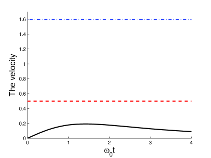
Figure 1: Classical speed limit of evolution in phase space. The black solid line is the absolute value of the Bhattacharyya coefficient derivative $|\dot{B}(\varrho_{0},\varrho_{t})|$; The red dashed line is the Mandelstam-Tamm upper bound of speed $v_{\Gamma}^{\text{CSL}}$ reported in Ref. Shanahan18 ; The blue dot-dashed line is the Margolus-Levitin upper bound of instantaneous speed $v_{\text{csl}}$ in Eq. (36). The unit of time is set by $\omega_{0}^{-1}$.

V Discussion and conclusion

In this paper, we obtained the Margolus-Levitin speed limit across the quantum to classical regime based on the trace distance. However, the trace distance is not a bona fide measure to derive the Mandelstam-Tamm speed limit in phase space, because the Cauchy-Schwarz inequality for $n\times n$-dimensional matrix, i.e., $|\text{Tr}A|\leq\sqrt{n}\sqrt{\text{Tr}(A^{{\dagger}}A)}$, can not be extended to infinite dimension system directly. In addition, to the best of our knowledge, since the von Neumann inequality can only be applied to matrices, the fidelity or the overlap between states, which can lead to the Mandelstam-Tamm speed limit in phase space, is not appropriate to be employed as the measure of Margolus-Levitin speed limit in phase space. The unified speed limits across the quantum to classical worlds are still absent. Among the possible unified distance measures, the Hilbert-Schmidt norm distance may not a good candidate due to the non-contractivity Ozawa00 ; Piani12 . Since, the Wigner function is fundamental in the field of quantum optics, the investigation of speed limit across the quantum to classical regimes in phase space and discussing its properties (such as the achievable, the tightness) can deepen the understanding about the quantum control, quantum dynamical property, statistical behavior of classical systems, etc. The nature of speed limit still deserves our further investigation.

In summary, the speed limit is not the unique phenomenon of quantum system. In this paper, utilizing the trace distance and triangle inequality for integral, the Margolus-Levitin speed limit bound across the quantum-to-classical transition is obtained in phase space. We find that the Margolus-Levitin bound of speed limit is governed by the Schatten $L_{1}$ norm of the dynamical generator. As an example, the time-dependent harmonic oscillator is given to illustrate the results.

References

- (1) Mandelstam L and Tamm I 1945 J. Phys. (USSR) 9 249.
- (2) Margolus N and Levitin L B 1998 Physica D 120188.
- (3) Levitin L B and Toffoli T 2009 Phys. Rev. Lett. 103 160502.
- (4) Caneva T, Murphy M, Calarco T, Fazio R, Montangero S, Giovannetti V and Santoro G E 2009 Phys. Rev. Lett. 103 240501.
- (5) Bekenstein J D 1981 Phys. Rev. Lett. 46 623.
- (6) Fleming G N 1973 Nuovo Cimento. 16 232.
- (7) Bhattacharyya K 1983 J. Phys. A 16 2993.
- (8) Anandan J and Aharonov Y 1990 Phys. Rev. Lett. 65 1697.
- (9) Pati A K 1991 Phys. Lett. A 159 105.
- (10) Vaidman L 1992 Am. J. Phys. 60 182.
- (11) Brody D C 2003 J.Phys. A: Math. Gen. 36 5587.
- (12) Jones P J and Kok P 2010 Phys. Rev. A 82 022107.
- (13) Campaioli F, Pollock F A, Binder F C and Modi K 2018 Phys. Rev. Lett. 120 060409.
- (14) Taddei M M, Escher B M, Davidovich L and de Matos Filho R L 2013 Phys. Rev. Lett. 110 050402.
- (15) del Campo A, Egusquiza I L, Plenio M B and Huelga S F 2013 Phys. Rev. Lett. 110 050403.
- (16) Deffner S and Lutz E 2013 Phys. Rev. Lett. 111 010402.
- (17) Xu Z Y, Luo S, Yang W L, Liu C and Zhu S 2014 Phys. Rev. A 89 012307.
- (18) Zhang Y J, Han W, Xia Y J, Cao J P and Fan H 2014 Sci. Rep. 4 4890.
- (19) Xu Z Y and Zhu S Q 2014 Chin. Phys. Lett. 31 020301.
- (20) Wu S X, Zhang Y, Yu C S and Song H S 2015 J. Phys. A: Math. Theor. 48 045301.
- (21) Sun Z, Liu J, Ma J and Wang X 2015 Sci. Reps. 5 8444.
- (22) Zhang Y J, Xia Y J and Fan H 2016 EPL 116 30001.
- (23) Jing J, Wu L A and del Campo A 2016 Sci. Rep. 6 38149.
- (24) Pires D P, Cianciaruso M, Céleri L C, Adesso G and D O Soares-Pinto 2016 Phys. Rev. X 6 021031.
- (25) He Z, Yao C M, Li L and Wang Q 2016 Chin. Phys. B 25 080304.
- (26) Mondal D, Datta C and Sazim S 2016 Phys. Lett. A 380 689.
- (27) Deffner S 2017 New J. Phys. 19 103018.
- (28) Cai X and Zheng Y 2017 Phys. Rev. A 95 052104.
- (29) Hou L, Shao B, Wei Y and Zou J 2017 Eur. Phys. J. D 71 22.
- (30) Campbell S and Deffner S 2017 Phys. Rev. Lett. 118 100601.
- (31) Wu S X and Yu C S 2018 Phys. Rev. A 98 042132.
- (32) Yu M, Fang M F and Zou H M 2018 Chin. Phys. B 27 010303.
- (33) Zhang L, Sun Y and Luo S 2018 Phys. Lett. A 382 2599.
- (34) Xu Z Y, You W L, Dong Y L, Zhang C and Yang W L 2018 Phys. Rev. A 97 032115.
- (35) Liu J, Sega D and Hanna G 2019 J. Phys. A: Math. Theor. 52 215301.
- (36) Teittinen J, Lyyra H and Maniscalco S 2019 New J. Phys. 21 123041.
- (37) Funo K, Shiraishi N and Saito K 2019 New J. Phys. 21 013006.
- (38) Xu K, Zhang G F and Liu W M 2019 Phys. Rev. A 100 052305.
- (39) Feng H Ran, Li P and Yue X F 2019 Acta Phys. Sin. 68 050201.
- (40) Wang Y Y and Fang M F 2020 Chin. Phys. B 29 030304.
- (41) García-Pintos L P and del Campo A 2019 New J. Phys. 21 033012.
- (42) Haseli S 2019 Eur. Phys. J. C 79 616.
- (43) Sun S and Zheng Y 2019 Phys. Rev. Lett. 123 180403.
- (44) Deffner S and Campbell S 2017 J. Phys. A: Math. Theor. 50 453001.
- (45) Shanahan B, Chenu A, Margolus N and del Campo A 2018 Phys.Rev. Lett. 120 070401.
- (46) Okuyama M and Ohzeki M 2018 Phys. Rev. Lett. 120 070402.
- (47) Hillery M, O’Connell R F, Scully M O and Wigner E P 1984 Phys. Rep. 106 121.
- (48) Edited by Zachos C K, Fairlie D B and Curtright T L 2005 Quantum mechnics in the phase space: an overview with selected papers (Singapore: World Scientific).
- (49) Bondar D I, Cabrera R, Lompay R R, Ivanov M Y and H A Rabitz 2012 Phys. Rev. Lett. 109 190403.
- (50) Bondar D I, Cabrera R, Zhdanov D V and Rabitz H A 2013 Phys. Rev. A 88 052108.
- (51) Bhattacharyya A 1946 Sankhyā: The Indian Journal of Statistics 7 401.
- (52) Chang L and Luo S 2013 Phys. Rev. A 87 062303.
- (53) Girolami D, Tufarelli T and Adesso G 2013 Phys. Rev. Lett. 110 240402.
- (54) Wu S X, Zhang J, Yu C S and Song H S 2014 Phys. Lett. A 378 344.
- (55) Chen X and Muga J G 2010 Phys. Rev. A 82 053403.
- (56) del Campo A, Goold J and Paternostro M 2014 Sci. Rep. 4 6208.
- (57) Chen X, Ruschhaupt A, Schmidt S, del Campo A, Guéry-Odelin D and Muga J G 2010 Phys. Rev. Lett. 104 063002.
- (58) Ozawa M 2000 Phys. Lett. A 268 158.
- (59) Piani M 2012 Phys. Rev. A 86 034101.