SoQal: Selective Oracle Questioning for Consistency Based
Active Learning of Cardiac Signals

Abstract

Clinical settings are often characterized by abundant unlabelled data and limited labelled data. This is typically driven by the high burden placed on oracles (e.g., physicians) to provide annotations. One way to mitigate this burden is via active learning (AL) which involves the (a) acquisition and (b) annotation of informative unlabelled instances. Whereas previous work addresses either one of these elements independently, we propose an AL framework that addresses both. For acquisition, we propose Bayesian Active Learning by Consistency (BALC), a sub-framework which perturbs both instances and network parameters and quantifies changes in the network output probability distribution. For annotation, we propose SoQal, a sub-framework that dynamically determines whether, for each acquired unlabelled instance, to request a label from an oracle or to pseudo-label it instead. We show that BALC can outperform start-of-the-art acquisition functions such as BALD, and SoQal outperforms baseline methods even in the presence of a noisy oracle.

1 Introduction

Deep learning algorithms often need access to abundant, high-quality, labelled data. Such access, though, is a rarity within healthcare. For example, in low-resource clinical settings, data can be collected in abundance via wearable sensors however physicians, who are typically required to annotate such data, are either in low-supply or ill-trained to complete the task. As such, these settings are often characterized by abundant unlabelled data and limited labelled data. In light of this observation, we focus on the following question: how can we design clinical algorithms that exploit abundant, unlabelled data and limited, labelled data while minimizing the labelling burden placed on physicians?

One way to address this question is via the active learning (AL) framework (Settles, 2009) which iterates over three main steps. 1) acquisition - a learner (e.g., neural network) is tasked with acquiring unlabelled instances 2) annotation - an oracle (e.g., physician) is tasked with labelling such acquired instances, and 3) aggregation - the learner is trained on the existing and newly-labelled instances. Whereas previous work addresses either one of the first two steps of active learning, in this work, we aim to modify both.

The acquisition of unlabelled instances is commonly performed via an acquisition function, an example of which is Bayesian Active Learning by Disagreement (BALD) (Houlsby et al., 2011). It quantifies the degree to which a network is uncertain about the classification of an instance. To do so, Monte Carlo Dropout (MCD) (Gal & Ghahramani, 2016) is exploited wherein network parameters are stochastically perturbed while an unlabelled instance is passed through a network. These parameter perturbations manifest in the form of distinct hypotheses (decision boundaries), as shown in Fig. 1 (left). However, MCD, as we later outline, can erroneously overlook informative instances for acquisition due to its misspecification of parameter perturbations. As for annotating acquired instances, it is often assumed that oracles are continuously available and sufficiently skilled to provide such annotations, an assumption that is rarely satisfied within healthcare settings.

In this paper, we make the following contributions. First, we propose an AL framework, Monte Carlo Perturbations (MCP), that involves perturbing instances and observing concomitant changes in the network output distribution. We show that MCP performs on par with MCD in several settings. Second, we take inspiration from consistency training and propose an AL framework, Bayesian Active Learning by Consistency (BALC), that involves perturbing both instances and parameters and observing changes in the output distribution. Moving away from uncertainty-based acquisition functions, we introduce two consistency-based acquisition functions, $\mathrm{BALC_{KLD}}$ and $\mathrm{BALC_{JSD}}$, and show that they can outperform state-of-the-art acquisition functions such as $\mathrm{BALD}$. Third, existing acquisition functions are static; they determine the informativeness of an instance at a single snapshot in time. Instead, we propose the simple modification of tracking the value of an acquisition function over time (epochs). We show that acquisition functions with such temporal information can outperform their static counterparts. Fourth, we take inspiration from selective classification and propose $\mathrm{SoQal}$, a framework which determines whether, for each acquired unlabelled instance, to request a label from an oracle or to pseudo-label it instead. We show that $\mathrm{SoQal}$ outperforms state-of-the-art selective classification methods. To the best of our knowledge, we are the first to explore these avenues in the context of cardiac signals.

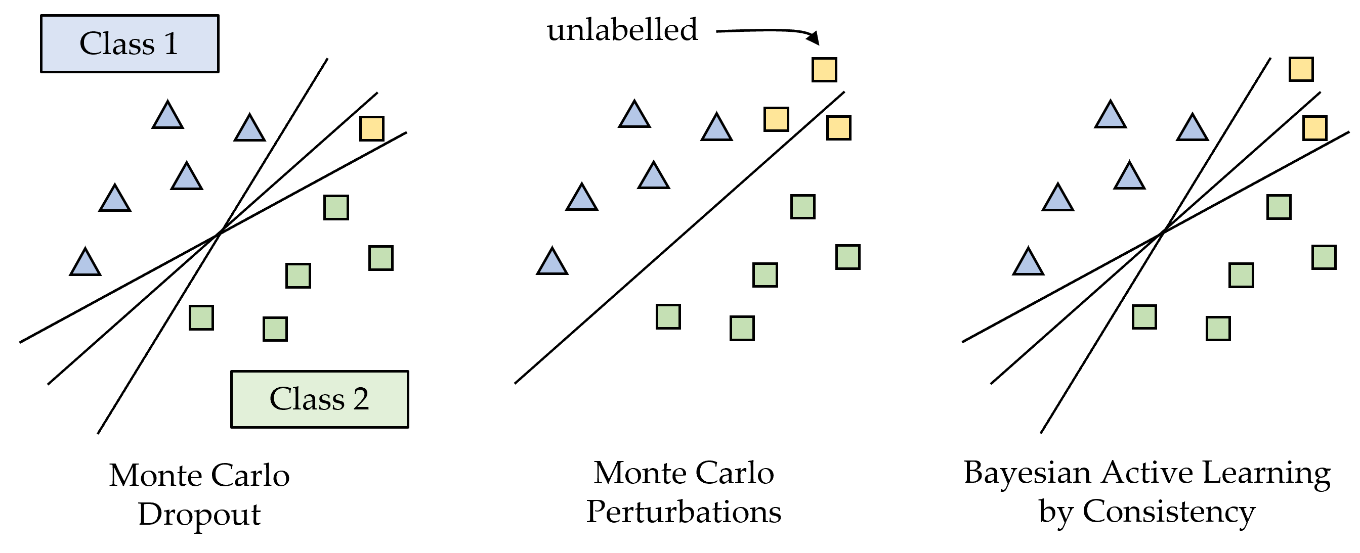
Figure 1: Perturbation frameworks used in active learning. Labelled instances from two classes and unlabelled instances (yellow) with the hypotheses of (Left) Monte Carlo Dropout (MCD), where each MC sample is a distinct hypothesis, (Centre) Monte Carlo Perturbations (MCP), with one hypothesis but several perturbed variants of the unlabelled instance, and (Right) Bayesian Active Learning by Consistency (BALC) with multiple hypotheses and perturbed instances. In this paper, we introduce MCP and BALC as alternatives to MCD in order to acquire unlabelled instances.

2 Related Work

2.1 Active Learning in Healthcare

For medical images, previous work has acquired instances by measuring their distance in a latent space to images in the training set (Smailagic et al., 2018, 2020). For time-series data, researchers have acquired instances from electronic health record (EHR) (Gong et al., 2019) and electrocardiogram (ECG) (Wiens & Guttag, 2010; Pasolli & Melgani, 2010; Wang et al., 2019; Kiyasseh et al., 2021a) databases. For example, although Kiyasseh et al. (2021a) acquire cardiac signals, they do so in the context of continual learning and do not explore how to annotate such cardiac signals. More generally, Gal et al. (2017) adopt BALD (Houlsby et al., 2011) in the context of Monte Carlo Dropout to acquire instances that maximize the Jensen-Shannon divergence (JSD) across MC samples. For an in-depth review of active learning, we refer readers to Settles (2009).

2.2 Oracles in Active Learning

Previous work attempts to learn from multiple or imperfect oracles (Dekel et al., 2012; Zhang & Chaudhuri, 2015; Sinha et al., 2019). For example, Urner et al. (Urner et al., 2012) identify a suitable oracle to label a particular instance. In contrast to our work, they do not explore the independence of a learner from an oracle. Although Yan et al. (2016) consider oracle abstention, we place the decision of abstention under the control of the learner. To the best of our knowledge, we are the first to explore a dynamic oracle selection strategy in the context of cardiac signals.

2.3 Consistency Training

Consistency training helps enforce the smoothness assumption (McCallumzy & Nigamy, 1998; Zhu, 2005; Verma et al., 2019). For example, Xie et al. (2019) penalize networks for generating drastically different outputs in response to perturbed instances, resulting in perturbation-invariant representations. Most similar to our work is that of Gao et al. (2020) which designs a consistency-loss based on the Kullback-Leibler divergence $\mathcal{D}_{KL}$. Whereas they actively acquire instances using the variance of the probability assigned to each class by the network in response to perturbed versions of the same instance, we design distinct consistency-based acquisition functions.

2.4 Selective Classification

Selective classification imbues a network with the ability to abstain from making predictions (Chow, 1970; El-Yaniv & Wiener, 2010; Cortes et al., 2016). Wiener & El-Yaniv (2011) use a support vector machine to rank and reject instances based on the degree of disagreement between hypotheses. In some frameworks, these are the same instances that active learning views as most informative. Although Liu et al. (2019) propose the gambler’s loss to learn a selection function that determines whether instances are rejected, this approach is not implemented in the context of active learning. SelectiveNet (Geifman & El-Yaniv, 2019) introduces a multi-head architecture similar to ours, however it assumes the presence of ground-truth labels and, therefore, does not trivially extend to unlabelled instances.

3 Background

3.1 Active Learning

Consider a learner $f_{\theta}:\boldsymbol{x}\in\mathbb{R}^{D}\rightarrow\boldsymbol{v}\in\mathbb{R}^{E}$, parameterized by $\boldsymbol{\theta}$, that maps a $D$-dimensional instance, $\boldsymbol{x}$, to an $E$-dimensional representation, $\boldsymbol{v}$. Further consider a function, $p_{\omega}:\boldsymbol{v}\in\mathbb{R}^{E}\rightarrow y\in\mathbb{R}^{C}$, that maps an $E$-dimensional representation, $\boldsymbol{v}$, to a $C$-dimensional output, $y$, where $C$ is the number of classes. After training on a pool of labelled data, $\mathcal{D}_{L}=\{\boldsymbol{X_{L}},\boldsymbol{Y_{L}}\}$ for $\tau$ epochs, the learner is tasked with querying the unlabelled pool of data, $\boldsymbol{X_{U}}$, and acquiring the top $b$ fraction of instances, $\{\boldsymbol{x}_{i}\}_{i=1}^{b}\sim\boldsymbol{X_{U}}$, that it deems to be most informative. The degree of informativeness of an instance, $\boldsymbol{x}$, is determined by an acquisition function, $\alpha(\boldsymbol{x})\in\mathbb{R}$, such as Bayesian Active Learning by Disagreement ($\mathrm{BALD}$) (Houlsby et al., 2011). These functions are typically used alongside Monte Carlo Dropout ($\mathrm{MCD}$) (Gal & Ghahramani, 2016) to identify instances that lie in the region of uncertainty, a region in which hypotheses disagree the most about instances (Fig. 1 left).

3.2 Consistency Training

Consider an unlabelled instance, $\boldsymbol{x}\sim\boldsymbol{X_{U}}$, and its perturbed counterpart, $\boldsymbol{x^{\prime}}=\boldsymbol{x}+\epsilon$, where $\epsilon$ is some perturbation. A network is said to be invariant to such a perturbation if its outputs, $p_{\omega}(\boldsymbol{x})$ and $p_{\omega}(\boldsymbol{x^{\prime}})$, are similar to one another. Consistency training is one way to encourage such an invariance. In this work, we exploit this intuition to design acquisition functions, as outlined next.

4 Methods

4.1 Monte Carlo Perturbations

Acquisition functions dependent upon parameter perturbations, such as in $\mathrm{MCD}$, can overlook, and thus fail to acquire, informative unlabelled instances. To see this, and without loss of generality, consider an unlabelled instance which is (a) in proximity to a decision boundary, thus deeming it informative for training (Settles, 2009) and (b) classified by a network into an arbitrary class. In this setting, a total of $T$ parameter perturbations results in $T$ hypotheses, altering the outputs of a network, $\{p_{\omega}^{i}\}_{i=1}^{T}$, in response to an unlabelled instance. We visualize the distribution of such outputs in Fig. 2 (red rectangle), after having applied $T=3$ parameter perturbations. If the perturbations happen to be too small in magnitude, for example, then a network will exhibit a similar output distribution ($p_{\omega}^{1}=p_{\omega}^{2}=\cdots$) across the parameter perturbations. However, since acquisition functions assign value based on changes in the output distribution, this informative unlabelled instance (due to its proximity to decision boundary) would be erroneously deemed uninformative.

One way to avoid missing these informative instances is by stochastically perturbing instances (instead of network parameters) and observing changes in the network outputs, a setup we refer to as Monte Carlo Perturbations ($\mathrm{MCP}$). This results in a single hypothesis but multiple perturbed variants of the instance (see Fig. 1 centre). The intuition is that network outputs will differ more significantly for an instance in proximity to the decision boundary than for an instance farther away. By quantifying these output changes, as is done with almost any acquisition function, we can identify informative instances for acquisition. The main advantage of MCP over MCD is the increased control and interpretability of the applied perturbations; perturbations applied to instances are likely to be more understandable than those applied to parameters. A formal derivation of $\mathrm{MCP}$ can be found Appendix A.

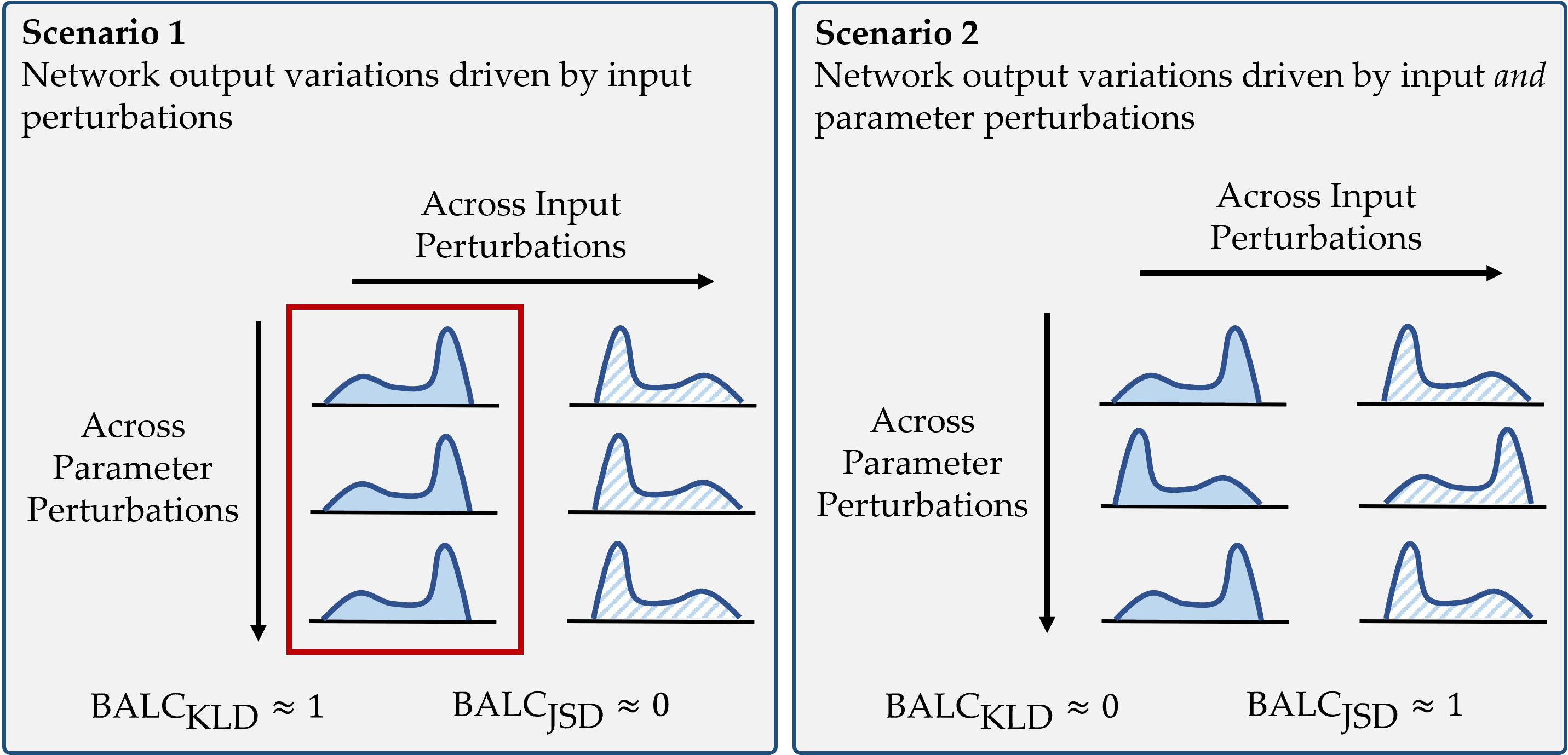
Figure 2: Scenarios demonstrating the effect of input and parameter perturbations on the behaviour of the proposed acquisition functions, $\mathrm{BALC}_{\mathrm{KLD}}$ and $\mathrm{BALC}_{\mathrm{JSD}}$. (Scenario 1) network output variations caused primarily by input perturbations. The red rectangle illustrates how parameter perturbations alone, as with MCD, can be insufficient in causing changes to the network outputs, thus failing to acquire informative unlabelled instances. (Scenario 2) network output variations caused by both input and parameter perturbations. We show that while $\mathrm{BALC}_{\mathrm{KLD}}$ is likely to acquire instances due to input perturbations, $\mathrm{BALC}_{\mathrm{JSD}}$ considers both input and parameter perturbations when performing acquisitions.

4.2 Bayesian Active Learning by Consistency

It could be argued that the same limitations exhibited by MCD also extend to MCP. After all, both frameworks apply perturbations to either network parameters or instances. Acknowledging this, we propose a framework, entitled Bayesian Active Learning by Consistency ($\mathrm{BALC}$), in which perturbations are simultaneously applied to network parameters and instances. As such, this results in multiple decision boundaries and perturbed instances (see Fig. 1 right). $\mathrm{BALC}$ consists of three main steps: 1) perturb an instance, $\boldsymbol{x}\in\mathbb{R}^{D}$, to generate $\boldsymbol{x^{\prime}}\in\mathbb{R}^{D}$, 2) perturb the network parameters, $\boldsymbol{\theta}$, to generate $\boldsymbol{\theta^{\prime}}$, and 3) pass both instances, $\boldsymbol{x}$ and $\boldsymbol{x^{\prime}}$, through the perturbed network, generating outputs, $p(y|\boldsymbol{x},\boldsymbol{\theta^{\prime}})$ and $p(y|\boldsymbol{x^{\prime}},\boldsymbol{\theta^{\prime}})\in\mathbb{R}^{C}$, respectively. Note that we drop the explicit dependence on $\boldsymbol{\omega}$ for clarity. We perform these steps for $T$ stochastic parameter perturbations and generate two matrices of network outputs, $\boldsymbol{G(x)},\boldsymbol{G^{\prime}(x^{\prime})}\in\mathbb{R}^{T\times C}$, as shown in Fig. 3.

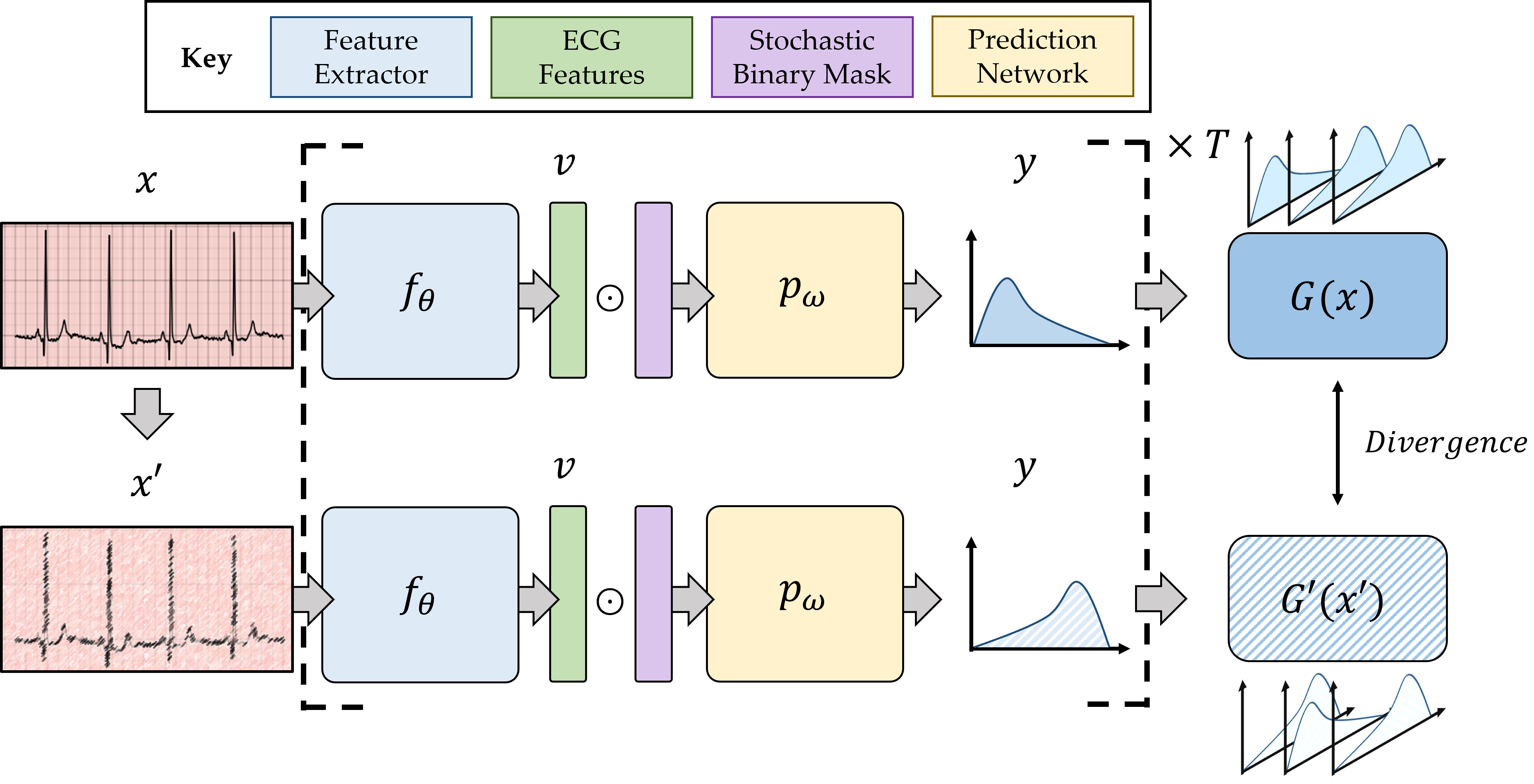
Figure 3: Consistency-based active-learning framework. We perturb an instance, $\boldsymbol{x}$, to generate, $\boldsymbol{x^{\prime}}$, and extract their corresponding representations, $v$. We apply a stochastic dropout mask to these representations and obtain an output distribution over the classes. When repeated $T$ times, this generates a pair of matrices, $\boldsymbol{G(x)}$ and $\boldsymbol{G^{\prime}(x^{\prime})}$, whose divergence is calculated via $\mathrm{BALC}_{\mathrm{KLD}}$ or $\mathrm{BALC}_{\mathrm{JSD}}$.

The intuition is that the greater the divergence between $\boldsymbol{G}$ and $\boldsymbol{G^{\prime}}$, the closer an instance is to the decision boundary. To that end, we propose two consistency-based acquisition functions, $\mathrm{BALC}_{\mathrm{KLD}}$ and $\mathrm{BALC}_{\mathrm{JSD}}$.

To calculate $\mathrm{BALC}_{\mathrm{KLD}}(\boldsymbol{x})\in\mathbb{R}$ (1), we first empirically fit two $C$-dimensional Gaussian distributions, $\mathcal{N}(\boldsymbol{x})$ and $\mathcal{N}(\boldsymbol{x^{\prime}})$ to $\boldsymbol{G}$ and $\boldsymbol{G^{\prime}}$, respectively. For each such matrix, we obtain an empirical mean vector, $\boldsymbol{\mu}=\frac{1}{T}\sum_{i}^{T}\boldsymbol{G}_{i}$ and covariance matrix, $\boldsymbol{\Sigma}=(\boldsymbol{G}-\boldsymbol{\mu})^{T}(\boldsymbol{G}-\boldsymbol{\mu})$. We then quantify the $D_{KL}$ between $\mathcal{N}(\boldsymbol{x})$ and $\mathcal{N}(\boldsymbol{x^{\prime}})$ as follows.

$$\mathrm{BALC}_{\mathrm{KLD}}(\boldsymbol{x})=\mathcal{D}_{KL}(\mathcal{N}(\boldsymbol{x})\;\|\;\mathcal{N}(\boldsymbol{x^{\prime}}))$$ (1)

where $\mathcal{N}(\boldsymbol{x})=\mathcal{N}(\boldsymbol{\mu(x)},\boldsymbol{\Sigma(x)})$ and $\mathcal{N}(\boldsymbol{x^{\prime}})=\mathcal{N}(\boldsymbol{\mu(x^{\prime})},\boldsymbol{\Sigma(x^{\prime})})$.

We note that $\mathrm{BALC}_{\mathrm{KLD}}$ is likely to detect changes in the network outputs due solely to instance perturbations. To see this, consider Scenario 1 and 2 presented in Fig. 2. Changes in network outputs are caused by either instance perturbations alone (Scenario 1) or both instance and parameter perturbations (Scenario 2). In these two scenarios, $\mathrm{BALC}_{\mathrm{KLD}}\approx 1$ and $0$, respectively. Since the informativeness of an instance is related to the magnitude of the acquisition function, these scenarios suggest that $\mathrm{BALC}_{\mathrm{KLD}}$ has a preference for instance perturbations. In order to detect changes in the network outputs due to both instance and parameter perturbations, we introduce $\mathrm{BALC}_{\mathrm{JSD}}$. Support for this claim can also be found in Fig. 2.

$\mathrm{BALC}_{\mathrm{JSD}}(\boldsymbol{x})\in\mathbb{R}$ (2) comprises the difference of two terms. The first term, , calculates the $D_{KL}$ of network outputs due to a single instance perturbation and averages this across $T$ parameter perturbations. The second term, , averages the network outputs across parameter perturbations independently for the original and perturbed instance before calculating the $D_{KL}$ of the resulting mean outputs. The full derivation of $\mathrm{BALC}_{\mathrm{JSD}}$ can be found in Appendix A.

$$\begin{split}\text{BALC}_{\text{JSD}}(\boldsymbol{x})&=\overbrace{\frac{1}{T}\sum_{i=1}^{T}\left[\mathcal{D}_{KL}(\boldsymbol{G_{i}(x)}\;\|\;\boldsymbol{G^{\prime}_{i}(x^{\prime})})\right]}^{\text{ \leavevmode\hbox to10.32pt{\vbox to10.32pt{\text{[drawing]}}} across parameter perturbations}}-\\ &\overbrace{\mathcal{D}_{KL}(\frac{1}{T}\sum_{i=1}^{T}\boldsymbol{G_{i}(x)}\;\|\;\frac{1}{T}\sum_{i=1}^{T}\boldsymbol{G^{\prime}_{i}(x^{\prime})})}^{\text{ \leavevmode\hbox to10.08pt{\vbox to10.08pt{\text{[drawing]}}} across input perturbations}}\end{split}$$ (2)

4.3 Tracked Acquisition Function

So far, we have discussed active learning frameworks that, similar to those in the literature, quantify the informativeness of an unlabelled instance at a single snapshot in time (e.g., at a particular epoch, $\tau$). This static setup, however, faces two limitations. First, it depends on an appropriate choice of epoch for the acquisition of instances, which is non-trivial to identify a priori. For example, an acquisition function can be of little value if calculated when network parameters have yet to be updated sufficiently. Second, the diversity and number of hypotheses obtained via parameter perturbations can be limited by this single-epoch view. This is detrimental given the established benefit of eliminating unsuitable hypotheses at a greater rate ($\downarrow$ version space) (Cohn et al., 1994).

To overcome such limitations, we propose to track this acquisition function over time (e.g., epochs) before deploying it for the acquisition of instances. This is a simple extension to almost any acquisition function. In the process, we become less dependent on the choice of acquisition epoch and are likely to increase the diversity of hypotheses at our disposal. Formally, consider an acquisition function, $\alpha(\boldsymbol{x})$, which would ordinarily be calculated once at epoch, $\tau$, for each instance, $\boldsymbol{x}$. In our formulation, we calculate $\alpha(\boldsymbol{x},t)$ at each epoch, $t\in[1,\tau]$. At epoch, $\tau$, which we refer to as an acquisition epoch, the modified acquisition function, $\mathrm{AUTAF(\boldsymbol{x},\alpha)}\in\mathbb{R}$, corresponds to the area under the tracked acquisition function, approximated via the trapezoidal rule.

$$\begin{split}\text{AUTAF}(\boldsymbol{x},\alpha)&\approx\sum_{t=1}^{\tau}\left(\frac{\alpha(\boldsymbol{x},t+\Delta t)+\alpha(\boldsymbol{x},t)}{2}\right)\Delta t\end{split}$$ (3)

where $\Delta t$ is the interval between epochs at which acquisition values are calculated.

4.4 Selective Oracle Questioning

Up until this point, we have discussed methods that exclusively target the acquisition of unlabelled instances. We now direct our attention to the annotation of such instances with the goal of minimizing the labelling burden that is placed on an oracle. To do so, we design a framework that, given an acquired unlabelled instance, dynamically determines whether to request a label from an oracle or to pseudo-label that instance instead. This framework, which we refer to as selective oracle questioning in active learning, SoQal, is outlined next.

Oracle selection network

Let us first consider a learner, $g_{\phi}:\boldsymbol{v}\in\mathbb{R}^{E}\rightarrow r\in[0,1]$, parameterized by $\boldsymbol{\phi}$, that maps an $E$-dimensional representation, $\boldsymbol{v}$, to a scalar, $r$, as shown in Fig. 4. We refer to this learner as an oracle selection network.

Learning a proxy for misclassifications

The intuition underlying our oracle selection framework is as follows. Given an instance, a network should request a label (i.e., ask for help) from an oracle instead of pseudo-label it if the network is likely to misclassify this instance. This idea operates under the assumption that the network is able to identify whether an instance will be misclassified. While this is possible with labelled data, it is non-trivial with unlabelled data (due to absence of a ground-truth), the prime focus of active learning. As such, we need a way to identify whether an unlabelled instance would have been misclassified if it were to be pseudo-labelled by the network. In other words, we need a reliable proxy for a misclassification.

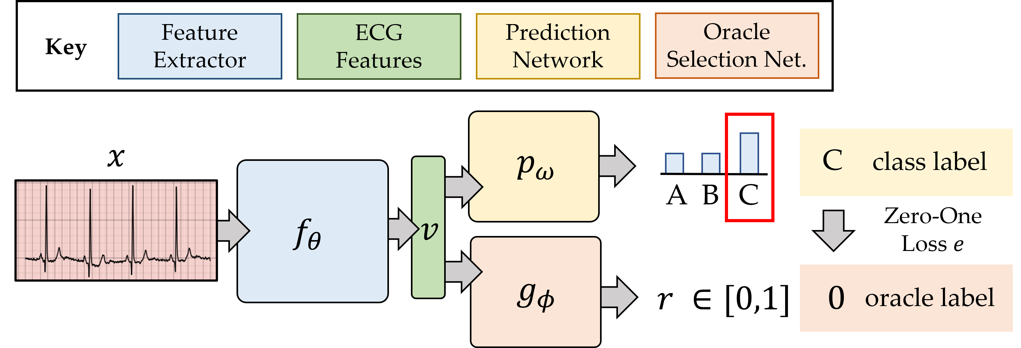
Figure 4: Selective oracle questioning framework. Representation, $\boldsymbol{v}$, of instance, $\boldsymbol{x}$ is passed through $p_{\omega}$ to generate task predictions and $g_{\phi}$ to determine whether a label is requested from an oracle. The zero-one loss of $p_{\omega}$ is the ground-truth label for $r$. High (low) values of $r$ indicate that an instance should be labelled by an oracle (pseudo-labelled by prediction network).

To design this proxy, we exploit the oracle selection network ($g_{\phi}$) and its scalar output, $r$. As we explain next, we learn $\boldsymbol{\phi}$ such that higher values of $r$ correspond to misclassifications. Achieving this requires that $r$ have a supervisory ground-truth label. We choose such a label to be the zero-one loss, $e\in\mathbb{R}$, incurred by the prediction network, $p_{\omega}$, on an instance, $\boldsymbol{x}$. Intuitively, when $e=1$, the network should request a label from an oracle. Note that this ground-truth label, $e$, is only available while training on labelled data. We later explain how to exploit $r$ on acquired unlabelled instances. As such, while training on labelled data, we optimize (4) with a categorical cross-entropy loss for the prediction network, $\mathcal{L}_{CPL}$, with ground-truth class labels, $c$, and a weighted binary cross-entropy loss for the oracle selection network, $\mathcal{L}_{OSL}$. In the process, we learn the parameters, $\boldsymbol{\theta}$, $\boldsymbol{\omega}$, and $\boldsymbol{\phi}$ in an end-to-end manner.

$$\begin{split}\mathcal{L}=\mathcal{L}_{CPL}+\mathcal{L}_{OSL}\end{split}$$ (4)

$$\mathcal{L}_{CPL}=-\sum_{i=1}^{B}\log\left(p_{\boldsymbol{\omega}}(y_{i}=c|\boldsymbol{x}_{i},\boldsymbol{\phi})\right)$$

$$\mathcal{L}_{OSL}=-\sum_{i=1}^{B}\beta e_{i}\log g_{\boldsymbol{\phi}}(\boldsymbol{x}_{i})-(1-e_{i})\log\left(1-g_{\boldsymbol{\phi}}(\boldsymbol{x}_{i})\right)$$

Weighted oracle selection loss. During the early stages of training on labelled data, a network struggles to classify instances correctly. In our framework, this implies that we will encounter more terms with $e=1$ (misclassification) than those with $e=0$ (correct classification). The opposite is true as training progresses and the network becomes more adept at classifying instances. Therefore, regardless of the stage of training (early vs. late), there will be an imbalance in the ground-truth labels, $e$, provided to the oracle selection network. This imbalance sends a strong supervisory signal to $g_{\phi}$ through the oracle selection loss, $\mathcal{L}_{OSL}$, and not accounting for it would lead to systematically higher (lower) $r$ values during the early (late) stages of training. This can reduce the reliability of $r$ as a proxy for misclassifications. As such, we introduce a dynamic weight, $\beta=\frac{\sum\mathbbm{1}({e=0})}{\sum\mathbbm{1}({e=1})}$, where $\mathbbm{1}$ is the indicator function. As training progress, $\beta<1\rightarrow\beta>1$, as the ratio of correctly classified ($e=0$) to misclassified ($e=1$) instances within a mini-batch changes.

Making decisions with proxy

We exploit $r$ for the binary decision of whether to request a label from an oracle or to generate a pseudo-label instead. Since $r\in[0,1]$, one simple rule would be to select an oracle if $r>0.5$. This threshold, however, may be sub-optimal particularly if the values of $r$ are not calibrated. Therefore, to design a robust rule, we account for the distribution of the $r$ values stratified according to the zero-one loss, $e$, on labelled data, and the separability of such distributions. We present such empirical stratified distributions in Figs. 5(a) and 5(b) during the early and late stages of training, respectively. As expected, we find that correctly-classified instances ($e=0$) tend to have lower $r$ values than those which are misclassified.

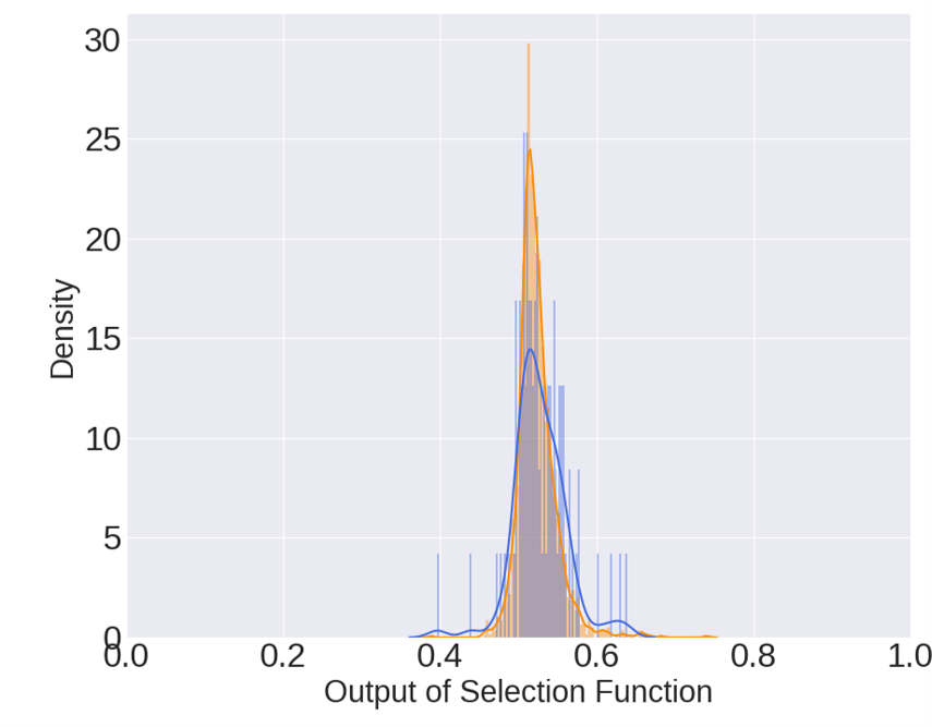
(a) Early stage

(b) Late stage

(c) $D_{H}$

Figure 5: Components of selective oracle questioning framework. Distribution of the outputs, $r$, of $g_{\phi}$ stratified based on the zero-one loss, $e$ during the (a) early and (b) late stages of training. (c) Hellinger distance, $D_{H}$, between the two distributions of $r$ increases during training.

We now outline the steps involved in making the binary decision. First, after each training epoch, $t$, we fit two unimodal Gaussian distributions, $\mathcal{N}_{0}(\mu_{0},\sigma_{0}^{2})$ and $\mathcal{N}_{1}(\mu_{1},\sigma_{1}^{2})$ corresponding to $e=0$ and $e=1$, respectively, to the $r$ values (generated on the labelled data), similar to those in Fig. 5(b). Low separability of such distributions would suggest that the oracle selection network has yet to learn to distinguish between correctly-classified and misclassified instances, and is thus generating an unreliable proxy, $r$. We quantify this separability via the Hellinger distance, $D_{H}\in[0,1]$, a metric to which a threshold can be easily applied. In Fig. 5(c), we show that indeed as training progresses, the separability of the two distributions increases, which is suggestive of an increasingly reliable proxy. Based on some user-defined threshold, $S$, low separability (i.e., low proxy reliability) can be defined as $D_{H}<S$. In such an event, we use a conservative strategy that defers labelling to the oracle. This value of $S$ can be altered depending on the relative level of trust placed in the network and oracle.

Pseudo-labelling. High separability, defined as $D_{H}\geq S$ suggests that the proxy is sufficiently reliable to make decisions. As such, for each acquired unlabelled instance, $\boldsymbol{x}_{u}\sim\boldsymbol{X_{U}}$, we obtain $r_{u}=g_{\boldsymbol{\phi}}(\boldsymbol{x}_{u})$ and compare the values of $\mathcal{N}_{0}$ and $\mathcal{N}_{1}$ when evaluated at $r_{u}$. If $\mathcal{N}_{1}>\mathcal{N}_{0}$, then the value of $r$ is too high (indicating a potential network misclassification), and a label is requested from an oracle. Otherwise, the instance is pseudo-labelled via $\operatorname*{argmax}_{c}p_{\omega}(y=c|\boldsymbol{x})$. The probability of requesting a label from an oracle is denoted by $p(\text{A})$.

$$p(\text{A})=\begin{dcases}1,&D_{H}<S\\ 1,&\mathcal{N}_{1}>\mathcal{N}_{0}\ \text{and}\ D_{H}\geq S\\ 0,&\text{otherwise}\\ \end{dcases}$$ (5)

where $\mathcal{N}_{1}=\mathcal{N}\left(r=r_{u}|\mu_{1},\sigma_{1}^{2},e=1\right)$ and $\mathcal{N}_{0}=\mathcal{N}\left(r=r_{u}|\mu_{0},\sigma_{0}^{2},e=0\right)$. We note that our oracle selection framework is independent of the acquisition of unlabelled instances, making it general enough to be used alongside almost any acquisition function. Pseudo-code for the entire pipeline can be found in Appendix A.

5 Experimental Design

5.1 Datasets

We conduct our experiments using PyTorch (Paszke et al., 2019) on four publicly-available datasets comprising cardiac signals, such as the photoplethysmogram (PPG) and the electrocardiogram (ECG) alongside cardiac arrhythmia labels (abnormalities in the functioning of the heart). PhysioNet 2015 ($\mathcal{D}_{1}$) (Clifford et al., 2015) consists of PPG data alongside 5 different classes of cardiac arrhythmia. $\mathcal{D}_{2}$ is similar to the first however comprises ECG data. PhysioNet 2017 ($\mathcal{D}_{3}$) (Clifford et al., 2017) consists of 8,528 single-lead ECG recordings alongside 4 different classes of cardiac arrhythmia. Cardiology ($\mathcal{D}_{4}$) (Hannun et al., 2019) consists of single-lead ECG data from 292 patients alongside 12 different classes of cardiac arrhythmia.

In order to evaluate our framework in the limited data regime, we place a fraction, $F\in[0.1,0.3,0.5,0.7,0.9]$, of the training dataset into a labelled set, $\mathcal{D}_{L}$. and its complement into an unlabelled set, $\boldsymbol{X_{U}}$ (see Table 1). Additional details about the datasets and pre-processing steps can be found in Appendix A.

	Train		Val.	Test
Dataset	Labelled	Unlabelled
$\mathcal{D}_{1}$	401	4233	1124	1435
$\mathcal{D}_{2}$	401	4233	1124	1435
$\mathcal{D}_{3}$	1,776	16,479	4,582	5,824
$\mathcal{D}_{4}$	452	4,110	1,131	1,386

Table 1: Number of instances in the training, validation, and test sets. The distribution of labelled instances is shown for a fraction, $F=0.1$, of the original training set. This is also used for the selective oracle questioning experiments. The remaining distributions can be found in Appendix A.

5.2 Network Architecture

Our network architecture involves a lightweight convolutional network which receives a cardiac time-series segment (2500 samples or $\approx$ 5 seconds in duration) as input and returns a probability distribution over cardiac arrhythmias as output. We chose this architecture based on previous research demonstrating its effectiveness in classifying cardiac arrhythmias (Kiyasseh et al., 2021b). Additional details about the network architecture can be found in Appendix A.

5.3 Active Learning Scenarios

We explore three distinct active learning scenarios characterized by the presence and quality of an oracle. Recall that the motivation behind our framework was to exploit abundant unlabelled and limited labelled data while alleviating (and not necessarily eliminating) the labelling burden placed on an oracle. As such, the target and realistic clinical scenario in which our framework would be deployed is one where an oracle (e.g., physician) is available in some capacity. However, to explore the extreme limits of our approach, and as a stepping stone to the target clinical scenario, we begin our experimentation without an oracle and transition to the scenarios in which an oracle is available.

Scenario 1 - Without Oracle. we assume that a physician is unavailable to provide labels and thus evaluate the performance of our framework without an oracle.

Scenario 2 - Noise-free Oracle. we assume that a physician is available and capable of providing accurate labels.

Scenario 3 - Noisy Oracle. we assume that a physician is either ill-trained or unable to perform a diagnosis due to its difficulty. To simulate this setting, we introduce two types of label noise. We stochastically flip the ground-truth label (unseen by the network) of each unlabelled instance to 1) (Random) any other label randomly, or 2) (Nearest Neighbour) its nearest neighbour, in a smaller dimensional subspace, from a different class. Whereas the first form of noise is extreme, the latter is more realistic as it may reflect uncertain physician diagnoses. Furthermore, we simulate noise of different magnitude by injecting it with probability $\gamma=[0.05,0.1,0.2,0.4,0.8]$.

5.4 Baselines

We compare our proposed acquisition functions to the state-of-the-art functions used alongside MCD. These include Var Ratio, Entropy, and BALD (Houlsby et al., 2011), definitions of which can be found in Appendix A. We also experiment with several baselines that exhibit varying degrees of oracle dependence. $\epsilon$-greedy (Watkins, 1989) - a stochastic strategy that we adapt to exponentially decay the reliance of the network on an oracle as a function of the number of acquisition epochs. $S$-response - assumes that high entropy predictions are indicative of instances that the network is unsure of. Therefore, we introduce a threshold, $S_{\mathrm{Entropy}}$, such that if it is exceeded, an oracle is requested to label the chosen instance (see Appendix A).

5.5 Hyperparameters

For all experiments, we chose the number of MC samples $T=20$ to balance between computational complexity and accuracy of the approximation of the version space. During training, we acquire unlabelled instances at pre-defined epochs (acquisition epochs), $\tau=5n$, $n\in\mathbb{N}^{+}$. During each acquisition epoch, we acquire $b=2\%$ of the remaining unlabelled instances. We investigate the effect of such hyperparameters on performance in Appendices LABEL:appendix:effect_of_mcsamples-LABEL:appendix:effect_of_aqinterval. When experimenting with tracked acquisition functions, we chose the temporal period, $\Delta t=1$, calculating the acquisition function at each epoch of training. Given the increasing trend of $D_{H}$ during training (see Fig. 5(c)), we chose $D_{H}\geq S=0.15$ to balance between the reliability of the proxy and the independence of the network from an oracle.

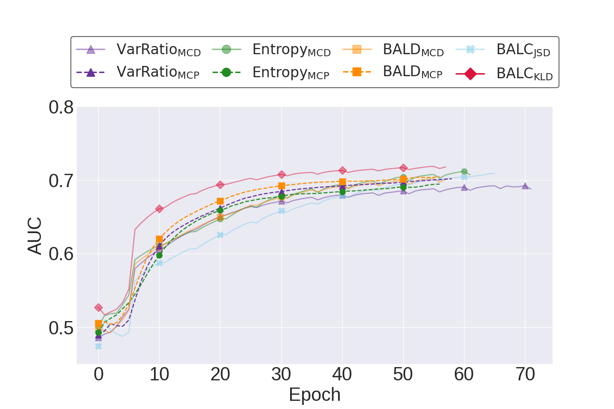
(a) $\mathcal{D}_{2}$ at $F=0.3$

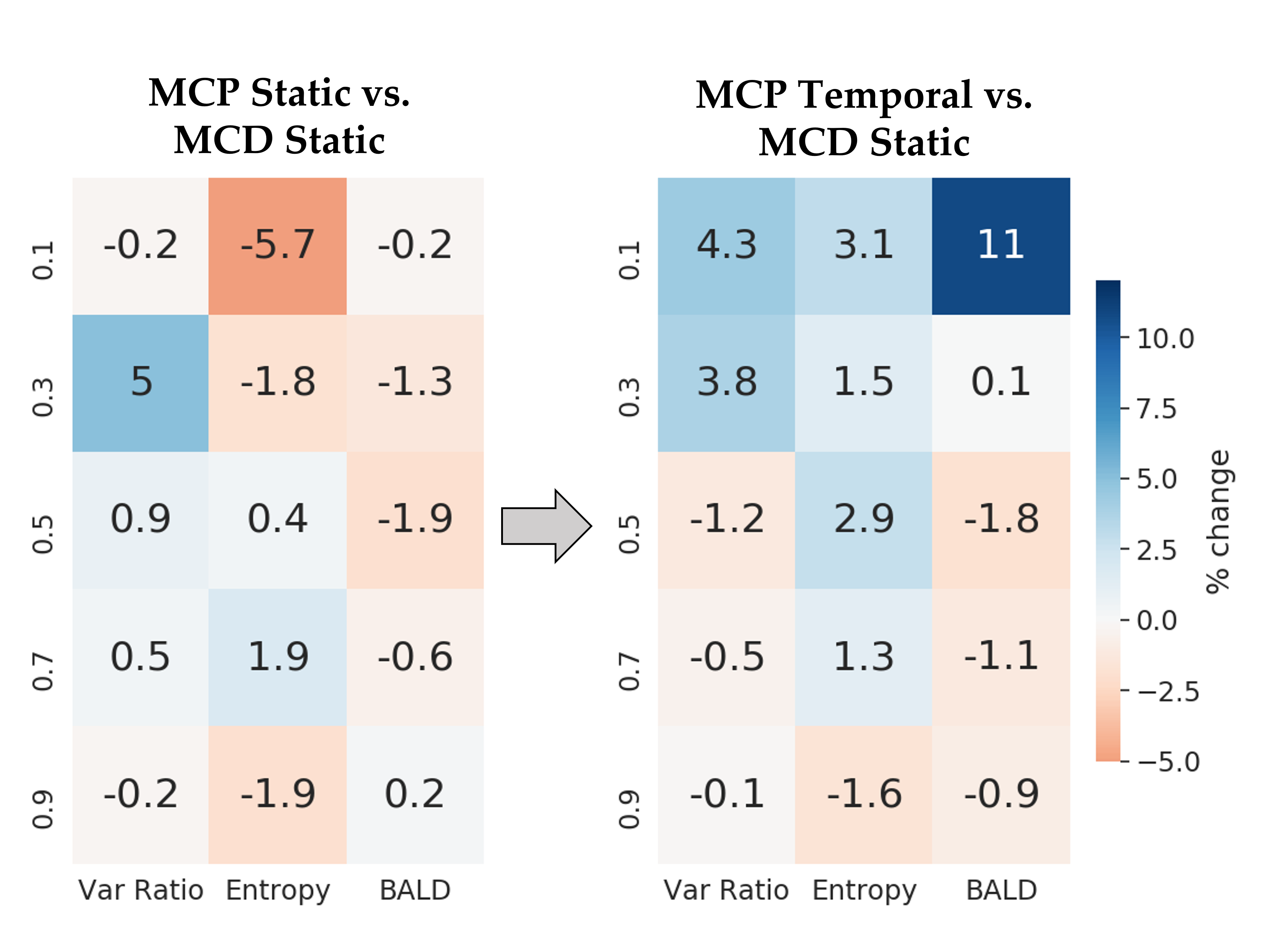
(b) Utility of tracked acquisition functions on $\mathcal{D}_{1}$

Figure 6: Performance of active learning frameworks without an oracle. (a) Validation AUC on $\mathcal{D}_{2}$ at $F=0.3$. (b) Percent change in AUC when comparing MCP with static and temporal acquisition functions to MCD with static functions on $\mathcal{D}_{1}$. Results are averaged across five seeds. In (a), we show that $\mathrm{BALC}_{\mathrm{KLD}}$ can outperform state-of-the-art acquisition functions. In (b), we show the marginal benefit of temporal acquisition functions.

6 Experimental Results

6.1 Active Learning without Oracle

We begin by exploring the performance of active learning frameworks without an oracle. In Fig. 6(a), we illustrate the validation AUC of a network that is initially exposed to $F=0.3$ of the labelled training data of $\mathcal{D}_{2}$.

We find that a network which exploits $\mathrm{BALC}_{\mathrm{KLD}}$ learns faster than, and outperforms, those which exploit the remaining acquisition functions. For example, $\mathrm{BALC}_{\mathrm{KLD}}$ and $\mathrm{BALD}_{\mathrm{MCD}}$ achieve $\mathrm{AUC}\approx 0.69$ after $20$ and $40$ epochs of training, respectively, reflecting a two-fold increase in learning efficiency. Moreover, $\mathrm{BALC}_{\mathrm{KLD}}$ and $\mathrm{Entropy}_{\mathrm{MCD}}$ achieve a final $\mathrm{AUC}\approx 0.72$ and $\approx 0.70$, respectively. One hypothesis for this improved performance is that $\mathrm{BALC}_{\mathrm{KLD}}$, as a consistency-based active learning framework, acquires unlabelled instances which may still be correctly pseudo-labelled by the network despite the absence of an oracle. This, in turn, facilitates learning. Uncertainty-based acquisition functions, on the other hand, acquire unlabelled instances to which the network is most uncertain. As such, pseudo-labels for these instances are likely to be incorrect. The results for the remaining experiments can be found in Appendix LABEL:appendix:effect_of_perturbations.

We now transition to quantifying the marginal benefit of incorporating temporal information into the acquisition functions. In Fig. 6(b), the panel on the left illustrates the percent change in the AUC when comparing $\mathrm{MCP}$ to $\mathrm{MCD}$ while using static acquisition functions. The panel on the right, however, depicts the results after having incorporated temporal information into the acquisition functions used alongside $\mathrm{MCP}$. Hence, the naming $\mathrm{MCP\ Temporal}$. We find that tracked acquisition functions add value when the size of the labelled dataset is small ($\downarrow F$) (red rectangle). For example, transitioning from $\mathrm{MCP\ Static}$ to $\mathrm{MCP\ Temporal}$ when exploiting $\mathrm{BALD}$ at $F=0.1$ improves the $\mathrm{AUC}$ by $11\%$. Similar improvements can be seen in Appendix LABEL:appendix:effect_of_temporal_functions. We hypothesize that this improvement is due to the increased diversity, and number, of hypotheses available when considering temporal information, thus eliminating unsuitable hypotheses at a greater rate.

Dataset	Ac. Function $\alpha$	Oracle Questioning Method
		$S$-response	$\epsilon$-greedy	SoQal
$\mathcal{D}_{1}$	$\mathrm{BALD_{MCD}}$	49.6 (3.9)	49.1 (2.8)	62.1 (2.1)
	$\mathrm{BALD_{MCP}}$	51.7 (4.3)	50.1 (4.3)	64.5 (1.5)
	$\mathrm{BALC_{KLD}}$	54.8 (3.4)	54.8 (4.2)	59.8 (5.5)
	Temp. $\mathrm{BALC_{KLD}}$	53.6 (4.0)	52.1 (5.9)	64.6 (6.7)
$\mathcal{D}_{2}$	$\mathrm{BALD_{MCD}}$	58.4 (4.1)	60.9 (7.1)	70.7 (3.8)
	$\mathrm{BALD_{MCP}}$	63.8 (4.3)	63.7 (4.4)	67.7 (4.2)
	$\mathrm{BALC_{KLD}}$	58.2 (1.7)	64.3 (3.3)	67.7 (2.4)
	Temp. $\mathrm{BALC_{KLD}}$	61.2 (5.0)	60.5 (1.9)	64.8 (5.7)
$\mathcal{D}_{3}$	$\mathrm{BALD_{MCD}}$	58.8 (1.3)	67.3 (1.5)	72.1 (2.5)
	$\mathrm{BALD_{MCP}}$	67.6 (5.8)	66.5 (2.8)	72.0 (4.4)
	$\mathrm{BALC_{KLD}}$	62.9 (0.4)	64.3 (4.1)	73.1 (3.3)
	Temp. $\mathrm{BALC_{KLD}}$	63.0 (1.4)	65.4 (1.9)	73.0 (2.4)
$\mathcal{D}_{4}$	$\mathrm{BALD_{MCD}}$	48.9 (3.0)	47.4 (3.7)	46.8 (2.1)
	$\mathrm{BALD_{MCP}}$	50.4 (2.6)	49.2 (2.4)	49.9 (2.9)
	$\mathrm{BALC_{KLD}}$	50.4 (3.9)	47.3 (1.0)	49.5 (1.2)
	Temp. $\mathrm{BALC_{KLD}}$	49.6 (2.3)	49.6 (2.3)	50.3 (1.0)

Table 2: Test AUC of oracle questioning methods with a noise-free oracle at $F=0.1$. Mean (standard deviation) is presented across five random seeds for $\mathcal{D}_{1}-\mathcal{D}_{4}$. Bold indicates top-performing method. We show that SoQal outperforms $S$-response and $\epsilon$-greedy across $\mathcal{D}_{1}-\mathcal{D}_{3}$.

6.2 Active Learning with Noise-free Oracle

Having explored the performance of active learning frameworks without an oracle, we now assume the presence of a noise-free oracle and explore the effect of selective oracle questioning methods. In Table 2, we present the results of these experiments across all datasets at $F=0.1$.

We find that $\mathrm{SoQal}$ consistently outperforms $S$-response and $\epsilon$-greedy across $\mathcal{D}_{1}$ - $\mathcal{D}_{3}$. For example, when using $\mathrm{BALD}_{\mathrm{MCD}}$ on $\mathcal{D}_{2}$, $\mathrm{SoQal}$ achieves $\mathrm{AUC}=70.7$ whereas $S$-response and $\epsilon$-greedy achieve $\mathrm{AUC}=58.4$ and $60.9$, respectively. Such a finding suggests that $\mathrm{SoQal}$ is well equipped to know when a label should be requested from an oracle. This improved performance also coincides with reduced dependence on an oracle (see Appendix LABEL:appendix:soqal_oracle_dependence). We also hypothesize that the poor performance of all methods on $\mathcal{D}_{4}$ is due to the cold-start problem (Konyushkova et al., 2017) where network learning is hindered by the limited availability of initial labelled training data. We support this claim with further experiments in Appendix LABEL:appendix:soqal_oracle_dependence.

6.3 Active Learning with Noisy Oracle

Building on the findings in the previous section, we now explore the performance of our oracle questioning methods with a noisy oracle. In Fig. 7, we illustrate the test $\mathrm{AUC}$ on $\mathcal{D}_{1}$ as a function of various types and levels of noise. We also present the performance with a noise-free oracle (horizontal dashed lines).

We find that $\mathrm{SoQal}$ is more robust to a noisy oracle than $\epsilon$-greedy and $S$-response. This is evident by the $\uparrow\mathrm{AUC}$ of the former relative to the latter across different noise types and magnitudes (except at $\gamma=0.4$ random noise). For example, at $5\%$ random noise, $\mathrm{SoQal}$ achieves $\mathrm{AUC}\approx 0.66$ whereas $\epsilon$-greedy and $S$-response achieve $\mathrm{AUC}\approx 0.56$ and $0.53$, respectively. We also find that $\mathrm{SoQal}$, in the presence of noise, continues to outperform the baseline methods in the absence of noise. For example, at $80\%$ nearest neighbour noise, $\mathrm{SoQal}$ achieves $\mathrm{AUC}\approx 0.59$ whereas $\epsilon$-greedy and $S$-response without label noise achieve $\mathrm{AUC}\approx 0.50$ and $0.52$, respectively. We arrive at similar conclusions for other datasets and acquisition functions (see Appendix LABEL:appendix:effect_of_label_noise). One hypothesis for this improved performance is that $\mathrm{SoQal}$, by appropriately deciding when to not request a label from a noisy oracle, avoids an incorrect instance annotation, and thus allows the network to learn well.

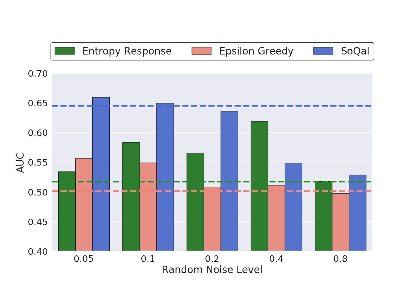
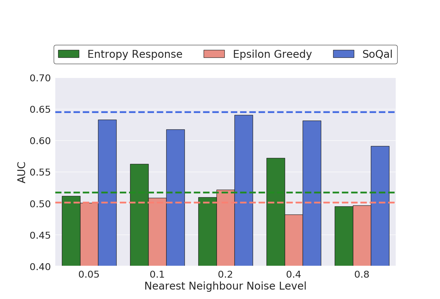
Figure 7: Test AUC of the oracle questioning methods with (left) random and (right) nearest neighbour label noise on $\mathcal{D}_{1}$ while using $\mathrm{BALD}_{\mathrm{MCP}}$. Horizontal dashed lines indicate performance of network without label noise. $\mathrm{SoQal}$, even with a noisy oracle, outperforms baseline methods with a noise-free oracle.

7 Discussion

In this paper, we proposed a family of active learning frameworks which either perturb instances (Monte Carlo Perturbations) or both instances and network parameters (Bayesian Active Learning by Consistency) and observe changes in the network output distribution. We showed that $\mathrm{BALC}$ can outperform state-of-the-art methods such as $\mathrm{BALD}$. We also found that $\mathrm{MCP}$, when used alongside tracked acquisition functions, can be more favourable than $\mathrm{MCD}$ with static acquisition functions, particularly in low-data regimes. We also proposed $\mathrm{SoQal}$, a framework that dynamically determines whether, for each acquired unlabelled instance, to request a label from an oracle or to pseudo-label it instead. We demonstrated that $\mathrm{SoQal}$ outperforms several baseline methods, even with a noisy oracle, while reducing a network’s dependence on the oracle.

We now outline some of the limitations of our framework. In doing so, we hope to provide guidance on when it should, and should not, be used by machine learning practitioners. First, $\mathrm{SoQal}$ assumed that the zero-one loss incurred by the prediction network (see Fig. 4) is a reliable signal for the oracle selection network to learn from. However, the presence of class label noise hinders the reliability of this signal, introducing an error into the oracle selection process which could manifest as misplaced under- or over-dependence on an oracle. We leave it to future work to investigate the interplay between class label noise and oracle selection.

$\mathrm{SoQal}$ also assumed that the annotations provided by the oracle, when requested, are consistently reliable. However, an oracle (e.g., a physician) is likely to experience fatigue over time and exhibit undesired variability in annotation quality. Such oracle dynamics are not accounted for by our framework yet pose exciting opportunities for the future. Moreover, our framework assumed that, at most, a single oracle was available throughout the learning process. However, clinical settings are often characterized by the presence of multiple oracles (e.g., radiologists, cardiologists, oncologists) with different areas and levels of expertise. We hope the community considers incorporating these elements into an active learning framework which would prove quite valuable given the realistic nature of such a scenario.

Appendix A Acquisition Functions $\alpha$

$$\begin{split}\mathrm{Variance}\>\mathrm{Ratio}=1-\frac{1}{T}\sum_{t=1}^{T}\left(\delta\left(\operatorname*{argmax}_{c}p(y=c|x,\omega_{t})=\hat{c}\right)\right)\\ \hat{c}=\operatorname*{argmax}_{c}\left(\operatorname*{argmax}_{c}p(y=c|x,\omega_{t})\ \forall t\in(1,T)\right)\end{split}$$ (6)

where $\hat{c}$ is the most common class prediction across the T MC samples and $\delta$ is the Dirac delta function that evaluates to 1 if its argument is true, and 0 otherwise.

$$\mathrm{Entropy}\>\mathrm{H}=-\sum_{c=1}^{C}p(y=c|x)\log p(y=c|x)$$ (7)

$$\begin{split}\mathrm{BALD}&=\mathrm{JSD}(p_{1},p_{2},\ldots,p_{T})\\ &=\mathrm{H}(p(y|x))-\mathbb{E}_{p(w|D_{train})}\left[\mathrm{H}(p(y|x,w))\right]\end{split}$$ (8)

where C is the number of classes in the task formulation and $p(y=c|x,\omega)$ is the probability assigned by a network parameterised by $\omega$ to a particular class c when given an input x.

Appendix A Derivation of Monte Carlo Perturbations

$$\begin{split}\mathrm{BALD_{MCP}}&=\mathrm{JSD}(p_{1},p_{2},\ldots,p_{T})\\ &=\mathrm{H}(p(y|x))-\mathbb{E}_{p(x^{\prime}|D_{train})}\left[\mathrm{H}(p(y|x,x^{\prime}))\right]\end{split}$$ (9)

$$\begin{split}\mathrm{H}(p(y|x))&=\mathrm{H}\left(\int p(y|x^{\prime})p(x^{\prime}|x)dx^{\prime}\right)\\ &=\mathrm{H}\left(\int p(y|x^{\prime})q_{\phi}(x^{\prime}|x)dx^{\prime}\right)\\ &\approx\mathrm{H}\left(\frac{1}{T}\sum_{t=1}^{T}p(y|\hat{x^{\prime}}_{t})\right)\end{split}$$ (10)

where x’ represents the perturbed input, T is the number of Monte Carlo samples, and $\hat{x^{\prime}}_{t}\sim q_{\phi}(x^{\prime}|x)$ is a sample from some perturbation generator.

$$\begin{split}\mathbb{E}_{p(x^{\prime}|D_{train})}\left[\mathrm{H}(p(y|x,x^{\prime}))\right]&=\mathbb{E}_{q_{\phi}(x^{\prime}|x)}\left[\mathrm{H}(p(y|x,x^{\prime}))\right]\\ &\approx\frac{1}{T}\sum_{t=1}^{T}\left[\mathrm{H}(p(y|\hat{x^{\prime}}_{t}))\right]\\ &=\frac{1}{T}\sum_{t=1}^{T}\left[-\sum_{c=1}^{C}p(y=c|\hat{x^{\prime}}_{t})\log p(y=c|\hat{x^{\prime}}_{t})\right]\end{split}$$ (11)

Appendix A Derivation of Bayesian Active Learning by Consistency

$$\begin{split}\mathrm{BALC_{JSD}}&=\mathbb{E}_{p(\omega|D_{train})}\left[\mathcal{D}_{KL}(p(y|x,\omega)\;\|\;p(y|x^{\prime},\omega))\right]-\mathcal{D}_{KL}(p(y|x)\;\|\;p(y|x^{\prime}))\end{split}$$ (12)

where x’ is the perturbed version of the input and $\mathcal{D}_{KL}$ is the Kullback-Leibler divergence.

$$\begin{split}\mathbb{E}_{p(\omega|D_{train})}\left[\mathcal{D}_{KL}(p(y|x,\omega)\;\|\;p(y|x^{\prime},\omega))\right]&=\mathbb{E}_{q_{\theta}(\omega)}\left[\mathcal{D}_{KL}(p(y|x,\omega)\;\|\;p(y|x^{\prime},\omega))\right]\\ &\approx\frac{1}{T}\sum_{t=1}^{T}\left[\mathcal{D}_{KL}(p(y|x,\hat{\omega}_{t}\;\|\;p(y|\hat{x},\hat{\omega}_{t}))\right]\\ &=\frac{1}{T}\sum_{t=1}^{T}\left[\sum_{c=1}^{C}p(y=c|x,\hat{\omega}_{t})\log\frac{p(y=c|x,\hat{\omega}_{t})}{p(y=c|x^{\prime},\hat{\omega}_{t})}\right]\end{split}$$ (13)

$$\begin{split}\mathcal{D}_{KL}(p(y|x)||p(y|x^{\prime}))&=\mathcal{D}_{KL}\bigg{(}\int p(y|\omega,x)p(\omega)d\omega\;\bigg{\|}\;\int p(y|\omega,x^{\prime})p(\omega)d\omega\bigg{)}\\ &=\mathcal{D}_{KL}\bigg{(}\int p(y|\omega,x)q_{\theta}(\omega)d\omega\;\bigg{\|}\;\int p(y|\omega,x^{\prime})q_{\theta}(\omega)d\omega\bigg{)}\\ &\approx\mathcal{D}_{KL}\bigg{(}\frac{1}{T}\sum_{t=1}^{T}p(y|\hat{\omega}_{t},x)\;\bigg{\|}\;\frac{1}{T}\sum_{t=1}^{T}p(y|\hat{\omega}_{t},x^{\prime})\bigg{)}\\ &=\frac{1}{C}\sum_{c=1}^{C}\left[\frac{1}{T}\sum_{t=1}^{T}p(y=c|\hat{\omega}_{t},x)\log\frac{\frac{1}{T}\sum_{t=1}^{T}p(y=c|\hat{\omega}_{t},x)}{\frac{1}{T}\sum_{t=1}^{T}p(y=c|\hat{\omega}_{t},\hat{x})}\right]\end{split}$$ (14)

where the integral is approximated by T Monte Carlo samples, $\hat{\omega}\sim q_{\theta}(w)$ represents the parameters sampled from the Monte Carlo distribution, and C represents the number of classes in the task formulation.

Appendix A Datasets

2.Appendix Data Preprocessing

Each dataset consists of cardiac time-series waveforms alongside their corresponding cardiac arrhythmia label. Each waveform was split into non-overlapping frames of 2500 samples.

PhysioNet 2015 PPG, $\mathcal{D}_{1}$ (Clifford et al., 2015). This dataset consists of photoplethysmogram (PPG) time-series waveforms sampled at 250Hz and five cardiac arrhythmia labels: Asystole, Extreme Bradycardia, Extreme Tachycardia, Ventricular Tachycardia, and Ventricular Fibrillation. Only patients with a True Positive Alarm are considered. The PPG frames were normalized in amplitude between the values of 0 and 1.

PhysioNet 2015 ECG, $\mathcal{D}_{2}$ (Clifford et al., 2015). This dataset consists of electrocardiogram (ECG) time-series waveforms sampled at 250Hz and five cardiac arrhythmia labels: Asystole, Extreme Bradycardia, Extreme Tachycardia, Ventricular Tachycardia, and Ventricular Fibrillation. Only patients with a True Positive Alarm are considered. The ECG frames were normalized in amplitude between the values of 0 and 1.

PhysioNet 2017 ECG, $\mathcal{D}_{3}$ (Clifford et al., 2017). This dataset consists of ECG time-series waveforms sampled at 300Hz and four labels: Normal, Atrial Fibrillation, Other, and Noisy. The ECG frames were not normalized.

Cardiology ECG, $\mathcal{D}_{4}$ (Hannun et al., 2019). This dataset consists of ECG time-series waveforms sampled at 200Hz and twelve cardiac arrhythmia labels: Atrial Fibrillation, Atrio-ventricular Block, Bigeminy, Ectopic Atrial Rhythm, Idioventricular Rhythm, Junctional Rhythm, Noise, Sinus Rhythm, Supraventricular Tachycardia, Trigeminy, Ventricular Tachycardia, and Wenckebach. Sudden bradycardia cases were excluded from the data as they were not included in the original formulation by the authors. The ECG frames were not normalized.

3.Appendix Data Samples

All datasets were split into training, validation, and test sets according to patient ID using a 60, 20, 20 configuration. In other words, patients appeared in only one of the sets. Samples in the training set were further split into a labelled and an unlabelled subset, also according to patient ID. In Tables 3 and 4, we show the number of samples and patients used in each of these sets.

.3.1 Consistency-based Active Learning Experiments

Table 3: Sample sizes (number of patients for cardiac datasets) of train/val/test splits. Datasets $\mathcal{D}_{1}$ to $\mathcal{D}_{4}$ are defined in the main manuscript.

Dataset	Fraction $F$	Train Labelled	Train Unlabelled	Val	Test
$\mathcal{D}_{1}$	0.1	401 (18)	4,233 (171)	1,124 (47)	1,435 (58)
	0.3	1,285 (55)	3,349 (134)
	0.5	2,187 (92)	2,447 (97)
	0.7	3,132 (129)	1,502 (60)
	0.9	4,184 (166)	450 (23)
$\mathcal{D}_{2}$	0.1	401 (18)	4,233 (171)	1,124 (47)	1,435 (58)
	0.3	1,285 (55)	3,349 (134)
	0.5	2,187 (92)	2,447 (97)
	0.7	3,132 (129)	1,502 (60)
	0.9	4,184 (166)	450 (23)
$\mathcal{D}_{3}$	0.1	1,776 (545)	16,479 (4,914)	4,582 (1,364)	5,824 (1705)
	0.3	5,399 (1636)	12,856 (3,823)
	0.5	9,054 (2727)	9,201 (2,732)
	0.7	12,733 (3818)	5,522 (1,641)
	0.9	16,365 (4909)	1,890 (550)
$\mathcal{D}_{4}$	0.1	452 (20)	4,110 (181)	1,131 (50)	1,386 (62)
	0.3	1,368 (60)	3,194 (141)
	0.5	2,280 (101)	2,282 (100)
	0.7	3,200 (140)	1,362 (61)
	0.9	4,079 (180)	483 (21)

.3.2 Selective Oracle Questioning Experiments

Table 4: Sample sizes (number of patients) of training, validation, and test sets.

Dataset	Training Labelled	Training Unlabelled	Validation	Test
$\mathcal{D}_{1}$	401 (18)	4233 (171)	1124 (47)	1435 (58)
$\mathcal{D}_{2}$	401 (18)	4233 (171)	1124 (47)	1435 (58)
$\mathcal{D}_{3}$	1,776 (545)	16,479 (4,914)	4,582 (1,364)	5,824 (1,705)
$\mathcal{D}_{4}$	452 (20)	4,110 (181)	1,131 (50)	1,386 (62)

Appendix A Implementation Details

In this section, we outline the network architecture used for all experiments conducted in the main manuscript. We also outline the batchsize and learning rate associated with training on each of the datasets.

2.Appendix Network Architecture

Table 5: Network architecture used for time-series experiments. K, C_in, and C_out represent the kernel size, number of input channels, and number of output channels, respectively. A stride of 3 was used for Conv1D operators, respectively.

(a) Network for time-series datasets

Layer Number	Layer Components	Kernel Dimension
1	Conv 1D	7 x 1 x 4 (K x Cin x Cout)
	BatchNorm
	ReLU
	MaxPool(2)
	Dropout(0.1)
2	Conv 1D	7 x 4 x 16
	BatchNorm
	ReLU
	MaxPool(2)
	Dropout(0.1)
3	Conv 1D	7 x 16 x 32
	BatchNorm
	ReLU
	MaxPool(2)
	Dropout(0.1)
4	Linear	320 x 100
	ReLU
5	Linear	100 x C (classes)

3.Appendix Experiment Details

Table 6: Batchsize and learning rates used for training with different datasets. The Adam optimizer was used for all experiments.

Dataset	Batchsize	Learning Rate
$\mathcal{D}_{1}$	256	10-4
$\mathcal{D}_{2}$	256	10-4
$\mathcal{D}_{3}$	256	10-4
$\mathcal{D}_{4}$	16	10-4

4.Appendix Perturbation Details

When conducting the MCP and BALC experiments, we perturbed each of the time-series frames with additive Gaussian noise, $\epsilon\sim\mathcal{N}(0,\sigma)$ where we chose $\sigma$ based on the specific dataset to avoid introducing too much noise. The details of these perturbations can be found in Table 7. We applied all perturbations to the input data before normalization.

Table 7: Perturbations applied to different datasets during MCP and BALC implementations. p represents the probability of applying a particular augmentation method.

Dataset	Perturbation
$\mathcal{D}_{1}$	$\epsilon\sim\mathcal{N}(0,100)$
$\mathcal{D}_{2}$	$\epsilon\sim\mathcal{N}(0,100)$
$\mathcal{D}_{3}$	$\epsilon\sim\mathcal{N}(0,100)$
$\mathcal{D}_{4}$	$\epsilon\sim\mathcal{N}(0,100)$

5.Appendix Baseline Implementations

In this section, we outline our implementation of the baseline methods used in the selective oracle questioning experiments.

.5.1 Entropy Response, ($S$-response)

This approach is anchored around the idea that network outputs that exhibit high entropy (i.e., close to a uniform distribution) are likely to correspond to instances that the network is uncertain of. Consequently, we exploited this idea to determine whether a label is requested from an oracle or if a pseudo-label should be generated instead. More specifically, we introduced a threshold, $\text{S}_{Entropy}=w\times\text{S}_{Max}$, which is a fraction of the maximum entropy possible for a particular classification problem. As mentioned, $\text{S}_{Max}=\log C$, where $C$ is the number of classes. We chose $w=0.9$ to balance between oracle dependence and pseudo-label accuracy. This value was kept fixed during training. In our implementation, we take the mean of the network outputs as a result of the perturbations, calculate its entropy, and determine whether it exceeds the aforementioned threshold. If it does, then the uncertainty is deemed high and a label is requested from an oracle.

.5.2 Epsilon Greedy, ($\epsilon$-greedy)

This approach is inspired by the reinforcement learning literature and is used to decay the dependence of network on the oracle. More specifically, we define $\epsilon=e^{\frac{-\text{epoch}}{k\times\tau}}$ where epoch represents the training epoch number and $\tau$ is the epoch interval at which acquisitions are performed. $\epsilon$ decays from $1\rightarrow 0$ as training progresses. We chose $k=\tau=5$ in order to balance between oracle dependence and pseudo-label accuracy. To determine whether a label is requested from an oracle, we generate a random number, $R\sim\mathcal{U}(0,1)$, for a uniform distribution and check whether it is below $\epsilon$. If this is satisfied, then an oracle is requested for a label, and a pseudo-label is generated otherwise. As designed, this approach starts off with 100% dependence on an oracle and decays towards minimal dependence as training progresses.

Appendix A Pseudo-code

We elucidate the entire active learning framework in Algorithms 1 and 2 where the coloured lines indicate the components associated with the (optional) tracking of acquisition functions. It is worthwhile to note that our oracle selection framework is independent of the acquisition of unlabelled instances. As such, it is flexible enough to be used alongside other acquisition functions.

Algorithm 1 Bayesian Active Learning by Consistency

Input:acquisition epochs $\tau$, temporal period $\Delta t$, labelled data $\mathcal{D}_{L}$, unlabelled data $\boldsymbol{X_{U}}$, network parameters $\boldsymbol{\theta}$$\boldsymbol{\omega}$$\boldsymbol{\phi}$, MC samples $T$, acquisition fraction $b$training epoch in $\Delta t$$\boldsymbol{x}\sim X_{U}$$\boldsymbol{x^{\prime}}=\boldsymbol{x}+\boldsymbol{\epsilon},\quad\epsilon\sim\mathcal{N}(0,\sigma^{2})$$t$-th MC sample in Tobtain $p(y|\boldsymbol{x},\boldsymbol{\theta}_{t})$original input obtain $p(y|\boldsymbol{x^{\prime}},\boldsymbol{\theta}_{t})$perturbed input calculate $\alpha(\boldsymbol{x})$using (2) or () $\alpha(\boldsymbol{x},t)=\alpha$epoch in $\tau$acquire unlabelled instances calculate $\alpha$ using (3) SortDescending($\alpha$) $\boldsymbol{x_{b}}\subset\boldsymbol{X_{U}}$$y_{b}=\text{SoQal}(\boldsymbol{x_{b}})$selective oracle questioning $\boldsymbol{X_{U}}\in(\boldsymbol{X_{U}}\setminus(\boldsymbol{x_{b}},y_{b}))$$\mathcal{D}_{L}\in(\mathcal{D}_{L}\cup(\boldsymbol{x_{b}},y_{b}))$

Algorithm 2 SoQal

Input:unlabelled instances $\boldsymbol{x_{b}}$, Hellinger distance $D_{H}$, Hellinger threshold $S$$\boldsymbol{x}_{u}\sim\boldsymbol{x_{b}}$$r_{u}=g_{\phi}(\boldsymbol{x}_{u})$$D_{H}>S$calculate $p(\mathrm{A})$from () $p(\mathrm{A})=1$$y_{b}\subset\boldsymbol{Y_{U}}$request label from physician

References

- Chow (1970) Chow, C. On optimum recognition error and reject tradeoff. IEEE Transactions on Information Theory, 16(1):41–46, 1970.
- Clifford et al. (2015) Clifford, G. D., Silva, I., Moody, B., Li, Q., Kella, D., Shahin, A., Kooistra, T., Perry, D., and Mark, R. G. The physionet/computing in cardiology challenge 2015: reducing false arrhythmia alarms in the icu. In 2015 Computing in Cardiology Conference, pp. 273–276, 2015.
- Clifford et al. (2017) Clifford, G. D., Liu, C., Moody, B., Li-wei, H. L., Silva, I., Li, Q., Johnson, A., and Mark, R. G. Af classification from a short single lead ECG recording: the physionet/computing in cardiology challenge 2017. In 2017 Computing in Cardiology, pp. 1–4, 2017.
- Cohn et al. (1994) Cohn, D., Atlas, L., and Ladner, R. Improving generalization with active learning. Machine Learning, 15(2):201–221, 1994.
- Cortes et al. (2016) Cortes, C., DeSalvo, G., and Mohri, M. Learning with rejection. In International Conference on Algorithmic Learning Theory, pp. 67–82. Springer, 2016.
- Dekel et al. (2012) Dekel, O., Gentile, C., and Sridharan, K. Selective sampling and active learning from single and multiple teachers. Journal of Machine Learning Research, 13(Sep):2655–2697, 2012.
- El-Yaniv & Wiener (2010) El-Yaniv, R. and Wiener, Y. On the foundations of noise-free selective classification. Journal of Machine Learning Research, 11(May):1605–1641, 2010.
- Gal & Ghahramani (2016) Gal, Y. and Ghahramani, Z. Dropout as a Bayesian approximation: Representing model uncertainty in deep learning. In international Conference on Machine Learning, pp. 1050–1059, 2016.
- Gal et al. (2017) Gal, Y., Islam, R., and Ghahramani, Z. Deep Bayesian active learning with image data. In Proceedings of the 34th International Conference on Machine Learning-Volume 70, pp. 1183–1192. JMLR. org, 2017.
- Gao et al. (2020) Gao, M., Zhang, Z., Yu, G., Arık, S. Ö., Davis, L. S., and Pfister, T. Consistency-based semi-supervised active learning: Towards minimizing labeling cost. In European Conference on Computer Vision, pp. 510–526. Springer, 2020.
- Geifman & El-Yaniv (2019) Geifman, Y. and El-Yaniv, R. Selectivenet: A deep neural network with an integrated reject option. In International Conference on Machine Learning, pp. 2151–2159. PMLR, 2019.
- Gong et al. (2019) Gong, W., Tschiatschek, S., Turner, R., Nowozin, S., and Hernández-Lobato, J. M. Icebreaker: element-wise active information acquisition with bayesian deep latent gaussian model. arXiv preprint arXiv:1908.04537, 2019.
- Hannun et al. (2019) Hannun, A. Y., Rajpurkar, P., Haghpanahi, M., Tison, G. H., Bourn, C., Turakhia, M. P., and Ng, A. Y. Cardiologist-level arrhythmia detection and classification in ambulatory electrocardiograms using a deep neural network. Nature Medicine, 25(1):65, 2019.
- Houlsby et al. (2011) Houlsby, N., Huszár, F., Ghahramani, Z., and Lengyel, M. Bayesian active learning for classification and preference learning. arXiv preprint arXiv:1112.5745, 2011.
- Kiyasseh et al. (2021a) Kiyasseh, D., Zhu, T., and Clifton, D. A clinical deep learning framework for continually learning from cardiac signals across diseases, time, modalities, and institutions. Nature Communications, 12(1):1–11, 2021a.
- Kiyasseh et al. (2021b) Kiyasseh, D., Zhu, T., and Clifton, D. Crocs: Clustering and retrieval of cardiac signals based on patient disease class, sex, and age. Advances in Neural Information Processing Systems, 34, 2021b.
- Konyushkova et al. (2017) Konyushkova, K., Sznitman, R., and Fua, P. Learning active learning from data. In Advances in Neural Information Processing Systems, pp. 4225–4235, 2017.
- Liu et al. (2019) Liu, Z., Wang, Z., Liang, P. P., Salakhutdinov, R. R., Morency, L.-P., and Ueda, M. Deep gamblers: Learning to abstain with portfolio theory. In Advances in Neural Information Processing Systems, pp. 10622–10632, 2019.
- McCallumzy & Nigamy (1998) McCallumzy, A. K. and Nigamy, K. Employing em and pool-based active learning for text classification. In Proc. International Conference on Machine Learning, pp. 359–367, 1998.
- Pasolli & Melgani (2010) Pasolli, E. and Melgani, F. Active learning methods for electrocardiographic signal classification. IEEE Transactions on Information Technology in Biomedicine, 14(6):1405–1416, 2010.
- Paszke et al. (2019) Paszke, A., Gross, S., Massa, F., Lerer, A., Bradbury, J., Chanan, G., Killeen, T., Lin, Z., Gimelshein, N., Antiga, L., et al. Pytorch: An imperative style, high-performance deep learning library. In Advances in Neural Information Processing Systems, pp. 8024–8035, 2019.
- Settles (2009) Settles, B. Active learning literature survey. Technical report, University of Wisconsin-Madison, Department of Computer Sciences, 2009.
- Sinha et al. (2019) Sinha, S., Ebrahimi, S., and Darrell, T. Variational adversarial active learning. In Proceedings of the IEEE International Conference on Computer Vision, pp. 5972–5981, 2019.
- Smailagic et al. (2018) Smailagic, A., Costa, P., Noh, H. Y., Walawalkar, D., Khandelwal, K., Galdran, A., Mirshekari, M., Fagert, J., Xu, S., Zhang, P., et al. Medal: Accurate and robust deep active learning for medical image analysis. In IEEE International Conference on Machine Learning and Applications, pp. 481–488, 2018.
- Smailagic et al. (2020) Smailagic, A., Costa, P., Gaudio, A., Khandelwal, K., Mirshekari, M., Fagert, J., Walawalkar, D., Xu, S., Galdran, A., Zhang, P., et al. O-medal: Online active deep learning for medical image analysis. Wiley Interdisciplinary Reviews: Data Mining and Knowledge Discovery, 10(4):e1353, 2020.
- Urner et al. (2012) Urner, R., David, S. B., and Shamir, O. Learning from weak teachers. In Artificial Intelligence and Statistics, pp. 1252–1260, 2012.
- Verma et al. (2019) Verma, V., Lamb, A., Kannala, J., Bengio, Y., and Lopez-Paz, D. Interpolation consistency training for semi-supervised learning. In Proceedings of the Twenty-Eighth International Joint Conference on Artificial Intelligence, IJCAI-19, pp. 3635–3641. International Joint Conferences on Artificial Intelligence Organization, 7 2019. doi: 10.24963/ijcai.2019/504. URL https://doi.org/10.24963/ijcai.2019/504.
- Wang et al. (2019) Wang, G., Zhang, C., Liu, Y., Yang, H., Fu, D., Wang, H., and Zhang, P. A global and updatable ecg beat classification system based on recurrent neural networks and active learning. Information Sciences, 501:523–542, 2019.
- Watkins (1989) Watkins, C. J. C. H. Learning from delayed rewards. 1989.
- Wiener & El-Yaniv (2011) Wiener, Y. and El-Yaniv, R. Agnostic selective classification. In Advances in Neural Information Processing Systems, pp. 1665–1673, 2011.
- Wiens & Guttag (2010) Wiens, J. and Guttag, J. Active learning applied to patient-adaptive heartbeat classification. Advances in Neural Information Processing Systems, 23, 2010.
- Xie et al. (2019) Xie, Q., Dai, Z., Hovy, E., Luong, M.-T., and Le, Q. V. Unsupervised data augmentation for consistency training. 2019.
- Yan et al. (2016) Yan, S., Chaudhuri, K., and Javidi, T. Active learning from imperfect labelers. In Advances in Neural Information Processing Systems, pp. 2128–2136, 2016.
- Zhang & Chaudhuri (2015) Zhang, C. and Chaudhuri, K. Active learning from weak and strong labelers. In Advances in Neural Information Processing Systems, pp. 703–711, 2015.
- Zhu (2005) Zhu, X. J. Semi-supervised learning literature survey. Technical report, University of Wisconsin-Madison, Department of Computer Sciences, 2005.