The MUSTANG-2 Galactic Plane Survey (MGPS90) pilot

Abstract

We report the results of a pilot program for a Green Bank Telescope (GBT) MUSTANG-2 Galactic Plane survey at 3 mm (90 GHz), MGPS90. The survey achieves a typical $1\sigma$ depth of $1-2$ mJy beam^-1 with a $9\arcsec$ beam. We describe the survey parameters, quality assessment process, cataloging, and comparison with other data sets. We have identified 709  sources over seven observed fields selecting some of the most prominent millimeter-bright regions between $0\deg<\ell<50\deg$ (total area $\approx 7.5\deg^{2}$). The majority of these sources have counterparts at other wavelengths. By applying flux selection criteria to these sources, we successfully recovered several known hypercompact HII (HCH ii) regions, but did not confirm any new ones. We identify 126 sources that have mm-wavelength counterparts but do not have cm-wavelength counterparts and are therefore candidate HCH ii regions; of these, 10 are morphologically compact and are strong candidates for new HCH ii regions. Given the limited number of candidates in the extended area in this survey compared to the relatively large numbers seen in protoclusters W51 and W49, it appears that most HCH ii regions exist within dense protoclusters. Comparing the counts of HCH ii to ultracompact HII (UCH ii) regions, we infer the HCH ii region lifetime is 16-46% that of the UCH ii region lifetime. We additionally separated the 3 mm emission into dust and free-free emission by comparing with archival 870 $\mu\textrm{m}$ and 20 cm data. In the selected pilot fields, most ($\gtrsim 80\%$) of the 3 mm emission comes from plasma, either through free-free or synchrotron emission.

doublespace

1 Introduction

Surveys of the Galactic plane in the millimeter regime are essential for measuring the gas and dust involved in star formation. Several continuum surveys have covered the complete plane from the far infrared through 1 mm (Molinari et al., 2010; Aguirre et al., 2011; Ginsburg et al., 2013; Csengeri et al., 2014; Eden et al., 2017; Elia et al., 2017). In the millimeter/submillimeter regime, these surveys have resolution 15″ or worse. In the centimeter regime, large-area Galactic plane surveys have been conducted at 4 cm and longer wavelengths at resolutions generally $\sim 1\arcsec$ or coarser (Giveon et al., 2005a; Hoare et al., 2012; Beuther et al., 2016; Medina et al., 2019).

Emission at 3 mm (90 GHz) consists of a combination of dust, free-free, and synchrotron continuum emission. Between 1 mm and 4 cm, there are no existing Galactic plane surveys. This wavelength regime represents the global minimum in typical Galactic spectral energy distributions. At 3 mm, most dust emission is optically thin; very few regions have high enough column density $N>3\times 10^{26}$ $\textrm{cm}^{-2}$ on $\sim 0.1-1$ pc scales to reach an optical depth $\tau_{3\mathrm{mm}}\geq 1$. Similarly, almost all H ii regions exhibit optically-thin free-free emission at 3 mm; only the densest of hypercompact H ii (HCH ii) regions are optically thick out to such high frequencies. Anomalous Microwave Emission (AME) peaks somewhere in the 10-60 GHz regime and remains a substantial fraction of the total emission on large angular scales out to $\sim 100$ GHz, though so far most observations on smaller ($\lesssim 10\arcmin$) scales have been limited to lower ($<50$ GHz) frequencies (Dickinson et al., 2018).

Thermally-emitting dust follows a modified Planck function of typical temperature 10-30 K in Galactic clouds; its intensity therefore peaks near 1-3 THz, placing the 90 GHz MGPS90 observations firmly on the Rayleigh-Jeans tail. At 90 GHz, the dust flux density is set by the dust column density $N_{d}$, the dust temperature $T_{d}$, and the dust opacity $\kappa_{\nu}$:

$$S_{\nu,d}\propto\kappa_{\nu}B_{\nu}(T_{d})N_{d},$$ (1)

where $B_{\nu}(T_{d})$ is the Planck function. The dust opacity as a function of frequency can be modeled as a power law: $\kappa_{\nu}\propto\nu^{\beta}$, where $\beta$ is the dust emissivity index. Ongoing and future massive star formation is associated with dust emission, and we expect to see dust emission at 90 GHz in the MGPS90 fields.

The flux density from optically thin free-free emission is roughly flat as a function of frequency, $S_{\nu,ff}\propto\nu^{\alpha}$, where $\alpha=-0.12$ is the spectral index, and we expect almost all free-free emission to be optically thin at the observed frequency (Wilson et al., 2009; Condon & Ransom, 2007, 2016).

Synchrotron emission generally has a steep negative spectral index and so decreases in intensity as a function of increasing frequency, $S_{\nu,synch.}\propto\nu^{\alpha}$, with $\alpha\simeq-1\mathrm{~{}to~{}}-2$. At 90 GHz, we expect to detect synchrotron emission from Galactic supernova remnants, nonthermal filaments (in the Galactic center), and extragalactic sources.

The only objects that tend to peak at 3 mm are the most extremely dense and compact H ii regions. To reach an optical depth $\tau_{90\mathrm{GHz}}\sim 1$ at 90 GHz, an H ii region must have an emission measure $EM\gtrsim 10^{10}$ cm^-6 pc. Such high $EM$ is only reached in extremely dense regions (e.g. Galván-Madrid et al., 2009); for example, an $r\sim 100$ AU H ii region would reach $\tau_{90GHz}\sim 1$ at density $n\sim 10^{7}$ $\textrm{cm}^{-3}$ (Wilson et al., 2009; Condon & Ransom, 2016). Such compact and dense H ii regions are expected to be a short phase in the early evolution of massive stars, occurring shortly after the stars contract onto the main sequence for a brief period before they expand into less dense, larger H ii regions (Wood & Churchwell, 1989a). A census of 3 mm peaked, compact sources can provide a measurement of the actively forming massive star population of the Galaxy, or alternatively by comparison to other stages, can be used to constrain the lifetime of this early stage in H ii region evolution.

MUSTANG-2 (Dicker et al., 2014) is a 215 element bolometer array operating on the 100 m Robert C. Byrd Green Bank Telescope (GBT) with a wide (75–105 GHz) bandwidth and a 4.25′ field-of-view (fov). The TES detectors are read out using a microwave multiplexing readout (umux). Typical observing modes consist of different on-the-fly mapping scans – either small daisy scans for arcminute sized targets or larger raster scans in perpendicular directions used in the data presented in this paper. Both scan patterns are designed to maximize cross-linking on many timescales so as to enable the removal of $1/f$ noise from the instrument and the atmosphere. In the large bandwidth of MUSTANG-2, line contamination is generally negligible.

We present the first component of an ongoing 3 mm survey with the MUSTANG-2 instrument on the GBT with 9″ resolution. When complete, this survey will cover most of the northern Galactic plane within $|b|<0.5$. This pilot project selected some of the most actively star-forming regions in the Galaxy to maximize the discovery probability of HCH ii regions. The full survey will be a blind survey of the Galactic plane.

2 Observations

A summary of the reported observations is given in Tables 2 and 2.

The images from this project are released at https://doi.org/10.7910/DVN/HPATJB (catalog 10.7910/DVN/HPATJB)

Table 1: Observation Summary

Target Object Name	$\ell$ field identifier	Field Size	Time	Sessions	Estimated Noise	$\ell$ offset	$b$ offset
			hr		mJy $\textrm{beam}^{-1}$	″	″
SgrB2	G01	$1\deg\times 1\deg$	1.4	02, 03, 04, 05	1.7	4.0	3.3
W33	G12	$1\deg\times 1\deg$	1.0	03	1.2	-0.4	0.3
	G29	$1\deg\times 1\deg$	1.3	04,05	1.1	0.3	5.2
W43	G31	$1.5\deg\times 1\deg$	1.5	02, 03	1.4	0.2	1.0
G34.26+0.15	G34	$1\deg\times 1\deg$	0.5	05	1.2	0.5	6.9
W49	G43	$1\deg\times 1\deg$	1.0	01, 02	1.1	4.8	7.9
W51	G49	$1\deg\times 1\deg$	1.0	01	1.2	3.5	6.3

The $\ell$ and $b$ offsets are the fitted pointing offsets for these fields compared to 20 cm data; see Section 2.4. The “Target Object Name” is the name of the most prominent named object in the field of view at $\sim 90$ GHz, while the “$\ell$ field identifier” is the approximate Galactic longitude center of the field.

Table 2: Observing Session Dates and Lengths

Session Number	Session Start	Session Length	Beam Peak Major	Minor	Beam Area	$\eta_{peak}$
		hours	arcsec	arcsec	arcsec2
01	Mar 24 2018 08:00 UT	3.50	$9.7\pm 0.4$	$9.1\pm 0.2$	$117\pm 9$	0.85
02	Mar 31 2018 07:30 UT	4.50	$10.0\pm 0.3$	$9.2\pm 0.5$	$126\pm 17$	0.83
03	May 01 2018 06:15 UT	4.25	$10.0\pm 0.5$	$9.0\pm 0.2$	$126\pm 4$	0.81
04	Jun 15 2018 05:30 UT	3.25	$11.1\pm 0.7$	$8.8\pm 0.3$	$127\pm 6$	0.87
05	Jan 31 2019 11:45 UT	2.75	$10.0\pm 0.4$	$9.3\pm 0.3$	$133\pm 11$	0.79

The tabulated times are those in the maps (just in the scans that were used to make a given map). The Beam Peak Major and Minor columns show the average and standard deviation fit parameters in full-width half-max units of the main peak toward each of the calibrators. The Beam Area is the integrated area under the two-dimensional beam and includes sidelobe contributions. The $\eta_{peak}$ column measures how much of the beam area is in the central Gaussian beam; it is the ratio of the area of the Gaussian to the measured beam area. The data are peak-calibrated, so this number indicates the fraction ($\sim 20\%$) of the peak flux that is spread into the surrounding larger area ($\sim 20\arcsec$). In G34, only 6 of the constant-latitude scans were completed, so only the bottom 1/3 of map has full cross linking.

2.1 Calibration

A consistent calibration procedure was carried out for each observation. Known point sources were observed at regular intervals each night.

1. A calibration for the detector array, i.e., relative calibration between the individual detectors, is found using a skydip and the opacity at 90 GHz as given by CLEO (Control Library for Operators and Engineers) to get each timestream into antenna temperature.

2. A map is made in IDL (in azimuth/elevation coordinates) of each scan on a calibrator, which is chosen to be an unresolved (point-like) source. Romero et al. (2020) describe in detail the IDL pipeline for MUSTANG-2 (MUSTANG IDL Data Analysis System, MIDAS)

   1. A single 2-D Gaussian is fit to the point source to measure its centroid location.

   2. Fixing the centroid as found above, a double Gaussian is fit. The two Gaussian components share a common center; the central Gaussian represents the telescope main beam, and the second Gaussian represents the first sidelobe of the beam response.

   3. The beam solid angle is calculated both from the fitted model parameters and from the sum of pixel values within a 60″ aperture. These measurements were consistent, so we used the analytically derived solid angles from the fitted model parameters. These measurements are reported in Table 2.

3. 1. The peaks of secondary calibrators are normalized by the mean flux density for each specific secondary calibrator. These peaks are tied to a primary calibrator that is scaled to the expected peak in Jy $\textrm{beam}^{-1}$. The expected peak is determined from planetary models if a planet is available, or by interpolation using available ALMA data (van Kempen et al., 2014; Fomalont et al., 2014) if no planet with a suitable flux model is accessible. The scaling is linearly interpolated between calibration scans.

   2. Conversion to Rayleigh-Jeans brightness temperature (in K; see e.g. Condon & Ransom 2016) accounts for the beam solid angle. As such, the beam solid angles are interpolated between scans.

4. Calibration to Jy, conversion from Jy $\textrm{beam}^{-1}$ to Kelvin, opacities, and pointing offsets are recorded in an IDL save file and are applied to the processing of the time ordered data taken on the science target (in this case, scans of the Galactic plane).

The absolute accuracy of these calibrations is about 10%. Some of this uncertainty is from the extrapolation in time and frequency of the ALMA sources (the ALMA band is different from MUSTANG-2 but there are measurements at $\sim~{}100$ and 91 GHz), some is the error in the point source fluxes from ALMA, and some is from our knowledge of the optical depth $\tau_{90GHz}$ during the observations (for which we use archival weather data and models of the atmosphere).

2.2 Map Making

Maps of the science fields were made using MUSTANG-2’s MINKASI (Sievers et al. in prep) data reduction pipeline which is based on the maximum likelihood pipeline written for the Atacama Cosmology Telescope (ACT; Dünner et al., 2013). We used smoothed power spectra from a singular value decomposition (SVD) of the data on a scan by scan basis to obtain a noise model. This model does not work well if there are strong sources. By subdividing timestreams and taking power spectra of each segment, it is possible to identify power spectra taken from parts of the timestreams with strong sources as there is a significant increase in the signal band ($\sim$0.1–15 Hz). These regions are flagged and an average power spectrum is calculated from the median of the remaining segments.

We followed an iterative process to obtain the best maps. A map is made, the result then clipped at some level above any artifacts in that iteration and the results subtracted from the timestreams. In each loop, the clipping level was reduced and the noise model recalculated. In the last loops (in which all strong signal should have been removed) the full SVD noise model could be used (which tended to give better results on faint features). For W33, three iterations produced optimal results; the other regions required more iterations.

For some fields, notably G34, we only obtained scans in one direction. Future observations filling in the orthogonal scan direction will be needed to eliminate the resulting scan-direction striping features.

The map making process assumes the mean incoming intensity is zero. This assumption encodes a large angular scale filter such that angular scales larger than $\sim 4.25$′are not present in the data. This filtering is visible as negative bowls in the images, especially in the Sgr B2 / Galactic Center field.

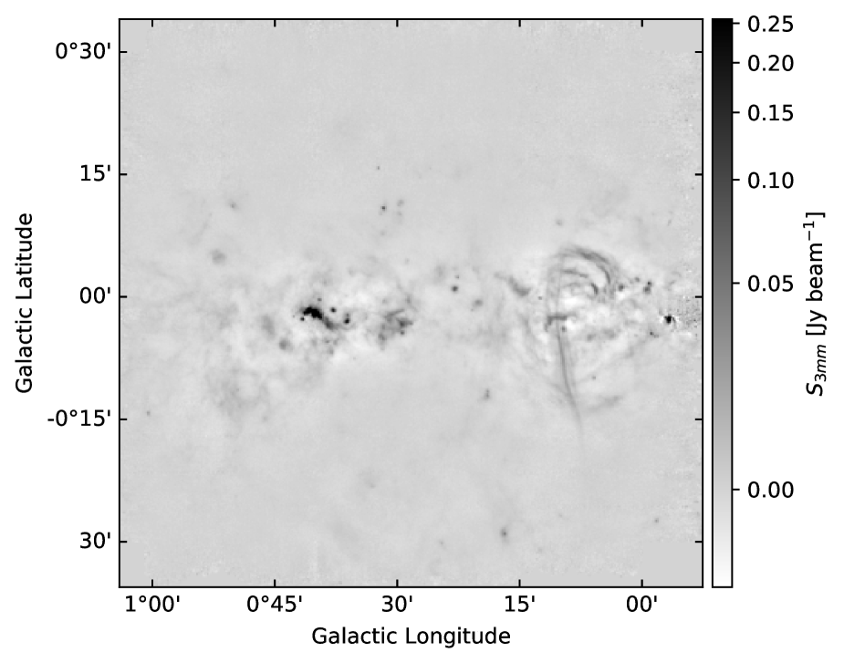
Figure 2: MUSTANG-2 image of the G01 field, centered on Sgr B2.

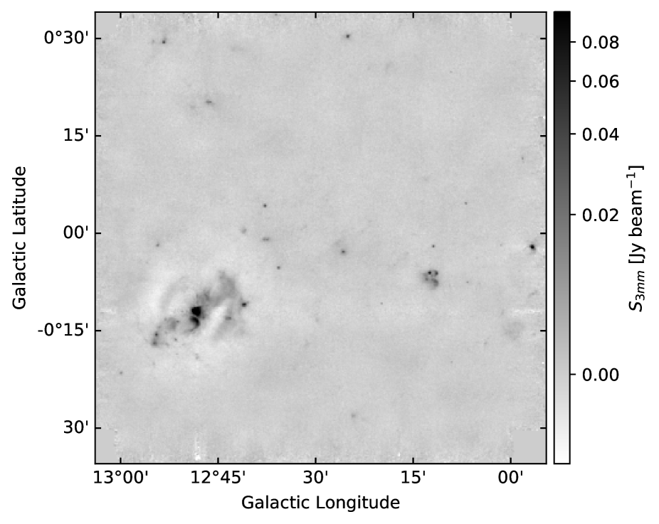
Figure 3: MUSTANG-2 image of the G12 field, including the W33 star-forming region.

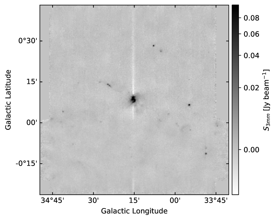
Figure 6: MUSTANG-2 image of the G34 field. Above $b\gtrsim 0\deg$, horizontal cross-scans have not been obtained; the vertical streak seen at $\ell=34.25\deg$ is a consequence of these missing data.

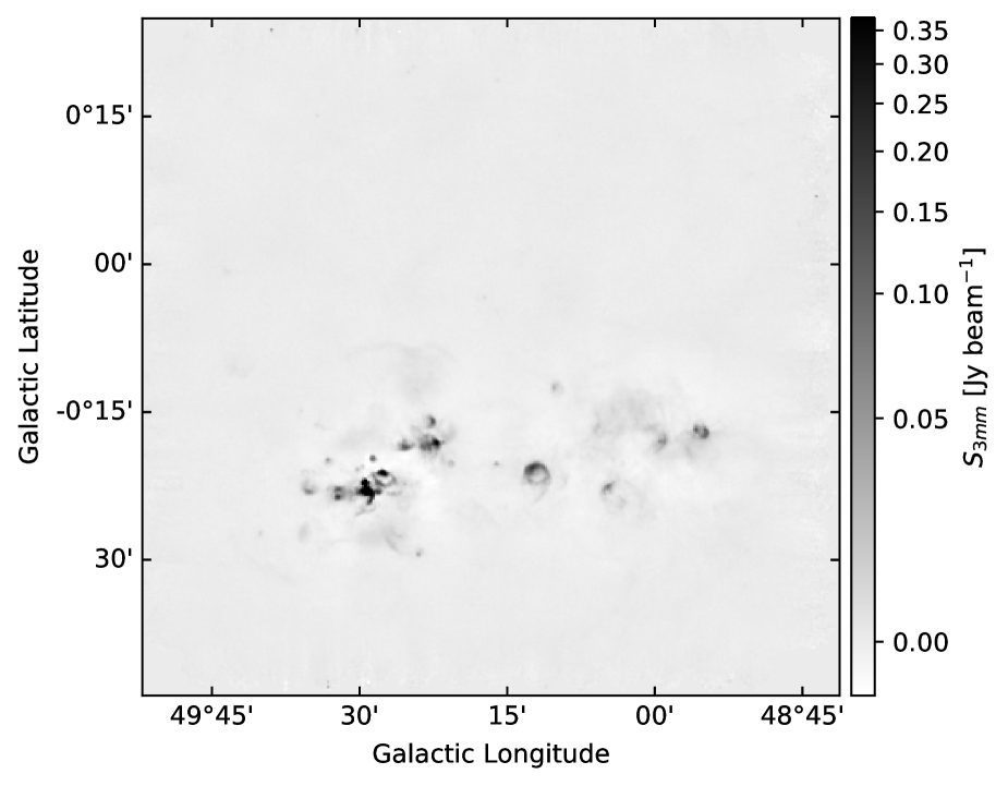
Figure 8: MUSTANG-2 image of the G49 field, which contains the W51 star-forming complex.

The processed images are shown in figures 2-8.

2.3 Sensitivity and beam size

The effective beam size in the delivered maps is the convolution of the intrinsic FWHM = 8.1″ beam with a FWHM = 4″ Gaussian kernel, resulting in a 9″ beam. This smoothing suppresses sub-beam-scale noise at a modest cost in beam area. The errors per beam reported in Table 2 correspond to these smoothed images.

2.4 Pointing Accuracy

Several corrections to the raw timestream data were required to produce maps. Individual scans were noted to have point sources shifted by up to half a beam ($\sim 4\arcsec$), indicating a timing error between the MUSTANG-2 pointing data and the true telescope pointing. To ensure that point sources were coincident in the maps, scans were cross-correlated with a first-iteration map, then assigned a new timing offset. The timing errors ranged from $\sim 10$ to $30$ milliseconds, corresponding to angular scales of $\approx 1-3\arcsec$ at our scan rate of $\approx 90$ arcseconds/second (scan speeds vary during an observation). Additional half-beam timing-related pointing errors were noted in some individual scans, resulting in additional streaking artifacts in the data. Most of these issues disappeared after smoothing the data with the 4″ kernel.

We compared the MUSTANG-2 maps with 20 cm images from the MAGPIS Galactic Plane survey (Helfand et al., 2006) and from other sources (Mehringer, 1994; Yusef-Zadeh et al., 2004) to measure pointing offsets, since these images showed the closest morphological match to the MGPS90 data. However, there are substantial regions in each field, particularly the Galactic center, that are synchrotron-dominated at 20 cm and have no corresponding features at 3 mm; we masked out these features. We use the image-registration toolkit to cross-correlate the MUSTANG-2 images with the 20 cm images and use a Fourier-domain upsampling approach to obtain sub-pixel positional offsets. We were not able to measure statistical uncertainties on these offsets, but correcting the images for the offsets resulted in smaller visual residuals in the difference images shown in Section 4. The measured offsets are reported in Table 2 and show the offset of the 20 cm data with respect to the MUSTANG-2 data. The mean and standard deviation offset from the 20 cm data are $\Delta\ell=1.8\pm 2\arcsec$ and $\Delta b=4.4\pm 2.7\arcsec$, respectively.

In several cases, the measured offset is comparable to the MUSTANG-2 beam. We therefore correct these images for the offset, assuming the VLA 20 cm data have correct pointing. The original pointing centers are recorded in the FITS headers of the published images with names CRVALnA so that the original pointing centers can be used if needed.

2.5 Effective Central Frequency

The MUSTANG-2 bandpass filter is approximately flat over the range 75 to 105 GHz, though including surface inaccuracies via the Ruze formula, the effective sensitivity declines by about a factor of three over this range. We multiplied the bandpass filter by power law flux density distributions with $S_{\nu}\propto\nu^{\alpha}$ to obtain the true effective central frequency of the bandpass for these assumed continuous distributions. They are reported in Table 3.

Table 3: Central Frequencies

$\alpha$	Frequency	Wavelength
	(GHz)	(mm)
0.0	87.85 GHz	3.413 mm
0.5	88.23 GHz	3.398 mm
1.0	88.62 GHz	3.383 mm
1.5	89.02 GHz	3.368 mm
2.0	89.41 GHz	3.353 mm
2.5	89.80 GHz	3.338 mm
3.0	90.19 GHz	3.324 mm
3.5	90.58 GHz	3.310 mm
4.0	90.96 GHz	3.296 mm

The central frequencies are computed by integrating the first moment of a power-law source function $S(\nu)=\nu^{\alpha}$ over the MUSTANG-2 bandpass including the effect of surface errors using the Ruze formula with an RMS surface accuracy 230 $\mu\textrm{m}$ (Frayer et al., 2018).

2.6 Combination with Planck data

The largest angular scale recovered by the MUSTANG-2 data pipeline is approximately 4.25′. Large angular scale structure is therefore missing. To recover those missing scales, we combine the MUSTANG-2 data with Planck 100 GHz data (with an effective central frequency of 104.225 GHz assuming a spectral index $\alpha=3$) scaled to an adopted central frequency of 90.19 GHz for MUSTANG-2, as appropriate for $\alpha=3$ (see Section 2.5). We use a simple feather procedure (Cotton, 2017) as implemented in the uvcombine python package. Planck’s spatial resolution is $\approx 10\arcmin$, substantially larger than the largest scale recovered in the MGPS data, so intermediate-scale structures (4-10′) are likely recovered poorly. These data are not used in the analysis in this paper, but the FITS images are provided in the data repository.

3 Compact Source Catalogs

We use astrodendro via the dendrocat wrapper to extract a catalog of compact structures. In brief, astrodendro catalogs hierarchically nested signal, effectively cataloging contoured regions. For the catalog described here, we included only the most compact structures, which are the ‘leaves’ in the catalog hierarchy.

To select primarily robust compact sources, we filter the images to reject scales $>45\arcsec$ prior to cataloging. We use a $4\sigma$ flux threshold and minimum of 100 pixels as the dendrogram parameters; the pixel scale is 1$\arcsec$/pixel, so our minimum object size is $\sim 1/2$ of beam area. We then reject sources with a peak signal-to-noise ratio less than 5, where we used the average noise level across the field. We report the noise level estimated using the median absolute deviation scaled to the standard deviation for each field in table 2.

The resulting catalog includes all of the significant pointlike sources in each field of view. However, this catalog also includes components of extended emission that had peaks that met the threshold criteria but are not distinct sources. The extended objects are a particularly prominent component of the Galactic center field.

To eliminate some of the extended structures, we then fit Gaussian profiles to each of the dendrogram-identified sources using the gaussfit_catalog package. Profiles were fitted to the original, unfiltered data. Profiles were restricted to have major and minor axes FWHM$<27\arcsec$, restricting the fits to be within a factor of three of the beam size. Sources substantially larger than this likely have measured integrated intensities attenuated by the filter function of the data acquisition and reduction pipeline; however, the full spatial transfer function of MUSTANG-2 has not yet been measured. Fits were performed to a 30″ radius around each source. If a second source was present in that radius, it was masked out with a single-beam-FWHM circle.

A total of 709 sources were identified across the seven fields. Of these, the majority, 385 were extended and round ($\sigma_{maj}>14\arcsec$), and an additional 251 had both long aspect ratios $\sigma_{maj}/\sigma_{min}>1.5$ and were extended ($\sigma_{maj}>14\arcsec$). Only 73 sources were compact ($\sigma_{maj}<14\arcsec$). Note that any confused or clustered sources, e.g., two compact sources within $\sim 5-20\arcsec$ of one another, would likely be classified as extended.

The full catalog is available on the project source code repository. A complete description of the catalog columns and an excerpt from the catalog are both shown in Appendix B.

3.1 Catalog cross-matching

We cross-match the resulting catalog with the catalogs listed in Table 4. Matches in these catalogs are included if there is a source within 10″ (approximately the MUSTANG-2 beam FWHM) of the MGPS catalog entry.

Table 4: Comparison Data Set Summary

Name	Wavelength(s)	Angular Resolution	Approximate Sensitivity∗	References
	$\mu\textrm{m}$	″	mJy $\textrm{beam}^{-1}$
Spitzer GLIMPSE	3.6–8.0	2	-	Churchwell et al. (2009)
Spitzer MIPSGAL	24	6	-	Gutermuth & Heyer (2015)
Herschel Hi-GAL	70–500	6–36	20-85	Molinari et al. (2016); Elia et al. (2017)
APEX-Laboca ATLASGAL	870	20	70	Urquhart et al. (2014)
CSO-Bolocam BGPS	1100	33	50	Rosolowsky et al. (2010)
				Ginsburg et al. (2013)
GBT-MUSTANG-2 MGPS90	3274	9	1-2	This work
	cm
MAGPIS	6	4	2.5	Giveon et al. (2005a)
				Helfand et al. (2006)
CORNISH	6	1.5	2.5	Hoare et al. (2012)
MAGPIS	20	5	2	Giveon et al. (2005b)

^∗ When no matching entry was found, we adopted the listed value as a $1-\sigma$ upper limit on the source flux when plotting SEDs. However, all of these surveys have significantly varying point source sensitivity at different locations, so these limits should be treated as very loose. The GLIMPSE and MIPSGAL catalog data were not cross-matched, so no upper limit was used in SED fitting, but we used images from these surveys to produce cutout images for morphological comparison (see Figures 9 to 11). The Hi-GAL sensitivity and angular resolution values both rise from 70 to 500 $\mu\textrm{m}$. Note that the PACS 70$\mu\textrm{m}$ beam in the Hi-Gal data set is asymmetric, $\sim 6\times 12\arcsec$ (Molinari et al., 2016).

Of the 709 total MGPS90 sources, 279 passed our selection criteria that the peak signal-to-noise ratio in the source was $SNR>5$ and the peak signal was at least twice that of the background, $S_{peak}>2S_{background}$.. Of those, 240 had millimeter/submillimeter matches (Herschel 70-500 $\mu\textrm{m}$, LABOCA 870 $\mu\textrm{m}$, or Bolocam 1.1 mm), 119 had centimeter-wavelength matches (6 cm or 20 cm), and 34 had no match in the millimeter or centimeter catalogs. There were 126 sources cross-matched at shorter wavelengths but not at longer wavelengths, and 5 with long-wavelength matches but no short-wavelength.

Figure 1 shows the histogram of MUSTANG-2-measured fluxes in the catalog. Because the typical noise level was $\sim 1$ mJy, the catalog has few sources below 5 mJy. The overlaid histogram shows the subset of the sample with no detections at other wavelengths; this subset is much fainter than the overall distribution, suggesting that the majority of these sources were either below the detection limit or the confusion limit of the other surveys.

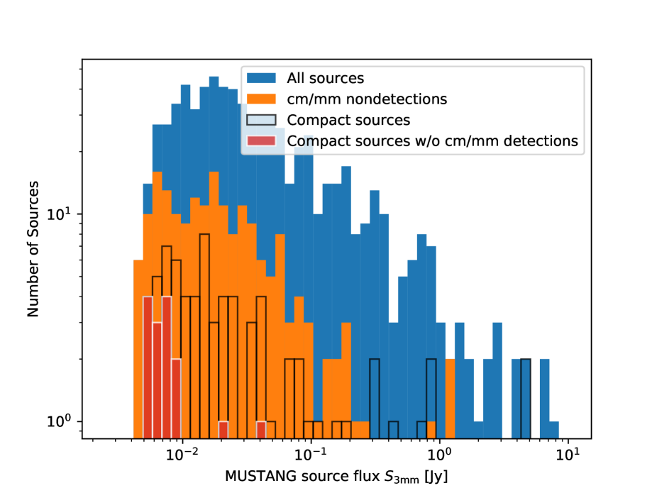
Figure 1: Histogram of the source catalog. Blue shows all sources, while orange (overlaid as a foreground layer) shows only those sources that have no matches at cm or mm wavelengths in the searched surveys.

3.2 HCH ii region identification

One of the aims of this survey is to identify the youngest high-mass protostars. Candidates are those sources with little to no mid-infrared emission and very compact, optically thick (hypercompact) H ii regions.

Massive stars form in the middle of ultra-dense cores undergoing gravitational collapse, leading to an accretion rate of order $\dot{M}\sim 10^{-3}$ $M_{\odot}$ $\textrm{yr}^{-1}$ such that a 100 $M_{\odot}$ star takes about $10^{5}$ years to accrete its mass. As the star contracts onto the main sequence it starts to ionize its environment to create an HCH ii region. For a sufficiently dense accretion flow, the Strömgren radius of the HCH ii region is bound by the gravity of the star, with a radius $R_{G}\sim$50-100 AU (Keto, 2002, 2003, 2007). Such gravitationally bound HCH ii regions are optically thick at centimeter wavelengths and therefore emit as blackbodies at wavelengths $\lambda\gtrsim$3 mm, with

$$S_{\nu}=21~{}\textrm{mJy}\left(\frac{d}{5~{}\textrm{kpc}}\right)^{-2}\left(\frac{R}{100~{}\textrm{AU}}\right)^{2}\left(\frac{\nu}{90~{}\textrm{GHz}}\right)^{2}$$ (2)

which is only 0.06 mJy at $\nu=5$ GHz, and therefore below the detection limit of many existing surveys; they are certainly unremarkable sources at long wavelengths. HCH ii regions can be distinguished from older ultracompact (UCH ii) regions by their bright 90 GHz emission and faint emission at 5 GHz and lower frequencies. Sources with free-free emission that peaks at or just below 3 mm represent the youngest high-mass YSOs. The dense cores surrounding these sources will be bright in the millimeter regime, since they will have high dust column densities and temperatures.

We therefore select candidate HCH ii regions as those fitting either of these criteria:

1. $S_{3\mathrm{mm}}>1.75~{}S_{6\mathrm{cm}}$. This requirement selects free-free sources that have $\tau_{\textit{ff}}=1$ at ${\lambda={6~{}\mathrm{cm}}}$. It corresponds to an emission measure ${EM=7\times 10^{7}~{}\mathrm{cm}^{-6}~{}\mathrm{pc}}$.

2. The source is not detected at 6 and 20 cm, is detected at 1.1 mm, and has

   $$\frac{S_{3\mathrm{mm}}}{S_{1.1\mathrm{mm}}}>\left(\frac{3.28~{}\mathrm{mm}}{1.11~{}\mathrm{mm}}\right)^{-\alpha}=0.039$$ (3)

   
   

   where $\alpha=3$ is the spectral index for optically thin dust with an opacity index $\beta=1$. This requirement selects dust-detected sources in which there is some indication of an excess of free-free emission over pure dust emission at 3 mm. HCH ii regions that are optically thick up to $\sim 3$ mm, those that are extremely compact and dense, are below the detection threshold of the centimeter surveys ($\approx 2.5$ mJy at 6 cm; Giveon et al., 2005a; Hoare et al., 2012).

These criteria provide a small sample of 5 candidate HCH ii regions across the seven target regions. Only 3 of these candidates were morphologically compact. This sample consists of known ultracompact or HCH ii region clusters (three are parts of W49A, which contains 12 sources that can be classified as HCH ii regions; De Pree et al., 1997), the HCH ii region G34.257+0.153, and the OH/IR star G30.944+0.035 (Wilson & Barrett, 1972). The ten known HCH ii regions in W51 (Ginsburg et al., 2016a) were not recovered because they are blended, in the 9″ MUSTANG-2 beams, with more diffuse H ii regions.

However, the majority of sources in our catalog do not have centimeter-wavelength detections and therefore were not eligible to be selected based on criterion 1 above. The BGPS 1.1 mm data, which have only 30″ resolution, could be affected by confusion (source blending) and therefore be too bright for a 3 mm excess to be detected, preventing selection by criterion 2.

While we would expect some free-free excess at 90 GHz above the dust emission extrapolated from 1.1 mm in dusty HCH ii regions, it is plausible that the excess is not enough to modify the spectral index to meet our selection criterion 2. Sources that have millimeter detections (since they must be surrounded by gas and dust) and not centimeter detections therefore remain candidate HCH ii regions. This large sample of 126 additional candidates, especially the 10 that are compact, are interesting candidates for future deep centimeter observations.

Several well-known HCH ii regions were excluded from these selection criteria. The HCH ii regions in W51, including the W51e cluster and W51d2 (Ginsburg et al., 2016b), those in W49 (De Pree et al., 1997), and those in Sgr B2 (De Pree et al., 1998) are confused, residing in the same beams as other high-mass stars at different evolutionary states. G34.257+0.153 includes a pair of HCH ii regions but less other surrounding emission, so it did pass our selection criteria (Sewilo et al., 2004; Avalos et al., 2006). MGPS90 is clearly capable of detecting HCH ii regions that are not in dense protoclusters.

3.3 Constraints on HCH ii lifetimes

To estimate the relative lifetime of the hypercompact and ultracompact phases, we compare the number of HCH ii candidates to the number of detected UCH ii regions from the CORNISH survey (Kalcheva et al., 2018). Wood & Churchwell (1989b) seeded the idea that UCH ii lifetimes may be substantially longer than expected for a freely expanding Strömgren sphere $t_{\textrm{fe}}\sim 4\times 10^{4}$ years, but the improved sample of Kalcheva et al. (2018) suggests that the discrepancy is not so large. In any case, we adopt a loosely estimated UCH ii lifetime within the range $4\times 10^{4}~{}\mathrm{yr}<t_{\textup{UCH\,{ii}}}<4\times 10^{5}~{}\mathrm{yr}$.

In the observed regions, the CORNISH survey detected 73 UCH ii regions. Over the same area, our sample includes 10 compact MUSTANG-2 sources with no centimeter detections, which are our additional candidates from §3.2, and four previously-known HCH ii regions. W51 contains 10 and W49A contains up to 12 additional HCH ii region candidates when viewed at high resolution (De Pree et al., 1997; Ginsburg et al., 2016b). The inferred lifetime of HCH ii regions, using a sample size of 12-34 HCH ii’s in the MGPS90 fields, is therefore $16-46\%$ that of UCH ii regions, or $6\times 10^{3}\mathrm{yr}<t_{\textup{HCH\,{ii}}}<2\times 10^{5}\mathrm{yr}$. A more complete assessment from the larger survey may more tightly constrain these values.

Furthermore, though, the relatively small number of new candidates (only 10) compared to the large numbers in compact regions suggests that HCH ii regions form primarily in, or live longest in, clustered regions. This high production of HCH ii regions in dense protoclusters can be either because more high-mass stars form there, indicating an overall higher population, or because the gas density is higher, allowing the H ii regions to remain in the hypercompact phase for a longer period before expanding into UCH ii or diffuse H ii regions.

Figure 4: MUSTANG-2 image of the G29 field.

Figure 5: MUSTANG-2 image of the G31 field containing W43.

Figure 7: MUSTANG-2 image of the G43 field, which contains the W49A star-forming complex (center) and the W49B supernova remnant (just southeast of center).

3.4 Representative SEDs of selected sources

To put the MGPS90 data in context, we show a few examples of SEDs extracted from the catalogs described in section 3.1 along with cutout images extracted from the same surveys. The SEDs include the catalog-reported flux values from each of the cross-matched surveys and the dendrogram source flux for MUSTANG. The selected SEDs are of a probable planetary nebula (Fig. 9), which exhibits emission at all wavelengths and was detected in extended $H-\alpha$ emission (Sabin et al., 2014), an OH/IR star (Fig. 12) that is infrared- and millimeter-bright but not detected at centimeter wavelengths, a high-mass YSO that is a candidate HCH ii region with no centimeter detection (Fig. 10), and a source containing a known pair of HCH ii regions (Fig. 11). These SEDs highlight the important role of MGPS90 data in bridging the gap between the millimeter and centimeter regimes.

Figure 9: SED of source G29.578-0.268, a candidate planetary nebula. The individual panels show cutouts from various surveys hosted on the MAGPIS cutout service (https://third.ucllnl.org/gps/) and the Herschel Hi-GAL cutout service (https://tools.ssdc.asi.it/HiGAL.jsp); individual survey references are in Section 3.1. The white bar in the lower-left is a 1′ scalebar. Short wavelengths ($<24$ $\mu\textrm{m}$) are not included in the SED, the rest are included in the cross-matched catalog.

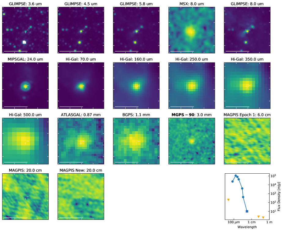
Figure 10: SED of source G12.026-0.031, a candidate HCH ii region and likely high-mass YSO identified in the RMS survey (Lumsden et al., 2013). This compact source failed the criteria in Section 3.2, indicating that no clear excess of free-free emission is detected at 3 mm, and suggesting that if an HCH ii region is present, it is faint. Such objects are of particular interest because they constitute the most compact and likely youngest forming high-mass stars.

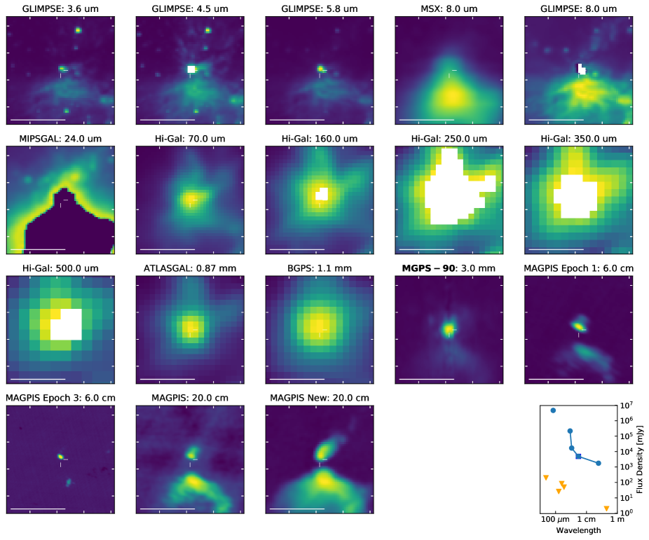
Figure 11: SED of source G34.257+0.153, which contains several HCH ii regions within the MGPS90 beam (Avalos et al., 2009; Sewiło et al., 2011). The source passed the selection criteria in Section 3.2, confirming that these are useful criteria for identifying relatively isolated HCH ii regions. The intermediate Herschel wavelengths (160, 250, 350 $\mu\textrm{m}$) appear as upper limits though the source is saturated in these Hi-Gal bands; these data points should be ignored. The asymmetry in the MGPS90 image is caused by the missing scans noted in Figure 6.

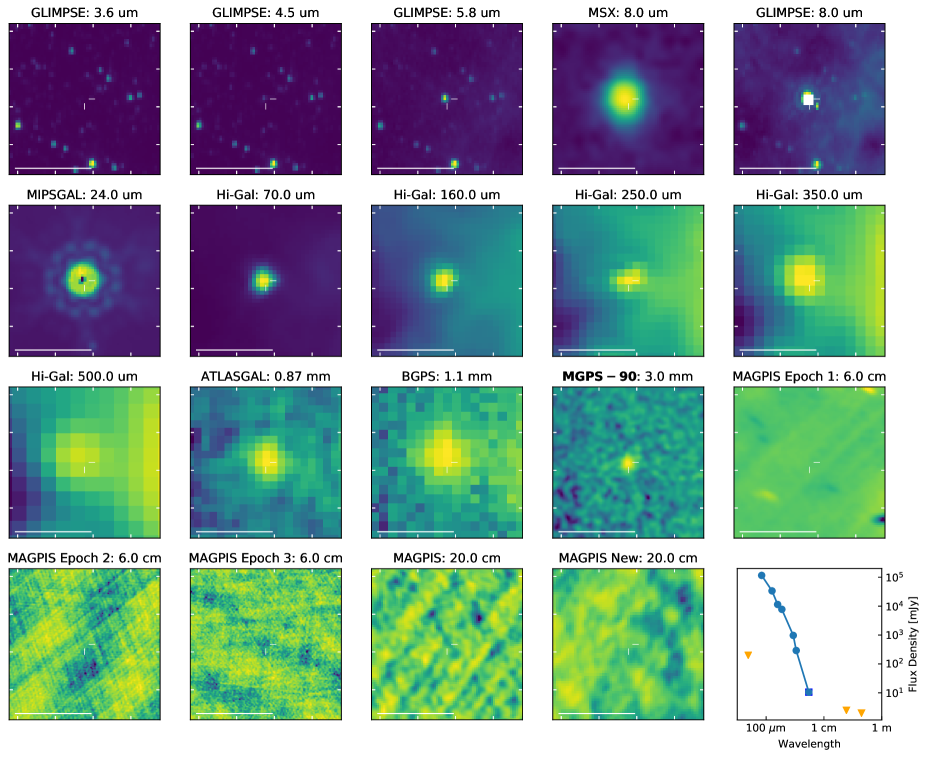
Figure 12: SED of source G30.944+0.035, an OH/IR star. The dusty SED with no detected radio emission made this source a candidate hypercompact HII region based on the criteria in Section 3.2, though it only barely passed the second criterion.

4 Diffuse Emission: Free-free separation

As stated in the introduction, the MGPS90 data have contributions from thermal free-free, thermal dust continuum, and nonthermal synchrotron emission. We describe here our decomposition of the MGPS90 data into free-free and dust emission; the non-thermal emission was not separated from the free-free emission.

We use the ATLASGAL 870 $\mu$m data (Schuller et al., 2009) to estimate the dust contribution since at 870 $\mu$m essentially all emission is from dust. We estimate the 90 GHz flux density from dust by scaling the ATLASGAL data assuming a dust emissivity index $\beta=1.5$. Using this value of $\beta$, the ATLASGAL 870 $\mu$m and MGPS90 data flux densities are related via $S_{\rm 90GHz}\simeq 0.013~{}S_{\rm 870\mu m}$ (cf. Equation 1). Values of $\beta$ ranging from $1<\beta<2$ are often inferred from SED modeling, so there is substantial (factor of $\sim 4$) uncertainty in the extrapolated dust fluxes. While this uncertainty limits our ability to quantitatively interpret the dust-subtracted images, the morphology of these images is less affected. We subtract the scaled ATLASGAL data from an appropriately smoothed version of the MGPS90 map to obtain an estimated free-free map. We perform this subtraction on the feathered MGPS90 and Planck data (Section 2.6).

Similarly, we use 20 cm maps to estimate the dust contribution by subtracting a scaled 20 cm map from the MGPS90 data. For most fields, we use 20 cm MAGPIS data (Helfand et al., 2006), which has an angular resolution of $\sim\!6\arcsec$ and a point source sensitivity of $1-2$ mJy. MAGPIS does not cover the Galactic center or $\ell>48^{\circ}$, and so we use other data in these zones. In the Galactic center, we use the multi-configuration 20 cm map from Yusef-Zadeh et al. (2004, resolution $\sim 30\arcsec$), and in the W51 field we use the multi-configuration map from Mehringer (1994, resolution $\lesssim 1\arcsec$). We scale the 20 cm to 90 GHz assuming the 20 cm consists exclusively of optically thin free-free emission following a power law $S_{\nu}\propto\nu^{-0.12}$ (Wilson et al., 2009). The observed fields were selected based on their rich ongoing star formation activity, so this approximation is reasonable, but there are several cases where additional emission mechanisms (e.g., synchrotron) contribute to the observed intensity.

We show the results of the decomposition for one example field in Figure 13; the rest of the MGPS90 fields are in the Appendix. Figure 13 contains panels of the MGPS90 data, the contribution to the MGPS90 data from thermal dust estimated from ATLASGAL subtraction, the contribution to the MGPS90 data from free-free and synchrotron emission, 20 cm data, and the contribution to the MGPS90 data from thermal dust estimated from 20 cm subtraction.

The example in Figure 13 shows good agreement between the two dust estimates and between the free-free estimates, and the differences highlight some of the incorrect assumptions in the above analysis. The excess diffuse emission in the rightmost panel (MGPS90 - VLA) is most likely caused by the VLA’s failure to recover large angular scales. The missing emission on the right side of that map is caused by the excess synchrotron emission in the Sgr A region, which is not accounted for in our simple free-free model. Both dust maps do well at recovering emission from the massive G0.253+0.015 cloud (the bean-shaped feature in the upper left) and the southern dust ridge (the prominent dust feature just below the center of the map).

The W43 region is substantially more dust-dominated than the Galactic Center (Figure 14). The dusty features, however, are all closely aligned with free-free features, so it is difficult to disentangle them by eye in the MGPS90 image. The MGPS90 - 20 cm image is negative in the 20 cm-dominated regions, likely indicating that there is substantial nonthermal emission in these HII regions. While there are no known supernovae in the region, the population of OB and Wolf-Rayet stars powering the expanding HII region may also drive strong shocks into the surrounding medium (e.g. Bally et al., 2010), leading to nonthermal emission. The presence of such nonthermal emission indicates that electrons must be accelerated to relativistic velocities in the HII region, which has recently been shown to be possible in HII region expansion fronts (Padovani et al., 2019).

The W49B supernova remnant in the G43 field stands out as a bright nonthermal source. No other supernova remnants in the surveyed area are as bright at 3 mm (see Figure 7). Sun et al. (2011) found that the spectral energy distribution of W49B is well-fit by a single power law from 200 MHz to 30 GHz with index $\alpha=-0.46\pm 0.01$. They found that the 5 GHz integrated flux density is $19.10\pm 0.98$ Jy, and the 90 GHz integrated flux density should be 5.1 Jy. Integrating over W9B, we find a flux density of 5.2 Jy, indicating that most of the associated emission is nonthermal.

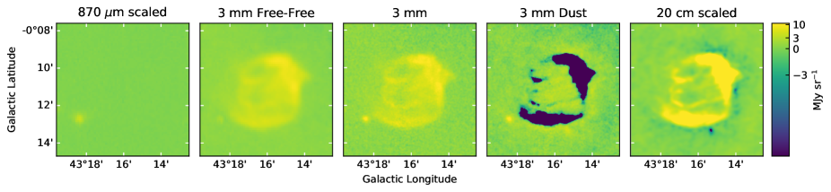
Figure 20: Decomposition of the MGPS90 data in the G43 field centered on W49B. See Figure 13 for a description of the panels. W49B is a supernova remnant completely dominated by synchrotron emission. Panel (b) therefore shows synchrotron, not free-free, emission.

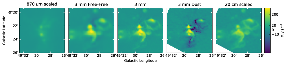
Figure 21: Decomposition of the MGPS90 data in the G49 field centered on W51 Main. See Figure 13 for a description of the panels. There is a mix of under- and over-subtracted emission in the dust map in panel (d); the arc shape in the center is purely free-free emission (Ginsburg et al., 2016b, 2017), but it is optically thick at 20 cm.

The decomposed images are shown in Figures 13-21.

Table 5: Free-free and Dust Emission Fractions

Field Name	Center (Galactic)	Field Size	Dust Fraction ($\beta=1.5$)
	degrees	arcminutes
Arches	0.140 -0.054	12.60	0.08
Sgr B2	0.657 -0.041	12.80	0.13
W33	12.805 -0.206	3.72	0.11
G29	29.927 -0.041	5.87	0.11
W43	30.757 -0.045	7.24	0.10
G34	34.257 0.148	2.80	0.21
W49a	43.171 -0.006	4.38	0.13
W49b	43.268 -0.186	3.53	0.04
W51a	49.461 -0.368	8.75	0.14
W51b	49.080 -0.338	11.30	0.07

We directly quantify the dust contribution to the 3 mm intensity in the targeted brightest fields. Each field includes one or more prominent extended structures that were the focus for these pilot observations. For each of these structures, we extracted an area that encompasses the bulk of the 3 mm emission and measured the fraction of that emission that is explained by optically-thin dust, which is the sum of the positive values from the scaled ATLASGAL data explained above divided by the sum of the 3 mm emission. The results are reported in Table 5. Because we have assumed $\beta=1.5$, and typical dust $\beta$ values for the ISM are $\sim 1.5-2$ (e.g., Ossenkopf & Henning, 1994), these can be treated as upper limits on the dust contribution.

In the regions of interest, the dust contribution at 3 mm is limited to $\lesssim 20\%$ on the several arcminute scales probed. Regions with substantial synchrotron contributions from supernova remnants (W49b, W51b) or other mechanisms (the Arches) have an even lower contribution from dust, $<10\%$. In short, the integrated diffuse emission detected in MGPS90 is dominated by emission from hot gas rather than from cold molecular gas. We are, however, unable to determine whether the area of the survey is dominated by hot or cold gas, as the large angular scale filtering of the interferometric data sets prevents such an assessment; it remains possible that the area (and volume) of the surveyed regions is dominated by cold dust emission, while the received flux is clearly dominated by hot gas.

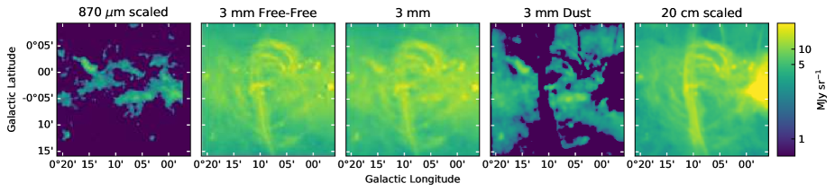
Figure 13: Decomposition of the MGPS90 data in the G01 field centered on the Arches region. All images are displayed on the same intensity scale. In the G01 field, the 20 cm data have 30″ resolution, so the MGPS90 data have been smoothed to match the resolution of the other images. From left to right, (a; 870 $\mu\textrm{m}$ scaled) ATLASGAL 870 $\mu\textrm{m}$ scaled to 3 mm, (b; 3 mm free-free) smoothed MGPS90 - scaled ATLASGAL, (c; 3 mm) MGPS90, (d; 3 mm Dust) smoothed MGPS90 - scaled VLA 20 cm continuum, (e; 20 cm scaled) VLA 20 cm continuum scaled to 3 mm. The images are displayed with a logarithmic stretch.

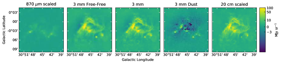
Figure 14: Decomposition of the MGPS90 data in the G31 field centered on W43. See Figure 13 for a description of the panels. In G31, the 20 cm data have $\sim 5$ ″ resolution, so they are smoothed to match the MGPS90 data to create panels (d) and (e), while the MGPS90 data are smoothed to match the ATLASGAL data to create panel (b).

5 Conclusions

We have presented the pilot data for the MUSTANG 90 GHz Galactic Plane Survey, MGPS90. When complete, this survey will cover most of the northern Galactic plane within $|b|<0.5^{\circ}$. These initial data cover several high-mass star cluster forming regions. All imaged regions are dominated by free-free and synchrotron emission at 3 mm.

We cataloged emission in the images, identifying 279 sources using the dendrogram algorithm, of which 3 are verified HCH ii regions, and another 10 are plausible candidates.

Appendix A Additional free-free / dust decomposition maps

In this appendix, we show cutout images focused on a selection of bright extended emission regions and the associated free-free decomposition described in Section 4.

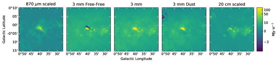
Figure 15: Decomposition of the MGPS90 data in the G01 field centered on Sgr B2. See Figure 13. The differences in the ATLASGAL- and 20 cm-based dust decomposition highlight the different angular scales recovered by those data sets.

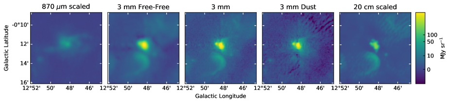
Figure 16: Decomposition of the MGPS90 data in the G12 field centered on W33. See Figure 13 for a description of the panels. The diffuse free-free emission is well-removed by subtracting the 20 cm data, but the compact point source appears much brighter in the 3 mm-derived map; this difference is likely because free-free emission is present but optically thick at 20 cm, resulting in an underestimate of the free-free contribution at 3 mm.

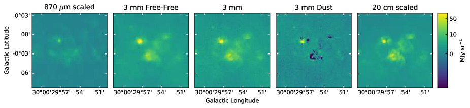
Figure 17: Decomposition of the MGPS90 data in the G29 field. See Figure 13 for a description of the panels. Some of the compact structures exhibit strong excesses at 20 cm.

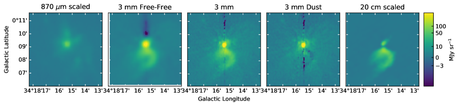
Figure 18: Decomposition of the MGPS90 data in the G34 field centered on G34.26+0.15. See Figure 13 for a description of the panels. The vertical streak is an artifact as mentioned in Figure 6.

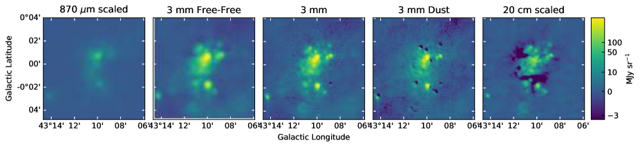
Figure 19: Decomposition of the MGPS90 data in the G43 field centered on W49A. See Figure 13 for a description of the panels. As in Figure 17, several compact structures appear to have excess 20 cm emission. However, other structures exhibit free-free emission that is optically thick at 20 cm and is therefore under-subtracted at 3 mm in panel (d); see also Figure 21.

Appendix B Catalog

Table 6 shows an excerpt from the catalog including the brightest 20 sources. The full catalog will be published electronically with the paper. We include the dendrogram measurements of the integrated flux density and the Galactic $\ell$ and $b$ centroids, integrated flux densities in 10″ and 15″ apertures, the median background in a 15-20″ aperture, and the parameters of the best-fit two-dimensional Gaussian profile. The sample table is sorted by the Gaussian peak amplitude ($A_{G}$) in descending order.

Table 6: MUSTANG-2 Source IDs and photometry

ID	Dendrogram $S_{\nu}$	$\ell$	$b$	$S_{\nu,10^{\prime\prime}}$	$S_{\nu,15^{\prime\prime}}$	$S_{bg;15-20^{\prime\prime}}$	$A_{G}$	$\ell_{G}$	$b_{G}$	FWHMmaj,G	FWHMmin,G	PAG
	$\mathrm{Jy}$	∘	∘	$\mathrm{Jy}$	$\mathrm{Jy}$	$\mathrm{Jy\,beam^{-1}}$	$\mathrm{Jy\,beam^{-1}}$	∘	∘	′′	′′	∘
35.00	17.01	12.805	-0.201	3.657	6.887	2.292	5.80	12.806	-0.201	17.034	14.966	90
56.00	8.30	43.167	0.010	3.099	5.49	1.564	5.22	43.167	0.010	15.685	11.546	76.062
166.00	12.58	0.668	-0.035	2.699	5.067	1.846	3.94	0.668	-0.036	16.34	15.036	343.275
14.00	4.88	34.257	0.153	2.333	3.728	0.592	4.56	34.257	0.153	11.208	9.439	67.04
66.00	6.43	49.492	-0.368	2.071	3.644	1.059	3.10	49.492	-0.368	16.674	13.335	132.052
49.00	11.59	49.489	-0.380	1.698	3.408	1.481	2.06	49.488	-0.380	21.262	14.499	141.889
42.00	4.67	43.166	-0.030	1.394	2.501	0.773	2.33	43.166	-0.030	13.947	13.589	360
142.00	4.16	359.946	-0.046	0.853	1.604	0.624	1.42	359.946	-0.046	14.779	14.363	360
116.00	2.70	29.957	-0.017	0.766	1.451	0.409	1.37	29.956	-0.017	14.89	12.647	65.432
36.00	0.95	12.813	-0.199	0.692	1.19	0.345	1.15	12.812	-0.199	27.0	21.545	360
41.00	2.64	29.957	-0.018	0.653	1.204	0.402	1.06	29.957	-0.018	15.584	14.434	0
45.00	1.40	49.491	-0.386	0.602	1.175	0.428	0.74	49.491	-0.386	27.0	19.286	256.306
51.00	0.69	43.172	-0.001	0.448	0.82	0.251	0.70	43.172	-0.000	16.815	15.165	360
179.00	1.32	31.412	0.308	0.374	0.696	0.201	0.61	31.412	0.307	15.161	13.027	121.242
164.00	0.83	30.866	0.114	0.372	0.593	0.101	0.69	30.866	0.114	11.418	10.267	129.634
62.00	0.93	30.720	-0.083	0.362	0.617	0.136	0.68	30.720	-0.083	12.342	11.126	130.278
55.00	1.85	43.149	0.012	0.326	0.623	0.241	0.73	43.148	0.013	19.1	13.303	0
156.00	0.57	0.658	-0.042	0.261	0.447	0.109	0.48	0.659	-0.041	27.0	13.659	135.233
133.00	0.90	30.534	0.021	0.248	0.446	0.132	0.41	30.534	0.021	15.429	12.704	150.774

The subscripts X_G are for the parameters derived from Gaussian fits. The values displayed are rounded such that the error is in the last digit; error estimates can be found in the digital version of the table.Note that position angles in the set (0, 90, 180, 270, 360) are caused by bad fits. These fits are kept in the catalog because they passed other criteria and are high signal-to-noise, but they are likely of sources in crowded regions so the corresponding fit parameters should be treated with caution.

References

- Aguirre et al. (2011) Aguirre, J. E., Ginsburg, A. G., Dunham, M. K., et al. 2011, ApJS, 192, 4
- Avalos et al. (2009) Avalos, M., Lizano, S., Franco-Hernández, R., Rodríguez, L. F., & Moran, J. M. 2009, ApJ, 690, 1084
- Avalos et al. (2006) Avalos, M., Lizano, S., Rodríguez, L. F., Franco-Hernández, R., & Moran, J. M. 2006, ApJ, 641, 406
- Bally et al. (2010) Bally, J., Aguirre, J., Battersby, C., et al. 2010, ApJ, 721, 137
- Beuther et al. (2016) Beuther, H., Bihr, S., Rugel, M., et al. 2016, A&A, 595, A32
- Churchwell et al. (2009) Churchwell, E., Babler, B. L., Meade, M. R., et al. 2009, PASP, 121, 213
- Condon & Ransom (2007) Condon, J. J., & Ransom, S. 2007, Essential Radio Astronomy (NRAO). http://www.cv.nrao.edu/course/astr534/ERA.shtml
- Condon & Ransom (2016) Condon, J. J., & Ransom, S. M. 2016, Essential Radio Astronomy
- Cotton (2017) Cotton, W. D. 2017, PASP, 129, 094501
- Csengeri et al. (2014) Csengeri, T., Urquhart, J. S., Schuller, F., et al. 2014, A&A, 565, A75
- De Pree et al. (1998) De Pree, C. G., Goss, W. M., & Gaume, R. A. 1998, ApJ, 500, 847
- De Pree et al. (1997) De Pree, C. G., Mehringer, D. M., & Goss, W. M. 1997, ApJ, 482, 307
- Dicker et al. (2014) Dicker, S. R., Ade, P. A. R., Aguirre, J., et al. 2014, in Society of Photo-Optical Instrumentation Engineers (SPIE) Conference Series, Vol. 9153, Proc. SPIE, 91530J
- Dickinson et al. (2018) Dickinson, C., Ali-Haïmoud, Y., Barr, A., et al. 2018, New A Rev., 80, 1
- Dünner et al. (2013) Dünner, R., Hasselfield, M., Marriage, T. A., et al. 2013, ApJ, 762, 10
- Eden et al. (2017) Eden, D. J., Moore, T. J. T., Plume, R., et al. 2017, MNRAS, 469, 2163
- Elia et al. (2017) Elia, D., Molinari, S., Schisano, E., et al. 2017, MNRAS, 471, 100
- Fomalont et al. (2014) Fomalont, E., van Kempen, T., Kneissl, R., et al. 2014, The Messenger, 155, 19
- Frayer et al. (2018) Frayer, D. T., Ghigo, F., & Maddalena, R. J. 2018, arXiv e-prints, arXiv:1811.00105
- Galván-Madrid et al. (2009) Galván-Madrid, R., Keto, E., Zhang, Q., et al. 2009, ApJ, 706, 1036
- Ginsburg et al. (2013) Ginsburg, A., Glenn, J., Rosolowsky, E., et al. 2013, ApJS, 208, 14
- Ginsburg et al. (2016a) Ginsburg, A., Goss, W. M., Goddi, C., et al. 2016a, A&A, 595, A27
- Ginsburg et al. (2016b) Ginsburg, A., Henkel, C., Ao, Y., et al. 2016b, A&A, 586, A50
- Ginsburg et al. (2017) Ginsburg, A., Goddi, C., Kruijssen, J. M. D., et al. 2017, ApJ, 842, 92
- Giveon et al. (2005a) Giveon, U., Becker, R. H., Helfand, D. J., & White, R. L. 2005a, AJ, 129, 348
- Giveon et al. (2005b) —. 2005b, AJ, 130, 156
- Gutermuth & Heyer (2015) Gutermuth, R. A., & Heyer, M. 2015, AJ, 149, 64
- Helfand et al. (2006) Helfand, D. J., Becker, R. H., White, R. L., Fallon, A., & Tuttle, S. 2006, AJ, 131, 2525
- Hoare et al. (2012) Hoare, M. G., Purcell, C. R., Churchwell, E. B., et al. 2012, PASP, 124, 939
- Kalcheva et al. (2018) Kalcheva, I. E., Hoare, M. G., Urquhart, J. S., et al. 2018, A&A, 615, A103
- Keto (2002) Keto, E. 2002, ApJ, 580, 980
- Keto (2003) —. 2003, ApJ, 599, 1196
- Keto (2007) —. 2007, ApJ, 666, 976
- Lumsden et al. (2013) Lumsden, S. L., Hoare, M. G., Urquhart, J. S., et al. 2013, ApJS, 208, 11
- Medina et al. (2019) Medina, S. N. X., Urquhart, J. S., Dzib, S. A., et al. 2019, A&A, 627, A175
- Mehringer (1994) Mehringer, D. M. 1994, ApJS, 91, 713
- Molinari et al. (2010) Molinari, S., Swinyard, B., Bally, J., et al. 2010, A&A, 518, L100
- Molinari et al. (2016) Molinari, S., Schisano, E., Elia, D., et al. 2016, A&A, 591, A149
- Ossenkopf & Henning (1994) Ossenkopf, V., & Henning, T. 1994, A&A, 291, 943
- Padovani et al. (2019) Padovani, M., Marcowith, A., Sánchez-Monge, Á., Meng, F., & Schilke, P. 2019, A&A, 630, A72
- Romero et al. (2020) Romero, C. E., Sievers, J., Ghirardini, V., et al. 2020, ApJ, 891, 90
- Rosolowsky et al. (2010) Rosolowsky, E., Dunham, M. K., Ginsburg, A., et al. 2010, ApJS, 188, 123
- Sabin et al. (2014) Sabin, L., Parker, Q. A., Corradi, R. L. M., et al. 2014, MNRAS, 443, 3388
- Schuller et al. (2009) Schuller, F., Menten, K. M., Contreras, Y., et al. 2009, A&A, 504, 415
- Sewilo et al. (2004) Sewilo, M., Churchwell, E., Kurtz, S., Goss, W. M., & Hofner, P. 2004, ApJ, 605, 285
- Sewiło et al. (2011) Sewiło, M., Churchwell, E., Kurtz, S., Goss, W. M., & Hofner, P. 2011, ApJS, 194, 44
- Sun et al. (2011) Sun, X. H., Reich, P., Reich, W., et al. 2011, A&A, 536, A83
- Urquhart et al. (2014) Urquhart, J. S., Moore, T. J. T., Csengeri, T., et al. 2014, MNRAS, 443, 1555
- van Kempen et al. (2014) van Kempen, T., Kneissl, R., Marcelino, N., et al. 2014, ALMA Memo 599, http://library.nrao.edu/public/memos/alma/main/memo599.pdf. http://library.nrao.edu/public/memos/alma/main/memo599.pdf
- Wilson et al. (2009) Wilson, T. L., Rohlfs, K., & Hüttemeister, S. 2009, Tools of Radio Astronomy (Springer-Verlag), doi:10.1007/978-3-540-85122-6
- Wilson & Barrett (1972) Wilson, W. J., & Barrett, A. H. 1972, A&A, 17, 385
- Wood & Churchwell (1989a) Wood, D. O. S., & Churchwell, E. 1989a, ApJ, 340, 265
- Wood & Churchwell (1989b) Wood, D. O. S., & Churchwell, E. 1989b, ApJS, 69, 831
- Yusef-Zadeh et al. (2004) Yusef-Zadeh, F., Hewitt, J. W., & Cotton, W. 2004, ApJS, 155, 421