Unified explanation of flavor anomalies, radiative neutrino mass and ANITA anomalous events in a vector leptoquark model

Abstract

Driven by the recent experimental hints of lepton-flavor-universality violation in the bottom-quark sector, we consider a simple extension of the Standard Model (SM) with an additional vector leptoquark $V_{\rm LQ}({\bf 3},{\bf 1},2/3)$ and a scalar diquark $S_{\rm DQ}({\bf 6},{\bf 1},4/3)$ under the SM gauge group $SU(3)_{c}\times SU(2)_{L}\times U(1)_{Y}$, in order to simultaneously explain the $b\to s\ell^{+}\ell^{-}$ (with $\ell=e,\mu$) and $b\to cl^{-}\bar{\nu}_{l}$ (with $l=e,\mu,\tau$) flavor anomalies, as well as to generate small neutrino masses through a two-loop radiative mechanism. We perform a global fit to all the relevant and up-to-date $b\to s\ell^{+}\ell^{-}$ and $b\to cl^{-}\bar{\nu}_{l}$ data under the assumption that the leptoquark couples predominantly to second and third-generation SM fermions. We then look over the implications of the allowed parameter space on lepton-flavor-violating $B$ and $\tau$ decay modes, such as $B_{s}\to l^{+}_{i}l^{-}_{j},\ B\to K^{(*)}l^{+}_{i}l^{-}_{j},\ B_{s}\to\phi l^{+}_{i}l^{-}_{j}$, $\Upsilon(nS)\to\mu\tau$ and $\tau\to\mu\gamma$, $\tau\to\mu\phi(\eta^{(\prime)})$, respectively. Minimally extending this model by adding a fermion singlet $\chi({\bf 1},{\bf 1},0)$ also explains the ANITA anomalous upgoing events. Furthermore, we provide complementary constraints on leptoquark and diquark couplings from high-energy collider and other low-energy experiments to test this model.

I Introduction

Over the last few years, several $B$-physics experiments, such as the LHCb Aaij:2013aln ; Aaij:2013qta ; Aaij:2014pli ; Aaij:2014ora ; Aaij:2015yra ; Aaij:2015esa ; Aaij:2017vbb ; Aaij:2017uff ; Aaij:2017tyk ; Aaij:2019wad , as well as the $B$ factories BaBar Lees:2012xj ; Lees:2013uzd and Belle Huschle:2015rga ; Hirose:2016wfn ; Abdesselam:2019wac ; Abdesselam:2019dgh ; Abdesselam:2019lab  , have reported a number of deviations from the Standard Model (SM) expectations at the level of (2–4)$\sigma$ Amhis:2019ckw in the rare flavor-changing neutral-current (NC) and charged-current (CC) semileptonic $B$-meson decays involving the quark-level transitions $b\to s\ell^{+}\ell^{-}$ (with $\ell=e,\mu$) and $b\to cl^{-}\bar{\nu}_{l}$ (with $l=e,\mu,\tau$) respectively, which provide intriguing hints of new physics (NP) beyond the SM (BSM). The non-observation of any new heavy BSM particle through direct detection at LHC experiments makes these indirect hints a powerful tool in the NP exploration. A more careful analysis of these tantalizing hints for lepton-flavor-universality violation (LFUV), taking into account the possibility of statistical fluctuations and yet unknown systematic and/or theoretical issues, is absolutely essential to confirm or rule out the possible role of NP in the $B$-sector. However, given their possible impact on NP searches, it is worthwhile to scrutinize these experimental results at their face values in light of possible NP scenarios.

Since the above-mentioned anomalies associated with $b\to s\ell^{+}\ell^{-}$ and $b\to cl\bar{\nu}_{l}$ transitions probe different NP scales DiLuzio:2017chi , most of the theoretical studies in the literature have attempted to address either the NC or the CC sector, but not both on the same footing. Only a few specific models, mainly those involving the color-triplet leptoquark (LQ) boson Alonso:2015sja ; Bauer:2015knc ; Fajfer:2015ycq ; Barbieri:2015yvd ; Deppisch:2016qqd ; Das:2016vkr ; Becirevic:2016yqi ; Sahoo:2016pet ; Hiller:2016kry ; Bhattacharya:2016mcc ; Barbieri:2016las ; Chen:2017hir ; Crivellin:2017zlb ; Cai:2017wry ; Alok:2017jaf ; Buttazzo:2017ixm ; Assad:2017iib ; DiLuzio:2017vat ; Calibbi:2017qbu ; Bordone:2017bld ; Bordone:2018nbg ; Hati:2018fzc ; Crivellin:2018yvo ; Faber:2018qon ; Angelescu:2018tyl ; Chauhan:2018lnq ; Cornella:2019hct ; Popov:2019tyc ; Bigaran:2019bqv ; Hati:2019ufv ; Datta:2019bzu ; Balaji:2019kwe ; Crivellin:2019dwb ; Altmannshofer:2020ywf ; Saad:2020ucl which allows tree-level couplings between quarks and leptons, have been successful in explaining both kinds of flavor anomalies simultaneously (see also Refs. Bhattacharya:2014wla ; Greljo:2015mma ; Calibbi:2015kma ; Boucenna:2016qad ; Megias:2017ove ; Megias:2017vdg ; Blanke:2018sro ; Kumar:2018kmr ; Li:2018rax ; Matsuzaki:2018jui ; Marzo:2019ldg ; Hu:2020yvs ; Altmannshofer:2020axr for other plausible simultaneous explanations of the $B$-anomalies). As discussed in Refs. Becirevic:2016oho ; Angelescu:2018tyl ; Bigaran:2019bqv ; Fajfer:2015ycq , models with a single scalar LQ cannot address both these anomalies simultaneously. With the aim of understanding the experimental observations linked with both types of processes in a common framework, here we consider a simple extension of the SM by adding a single vector leptoquark (VLQ) $V_{\rm LQ}$ which transforms as $({\bf 3},{\bf 1},2/3)$ under the SM gauge group $SU(3)_{c}\times SU(2)_{L}\times U(1)_{Y}$. The existence of VLQ at low energy can be theoretically motivated from many ultraviolet (UV)-complete frameworks Dorsner:2016wpm , such as grand unified theories Georgi:1974sy ; Georgi:1974my ; Fritzsch:1974nn ; Langacker:1980js , Pati-Salam model Pati:1973uk ; Pati:1973rp ; Pati:1974yy , technicolor model Shanker:1981mj ; Schrempp:1984nj ; Kaplan:1991dc ; Gripaios:2009dq , etc. In the literature, the flavor anomalies have been investigated in the VLQ scenario Sakaki:2013bfa ; Freytsis:2015qca ; Calibbi:2015kma ; Alonso:2015sja ; Barbieri:2015yvd ; Fajfer:2015ycq ; Duraisamy:2016gsd ; Sahoo:2016pet ; Hiller:2016kry ; Bhattacharya:2016mcc ; Deppisch:2016qqd ; Barbieri:2016las ; Calibbi:2017qbu ; Chauhan:2017uil ; Buttazzo:2017ixm ; Bordone:2017bld ; Bordone:2018nbg ; Sahoo:2018ffv ; Chauhan:2018lnq ; Kumar:2018kmr ; Crivellin:2018yvo ; Aebischer:2018iyb ; deMedeirosVarzielas:2019lgb ; Cornella:2019hct ; Kumar:2019qbv ; DaRold:2019fiw ; Bordone:2019uzc ; Fuentes-Martin:2019ign . Here we update this discussion with the latest experimental data and also minimally extend the VLQ model by introducing a scalar diquark (SDQ) $S_{\rm DQ}({\bf 6},{\bf 1},4/3)$, to explain the light neutrino mass generation through a two-loop radiative mechanism. Moreover, the observation of LFUV generically implies the existence of lepton-flavor-violating (LFV) decay modes Glashow:2014iga . Even though some theoretical works Celis:2015ara ; Alonso:2015sja contradict this precept, the link between LFV and LFUV persists in several models. In this connection, we will also investigate the LFV decays of neutral and charged mesons, as well as of the tau lepton, in conjunction with the LFUV parameters for the VLQ case. Moreover, as it turns out, minimally extending this VLQ-SDQ model with an additional fermion singlet $\chi({\bf 1},{\bf 1},0)$, we can also accommodate the recent ANITA anomaly Gorham:2016zah ; Gorham:2018ydl . Finally, we provide complementary constraints on leptoquark and diquark couplings from collider and other low energy experiments to test this model.

The organization of this paper is as follows. In Section II , we present the effective Hamiltonian in terms of dimension-six operators, describing $b\to s\ell^{+}\ell^{-}$ and $b\to c\tau\bar{\nu}_{l}$ quark-level transitions. In Section III , we discuss our model framework and the NP contributions arising due to the exchange of VLQ. The set of relevant observables that have been used to constrain the NP parameters are listed in Section IV . The numerical fit to the new Wilson coefficients from the existing experimental data on $b\to s\ell^{+}\ell^{-}$ and $b\to c\tau\bar{\nu}_{\tau}$ processes is presented in Section V . Section VI contains the implication of VLQ on the LFV $B$, $\Upsilon(nS)$ and $\tau$ decay modes. In section VII , we discuss a two-loop radiative neutrino mass generation with the VLQ and SDQ particles. The SDQ signal at LHC is illustrated in Section VIII . Section IX presents an explanation of the ANITA anomaly in our model with an additional fermion singlet. Our conclusion is given in Section X . In Appendix A , we list the experimental data used in our numerical fits. Appendix B (C) contains the expressions required for $B\to K^{(*)}\ell_{i}\ell_{j}$ LFV decays. The loop functions for $\tau\to\mu\gamma$ are provided in Appendix D .

II General Effective Hamiltonian

The effective Hamiltonian responsible for the CC $b\to c\tau\bar{\nu}_{l}$ quark level transitions is given by Tanaka:2012nw

$$\mathcal{H}_{\rm eff}^{\rm CC}\ =\ \frac{4G_{F}}{\sqrt{2}}V_{cb}\Big{[}\left(\delta_{l\tau}+C_{V_{1}}^{l}\right)\mathcal{O}_{V_{1}}^{l}+C_{V_{2}}^{l}\mathcal{O}_{V_{2}}^{l}+C_{S_{1}}^{l}\mathcal{O}_{S_{1}}^{l}+C_{S_{2}}^{l}\mathcal{O}_{S_{2}}^{l}+C_{T}^{l}\mathcal{O}_{T}^{l}\Big{]},$$ (1)

where $G_{F}$ is the Fermi constant, $V_{cb}$ is the Cabibbo-Kobayashi-Maskawa (CKM) matrix element and $C_{X}^{l}$ are the Wilson coefficients, with $X=V_{1,2},S_{1,2},T$, which are zero in the SM and can arise only in the presence of NP. The corresponding dimension-six effective operators are given as

$$\mathcal{O}_{V_{1}}^{l}\ =\ \left(\bar{c}_{L}\gamma^{\mu}b_{L}\right)\left(\bar{\tau}_{L}\gamma_{\mu}\nu_{lL}\right),\qquad\mathcal{O}_{V_{2}}^{l}\ =\ \left(\bar{c}_{R}\gamma^{\mu}b_{R}\right)\left(\bar{\tau}_{L}\gamma_{\mu}\nu_{lL}\right),$$

$$\mathcal{O}_{S_{1}}^{l}\ =\ \left(\bar{c}_{L}b_{R}\right)\left(\bar{\tau}_{R}\nu_{lL}\right),\qquad\qquad\mathcal{O}_{S_{2}}^{l}\ =\ \left(\bar{c}_{R}b_{L}\right)\left(\bar{\tau}_{R}\nu_{lL}\right),$$

$$\mathcal{O}_{T}^{l}\ =\ \left(\bar{c}_{R}\sigma^{\mu\nu}b_{L}\right)\left(\bar{\tau}_{R}\sigma_{\mu\nu}\nu_{lL}\right)\,,$$ (2)

where $f_{L(R)}=P_{L(R)}f$ are the chiral fermion $(f)$ fields with $P_{L(R)}=(1\mp\gamma_{5})/2$ being the projection operators.

The effective Hamiltonian mediating the NC leptonic/semileptonic $b\to s\ell^{+}\ell^{-}$ processes can be written as Misiak:1992bc ; Buras:1994dj

$${\cal H}_{\rm eff}^{\rm NC}\ =\ -\frac{4G_{F}}{\sqrt{2}}V_{tb}V_{ts}^{*}\Bigg{[}\sum_{i=1}^{6}C_{i}(\mu)\mathcal{O}_{i}+\sum_{i=7,9,10,S,P}\Big{(}C_{i}(\mu)\mathcal{O}_{i}+C_{i}^{\prime}(\mu)\mathcal{O}_{i}^{\prime}\Big{)}\Bigg{]}\;.$$ (3)

Here $V_{tb}V_{ts}^{*}$ is the product of CKM matrix elements, $C_{i}$’s are the Wilson coefficients Hou:2014dza and $\mathcal{O}_{i}$’s are the dimension-six operators, expressed as

$$\mathcal{O}_{7}^{(\prime)} \ =\ \frac{\alpha_{\rm em}}{4\pi}\bigg{[}\bar{s}\sigma_{\mu\nu}\big{(}m_{s}P_{L(R)}+m_{b}P_{R(L)}\big{)}b\bigg{]}F^{\mu\nu},$$

$$\mathcal{O}_{9}^{(\prime)} \ =\ \frac{\alpha_{\rm em}}{4\pi}\big{(}\bar{s}\gamma^{\mu}P_{L(R)}b\big{)}(\bar{\ell}\gamma_{\mu}\ell)\;,\qquad\mathcal{O}_{10}^{(\prime)}\ =\ \frac{\alpha_{\rm em}}{4\pi}\big{(}\bar{s}\gamma^{\mu}P_{L(R)}b\big{)}(\bar{\ell}\gamma_{\mu}\gamma_{5}\ell)\;,$$

$$\mathcal{O}_{S}^{(\prime)} \ =\ \frac{\alpha_{\rm em}}{4\pi}\big{(}\bar{s}P_{L(R)}b\big{)}(\bar{\ell}\ell)\;,\qquad\qquad\mathcal{O}_{P}^{(\prime)}\ =\ \frac{\alpha_{\rm em}}{4\pi}\big{(}\bar{s}P_{L(R)}b\big{)}(\bar{\ell}\gamma_{5}\ell)\,,$$ (4)

where $\alpha_{\rm em}$ is the electromagnetic fine structure constant. The SM has vanishing contribution from primed as well as (pseudo)scalar operators, which can be generated only in the BSM theories.

III Model Framework

We build a simple model by extending the SM by a color-triplet, $SU(2)_{L}$-singlet vector leptoquark $V_{\rm LQ}({\bf 3},{\bf 1},2/3)$ for explaining the flavor anomalies (see Section V). We also add a color-sextet, $SU(2)_{L}$-singlet SDQ $S_{\rm DQ}({\bf 6},{\bf 1},4/3)$ to explain the neutrino masses by radiative mechanism (see Section VII), with some interesting collider signatures as well. Finally, we add a fermion singlet $\chi({\bf 1},{\bf 1},0)$ to account for the ANITA anomaly (see Section IX). The relevant interaction Lagrangian is given by

$$\mathcal{L}\ \supset\ \lambda^{L}_{\alpha\beta}\overline{Q}_{L\alpha}\gamma^{\mu}{V_{\rm LQ}}_{\mu}L_{L\beta}+\lambda^{R}_{\alpha\beta}\overline{d}_{R\alpha}\gamma^{\mu}{V_{\rm LQ}}_{\mu}l_{R\beta}$$

$$+\mu_{S}V^{\mu}_{\rm LQ}{V_{\rm LQ}}_{\mu}S^{*}_{\rm DQ}+{(\lambda_{S})}_{\alpha\beta}\overline{u}_{R\alpha}^{c}u_{R\beta}S_{\rm DQ}^{*}+(\lambda_{\chi})_{\alpha}\overline{u}_{R\alpha}\gamma^{\mu}{V_{\rm LQ}}_{\mu}\,\chi\,,$$ (5)

where $Q_{L}~{}(L_{L})$ is the left-handed quark (lepton) doublet, $u_{R}~{}(d_{R})$ is the right-handed up (down) quark singlet, $l_{R}$ is the charged lepton singlet, and $\alpha,\beta$ are the generation indices. Here $\lambda^{L(R)}_{\alpha\beta}$ are the coefficients of VLQ couplings to left (right) handed quarks and leptons, $(\lambda_{S})_{\alpha\beta}$ are the coefficients of SDQ couplings to up type quarks and $\mu_{S}$ represents the strength of $V_{\rm LQ}V_{\rm LQ}S_{\rm DQ}$ three-point interaction. We also include a coupling $(\lambda_{\chi})_{\alpha}$ between the VLQ, singlet fermion and right-handed up-type quarks for the ANITA phenomenology. We choose the diquark couplings in Eq. (III) to be flavor-diagonal, i.e. $(\lambda_{S})_{\alpha\beta}=(\lambda_{S})_{\alpha}\delta_{\alpha\beta}$, so that the diquark does not contribute to any flavor-changing processes at leading order. Also note that the coupling $\mu_{S}$ in the Lagrangian (III) softly breaks lepton number by two units while the baryon number is conserved, so there is no proton decay in this model, while a nonzero Majorana neutrino mass can be induced (see Section VII). The inclusion of these new fields can be realized in gauged $B-L$ extensions of SM or in UV-complete models. For illustration, one such UV-completed scenario is the asymmetric left-right extension of the SM with gauge group $SU(3)_{C}\times SU(2)_{L}\times U(1)_{R}\times U(1)_{B-L}$ in which the electric charge relation is defined as $Q=T_{3L}+T_{3R}+(B-L)/2\equiv T_{3L}+Y$ where $T_{3L}$ and $T_{3R}$ are the third components of isospin generators corresponding to the gauge groups $SU(2)_{L}$ and $U(1)_{R}$ respectively, and $B-L$ is the difference between baryon and lepton numbers. Apart from these usual quarks and leptons, these extra fields like the VLQ, SDQ as well as the singlet fermion are transforming under this asymmetric left-right gauge symmetry as $V_{\rm LQ}({\bf 3}_{C},{\bf 1}_{L},0_{R},4/3_{B-L})$, $S_{\rm DQ}({\bf 6}_{C},{\bf 1}_{L},0_{R},8/3_{B-L})$ and $\chi({\bf 1}_{C},{\bf 1}_{L},1/2_{R},-1_{B-L})$. However, in this work we will not focus on any specific model details. Instead, we work with the effective Lagrangian (III) and discuss its phenomenology in subsequent sections.

After expanding the $SU(2)$ indices in Eq. (III) and performing the Fierz transformation, we obtain the new Wilson coefficients for the process $b\to c\tau\bar{\nu}_{l}$ [cf. Eq. (1)] as Sakaki:2013bfa .

$$C_{V_{1}}^{\rm LQ}=\frac{1}{2\sqrt{2}G_{F}V_{cb}}\sum_{k=1}^{3}V_{k3}\frac{\lambda^{L}_{2l}{\lambda^{L}_{k3}}^{*}}{M^{2}_{V_{\rm LQ}}},$$

$$C_{S_{1}}^{\rm LQ}=-\frac{1}{2\sqrt{2}G_{F}V_{cb}}\sum_{k=1}^{3}V_{k3}\frac{2\lambda^{L}_{2l}{\lambda^{R}_{k3}}^{*}}{M^{2}_{V_{\rm LQ}}},$$ (6)

where $V_{k3}$ denotes the CKM matrix element. There are also additional contributions from $C_{i}^{(\prime)\rm LQ}$ ($i=9,10,S,P$) Wilson coefficients to the $b\to s\ell_{i}^{+}\ell_{j}^{-}$ processes as Sakaki:2013bfa

$$C_{9}^{\rm LQ} \ =\ -C_{10}^{\rm LQ}\ =\ \frac{\pi}{\sqrt{2}G_{F}V_{tb}V_{ts}^{*}\alpha_{\rm em}}\sum_{m,n=1}^{3}V_{m3}V_{n2}^{*}\frac{\lambda^{L}_{ni}{\lambda^{L}_{mj}}^{*}}{M^{2}_{V_{\rm LQ}}}\,,$$

$$C_{9}^{\prime\rm LQ} \ =\ C_{10}^{\prime\rm LQ}\ =\ \frac{\pi}{\sqrt{2}G_{F}V_{tb}V_{ts}^{*}\alpha_{\rm em}}\sum_{m,n=1}^{3}V_{m3}V_{n2}^{*}\frac{\lambda^{R}_{ni}{\lambda^{R}_{mj}}^{*}}{M^{2}_{V_{\rm LQ}}}\,,$$

$$-C_{P}^{\rm LQ} \ =\ C_{S}^{\rm LQ}\ =\ \frac{\sqrt{2}\pi}{G_{F}V_{tb}V_{ts}^{*}\alpha_{\rm em}}\sum_{m,n=1}^{3}V_{m3}V_{n2}^{*}\frac{\lambda^{L}_{ni}{\lambda^{R}_{mj}}^{*}}{M^{2}_{V_{\rm LQ}}}\,,$$

$$C_{P}^{\prime\rm LQ} \ =\ C_{S}^{\prime\rm LQ}\ =\ \frac{\sqrt{2}\pi}{G_{F}V_{tb}V_{ts}^{*}\alpha_{\rm em}}\sum_{m,n=1}^{3}V_{m3}V_{n2}^{*}\frac{\lambda^{R}_{ni}{\lambda^{L}_{mj}}^{*}}{M^{2}_{V_{\rm LQ}}}\,.$$ (7)

It should be noted here that the $SU(2)_{L}$-singlet VLQ does not provide any additional tensor-type contribution to either $b\to c\tau\bar{\nu}_{l}$ or to $b\to s\ell\ell$ channels. The tree level Feynman diagram for $b\to c\tau\bar{\nu}_{\tau}$ (left panel) and $b\to s\ell\ell$ (right panel) processes mediated via VLQ are shown in Fig. 1 .

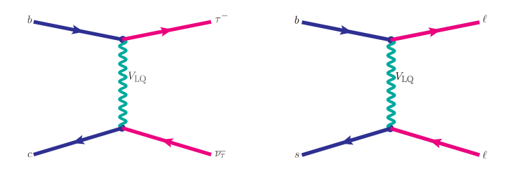
Figure 1: Feynman diagrams for $b\to c\tau^{-}\bar{\nu}_{\tau}$ (left panel) and $b\to s\ell^{+}\ell^{-}$ (right panel) processes mediated via VLQ, where $\ell=\mu,\tau$.

After having the idea about the NP contributions to the Wilson coefficients for both $b\to s\ell\ell$ and $b\to c\tau\bar{\nu}_{l}$, we now move forward to constrain these new parameters. For this purpose, we classify the new parameters into the following four scenarios:

• Scenario-I (S-I): Includes $C_{V_{1}}^{\rm LQ}$ for $b\to c\tau\bar{\nu}_{\tau}$ and $C_{9}^{\rm LQ}=-C_{10}^{\rm LQ}$ for $b\to s\ell\ell$ (contains only $LL$ couplings).

• Scenario-II (S-II): Includes $C_{9}^{\prime\rm LQ}=-C_{10}^{\prime\rm LQ}$ for $b\to s\ell\ell$ (involves only $RR$ couplings).

• Scenario-III (S-III): Includes $C_{S_{1}}^{\rm LQ}$ for $b\to c\tau\bar{\nu}_{\tau}$ and $-C_{P}^{\rm LQ}=C_{S}^{\rm LQ}$ for $b\to s\ell\ell$ (only $LR$ couplings present).

• Scenario-IV (S-IV): Includes $C_{P}^{\prime\rm LQ}=C_{S}^{\prime\rm LQ}$ for $b\to s\ell\ell$ (involves only $RL$ couplings).

These new couplings for various scenarios are constrained by performing a global fit (as discussed in Section V), to the relevant experimental observables as listed in the next section.

IV Observables used for Numerical fit

In our analysis, we consider the following most relevant flavor observables to constrain the new parameters.

IV.1 $\boldsymbol{b\to s\mu^{+}\mu^{-}}$

In the $b\to s\mu\mu$ sector, we include the following observables and their corresponding experimental data.

• $\boldsymbol{R_{K}}$ and $\boldsymbol{R_{K^{*}}}$: The lepton flavor universality violation ratios $R_{K}$ and $R_{K^{*}}$ are defined as

  $$R_{K}\ =\ \frac{{\rm BR}(B^{+}\to K^{+}\mu^{+}\mu^{-})}{{\rm BR}(B^{+}\to K^{+}e^{+}e^{-})}\,,\qquad R_{K^{*}}\ =\ \frac{{\rm BR}(B^{0}\to K^{*0}\mu^{+}\mu^{-})}{{\rm BR}(B^{0}\to K^{*0}e^{+}e^{-})}\,.$$ (8)

  In 2014, the measurement on the LFUV parameter $R_{K}$, in the low $q^{2}\in[1,6]~{}{\rm GeV}^{2}$ region by the LHCb experiment Aaij:2014ora :

  $$R_{K}^{\rm LHCb14}\ =\ \frac{{\rm BR}(B^{+}\to K^{+}\mu^{+}\mu^{-})}{{\rm BR}(B^{+}\to K^{+}e^{+}e^{-})}=0.745^{+0.090}_{-0.074}\pm 0.036\,,$$ (9)

  (where the first uncertainty is statistical and the second one is systematic) has attracted a lot of attention, as it amounted to a deviation of $2.6\sigma$ from its SM prediction  Bobeth:2007dw (see also Bordone:2016gaq )

  $$R_{K}^{\rm SM}\ =\ 1.0003\pm 0.0001\,.$$ (10)

  The updated LHCb measurement of $R_{K}$ in the $q^{2}\in[1.1,6]~{}{\rm GeV}^{2}$ region obtained by combining the data collected during three data-taking periods in which the c.o.m. energy of the collisions was 7, 8 and 13 TeV Aaij:2019wad

  $$R_{K}^{\rm LHCb19}\ =\ 0.846^{+0.060+0.016}_{-0.054-0.014}\,,$$ (11)

  also shows a discrepancy at the level of $2.5\sigma$.

  Analogously, the LHCb Collaboration has also measured the $R_{K^{*}}$ ratio in two bins of low- and high-$q^{2}$ regions Aaij:2017vbb :

  $$R_{K^{*}}^{\rm LHCb} \ =\ \begin{cases}0.660^{+0.110}_{-0.070}\pm 0.024\qquad q^{2}\in[0.045,1.1]~{}{\rm GeV}^{2}\,,\\ 0.685^{+0.113}_{-0.069}\pm 0.047\qquad q^{2}\in[1.1,6.0]~{}{\rm GeV}^{2}\,.\end{cases}$$ (12)

  which have respectively $2.2\sigma$ and $2.4\sigma$ deviations from their corresponding SM results Capdevila:2017bsm :

  $$R_{K^{*}}^{\rm SM}\ =\ \begin{cases}0.92\pm 0.02\qquad q^{2}\in[0.045,1.1]~{}{\rm GeV}^{2}\,,\\ 1.00\pm 0.01\qquad q^{2}\in[1.1,6.0]~{}{\rm GeV}^{2}\,.\end{cases}$$ (13)

  In addition to these LHCb results, Belle experiment has recently announced new measurements on $R_{K}$ Abdesselam:2019lab and $R_{K^{*}}$ Abdesselam:2019wac in several other bins:

  $$R_{K}^{\rm Belle}\ =\ \begin{cases}0.95^{+0.27}_{-0.24}\pm 0.06\qquad q^{2}\in[0.1,4.0]~{}{\rm GeV}^{2}\,,\\ 0.81^{+0.28}_{-0.23}\pm 0.05\qquad q^{2}\in[4.0,8.12]~{}{\rm GeV}^{2}\,,\\ 0.98^{+0.27}_{-0.23}\pm 0.06\qquad q^{2}\in[1.0,6.0]~{}{\rm GeV}^{2}\,,\\ 1.11^{+0.29}_{-0.26}\pm 0.07\qquad q^{2}>14.18~{}{\rm GeV}^{2}\,,\end{cases}$$ (14)

  $$R_{K^{*}}^{\rm Belle}\ =\ \begin{cases}0.52^{+0.36}_{-0.26}\pm 0.05\qquad q^{2}\in[0.045,1.1]~{}{\rm GeV}^{2}\,,\\ 0.96^{+0.45}_{-0.29}\pm 0.11\qquad q^{2}\in[1.1,6]~{}{\rm GeV}^{2}\,,\\ 0.90^{+0.27}_{-0.21}\pm 0.10\qquad q^{2}\in[0.1,8.0]~{}{\rm GeV}^{2}\,,\\ 1.18^{+0.52}_{-0.32}\pm 0.10\qquad q^{2}\in[15,19]~{}{\rm GeV}^{2}\,.\end{cases}$$ (15)

  One can notice that the Belle results have comparatively larger uncertainties than the LHCb measurements on $R_{K^{*}}$; therefore, we do not include the Belle results for $R_{K^{(*)}}$ in our fit for constraining the new parameters.

• $\boldsymbol{B_{s}\to\mu^{+}\mu^{-}}$: The current experimental value of the branching ratio of $B_{s}\to\mu^{+}\mu^{-}$ process is  Tanabashi:2018oca :

  $${\rm BR}(B_{s}^{0}\to\mu^{+}\mu^{-})\ =\ \left(3.0\pm 0.4\right)\times 10^{-9}\,,$$ (16)

  which is compatible with the SM prediction Bobeth:2013uxa

  $${\rm BR}(B_{s}^{0}\to\mu^{+}\mu^{-})^{\rm SM}\ =\ \left(3.65\pm 0.23\right)\times 10^{-9}\,,$$ (17)

  at $1.6\,\sigma$ confidence level (CL).

• Semileptonic $\boldsymbol{B_{(s)}}$ decays: We use the differential branching ratio measurements of $B^{+}\to K^{+(*)}\mu^{+}\mu^{-}$ Aaij:2014pli , $B^{0}\to K^{0(*)}\mu^{+}\mu^{-}$ Aaij:2014pli ; Aaij:2016flj and $B_{s}\to\phi\mu^{+}\mu^{-}$ Aaij:2015esa in different $q^{2}$ bins from LHCb, as listed in Table 3 . We have considered the forward-backward asymmetry $(A_{FB})$, longitudinal polarization asymmetry $(F_{L})$, form-factor independent observables ($P_{1,2,3},P_{4,5,6,8}^{\prime})$, CP-averaged angular coefficients $(S_{3,4,5,7,8,9})$ and CP asymmetries $(A_{3,4,5,6,7,8,9}$).

IV.2 $\boldsymbol{b\to c\tau\bar{\nu}_{\tau}}$

In this sector, we consider the following observables:

• $\boldsymbol{R_{D}}$ and $\boldsymbol{R_{D^{*}}}$: The lepton non-universality ratios $R_{D}$ and $R_{D^{*}}$ are defined as

  $$R_{D^{(*)}}\ =\ \frac{{\rm BR}(B\to D^{(*)}\tau\bar{\nu}_{\tau})}{{\rm BR}(B\to D^{(*)}\ell\bar{\nu}_{\ell})}\,,$$ (18)

  with $\ell=e,\mu$. These observables have been measured by the Belle Huschle:2015rga ; Hirose:2016wfn ; Abdesselam:2016cgx , BaBar Lees:2012xj ; Lees:2013uzd , and LHCb Aaij:2015yra ; Aaij:2017uff has measured only the $R_{D^{*}}$ parameter. Combining all these measurements, the averaged measured values of these ratios Amhis:2019ckw :

  $$R_{D}^{\rm Exp} \ =\ 0.34\pm 0.027\pm 0.013\,,$$ (19)

  $$R_{D^{*}}^{\rm Exp} \ =\ 0.295\pm 0.011\pm 0.008\,,$$ (20)

  induce a tension at the level of $3.08\sigma$ with the corresponding SM predictions Fajfer:2012vx ; Fajfer:2012jt ; Lattice:2015rga ; Na:2015kha ; Bigi:2017jbd ; Bernlochner:2017jka ; Jaiswal:2017rve ; Bernlochner:2020tfi ; Jaiswal:2020wer

  $$R_{D}^{\rm SM} \ =\ 0.299\pm 0.003\,,$$ (21)

  $$R_{D^{*}}^{\rm SM} \ =\ 0.258\pm 0.005\,.$$ (22)

• $\boldsymbol{R_{J/\psi}}$: Discrepancy of $1.7\sigma$ has also been observed between the experimental measurement of Aaij:2017tyk

  $$R_{J/\psi}^{\rm Exp}\ =\ \frac{{\rm BR}(B\to J/\psi\tau\bar{\nu}_{\tau})}{{\rm BR}(B\to J/\psi\ell\bar{\nu}_{\ell})}\ =\ 0.71\pm 0.17\pm 0.184\,,$$ (23)

  and the corresponding SM prediction Ivanov:2005fd ; Wen-Fei:2013uea ; Dutta:2017xmj ; Murphy:2018sqg ; Issadykov:2018myx ; Watanabe:2017mip ; Cohen:2018dgz ; Berns:2018vpl

  $$R_{J/\psi}^{\rm SM}\ =\ 0.289\pm 0.01\,.$$ (24)

• $\boldsymbol{B_{c}^{+}\to\tau^{+}\nu_{\tau}}$: This channel has not been measured yet, but indirect constraints on ${\rm BR}(B_{c}^{+}\to\tau^{+}\nu_{\tau})\lesssim 30\%$ have been imposed using the lifetime of $B_{c}$ Alonso:2016oyd (see also Refs. Li:2016vvp ; Celis:2016azn ). A stronger constraint of ${\rm BR}(B_{c}^{+}\to\tau^{+}\nu_{\tau})\lesssim 10\%$ was obtained from LEP data at the $Z$ peak Akeroyd:2017mhr . However, it assumes that the $B_{c}$ hadronization fraction measured in proton-proton collisions can be simply translated to $e^{+}e^{-}$ collisions and it uses this method to predict the number of $B_{c}$ mesons produced at LEP. However, $B_{c}$ production has not been observed at LEP, so there is a large uncertainty in this number, which was not considered in Ref. Akeroyd:2017mhr . Therefore, we will use the more conservative bound of $30\%$ on the $B_{c}^{+}\to\tau^{+}\nu_{\tau}$ branching ratio.

IV.3 $\boldsymbol{b\to s\tau^{+}\tau^{-}}$

In this sector, we consider the following two observables: ${\rm BR}(B_{s}\to\tau^{+}\tau^{-})<6.8\times 10^{-3}$ Aaij:2017xqt and ${\rm BR}(B^{+}\to K^{+}\tau^{+}\tau^{-})<2.2\times 10^{-3}$ TheBaBar:2016xwe .

IV.4 Comments

To estimate the SM values of the above-discussed observables, we use all the particles masses and lifetime of $B_{q}$ mesons from PDG Tanabashi:2018oca . The SM results of $B_{s}\to\mu^{+}\mu^{-}(\tau^{+}\tau^{-})$ processes are taken from Ref. Bobeth:2013uxa . The $B\to K$ form factors evaluated in the light cone sum rule (LCSR) approach Ball:2004ye are considered to estimate $B\to K\ell\ell$ processes in the SM. For $B_{(s)}\to K^{*}(\phi)\ell\ell$ decay modes, we use the form factors from Refs. Ball:2004rg ; Beneke:2004dp . The decay constant of $B_{c}$ meson is considered as $f_{B_{c}}=489$ MeV Chiu:2007km to compute branching ratio of $B_{c}\to\tau\nu_{\tau}$.

Since the singlet $({\bf 3,1},2/3)$ VLQ does not provide additional contributions to $b\to s\nu_{\ell}\bar{\nu}_{\ell}$ type decay modes at tree level due to charge conservation violation, the branching ratio of $B\to K^{(*)}\nu_{\ell}\bar{\nu}_{\ell}$ remains SM-like. Though the charge current $D$ meson decays mediated by $c\to s\ell\nu_{\ell}$ transitions such as $D_{s}^{+}\to\ell^{+}\nu_{\ell},\ D^{+}\to K^{0}\ell^{+}\nu_{\ell},\ D^{0}\to K^{(*)-}\ell^{+}\nu_{\ell}$ can also play a pivotal role in constraining VLQ couplings, however, they provide very weak bounds on these couplings. Thus, we do not consider these decay modes in our analysis. We further assume that the NP couplings associated with first-generation down-type quark and leptons are negligible. However, the coupling to up-type first generation quark can be non-vanishing via CKM matrix. Since we are mainly interested in the new couplings associated with second and third generation fermions, we do not consider the constraints coming from leptonic/semileptonic $K(D)$ meson decay modes and the $K^{0}-\overline{K}^{0}\ (D^{0}-\overline{D}^{0})$ mixing. We also do not consider the decays like $B_{u}\to\tau\nu_{\tau}$ which require new couplings to the first-generation fermions to have the $b\to u\tau\nu_{\tau}$ transition, which can be chosen to be small without affecting the $b\to c\tau\nu_{\tau}$ transitions, we are interested in.

The VLQ also contributes to loop-level flavor-changing processes, such as the $B_{s}-\overline{B}_{s}$ mixing, radiative $b\to s\gamma$ and $b\to s\nu\bar{\nu}$ decays, as well as $Z\to l_{i}\bar{l}_{j}$ decays. However, the simple VLQ model considered here is, by itself, non-renormalizable, which undermines the predictivity of these loop-level processes, unless some UV-complete framework generating the VLQ mass is explicitly specified; see e.g. Refs. Assad:2017iib ; DiLuzio:2017vat ; Bordone:2017bld ; Calibbi:2017qbu ; Blanke:2018sro ; Barbieri:2017tuq ; Greljo:2018tuh . Therefore, in the numerical analysis discussed below, we have considered only those processes which occur at tree-level through the exchange of a VLQ to derive constraints on our simplified model parameter space. However, we will consider a few loop-level processes for tau LFV prediction (see Section VI.7) and neutrino mass generation (see Section VII), which should be used with caution due to this caveat.

V Numerical Fits to model parameters

In this section, we consider the NP contributions to both $b\to s\ell\ell$ and $b\to c\tau\bar{\nu}_{\tau}$ processes, and fit the NP parameters by confronting the SM predictions with the observed data. The expression for $\chi^{2}$ used in our analysis is given by

$$\chi^{2}(C_{i}^{\rm LQ})\ =\ \sum_{i}\frac{\left[\mathcal{O}_{i}^{\rm th}(C_{i}^{\rm LQ})-\mathcal{O}_{i}^{\rm exp}\right]^{2}}{(\Delta\mathcal{O}_{i}^{\rm exp})^{2}+(\Delta\mathcal{O}_{i}^{\rm th})^{2}},$$ (25)

where $\mathcal{O}_{i}^{\rm th}(C_{i}^{\rm LQ})$ are the theoretical predictions for the observables used in this fit, which depend on the new Wilson coefficients $(C_{i}^{\rm LQ})$ arising due to the VLQ exchange and $\Delta\mathcal{O}_{i}^{\rm th}$ contains the $1\sigma$ error from theory. Here $\mathcal{O}_{i}^{\rm exp}$ and $\Delta\mathcal{O}_{i}^{\rm exp}$ respectively represent the corresponding experimental central value and $1\sigma$ uncertainty for the observables. All feasible new parameters of the VLQ model with $V_{\rm LQ}({\bf 3},{\bf 1},2/3)$, which provide a good fit to both $b\to s\ell\ell$ and $b\to c\tau\bar{\nu}_{\tau}$ data are discussed in Refs. Buttazzo:2017ixm ; Bhattacharya:2016mcc ; Kumar:2018kmr . For concreteness, we fix the VLQ mass at $M_{V_{\rm LQ}}=1.2$ TeV in the following analysis, which is consistent with the current LHC constraints Sirunyan:2018kzh .

We consider various possible sets of data to fit different scenarios of new Wilson coefficients. These different cases are further classified as follows.

• : Includes measurement on $B$ decay modes with only third generation leptons in the final state

  • C-Ia: Only $b\to c\tau\bar{\nu}_{\tau}$.

  • C-Ib: Both $b\to c\tau\bar{\nu}_{\tau}$ and $b\to s\tau^{+}\tau^{-}$.

• : Includes measurement on $B$ decay modes with only second generation leptons in the final state, i.e., $b\to s\mu^{+}\mu^{-}$.

• : Includes measurement on $B$ decay modes, which decay either to third generation or second generation leptons, i.e., $b\to c\tau\bar{\nu}_{\tau}$, $b\to s\tau^{+}\tau^{-}$ and $b\to s\mu^{+}\mu^{-}$.

In Fig. 2 , we show the constraints on new leptoquark couplings by using different data sets of above discussed observables for Scenario-I (see Section III), which includes only $LL$ type operators, i.e. $C_{V_{1}}^{\rm LQ}$ contribution from $b\to c\tau\bar{\nu}_{\tau}$ and $C_{9,10}^{\rm LQ}$ from $b\to s\ell^{+}\ell^{-}$. Here, the constraint plots for the new couplings for C-Ia (left), C-Ib (middle) and C-II (right) cases are presented in the top panel. The bottom panel of Fig. 2 represents the constraint plots for C-III in the $\lambda_{33}^{L}-\lambda_{23}^{L}$ (left) and $\lambda_{32}^{L}-\lambda_{22}^{L}$ (right) panels. In each plot of Fig. 2 , different colors represent the $1\sigma$, $2\sigma$, and $3\sigma$ contours and the black dot stands for the best-fit value. The corresponding best-fit values obtained for various cases are presented in Table 1 . In this Table, we have also provided the $\chi^{2}_{\rm min,VLQ+SM}/{\rm d.o.f}$ as well as the pull$=\sqrt{\chi_{\rm SM}^{2}-\chi^{2}_{\rm best-fit}}$ values. For C-Ia case, we have $4$ observables with two parameters for fit, thus the number of degrees of freedom (d.o.f.) is 2. Here we find $\chi^{2}_{\rm min}/{\rm d.o.f}=2.3/2=1.15$, which implies the fit is acceptable. The $\chi^{2}_{\rm min}/{\rm d.o.f}$ for C-Ib case is found to be $0.58$ i.e., the singlet VLQ can explain both $b\to c\tau\bar{\nu}_{\tau}$ and $b\to s\tau^{+}\tau^{-}$ data simultaneously. We find $\chi_{\rm min,VLQ+SM}^{2}/{\rm d.o.f}<1$ for both C-II and C-III cases, which implies the VLQ can accommodate $b\to s\tau\tau(\mu\mu)$ anomalies as well as the issues in both $b\to s\tau\tau(\mu\mu)$ and $b\to c\tau\bar{\nu}_{\tau}$ very well. This analysis implies that the presence of only $LL$ type VLQ couplings can illustrate the $B$ anomalies associated with both $b\to c\tau\bar{\nu}_{\tau}$ and $b\to s\ell\ell$ kind of processes on equal footing.

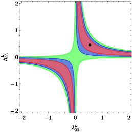
(a)  C-Ia case of Scenario-I

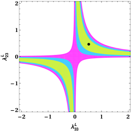
(b)  C-Ib case of Scenario-I

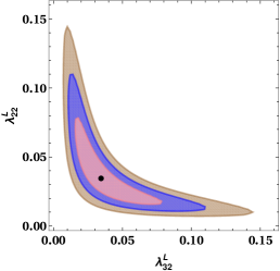
(c)  C-II case of Scenario-I

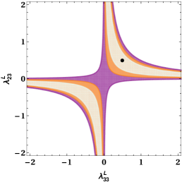
(d)  C-III case of Scenario-I in $\lambda_{33}^{L}-\lambda_{23}^{L}$ plane

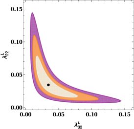
(e)  C-III case of Scenario-I in $\lambda_{32}^{L}-\lambda_{22}^{L}$ plane

Figure 2: Constraints on new VLQ couplings which include only $LL$ type operators (Scenario-I) for different sets of observables. Different colors represent the $1\sigma$, $2\sigma$, and $3\sigma$ contours and the black dot stands for the best-fit value.

In Scenario-II with the new leptoquark couplings of $RR$ operator type, the constraint on the new couplings associated with right-handed quark and lepton singlets is depicted in Fig. 3 . Since the VLQ has no $\lambda_{ij}^{R}$ type coupling contribution to $b\to c\tau\bar{\nu}_{\tau}$, so we fit the new $\lambda_{ij}^{R}$ parameters from only $b\to s\mu\mu$ data (C-II case of our analysis). In Table 1 , the best-fit values and the $\chi^{2}_{\rm min}/{\rm d.o.f}$ for this scenario are shown. Here the value of $\chi^{2}_{\rm min}/{\rm d.o.f}=1.04$ is very close to one, implying that the fit is acceptable.

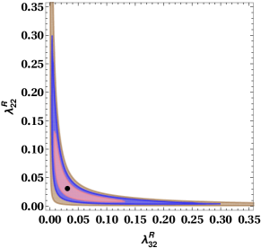
Figure 3: Constraints on new VLQ couplings of $RR$-type with quark and lepton singlets (Scenario-II). Here only C-II case is relevant. Different colors represent the $1\sigma$, $2\sigma$, and $3\sigma$ contours and the black dot stands for the best-fit value.

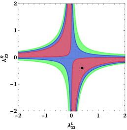
(a)  C-Ia case of Scenario-III

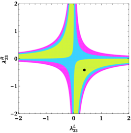
(b)  C-Ib case of Scenario-III

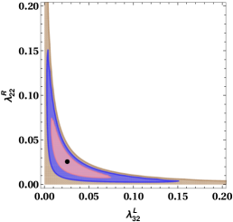
(c)  C-II case of Scenario-III

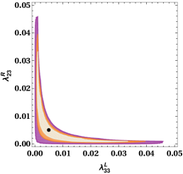
(d)  C-III case of Scenario-III in $\lambda_{33}^{L}-\lambda_{23}^{R}$ plane

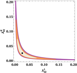
(e)  C-III case of Scenario-III in $\lambda_{32}^{L}-\lambda_{22}^{R}$ plane

Figure 4: Constraints on new VLQ couplings which include only $LR$-type operators (Scenario-III) for different data sets of observables. Different colors represent the $1\sigma$, $2\sigma$, and $3\sigma$ contours and the black dot stands for the best-fit value.

Fig. 4 depicts the constraints on $LR$ -type couplings (Scenario III) associated with unprimed pseudo(scalar) operators for different sets of data. The corresponding best-fit values and $\chi^{2}_{\rm min}/{\rm d.o.f}$ for different cases are given in Table 1 . The $\chi^{2}_{\rm min}/{\rm d.o.f}$ is found to be $4.235~{}(2.11)$ for C-Ia (C-Ib), which means the fit is rather poor. The $\chi^{2}_{\rm min}/{\rm d.o.f}$ for both C-II and C-III cases are slightly greater than $1$. Thus, the presence of only pseudo(scalar) type couplings arising due to the exchange of VLQ is not good enough to explain the anomalies in both $b\to c\tau\bar{\nu}_{\tau}$ and $b\to s\ell\ell$ processes.

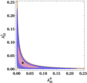
Figure 5: Constraints on new VLQ couplings of $RL$-type with quark and lepton singlets (Scenario-IV). Different colors represent the $1\sigma$, $2\sigma$, and $3\sigma$ contours and the black dot stands for the best-fit value.

Fig. 5 represents constraints on new $RL$-type couplings (Scenario-IV) obtained from only $b\to s\mu\mu$ observables (C-II case). The obtained best-fit value and $\chi^{2}_{\rm min}/{\rm d.o.f}$ are give in Table 1 . We notice that $\chi^{2}_{\rm min}/{\rm d.o.f}$ is slightly larger than one. Though the fit is not as good as Scenario-I, but still it is acceptable.

As can be seen from Table 1, the case C-III in Scenario-I with $C_{9,{\rm NP}}^{\mu\mu}=-C_{10,{\rm NP}}^{\mu\mu}$ provides the best-fit to all the observables in $b\to s\mu^{+}\mu^{-}$ and $R_{K^{(*)}}$. This is in agreement with the recent global-fit results Aebischer:2019mlg which include the latest LHCb measurements of $R_{K}$. If the fit is done separately, i.e., one for all the data involving $b\to s\mu^{+}\mu^{-}$ and the other for $R_{K^{(*)}}$ observables, there is a slight tension between the NP Wilson coefficients required to explain the $b\to s\mu^{+}\mu^{-}$ and the $R_{K^{(*)}}$ data, which can be addressed by considering NP contribution to $b\to se^{+}e^{-}$ process as well Datta:2019zca . However, in this case, one has to take into account the additional constraint from the LFV process $\mu\to e\gamma$. Since in our framework, the LQ is not coupled to the first generation of fermions, we do not encounter any NP contribution to $b\to se^{+}e^{-}$ process nor to the LFV process $\mu\to e\gamma$.

Scenarios	Cases	Couplings	Best-fit Values	$\chi^{2}_{\rm min}/{\rm d.o.f}$	Pull
	C-Ia	$(\lambda^{L}_{33},~{}{\lambda^{L}_{23}})$	$(0.451,0.631)$	$1.15$	$2.982$
S-I	C-Ib	$(\lambda^{L}_{33},~{}{\lambda^{L}_{23}})$	$(0.475,0.595)$	$0.58$	$2.979$
	C-II	$(\lambda^{L}_{32},~{}{\lambda^{L}_{22}})$	$(0.035,0.035)$	$0.931$	$5.78$
	C-III	$(\lambda^{L}_{33},~{}{\lambda^{L}_{23}},\lambda^{L}_{32},~{}{\lambda^{L}_{22}})$	$(0.56,0.51,0.0351,0.0351)$	$0.926$	$6.1$
S-II	C-II	$(\lambda^{R}_{32},~{}{\lambda^{R}_{22}})$	$(0.0315,0.0315)$	$1.04$	$3.499$
	C-Ia	$(\lambda^{L}_{33},~{}{\lambda^{R}_{23}})$	$(0.44,-0.44)$	$4.235$	$1.65$
S-III	C-Ib	$(\lambda^{L}_{33},~{}{\lambda^{R}_{23}})$	$(0.42,-0.462)$	$2.11$	$1.66$
	C-II	$(\lambda^{L}_{32},~{}{\lambda^{R}_{22}})$	$(0.0254,0.0254)$	$1.05$	$3.049$
	C-III	$(\lambda^{L}_{33},~{}{\lambda^{R}_{23}},\lambda^{L}_{32},~{}{\lambda^{R}_{22}})$	$(0.005,0.005,0.0258,0.0258)$	$1.043$	$4.28$
S-IV	C-II	$(\lambda^{R}_{32},~{}{\lambda^{L}_{22}})$	$(0.0233,0.0233)$	$1.063$	$2.67$

Table 1: Best-fit values of new VLQ couplings, $\chi^{2}_{\rm min}/{\rm d.o.f}$ and pull values for different cases of all scenarios (S-I, S-II, S-III, S-IV).

VI Implications on Lepton flavor violating $B$ and tau decay modes

This section will be dedicated to the study of LFV two/three body decay modes of $B$ meson and $\tau$ lepton in the presence of the VLQ, $V_{\rm LQ}({\bf 3,1},2/3)$. The rare leptonic/semileptonic LFV $B$ channels involving $b\to sl_{i}^{-}l_{j}^{+}$ quark-level transition, occur at tree level due to the exchange of VLQ. The left panel of Fig. 6 depicts the Feynman diagram of $b\to s\tau\mu$ LFV decay modes at tree level.

The total effective Hamiltonian for $b\to sl_{i}^{-}l_{j}^{+}$ processes in the VLQ model can be written as

$$\mathcal{H}_{\rm eff}\left(b\to sl_{i}^{-}l_{j}^{+}\right)\ =\ \mathcal{H}_{\rm eff}^{\rm VA}+\mathcal{H}_{\rm eff}^{\rm SP},$$ (26)

where the vector-axial vector (VA) and scalar-pseudoscalar (SP) parts are given by

$$\mathcal{H}_{\rm eff}^{\rm VA} \ =\ -\frac{G_{F}\alpha_{\rm em}}{\sqrt{2}\pi}V_{tb}V_{ts}^{*}\Big{[}C_{9}^{\rm LQ}\left(\bar{s}\gamma^{\mu}P_{L}b\right)\left(\bar{l}_{i}\gamma_{\mu}l_{j}\right)+C_{10}^{\rm LQ}\left(\bar{s}\gamma^{\mu}P_{L}b\right)\left(\bar{l}_{i}\gamma_{\mu}\gamma_{5}l_{j}\right)$$

$$+ C_{9}^{\prime\rm LQ}\left(\bar{s}\gamma^{\mu}P_{R}b\right)\left(\bar{l}_{i}\gamma_{\mu}l_{j}\right)+C_{10}^{\prime\rm LQ}\left(\bar{s}\gamma^{\mu}P_{R}b\right)\left(\bar{l}_{i}\gamma_{\mu}\gamma_{5}l_{j}\right)\Big{]},~{}~{}~{}$$

$$\mathcal{H}_{\rm eff}^{\rm SP} \ =\ -\frac{G_{F}\alpha_{\rm em}}{\sqrt{2}\pi}V_{tb}V_{ts}^{*}\Big{[}C_{S}^{\rm LQ}\left(\bar{s}P_{R}b\right)\left(\bar{l}_{i}l_{j}\right)+C_{P}^{\rm LQ}\left(\bar{s}P_{R}b\right)\left(\bar{l}_{i}\gamma_{5}l_{j}\right)$$

$$+ C_{S}^{\prime\rm LQ}\left(\bar{s}P_{L}b\right)\left(\bar{l}_{i}l_{j}\right)+C_{P}^{\prime\rm LQ}\left(\bar{s}P_{L}b\right)\left(\bar{l}_{i}\gamma_{5}l_{j}\right)\Big{]}.$$ (27)

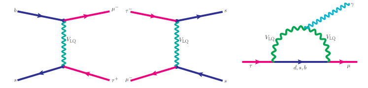
Figure 6: Feynman diagrams for lepton-flavor-violating $b\to s\tau^{+}\mu^{-}$ (left panel), $\tau\to\mu\phi~{}(\eta^{(\prime)})$ (middle panel) and $\tau\to\mu\gamma$ (bottom panel) processes mediated via the VLQ.

This leads to the following LFV processes:

VI.1 $\boldsymbol{B_{s}\to l_{i}^{-}l_{j}^{+}}$

The branching ratio of the LFV $B_{s}\to l_{i}^{-}l_{j}^{+}$ decay process in the presence of VLQ is given as  Becirevic:2016zri

$${\rm BR}(B_{s}\to l_{i}^{-}l_{j}^{+})\ =\ \tau_{B_{s}}\frac{\alpha_{\mathrm{em}}^{2}G_{F}^{2}}{64\pi^{3}M_{B_{s}}^{3}}f_{B_{s}}^{3}|V_{tb}V_{ts}^{*}|^{2}\lambda^{1/2}(M_{B_{s}},m_{i},m_{j})$$

$$\times\Bigg{[}[M_{B_{s}}^{2}-(m_{i}+m_{j})^{2}]\Bigg{|}(C_{9}^{\rm LQ}-C_{9}^{\prime\rm LQ})(m_{i}-m_{j})+(C_{S}^{\rm LQ}-C_{S}^{\prime\rm LQ})\frac{M_{B_{s}}^{2}}{m_{b}+m_{s}}\Bigg{|}^{2}$$

$$+[M_{B_{s}}^{2}-(m_{i}-m_{j})^{2}]\Bigg{|}(C_{10}^{\rm LQ}-C_{10}^{\prime\rm LQ})(m_{i}+m_{j})+(C_{P}^{\rm LQ}-C_{P}^{\prime\rm LQ})\frac{M_{B_{s}}^{2}}{m_{b}+m_{s}}\Bigg{|}^{2}\Bigg{]},$$ (28)

where $f_{B_{s}}$ is the $B_{s}$ decay constant and

$$\lambda(a,b,c)\ =\ a^{4}+b^{4}+c^{4}-2\left(a^{2}b^{2}+b^{2}c^{2}+a^{2}c^{2}\right)$$ (29)

is the so-called triangle function.

VI.2 $\boldsymbol{B\to Kl_{i}^{-}l_{j}^{+}}$

The differential branching ratio of $\overline{B}\to\overline{K}l_{i}^{-}l_{j}^{+}$ process is given as Duraisamy:2016gsd

$$\frac{{\rm d}{\rm BR}}{{\rm d}q^{2}}(\overline{B}\to\overline{K}l_{i}^{-}l_{j}^{+}) \ =\ \tau_{B}\frac{G_{F}^{2}\alpha^{2}_{\rm em}}{2^{12}\pi^{5}M_{B}^{3}}\beta_{ij}\sqrt{\lambda(M_{B}^{2},M_{K}^{2},q^{2})}|V_{tb}V_{ts}^{*}|^{2}\sum_{i=1}^{6}J_{i},$$ (30)

$${\rm where}\quad\beta_{ij} \ =\ \sqrt{\left(1-\frac{(m_{i}+m_{j})^{2}}{q^{2}}\right)\left(1-\frac{(m_{i}-m_{j})^{2}}{q^{2}}\right)}\,.$$ (31)

The coefficients $J_{i}$ in Eq. (30) are given in Appendix B.

VI.3 $\boldsymbol{B\to K^{*}l_{i}^{-}l_{j}^{+}}$ and $\boldsymbol{B_{s}\to\phi l_{i}^{-}l_{j}^{+}}$

Including the VLQ contribution, the differential branching ratio of $\overline{B}\to\overline{K}^{*}l_{i}^{-}l_{j}^{+}$ decay process is given by Becirevic:2016zri

$$\frac{\mathrm{d}{\rm BR}}{\mathrm{d}q^{2}}(\overline{B}\to\overline{K}^{*}l_{i}^{-}l_{j}^{+})\ =\ \dfrac{1}{4}\left[3I_{1}^{c}(q^{2})+6I_{1}^{s}(q^{2})-I_{2}^{c}(q^{2})-2I_{2}^{s}(q^{2})\right],$$ (32)

where the expressions for the angular coefficients $I_{i}(q^{2})$ are provided in Appendix C . The same expression can be applied to $B_{s}\to\phi l_{i}l_{j}$ process with appropriate changes in the particles masses and the lifetime of $B_{s}$ meson.

Assuming that there is no NP contribution to the first-generation fermions, here we compute the branching fractions for the LFV decay modes of $B$ meson to second and third generation leptons only. One can also notice that the leptoquark couplings required to investigate the above-defined LFV decay modes are present in the C-III scenario of our analysis, which includes both $b\to c\tau\bar{\nu}_{\tau}$ and $b\to s\tau\tau(\mu\mu)$ types of processes. For the numerical estimates, all the required $B$ meson masses and lifetimes are taken from PDG Tanabashi:2018oca  . Using $f_{B_{s}}=(225.6\pm 1.1\pm 5.4)$ MeV Charles:2015gya and the best-fit values of the constrained new parameters of S-I and S-III from Table 1 , we present our predictions on various LFV branching ratios of $B$ mesons in Table 2 . From the table, one can notice that, the branching ratios of the LFV $B$ decays are quite significant in S-I scenario and are within the reach of Belle or LHCb experiments. However, the experimental limits on most of these decay modes are not yet available. The only LFV channels that have been looked for are $B^{+}\to K^{+}\mu^{-}\tau^{+}(\mu^{+}\tau^{-})$ Lees:2012zz and $B_{s}\to\tau^{\pm}\mu^{\mp}$ Aaij:2019okb for which we find our predictions for the branching ratios are well below the current 90% CL experimental upper limits. Our predictions on branching ratio of $B_{s}\to\tau^{\pm}\mu^{\mp}$ process,

$${\rm BR}(B_{s}\to\tau^{\pm}\mu^{\mp})\ = \ {\rm BR}(B_{s}\to\tau^{+}\mu^{-})+{\rm BR}(B_{s}\to\tau^{-}\mu^{+})$$ (35)

$$\ =\ \left\{\begin{array}[]{ll}6.0\times 10^{-7}&{\rm for~{}S-I}\,,\\ 1.3\times 10^{-9}&{\rm for~{}S-III}\,,\end{array}\right.$$

which is much lower than the current experimental limit at 90% C.L. Aaij:2019okb :

$${\rm BR}(B_{s}\to\tau^{\pm}\mu^{\mp})|^{\rm Exp}\ <\ 3.4\times 10^{-5}\,.$$ (36)

Our estimated branching ratios of the LFV processes $B_{(s)}\to(K,K^{*},\phi)\mu^{-}\tau^{+}(\mu^{+}\tau^{-})$ even for Scenario-III are reasonable and within the reach of future $B$-physics experiments, such as LHCb upgrade Bediaga:2018lhg and Belle-II Kou:2018nap .

In Fig. 7 , we show the variation of differential branching ratios of $B^{+}\to K^{+}\mu^{-}\tau^{+}$ (top-left panel), $B^{+}\to K^{*+}\mu^{-}\tau^{+}$ (top-right panel) and $B_{s}\to\phi\mu^{-}\tau^{+}$ (bottom panel) processes with respect to $q^{2}$ for C-III of Scenario-I in the presence of VLQ; cf. Eqs. (30), (32) .

Decay	Predicted values		Experimental Limit
modes	S-I	S-III	(90% CL)
$B_{s}\to\mu^{-}\tau^{+}$	$2.7\times 10^{-7}$	$6.7\times 10^{-10}$	$<3.4\times 10^{-5}$ Aaij:2019okb
$B^{+}\to K^{+}\mu^{-}\tau^{+}$	$1.3\times 10^{-6}$	$3.0\times 10^{-10}$	$<2.8\times 10^{-5}$ Lees:2012zz
$\overline{B}^{0}\to\overline{K}^{0}\mu^{-}\tau^{+}$	$1.2\times 10^{-6}$	$2.8\times 10^{-10}$	$\cdots$
$B^{+}\to K^{*+}\mu^{-}\tau^{+}$	$2.6\times 10^{-6}$	$1.11\times 10^{-10}$	$\cdots$
$\overline{B}^{0}\to\overline{K}^{*0}\mu^{-}\tau^{+}$	$2.4\times 10^{-6}$	$1.0\times 10^{-10}$	$\cdots$
$B_{s}\to\phi\mu^{-}\tau^{+}$	$3.1\times 10^{-6}$	$1.4\times 10^{-10}$	$\cdots$
$B_{s}\to\mu^{+}\tau^{-}$	$3.3\times 10^{-7}$	$6.7\times 10^{-10}$	$<3.4\times 10^{-5}$ Aaij:2019okb
$B^{+}\to K^{+}\mu^{+}\tau^{-}$	$1.6\times 10^{-6}$	$3.0\times 10^{-10}$	$<4.5\times 10^{-5}$ Lees:2012zz
$\overline{B}^{0}\to\overline{K}^{0}\mu^{+}\tau^{-}$	$1.5\times 10^{-6}$	$2.8\times 10^{-10}$	$\cdots$
$B^{+}\to K^{*+}\mu^{+}\tau^{-}$	$3.1\times 10^{-6}$	$1.1\times 10^{-10}$	$\cdots$
$\overline{B}^{0}\to\overline{K}^{*0}\mu^{+}\tau^{-}$	$2.9\times 10^{-6}$	$1.0\times 10^{-10}$	$\cdots$
$B_{s}\to\phi\mu^{+}\tau^{-}$	$3.8\times 10^{-6}$	$1.4\times 10^{-10}$	$\cdots$
$\Upsilon(1S)\to\mu^{-}\tau^{+}$	$1.8\times 10^{-11}$	$7.7\times 10^{-16}$	$\cdots$
$\Upsilon(2S)\to\mu^{-}\tau^{+}$	$1.8\times 10^{-11}$	$7.9\times 10^{-16}$	$\cdots$
$\Upsilon(3S)\to\mu^{-}\tau^{+}$	$2.4\times 10^{-11}$	$1.0\times 10^{-15}$	$\cdots$
$\Upsilon(1S)\to\mu^{+}\tau^{-}$	$1.8\times 10^{-11}$	$7.7\times 10^{-16}$	$\cdots$
$\Upsilon(2S)\to\mu^{+}\tau^{-}$	$1.8\times 10^{-11}$	$7.9\times 10^{-16}$	$\cdots$
$\Upsilon(3S)\to\mu^{+}\tau^{-}$	$2.4\times 10^{-11}$	$1.0\times 10^{-15}$	$\cdots$
$\tau^{-}\to\mu^{-}\phi$	$2.0\times 10^{-8}$	$1.0\times 10^{-12}$	$<8.4\times 10^{-8}$ Miyazaki:2011xe
$\tau^{-}\to\mu^{-}\eta$	$2.1\times 10^{-8}$	$1.1\times 10^{-12}$	$<6.5\times 10^{-8}$ Tanabashi:2018oca
$\tau^{-}\to\mu^{-}\eta^{\prime}$	$6.8\times 10^{-10}$	$3.5\times 10^{-14}$	$<1.3\times 10^{-7}$ Tanabashi:2018oca
$\tau^{-}\to\mu^{-}\gamma$	$4.8\times 10^{-9}$	$\cdots$	$<4.4\times 10^{-8}$ Aubert:2009ag

Table 2: Predicted branching ratios of lepton flavor violating decay modes of $B$ meson and $\tau$ lepton in the VLQ model for C-III case in Scenario-I and Scenario-III.

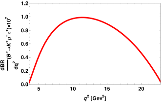
(a)  $B^{+}\to K^{+}\mu^{-}\tau^{+}$

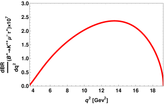
(b)  $B^{+}\to K^{*+}\mu^{-}\tau^{+}$

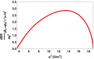
(c)  $B_{s}\to\phi\mu^{-}\tau^{+}$

Figure 7: The $q^{2}$ variation of branching ratios of $B^{+}\to K^{+}\mu^{-}\tau^{+}$ (top-left panel), $B^{+}\to K^{*+}\mu^{-}\tau^{+}$ (top-right panel) and $B_{s}\to\phi\mu^{-}\tau^{+}$ (bottom panel) processes in the presence of VLQ.

In the following two subsections, we study the LFV decay modes of $\Upsilon(nS)$ and the $\tau$ lepton.

VI.4 ${\boldsymbol{\Upsilon(nS)\to\mu\tau}}$

The Feynman diagram for LFV $\Upsilon(nS)\to\mu\tau$ channel can be obtained from the diagram for $b\to s\mu\tau$ decay mode (left panel of Fig. 6) by replacing $s\to b$. The branching ratio of $\Upsilon(nS)\to\mu^{-}\tau^{+}$ decay mode is given by Bhattacharya:2016mcc

$${\rm BR}(\Upsilon(nS)\to\mu^{-}\tau^{+})\ = \ \frac{f_{\Upsilon(nS)}^{2}m_{\Upsilon(nS)}^{3}}{48\pi\Gamma_{\Upsilon(nS)}}\left(2-\frac{m_{\tau}^{2}}{m_{\Upsilon(nS)}^{2}}-\frac{m_{\tau}^{4}}{m_{\Upsilon(nS)}^{4}}\right)\left(1-\frac{m_{\tau}^{2}}{m_{\Upsilon(nS)}^{2}}\right)\left|\frac{\lambda^{L}_{32}\lambda^{L*}_{33}}{M_{V_{\rm LQ}}^{2}}\right|^{2}\,.$$ (37)

The branching ratio expresion for $\Upsilon(nS)\to\mu^{+}\tau^{-}$ process can be obtained from $\Upsilon(nS)\to\mu^{-}\tau^{+}$ by replacing the LQ coupling $\lambda^{L}_{32}\lambda^{L*}_{33}\to\lambda^{L}_{33}\lambda^{L*}_{32}$. For numerical calculation, we take all the particle mases and the width of $\Upsilon(nS),~{}n=1,2,3$ from PDG Tanabashi:2018oca  . The values of decay constants of $\Upsilon(nS)$ used in our analysis are $f_{\Upsilon(1S)}=(700\pm 16)$ MeV, $f_{\Upsilon(2S)}=(496\pm 21)$ MeV and $f_{\Upsilon(3S)}=(430\pm 21)$ MeV Bhattacharya:2016mcc  . The case C-III of both S-I and S-III scenarios include the LQ couplings required for $\Upsilon(nS)\to\mu^{+}\tau^{-}$ branching ratio computation, whose best-fit values are given in Table 1 . Now, using all the input parameters, the predicted branching ratios of $\Upsilon(nS)\to\mu^{-}\tau^{+}$ ($\Upsilon(nS)\to\mu^{+}\tau^{-}$) are provided in Table 2 . Using the branching ratio expression of $\Upsilon(nS)\to\mu^{\mp}\tau^{\pm}$ proceses as

$${\rm BR}(\Upsilon(nS)\to\mu^{\mp}\tau^{\pm})={\rm BR}(\Upsilon(nS)\to\mu^{-}\tau^{+})+{\rm BR}(\Upsilon(nS)\to\mu^{+}\tau^{-})\,,$$ (38)

our predictions in the presence of VLQ are given by

$${\rm BR}(\Upsilon(1S)\to\mu^{\mp}\tau^{\pm}) \ =\ \left\{\begin{array}[]{ll}3.6\times 10^{-11}&{\rm for~{}S-I}\,,\\ 1.5\times 10^{-15}&{\rm for~{}S-III}\,,\end{array}\right.$$ (41)

$${\rm BR}(\Upsilon(2S)\to\mu^{\mp}\tau^{\pm}) \ =\ \left\{\begin{array}[]{ll}3.6\times 10^{-11}&{\rm for~{}S-I}\,,\\ 1.6\times 10^{-15}&{\rm for~{}S-III}\,,\end{array}\right.$$ (44)

$${\rm BR}(\Upsilon(3S)\to\mu^{\mp}\tau^{\pm}) \ =\ \left\{\begin{array}[]{ll}4.8\times 10^{-11}&{\rm for~{}S-I}\,,\\ 2.1\times 10^{-15}&{\rm for~{}S-III}\,,\end{array}\right.$$ (47)

which are much lower than the current experimental upper limits Tanabashi:2018oca :

$${\rm BR}(\Upsilon(1S)\to\mu^{\mp}\tau^{\pm})|^{\rm Exp}\ <\ 6.0\times 10^{-6}~{}~{}~{}~{}95\%~{}{\rm CL}\,,$$

$${\rm BR}(\Upsilon(2S)\to\mu^{\mp}\tau^{\pm})|^{\rm Exp}\ <\ 3.3\times 10^{-6}~{}~{}~{}~{}90\%~{}{\rm CL}\,,$$

$${\rm BR}(\Upsilon(3S)\to\mu^{\mp}\tau^{\pm})|^{\rm Exp}\ <\ 3.1\times 10^{-6}~{}~{}~{}~{}90\%~{}{\rm CL}\,.$$ (48)

VI.5 ${\boldsymbol{\tau\to\mu\phi}}$

The Feynman diagram for $\tau\to\mu\phi$ LFV decay process is presented in the middle panel of Fig. 6 . The branching ratio of $\tau\to\mu\phi$ channel is given by Becirevic:2016oho

$${\rm BR}(\tau\to\mu\phi)\ = \ \frac{\tau_{\tau}f_{\phi}^{2}m_{\phi}^{4}}{128\pi m_{\tau}^{3}}\left|\frac{\lambda^{L}_{23}\lambda^{L*}_{22}+\lambda^{R}_{23}\lambda^{R*}_{22}}{M_{V_{\rm LQ}}^{2}}\right|^{2}$$ (49)

$$\times\lambda^{1/2}(m_{\phi}^{2},m_{\tau}^{2},m_{\mu}^{2})\left[-1+\frac{(m_{\mu}^{2}+m_{\tau}^{2})}{2m_{\phi}^{2}}+\frac{(m_{\mu}^{2}-m_{\tau}^{2})^{2}}{2m_{\phi}^{4}}\right],$$

where $f_{\phi}$ is the decay constant of $\phi$ meson. Using the values of various masses and lifetime of $\tau$ from PDG Tanabashi:2018oca , $f_{\phi}=(238\pm 3)$ MeV from Ref. Chakraborty:2017hry and best-fit values of required new parameters for C-III case of Scenario-I and Scenario-III from Table 1 , we estimate the branching fraction of $\tau\to\mu\phi$ as shown in Table 2 . We find that the $\tau^{-}\to\mu^{-}\phi$ branching ratio is substantially enhanced in S-I scenario; it is just below the current experimental upper limit Miyazaki:2011xe and within the reach of Belle-II experiment.

VI.6 ${\boldsymbol{\tau\to\mu\eta^{(\prime)}}}$

The branching ratio of $\tau\to\mu\eta^{(\prime)}$ process is given by Bhattacharya:2016mcc

$${\rm BR}(\tau\to\mu\eta^{(\prime)})\ = \ \frac{\tau_{\tau}f_{\eta^{(\prime)}}^{2}m_{\tau}^{3}}{128\pi}\left|\frac{\lambda^{L}_{23}\lambda^{L*}_{22}+\lambda^{R}_{23}\lambda^{R*}_{22}}{M_{V_{\rm LQ}}^{2}}\right|^{2}\left(1-\frac{m_{\eta^{(\prime)}}^{2}}{m_{\tau}^{2}}\right)\,.$$ (50)

Using $f_{\eta}\simeq-157.63$ MeV Bhattacharya:2016mcc , $f_{\eta^{\prime}}\simeq 31.76$ MeV Bhattacharya:2016mcc , alongwith other input parameters from Tanabashi:2018oca and the best-fit values of LQ couplings from Table 1 , the estimated values of branching ratios of $\tau\to\mu\eta^{(\prime)}$ are presented in Table 2 , which are found to be well below the current experimental upper limits.

VI.7 ${\boldsymbol{\tau\to\mu\gamma}}$

The right panel of Fig. 6 represents the one loop Feynman diagram for radiative $\tau\to\mu\gamma$ channel. The effective Hamiltonian for radiative $\tau^{-}\to\mu^{-}\gamma$ decay mode can be expressed as Lavoura:2003xp

$$\mathcal{H}_{\rm eff}\ =\ e\Bigg{(}C_{L}\bar{\mu}_{R}\sigma^{\mu\nu}F_{\mu\nu}\tau_{L}+C_{R}\bar{\mu}_{L}\sigma^{\mu\nu}F_{\mu\nu}\tau_{R}\Bigg{)}\,.$$ (51)

Here $\sigma^{\mu\nu}$ is the photon field strength tensor and the Wilson coefficients $C_{L(R)}$ generated due to VLQ exchange are given as

$$C_{L} \ =\ \frac{N_{c}}{16\pi^{2}M_{V_{\rm LQ}}^{2}}\Bigg{(}-\frac{1}{3}\Bigg{[}\lambda^{L}_{33}{\lambda^{L}_{32}}^{*}f_{2}(x_{b})+\lambda^{R}_{33}{\lambda^{R}_{32}}^{*}f_{1}(x_{b})+\lambda^{L}_{33}{\lambda^{R}_{32}}^{*}f_{3}(x_{b})+\lambda^{R}_{33}{\lambda^{L}_{32}}^{*}f_{4}(x_{b})\Bigg{]}$$ (52)

$$+\frac{2}{3}\Bigg{[}\lambda^{L}_{33}{\lambda^{L}_{32}}^{*}\bar{f_{2}}(x_{b})+\lambda^{R}_{33}{\lambda^{R}_{32}}^{*}\bar{f_{1}}(x_{b})+\lambda^{L}_{33}{\lambda^{R}_{32}}^{*}f_{3}(x_{b})+\lambda^{R}_{33}{\lambda^{L}_{32}}^{*}f_{4}(x_{b})\Bigg{]}\Bigg{)}\Bigg{]},$$

$$C_{R} \ =\ \frac{N_{c}}{16\pi^{2}M_{V_{\rm LQ}}^{2}}\Bigg{(}-\frac{1}{3}\Bigg{[}\lambda^{L}_{33}{\lambda^{L}_{32}}^{*}f_{1}(x_{b})+\lambda^{R}_{33}{\lambda^{R}_{32}}^{*}f_{2}(x_{b})+\lambda^{L}_{33}{\lambda^{R}_{32}}^{*}f_{4}(x_{b})+\lambda^{R}_{33}{\lambda^{L}_{32}}^{*}f_{3}(x_{b})\Bigg{]}$$ (53)

$$+\frac{2}{3}\Bigg{[}\lambda^{L}_{33}{\lambda^{L}_{32}}^{*}\bar{f_{1}}(x_{b})+\lambda^{R}_{33}{\lambda^{R}_{32}}^{*}\bar{f_{2}}(x_{b})+\lambda^{L}_{33}{\lambda^{R}_{32}}^{*}\bar{f_{4}}(x_{b})+\lambda^{R}_{33}{\lambda^{L}_{32}}^{*}\bar{f_{3}}(x_{b})\Bigg{]}\Bigg{)}\Bigg{]}\,,$$

where $x_{b}=m_{b}^{2}/M_{V_{\rm LQ}}^{2}$, $N_{c}=3$ is the color factor and the expression for the loop functions $f_{1,2,3,4}(x_{b})$ and $\bar{f}_{1,2,3,4}(x_{b})$ are given in Appendix D . The branching ratio of this process is Lavoura:2003xp

$${\rm BR}(\tau^{-}\to\mu^{-}\gamma)\ =\ \tau_{\tau}\frac{\left(m_{\tau}^{2}-m_{\mu}^{2}\right)^{3}}{16\pi m_{\tau}^{3}}\Big{[}|C_{L}|^{2}+|C_{R}|^{2}\Big{]},$$ (54)

where $\tau_{\tau}$ is the lifetime of $\tau$ lepton. In the presence of VLQ, the predicted branching ratio of $\tau\to\mu\gamma$ for C-III of Scenario-I is given in Table 2 which is roughly an order of magnitude below the current experimental limit Aubert:2009ag  . It should be noted that, except C-III of S-I, none of the scenarios can provide the required new parameters to study the $\tau\to\mu\gamma$ process.

Though the muon anomalous magnetic moment gets an additional contribution through one-loop diagram with internal VLQ and down-type quark in the loop, the observed discrepancy cannot be accommodated by using our predicted allowed parameter space.

VII Radiative Neutrino Mass Generation

With the particle content of the model discussed in Section III , there are no tree level contributions to light neutrino masses as well as no one-loop level contributions. However, there is a two-loop contribution to light neutrino masses, similar to a colored variant of the Zee-Babu model Zee:1985id ; Babu:1988ki , where the lepton doublet is replaced by up-type quark while the singly and doubly charged scalars are replaced by VLQ and SDQ, respectively. The corresponding Feynman diagram for two-loop neutrino mass generation is displayed in Fig. 8 . Somewhat related models with scalar LQ and SDQ to generate radiative neutrino mass was studied in Refs. Kohda:2012sr ; Datta:2019tuj .

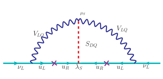
Figure 8: Feynman diagram for two-loop neutrino mass generation via VLQ and SDQ mediators, cf. Eq. (III).

The two-loop contribution to light neutrino masses in the flavor basis is given by

$${}M^{\nu}_{\alpha\beta}\ =\ 32\,\lambda^{L}_{\alpha j}m_{u_{j}}\mu_{S}(\lambda_{S}\mathcal{I})_{jk}m_{u_{k}}\lambda^{L}_{k\beta}\,,$$ (55)

where the finite part of the two-loop integral is given by

$$\mathcal{I}_{jk}\ = \ \int\frac{d^{4}k}{\left(2\pi\right)^{4}}\,\int\frac{d^{4}p}{\left(2\pi\right)^{4}}\,\frac{1}{\left(k^{2}-m^{2}_{u_{j}}\right)}\frac{1}{\left(k^{2}-M^{2}_{V_{\rm LQ}}\right)}$$ (56)

$$\quad\times\frac{1}{\left(p^{2}-m^{2}_{u_{k}}\right)}\frac{1}{\left(p^{2}-M^{2}_{V_{\rm LQ}}\right)}\frac{1}{\left(p+k\right)^{2}-M^{2}_{S_{\rm DQ}}}\,.$$

The evaluation of this loop-integral can be done following Ref. Kohda:2012sr . Assuming that the VLQ and SDQ are much heavier than the SM quarks in the loop, the loop function can be reduced to Babu:2002uu

$$\mathcal{I}_{jk}\ \simeq\ \mathcal{I}_{0}\ =\ \frac{1}{(4\pi)^{4}}\frac{1}{({\rm max}[M_{V_{\rm LQ}},M_{S_{\rm DQ}}])^{2}}\frac{\pi^{2}}{3}\widetilde{\mathcal{I}}\left(\frac{M_{S_{\rm DQ}}^{2}}{M_{V_{\rm LQ}}^{2}}\right)\,,$$ (57)

where the function $\widetilde{\mathcal{I}}(x)$ has closed-form analytic expression in the following limits:

$$\widetilde{\mathcal{I}}(x)\ =\ \left\{\begin{array}[]{ll}1+\frac{3}{\pi^{2}}\left\{(\ln x)^{2}-1\right\}&{\rm for}~{}x\gg 1\\ 1&{\rm for}~{}x\ll 1.\end{array}\right.$$ (60)

Note that here we have assumed the VLQ loops in Fig. 8 are regularized with a suitable gauge choice (for instance, the nonlinear $R_{\xi}$ gauge Gavela:1981ri ), without affecting the phenomenology discussed here. In general, vector boson propagators cause divergences that result in a bad UV behavior. Analogous to the SM case where the UV divergence in gauge boson loops are canceled by the Higgs loop, a heavy Higgs boson giving masses to the VLQs can cancel these UV divergences. However, the details depend on the specific UV-completion; see Refs. Assad:2017iib ; DiLuzio:2017vat ; Bordone:2017bld ; Calibbi:2017qbu ; Blanke:2018sro ; Ma:2012xj ; Boucenna:2014dia ; Barbieri:2017tuq ; Greljo:2018tuh ; DaRold:2019fiw for concrete examples. Ref. Deppisch:2016qqd considered two VLQs (instead of a VLQ and a SDQ as in our case) to cancel the remaining infinities contained in the Passarino-Veltman function by summing over both VLQs. In their case, the neutrino mass can be generated at one-loop level by Higgs-VLQ mixing.

Since for the flavor anomalies, we have only considered couplings to third and second generation fermions, and therefore, do not have full information on all the $\lambda^{L}_{\alpha j}$ couplings needed to fit the 3-neutrino oscillation data using Eq. (55), we will only derive an order-of-magnitude estimate for the neutrino mass constraint on the model parameters. For illustration, let us take the Scenario-I Case-III which provides the best-fit to both $b\to c\tau\bar{\nu_{\tau}}$ and $b\to s\ell\ell$ anomalies, as discussed in Section V . In this case, the best-fit values of the relevant $\lambda^{L}$ couplings, $(\lambda^{L}_{33},\lambda^{L}_{23})=(0.56,0.51)$ can be read off from Table 1 . Also recall that we have fixed the VLQ mass at $M_{V_{\rm LQ}}=1.2$ TeV for the flavor anomalies. We still have three unknowns in Eq. (55) , namely, the trilinear mass term $\mu_{S}$, Yukawa coupling $\lambda_{S}$ and the SDQ mass $M_{S_{\rm DQ}}$. As we will see in Section VIII , the $\lambda_{S}$ coupling cannot be arbitrarily large due to collider constraints from diquark searches. Similarly, the trilinear mass term $\mu_{S}$ cannot be arbitrarily large due to perturbativity constraints in the scalar sector, similar to the Zee-Babu model case Nebot:2007bc and we expect $\mu_{S}\lesssim{\rm min}(M_{V_{\rm LQ}},M_{S_{\rm DQ}})$. We will assume $\mu_{S}\ll M_{V_{\rm LQ}}<M_{S_{\rm DQ}}$ which allows us to have larger $\lambda_{S}$ couplings, while being consistent with the dijet constraints (see Section VIII). In Fig. 9 , we have shown the contours of the neutrino mass parameter $M^{\nu}_{33}$ in units of eV in the $(M_{S_{\rm DQ}},\lambda_{S})$ plane for a fixed $\mu_{S}=1.0$ MeV. For a desired neutrino mass value, increasing the value of $\mu_{S}$ will result in a smaller corresponding $\lambda_{S}$, according to Eq. (55). Here we have taken $m_{u_{j}}=m_{u_{k}}=m_{t}=173$ GeV in Eq. (55).

VIII Scalar Diquark at the LHC

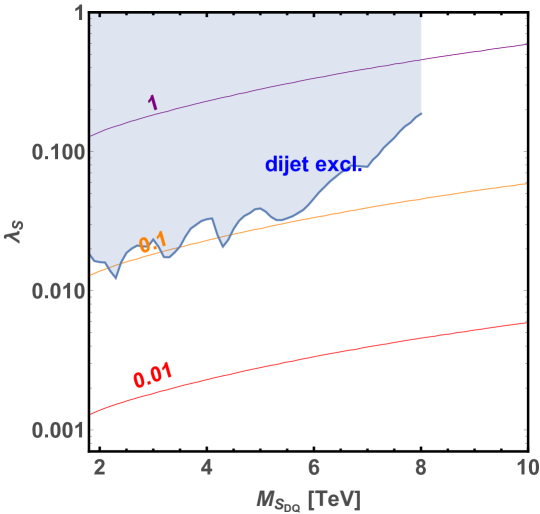
Figure 9: Contours of neutrino mass parameter $M^{\nu}_{33}$ in units of eV in the SDQ mass $M_{S_{\rm DQ}}$ versus its Yukawa coupling $\lambda_{S}$ plane. The shaded region is excluded at $95\%$ CL from a recent CMS dijet resonance search CMS-PAS-EXO-17-026 .

The new TeV-scale colored particles in our model predominantly couple to third and second-generation fermions, and offer rich phenomenology at current and future hadron colliders, such as the LHC and its high-luminosity phase, as well as future hadron colliders. The collider phenomenology of color-triplet VLQs coupling to third-generation fermions has been extensively studied; see e.g. Refs. Diaz:2017lit ; Biswas:2018snp ; Vignaroli:2018lpq ; Baker:2019sli ; Zhang:2019jwp ; Bhaskar:2020gkk . In our numerical fits for the $B$-physics anomalies, we have fixed the VLQ mass at $1.2$ TeV, which is consistent with the current LHC constraints Sirunyan:2018kzh .

On the other hand, the color-sextet SDQ introduced here to explain the neutrino mass is not constrained by the $B$-physics sector. In this section, we explore the collider constraints on the SDQ and its future detection prospects. At the LHC, the SDQ can be either singly produced by the annihilation of two up-type quarks, or pair-produced via the gluon-gluon annihilation. The single production has the advantage for relatively heavy SDQ due to the $s$-channel resonance Cakir:2005iw ; Han:2010rf , so we focus on this channel only. The single production cross section is governed by the Yukawa coupling $\lambda_{S}$ in Eq. (III), which in general has a flavor structure. For simplicity, we assume $\lambda_{S}$ to be proportional to the identity matrix, so that it couples with equal strength to $uu$, $cc$ and $tt$. Note that for the neutrino mass generation, it might suffice to have a nonzero coupling to $tt$ and $cc$ only; however, for its production at LHC, an SDQ coupling to $uu$ is desirable due to the large $u$-quark PDF inside a proton.

Once produced on-shell, the SDQ will decay back to the diquark final states. For $M_{S_{\rm DQ}}\gg 2m_{t}$, the branching ratios to all quark flavors is roughly the same; for $M_{S_{\rm DQ}}$ close to the $2m_{t}$ threshold, one has to include the phase space suppression factor of $(1-4m_{t}^{2}/M^{2}_{S_{\rm DQ}})^{3/2}$ in the $S\to tt$ partial decay rate. In our model, for $M_{S_{\rm DQ}}>2M_{V_{\rm LQ}}$, the SDQ can also decay into a pair of VLQs; however, we will choose the corresponding coupling strength $\mu_{S}$ to be small, so that the diquark decay modes are the dominant ones. A small $\mu_{S}$ is also favored by the neutrino mass constraint, if we allow for relatively large $\lambda_{S}$ values.

In Fig. 10 , we show the SDQ single production cross section (normalized to $|\lambda_{S}|^{2}=1$) times branching ratio into dijet ($uu+cc$) and ditop ($tt$) final states at $\sqrt{s}=13$ TeV LHC. These numbers were obtained at parton level using MadGraph5 Alwall:2014hca at the leading order. We have used NNPDF3.1 PDF sets AbdulKhalek:2019bux with default dynamical renormalization and factorization scales. Also shown is the current $95\%$ CL upper limit on the dijet cross section times branching ratio times acceptance from a recent CMS analysis CMS-PAS-EXO-17-026 . Comparing the dijet cross section with the corresponding CMS upper limit, one can derive an upper limit on the coupling $\lambda_{S}$ as a function of the SDQ mass, as shown by the blue shaded region in Fig. 9. We find that the dijet constraint requires $\lambda_{S}\lesssim 0.01-0.1$ for a multi-TeV SDQ.

The same-sign top pair ($tt$) final state offers a promising test of the SDQ in this model, since the SM background is very small Mohapatra:2007af ; Cao:2011ew ; Berger:2011ua ; Ebadi:2018ueq ; Cho:2019stk . The current experimental limit at $95\%$ CL from a recent ATLAS analysis Aaboud:2018xpj is shown in Fig. 10 , which only goes till $3$ TeV resonance mass. The corresponding constraint on $\lambda_{S}$ turns out to be weaker than the dijet constraint derived above. However, we expect the ditop sensitivity to improve in the high-luminosity phase and/or in the future hadron colliders.

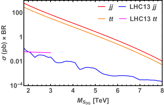
Figure 10: Cross section times branching ratio (normalized to $|\lambda_{S}|^{2}=1$) in the dijet and ditop channels from the SDQ resonance at the $\sqrt{s}=13$ TeV LHC. Also shown are the experimental upper limits at 95% CL from recent LHC dijet CMS-PAS-EXO-17-026 and same-sign top-pair Aaboud:2018xpj searches.

IX ANITA Anomaly

Recently, the ANITA collaboration has reported two anomalous upward-going ultra-high energy cosmic ray (UHECR) air shower events with deposited shower energies of $0.6\pm 0.4$ EeV Gorham:2016zah and $0.56^{+0.3}_{-0.2}$ EeV Gorham:2018ydl . This is difficult to explain within the SM framework due to the low survival rate ($\lesssim 10^{-6}$) of EeV-energy neutrinos over long chord lengths in Earth$\sim 7000$ km, even after accounting for the probability increase due to $\nu_{\tau}$ regeneration Fox:2018syq ; Romero-Wolf:2018zxt ; Reno:2019jtr ; Chipman:2019vjm . Moreover, as pointed out in Refs. Collins:2018jpg ; Shoemaker:2019xlt , the strength of isotropic cosmogenic neutrino flux needed to account for the two events is in severe tension with the upper limits set by Pierre Auger Zas:2017xdj and IceCube Aartsen:2020vir . Therefore, a NP explanation with an anisotropic astrophysical source with some exotic generation and propagation mechanism of upgoing events is desirable to solve the ANITA anomaly; see e.g. Refs. Chauhan:2018lnq ; Altmannshofer:2020axr ; Fox:2018syq ; Collins:2018jpg ; Shoemaker:2019xlt ; Cherry:2018rxj ; Huang:2018als ; Anchordoqui:2018ucj ; Heurtier:2019git ; Hooper:2019ytr ; Cline:2019snp ; Esteban:2019hcm ; Heurtier:2019rkz ; Borah:2019ciw ; Anchordoqui:2019utb ; Abdullah:2019ofw ; Esmaili:2019pcy ; Safa:2019ege .

As already pointed out in Ref. Chauhan:2018lnq , the observed ANITA events can be explained in our VLQ model framework by including a fermion singlet field $\chi({\bf 1},{\bf 1},0)$, which couples to the VLQ as given by the last term in Eq. (III). Note that this is one of the handful models that admit LQ coupling to a singlet fermion (aka sterile neutrino) Azatov:2018kzb ; Angelescu:2018tyl ; Dorsner:2016wpm . This new coupling leads to the production of $\chi$ in the neutrino interactions with up-type quarks ($u,c$) in Earth matter mediated by the VLQ, which can be resonantly enhanced for TeV-scale VLQ. This occurs for the incoming neutrino energy $E_{\nu}=M^{2}_{V_{\rm LQ}}/2m_{N}x$, where $m_{N}\simeq 1$ GeV is the nucleon mass and $x$ is the Bjorken scaling variable, which has an average value of $\sim 10^{-3}$ for these deep inelastic scattering processes. The $\chi$ being a SM-singlet can in principle be long-lived and traverses the required chord length before decaying via the same interactions into a ${D}_{s}$ meson and a charged lepton; see Fig. 11 . We will assume that the charged lepton produced from the $\chi$ decay is a tau lepton, which comes from the $\lambda^{L}_{23}$ coupling of the VLQ that is also relevant for the $B$-anomalies discussed above.

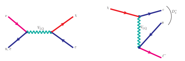
Figure 11: VLQ mediated Feynman diagram for neutrino-quark interaction resulting into production of a long-lived particle $\chi$ (left-panel) and the decay of this long lived particle $\chi$ into $D^{+}_{s}$ $\ell^{-}$ (right panel).

After integrating out the VLQ and performing Fierz transformation, the relevant interaction Lagrangian obtained from Eq. (III) becomes

$$\mathcal{L}\ \supset\ \frac{2(\lambda_{\chi})_{\alpha}\lambda^{L}_{ij}}{M_{V_{\rm LQ}^{2}}}\left(\bar{u}_{R\alpha}d_{iL}\right)\left(\bar{\ell}_{jL}\chi_{R}\right)\,,$$ (61)

where the generation indices are as follows: $\alpha=1,2,3$ and $i,j=2,3$. Using Eq. (61), the rate of $\chi\to\tau D_{s}$ decay mode is given by

$$\Gamma(\chi\to\tau D_{s}^{+})\ =\ \frac{\lambda^{1/2}(M_{\chi}^{2},M_{D_{s}^{+}}^{2},m_{\tau}^{2})}{16\pi M_{\chi}^{3}}\left(\frac{\lambda_{\chi}\lambda_{23}^{L}}{M_{V_{\rm LQ}}^{2}}\right)\left(\frac{M_{D_{s}^{+}}^{2}f_{D_{s}^{+}}}{m_{c}+m_{s}}\right)^{2}\left(M_{\chi}^{2}-M_{D_{s}^{+}}^{2}+m_{\tau}^{2}\right)\,,$$ (62)

where we have denoted $(\lambda_{\chi})_{2}$ simply as $\lambda_{\chi}$. The masses of $D_{s}^{+}$ meson and $\tau$ lepton are taken from PDG Tanabashi:2018oca and the decay constant $f_{D_{s}^{+}}=257.86$ MeV. We simulate the production of $\chi$ by implementing our model file into MadGraph5 Alwall:2014hca at the leading order and using the NNPDF3.1 PDF sets AbdulKhalek:2019bux . This is followed by the decay of $\chi$ given by Eq. (62) to estimate the event rate at ANITA Collins:2018jpg :

$$N\ =\ \int dE_{\nu}\ \langle A_{\rm eff}\cdot\Delta\Omega\rangle\cdot T\cdot\Phi_{\nu}\,,$$ (63)

where $T=53$ days for the total effective exposure time, $\Phi_{\nu}=2\times 10^{-20}\rm{(GeV\cdot cm^{2}\cdot s\cdot sr)^{-1}}$ for the cosmic neutrino flux, and $\langle A_{\rm eff}\cdot\Delta\Omega\rangle$ is the effective area integrated over the relevant solid angle, averaged over the probability for interaction and decay to happen over the specified geometry. The effective area contains all the information of the geometry, decay width of $\chi$ and the cross section for the $\chi$ production; see Ref. Collins:2018jpg for the explicit expression for an analogous bino production in supersymmetry. In particular, the mean lifetime of the $\chi$ particle should be fixed at around 0.022 s in the laboratory frame in order to achieve a chord length of $\sim 7000$ km inside the Earth, as required by the ANITA observation. Such long lifetime ensures that there are no direct laboratory constraints on the $\chi$ couplings. From Eq. (63), we know that the overall event number $N$ is a function of $m_{\chi}$ and $\lambda_{\chi}$ for a given VLQ mass. Therefore, comparing the simulated event numbers with the ANITA observation of two anomalous events gives us the best-fit parameter region at a given CL. This is shown in Fig. 12 , where the dark and light blue-shaded regions can explain the ANITA events at $2\sigma$ and $3\sigma$ CL respectively for $M_{V_{\rm LQ}}=1.2$ TeV. The vertical grey-shaded region is kinematically forbidden for the $\chi$ decay shown in the right panel of Fig. 11. Note that our results for the ANITA-preferred region in Fig. 12 are slightly different from those given in Ref. Chauhan:2018lnq . We also include the $D^{0}-\overline{D}^{0}$ mixing constraint, as discussed below.

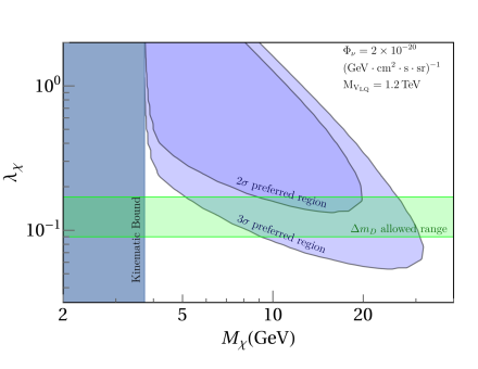
Figure 12: The $2\sigma$ and $3\sigma$ preferred region in the $(M_{\chi},\lambda_{\chi})$ parameter space to explain the ANITA anomalous events in our VLQ model. The green-shaded region is allowed by the $D^{0}-\overline{D}^{0}$ mixing constraint. In the vertical grey-shaded region, the $\chi$ decay shown in the right panel of Fig. 11 is not kinematically allowed.

In presence of the singlet $\chi$, there will be a new contribution to the $D^{0}-\overline{D}^{0}$ mass difference from the box diagrams with the VLQ and $\chi$ flowing in the loop, as shown in Fig. 13.

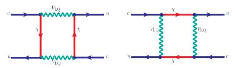
Figure 13: Feynman diagram for one loop box diagram for $D^{0}-\overline{D}^{0}$ mixing mediated by the singlet $\chi$ and the VLQ.

The effective Hamiltonian for $D^{0}-\overline{D}^{0}$ mixing in the presence of VLQ is

$${\cal H}^{\rm NP}_{\rm eff}\ =\ C_{D\overline{D}}(\bar{u}\gamma^{\mu}(1-\gamma_{5})c)(\bar{u}\gamma^{\mu}(1-\gamma_{5})c)\,,$$ (64)

where the NP Wilson coefficient is given as

$$C_{D\overline{D}}\ =\ \frac{\lambda_{\chi}^{4}}{128\pi^{2}M_{V_{\rm LQ}}^{2}}F(x_{\chi},x_{\chi}),$$ (65)

with $x_{\chi}=M_{\chi}^{2}/M_{V_{\rm LQ}}^{2}$ and the loop function

$$F(x_{i},x_{j}) \ =\ \frac{1}{(1-x_{i})(1-x_{j})}+\frac{x_{i}^{2}\log x_{i}}{(1-x_{i})^{2}(x_{i}-x_{j})}+\frac{x_{j}^{2}\log x_{j}}{(1-x_{j})^{2}(x_{j}-x_{i})}.$$ (66)

The SM contribution to the mass difference is negligible and the corresponding measured value is given by Tanabashi:2018oca

$$\Delta M_{D}\ =\ 0.0095^{+0.0041}_{-0.0044}~{}{\rm ps}^{-1}.$$ (67)

The green-shaded region in Fig. 12 shows the allowed parameter space from this constraint.

The presence of $\chi$ also leads to an additional contribution to the $B_{c}^{+}\to\tau^{+}\nu$ process, via a diagram similar to the right-panel of Fig. 11 (with $s$ replaced by $b$), since the $\chi$ practically behaves like a neutrino for the energies involved in the $B$-decays. The corresponding branching ratio is given by

$${\rm BR}(B_{c}^{+}\to\ell^{+}\chi)\ =\ \tau_{B_{c}}\frac{\lambda(M_{B_{c}}^{2},m_{\ell}^{2},M_{\chi}^{2})^{1/2}}{8\pi M_{B_{c}}^{3}}\left(\frac{\lambda_{\chi}\lambda_{3j}^{L}}{M_{V_{\rm LQ}}^{2}}\right)^{2}\left(\frac{M_{B_{c}^{+}}^{2}f_{B_{c}^{+}}}{m_{b}+m_{c}}\right)^{2}$$ (68)

$$\quad\times\left(M_{B_{c}}^{2}-m_{\ell}^{2}-M_{\chi}^{2}\right)\,.$$

For $M_{B_{c}}=6.25$ GeV and $m_{\tau}=1.77~{}(m_{\mu}=0.106)$ GeV Tanabashi:2018oca , the maximum mass value of $\chi$ for which the $B_{c}^{+}\to\ell^{+}\chi$ process can occur kinematically is $M_{\chi}=4.47~{}(6.144)$ GeV. However, from Fig. 12 , we see that the overlap between the ANITA and $\Delta m_{D}$ preferred regions occurs only between $M_{\chi}=[6,30]$ GeV. Hence, the $B_{c}^{+}\to\tau^{+}\chi$ decay is not relevant here.

X Conclusion

The recently observed various flavor anomalies in the CC and NC mediated semileptonic $B$ meson decays may be considered as one of the most compelling hints of NP at the TeV scale. To explain these intriguing set of discrepancies in a coherent manner using a single framework is a challenging task, as the NP scales involved in the CC and NC sectors are significantly different from each other. To achieve this goal, in this article we considered a minimal extension of the SM with an additional TeV scale vector leptoquark, which transforms as $({\bf 3},{\bf 1},2/3)$ under the SM gauge group. The interesting feature of this model framework is that both the transitions $b\to c\tau\bar{\nu}_{\tau}$ and $b\to s\ell^{+}\ell^{-}$ occur at the tree level through the exchange of the VLQ, and it also provides the required NP contributions to simultaneously resolve the anomalies. Assuming that NP can couple only to second and third generation fermions and taking into account all possible chiral couplings ($LL,RR,LR,RL$) of the SM quarks and charged leptons with the LQ, we performed a global fit to constrain the NP parameters by using the observables associated with $b\to s\mu^{-}\mu^{+}(\tau^{-}\tau^{+})$ and $b\to c\tau\bar{\nu}_{\tau}$ transitions. We find that for a TeV-scale VLQ, only the $LL$-type couplings can simultaneously explain both $b\to s\ell^{+}\ell^{-}$ and $b\to c\tau\bar{\nu}_{\tau}$ anomalies with a $\chi^{2}_{\rm min}/{\rm d.o.f.}<1$. The model predictions for lepton flavor violating $B$-meson, $\Upsilon(nS)$ and $\tau$-lepton decays (see Table 2) can be used to test this scenario in the future $B$-physics experiments, such as LHCb upgrade and Belle-II.

In addition, augmenting the VLQ model with a color-sextet SDQ can explain the neutrino mass at two-loop level (see Section VII). We discussed the LHC constraints on the SDQ mass and Yukawa coupling with up-type quarks, and identified the same-sign top-pair production as an excellent probe of this scenario for a multi-TeV SDQ in the future high-energy collider experiments, such as high-luminosity LHC (see Section VIII). Further, adding a GeV-scale SM-singlet fermion to the VLQ model can also explain the ANITA anomalous upgoing events. It was shown to be consistent with the $D^{0}-\overline{D^{0}}$ mixing constraint (see Fig. 12). In summary, we have proposed a unified explanation of the flavor anomalies, radiative neutrino mass and ANITA events. Different aspects of the model can be tested in future collider and $B$-physics experiments.

Appendix A Experimental data used in fit

The experimental measured central values, statistical and systematic uncertainties of all the observables used in our analysis are presented in the following Tables 3-7 .

Decay processes	$q^{2}$ bin (${\rm GeV}^{2}$)	$d{\rm BR}/dq^{2}\times 10^{-7}~{}({\rm GeV}^{-2})$
$B^{+}\to K^{+}\mu^{+}\mu^{-}$	$0.10<q^{2}<0.98$	$0.332\pm 0.018\pm 0.017$
	$1.1<q^{2}<2.0$	$0.233\pm 0.015\pm 0.012$
	$2.0<q^{2}<3.0$	$0.282\pm 0.016\pm 0.014$
	$3.0<q^{2}<4.0$	$0.254\pm 0.015\pm 0.013$
	$4.0<q^{2}<5.0$	$0.221\pm 0.014\pm 0.011$
	$5.0<q^{2}<6.0$	$0.231\pm 0.014\pm 0.012$
	$1.1<q^{2}<6.0$	$0.242\pm 0.007\pm 0.012$
$B^{0}\to K^{0}\mu^{+}\mu^{-}$	$0.10<q^{2}<2.0$	$0.122^{+0.059}_{-0.052}\pm 0.006$
	$2.0<q^{2}<4.0$	$0.187^{+0.055}_{-0.049}\pm 0.009$
	$4.0<q^{2}<6.0$	$0.173^{+0.053}_{-0.048}\pm 0.009$
	$1.1<q^{2}<6.0$	$0.187^{+0.035}_{-0.032}\pm 0.009$
$B^{+}\to K^{*+}\mu^{+}\mu^{-}$	$0.10<q^{2}<2.0$	$0.592^{+0.144}_{-0.130}\pm 0.004$
	$2.0<q^{2}<4.0$	$0.559^{+0.159}_{-0.144}\pm 0.038$
	$4.0<q^{2}<6.0$	$0.249^{+0.110}_{-0.096}\pm 0.017$
	$1.1<q^{2}<6.0$	$0.366^{+0.083}_{-0.076}\pm 0.026$
$B^{0}\to K^{*0}\mu^{+}\mu^{-}$	$0.10<q^{2}<0.98$	$1.016^{+0.067}_{-0.073}\pm 0.029\pm 0.069$
	$1.1<q^{2}<2.5$	$0.326^{+0.032}_{-0.031}\pm 0.010\pm 0.022$
	$2.5<q^{2}<4.0$	$0.334^{+0.031}_{-0.033}\pm 0.009\pm 0.023$
	$4.0<q^{2}<6.0$	$0.354^{+0.027}_{-0.026}\pm 0.009\pm 0.024$
	$1.1<q^{2}<6.0$	$0.342^{+0.017}_{-0.017}\pm 0.009\pm 0.023$
$B_{s}\to\phi\mu^{+}\mu^{-}$	$0.10<q^{2}<2.0$	$0.585^{+0.073}_{-0.069}\pm 0.014\pm 0.044$
	$2.0<q^{2}<5.0$	$0.256^{+0.042}_{-0.039}\pm 0.006\pm 0.019$
	$1.0<q^{2}<6.0$	$0.258^{+0.033}_{-0.031}\pm 0.008\pm 0.019$

Table 3: Experimental measurements on the differential branching ratios of $B^{+}\to K^{+}\mu^{+}\mu^{-}$ Aaij:2014pli , $B^{0}\to K^{0}\mu^{+}\mu^{-}$ Aaij:2014pli , $B^{+}\to K^{*+}\mu^{+}\mu^{-}$ Aaij:2014pli , $B^{0}\to K^{*0}\mu^{+}\mu^{-}$ Aaij:2015oid and $B_{s}\to\phi\mu^{+}\mu^{-}$ Aaij:2015esa processes in bins of $q^{2}$. Here the first uncertainties are statistical, the second are systematic and the third arise due to the uncertainty on the $B^{0}\to J/\psi K^{*0}$ ($B_{s}^{0}\to J/\psi\phi$) and $J/\psi\to\mu^{+}\mu^{-}$.

Observable	$q^{2}$ bin (${\rm GeV}^{2}$)	Measurement	Observable	$q^{2}$ bin (${\rm GeV}^{2}$)	Measurement
$F_{L}$	$0.10<q^{2}<0.98$	$0.242^{+0.058}_{-0.056}\pm 0.026$	$A_{FB}$	$0.10<q^{2}<0.98$	$-0.138^{+0.095}_{-0.092}\pm 0.072$
	$1.1<q^{2}<2.0$	$0.768^{+0.141}_{-0.130}\pm 0.025$		$1.1<q^{2}<2.0$	$-0.333^{+0.115}_{-0.130}\pm 0.012$
	$2.0<q^{2}<3.0$	$0.690^{+0.113}_{-0.082}\pm 0.023$		$2.0<q^{2}<3.0$	$-0.158^{+0.080}_{-0.090}\pm 0.008$
	$3.0<q^{2}<4.0$	$0.873^{+0.154}_{-0.105}\pm 0.023$		$3.0<q^{2}<4.0$	$-0.041^{+0.091}_{-0.091}\pm 0.002$
	$4.0<q^{2}<5.0$	$0.899^{+0.106}_{-0.104}\pm 0.023$		$4.0<q^{2}<5.0$	$0.052^{+0.080}_{-0.080}\pm 0.004$
	$5.0<q^{2}<6.0$	$0.644^{+0.130}_{-0.121}\pm 0.025$		$5.0<q^{2}<6.0$	$0.057^{+0.094}_{-0.090}\pm 0.006$
	$1.1<q^{2}<6.0$	$0.690^{+0.035}_{-0.036}\pm 0.017$		$1.1<q^{2}<6.0$	$-0.075^{+0.032}_{-0.034}\pm 0.007$
$S_{3}$	$0.10<q^{2}<0.98$	$-0.014^{+0.059}_{-0.060}\pm 0.008$	$S_{4}$	$0.10<q^{2}<0.98$	$0.039^{+0.091}_{-0.090}\pm 0.015$
	$1.1<q^{2}<2.0$	$0.065^{+0.137}_{-0.127}\pm 0.007$		$1.1<q^{2}<2.0$	$0.127^{+0.190}_{-0.180}\pm 0.027$
	$2.0<q^{2}<3.0$	$0.006^{+0.100}_{-0.100}\pm 0.007$		$2.0<q^{2}<3.0$	$-0.339^{+0.115}_{-0.140}\pm 0.041$
	$3.0<q^{2}<4.0$	$0.078^{+0.131}_{-0.122}\pm 0.008$		$3.0<q^{2}<4.0$	$-0.046^{+0.193}_{-0.196}\pm 0.046$
	$4.0<q^{2}<5.0$	$0.200^{+0.101}_{-0.097}\pm 0.007$		$4.0<q^{2}<5.0$	$-0.148^{+0.154}_{-0.154}\pm 0.047$
	$5.0<q^{2}<6.0$	$-0.122^{+0.119}_{-0.126}\pm 0.009$		$5.0<q^{2}<6.0$	$-0.273^{+0.174}_{-0.184}\pm 0.048$
	$1.1<q^{2}<6.0$	$0.012^{+0.038}_{-0.038}\pm 0.004$		$1.1<q^{2}<6.0$	$-0.155^{+0.057}_{-0.056}\pm 0.004$
$S_{5}$	$0.10<q^{2}<0.98$	$0.129^{+0.068}_{-0.068}\pm 0.011$	$S_{7}$	$0.10<q^{2}<0.98$	$0.038^{+0.063}_{-0.062}\pm 0.009$
	$1.1<q^{2}<2.0$	$0.286^{+0.168}_{-0.172}\pm 0.009$		$1.1<q^{2}<2.0$	$-0.293^{+0.180}_{-0.176}\pm 0.005$
	$2.0<q^{2}<3.0$	$0.206^{+0.131}_{-0.115}\pm 0.009$		$2.0<q^{2}<3.0$	$-0.252^{+0.127}_{-0.151}\pm 0.002$
	$3.0<q^{2}<4.0$	$-0.110^{+0.163}_{-0.169}\pm 0.004$		$3.0<q^{2}<4.0$	$0.171^{+0.175}_{-0.158}\pm 0.002$
	$4.0<q^{2}<5.0$	$-0.306^{+0.138}_{-0.141}\pm 0.004$		$4.0<q^{2}<5.0$	$-0.082^{+0.129}_{-0.128}\pm 0.001$
	$5.0<q^{2}<6.0$	$-0.095^{+0.137}_{-0.142}\pm 0.004$		$5.0<q^{2}<6.0$	$0.038^{+0.135}_{-0.135}\pm 0.002$
	$1.1<q^{2}<6.0$	$-0.023^{+0.050}_{-0.049}\pm 0.005$		$1.1<q^{2}<6.0$	$-0.077^{+0.050}_{-0.049}\pm 0.006$
$S_{8}$	$0.10<q^{2}<0.98$	$0.063^{+0.079}_{-0.080}\pm 0.009$	$S_{9}$	$0.10<q^{2}<0.98$	$-0.113^{+0.061}_{-0.063}\pm 0.004$
	$1.1<q^{2}<2.0$	$-0.114^{+0.185}_{-0.196}\pm 0.006$		$1.1<q^{2}<2.0$	$-0.110^{+0.140}_{-0.138}\pm 0.001$
	$2.0<q^{2}<3.0$	$-0.176^{+0.149}_{-0.165}\pm 0.006$		$2.0<q^{2}<3.0$	$-0.000^{+0.100}_{-0.102}\pm 0.003$
	$3.0<q^{2}<4.0$	$0.097^{+0.189}_{-0.184}\pm 0.002$		$3.0<q^{2}<4.0$	$-0.203^{+0.112}_{-0.132}\pm 0.002$
	$4.0<q^{2}<5.0$	$0.107^{+0.144}_{-0.146}\pm 0.003$		$4.0<q^{2}<5.0$	$0.181^{+0.105}_{-0.099}\pm 0.001$
	$5.0<q^{2}<6.0$	$-0.037^{+0.160}_{-0.159}\pm 0.003$		$5.0<q^{2}<6.0$	$-0.080^{+0.117}_{-0.120}\pm 0.001$
	$1.1<q^{2}<6.0$	$0.028^{+0.058}_{-0.057}\pm 0.008$		$1.1<q^{2}<6.0$	$0.064^{+0.042}_{-0.041}\pm 0.004$

Table 4: CP-averaged angular observables of $B^{0}\to K^{*0}\mu^{+}\mu^{-}$ process in bins of $q^{2}$, evaluated using the method of moments Aaij:2015oid . We have used the $q^{2}\in[1.1,6.0]$ bin result evaluated by the unbinned maximum likelihood fit. Here the first uncertainties are statistical and the second are systematic.

Observable	$q^{2}$ bin (${\rm GeV}^{2}$)	Measurement	Observable	$q^{2}$ bin (${\rm GeV}^{2}$)	Measurement
$A_{3}$	$0.10<q^{2}<0.98$	$-0.040^{+0.059}_{-0.061}\pm 0.007$	$A_{4}$	$0.10<q^{2}<0.98$	$-0.047^{+0.090}_{-0.092}\pm 0.013$
	$1.1<q^{2}<2.0$	$-0.134^{+0.126}_{-0.136}\pm 0.003$		$1.1<q^{2}<2.0$	$0.283^{+0.191}_{-0.181}\pm 0.028$
	$2.0<q^{2}<3.0$	$-0.018^{+0.101}_{-0.100}\pm 0.001$		$2.0<q^{2}<3.0$	$-0.261^{+0.146}_{-0.123}\pm 0.042$
	$3.0<q^{2}<4.0$	$-0.118^{+0.120}_{-0.132}\pm 0.007$		$3.0<q^{2}<4.0$	$0.002^{+0.194}_{-0.196}\pm 0.045$
	$4.0<q^{2}<5.0$	$-0.064^{+0.098}_{-0.098}\pm 0.005$		$4.0<q^{2}<5.0$	$0.076^{+0.155}_{-0.154}\pm 0.047$
	$5.0<q^{2}<6.0$	$-0.076^{+0.119}_{-0.122}\pm 0.004$		$5.0<q^{2}<6.0$	$-0.457^{+0.174}_{-0.187}\pm 0.048$
	$1.1<q^{2}<6.0$	$-0.173^{+0.070}_{-0.079}\pm 0.006$		$1.1<q^{2}<6.0$	$-0.168^{+0.086}_{-0.085}\pm 0.008$
$A_{5}$	$0.10<q^{2}<0.98$	$-0.008^{+0.066}_{-0.066}\pm 0.011$	$A_{7}$	$0.10<q^{2}<0.98$	$0.112^{+0.064}_{-0.062}\pm 0.010$
	$1.1<q^{2}<2.0$	$-0.110^{+0.166}_{-0.176}\pm 0.008$		$1.1<q^{2}<2.0$	$-0.193^{+0.167}_{-0.200}\pm 0.006$
	$2.0<q^{2}<3.0$	$0.028^{+0.124}_{-0.120}\pm 0.008$		$2.0<q^{2}<3.0$	$-0.162^{+0.130}_{-0.144}\pm 0.003$
	$3.0<q^{2}<4.0$	$0.015^{+0.167}_{-0.168}\pm 0.005$		$3.0<q^{2}<4.0$	$-0.004^{+0.165}_{-0.12}\pm 0.003$
	$4.0<q^{2}<5.0$	$-0.051^{+0.143}_{-0.142}\pm 0.005$		$4.0<q^{2}<5.0$	$-0.146^{+0.13}_{-0.13}\pm 0.003$
	$5.0<q^{2}<6.0$	$-0.011^{+0.139}_{-0.139}\pm 0.006$		$5.0<q^{2}<6.0$	$0.116^{+0.124}_{-0.121}\pm 0.003$
	$1.1<q^{2}<6.0$	$-0.059^{+0.071}_{-0.073}\pm 0.011$		$1.1<q^{2}<6.0$	$0.041^{+0.083}_{-0.082}\pm 0.004$
$A_{8}$	$0.10<q^{2}<0.98$	$0.021^{+0.080}_{-0.080}\pm 0.012$	$A_{9}$	$0.10<q^{2}<0.98$	$0.043^{+0.062}_{-0.062}\pm 0.009$
	$1.1<q^{2}<2.0$	$0.130^{+0.203}_{-0.180}\pm 0.008$		$1.1<q^{2}<2.0$	$-0.126^{+0.136}_{-0.153}\pm 0.010$
	$2.0<q^{2}<3.0$	$-0.060^{+0.152}_{-0.161}\pm 0.006$		$2.0<q^{2}<3.0$	$0.013^{+0.102}_{-0.101}\pm 0.007$
	$3.0<q^{2}<4.0$	$0.005^{+0.188}_{-0.185}\pm 0.003$		$3.0<q^{2}<4.0$	$-0.129^{+0.115}_{-0.125}\pm 0.003$
	$4.0<q^{2}<5.0$	$0.183^{+0.150}_{-0.146}\pm 0.001$		$4.0<q^{2}<5.0$	$0.160^{+0.103}_{-0.100}\pm 0.008$
	$5.0<q^{2}<6.0$	$-0.195^{+0.156}_{-0.167}\pm 0.007$		$5.0<q^{2}<6.0$	$-0.001^{+0.118}_{-0.120}\pm 0.002$
	$1.1<q^{2}<6.0$	$0.004^{+0.093}_{-0.095}\pm 0.005$		$1.1<q^{2}<6.0$	$0.062^{+0.078}_{-0.072}\pm 0.004$

Table 5: CP asymmetries of $B^{0}\to K^{*0}\mu^{+}\mu^{-}$ process in bins of $q^{2}$, evaluated using the method of moments Aaij:2015oid . We have used the $q^{2}\in[1.1,6.0]$ bin result evaluated by the unbinned maximum likelihood fit. Here the first uncertainties are statistical and the second are systematic.

Observable	$q^{2}$ bin (${\rm GeV}^{2}$)	Measurement	Observable	$q^{2}$ bin (${\rm GeV}^{2}$)	Measurement
$P_{1}$	$0.10<q^{2}<0.98$	$-0.038^{+0.157}_{-0.158}\pm 0.020$	$P_{2}$	$0.10<q^{2}<0.98$	$-0.119^{+0.080}_{-0.081}\pm 0.063$
	$1.1<q^{2}<2.0$	$0.439^{+1.916}_{-1.013}\pm 0.012$		$1.1<q^{2}<2.0$	$-0.667^{+0.149}_{-1.939}\pm 0.017$
	$2.0<q^{2}<3.0$	$0.055^{+0.677}_{-0.756}\pm 0.007$		$2.0<q^{2}<3.0$	$-0.323^{+0.147}_{-0.316}\pm 0.033$
	$3.0<q^{2}<4.0$	$0.421^{+18.35}_{-1.190}\pm 0.018$		$3.0<q^{2}<4.0$	$-0.117^{+0.485}_{-4.435}\pm 0.015$
	$4.0<q^{2}<5.0$	$2.296^{+17.71}_{-0.694}\pm 0.024$		$4.0<q^{2}<5.0$	$0.174^{+3.034}_{-0.376}\pm 0.010$
	$5.0<q^{2}<6.0$	$-0.540^{+0.521}_{-1.100}\pm 0.025$		$5.0<q^{2}<6.0$	$0.089^{+0.227}_{-0.155}\pm 0.012$
	$1.1<q^{2}<6.0$	$0.080^{+0.248}_{-0.245}\pm 0.044$		$1.1<q^{2}<6.0$	$-0.162^{+0.072}_{-0.073}\pm 0.010$
$P_{3}$	$0.10<q^{2}<0.98$	$0.147^{+0.086}_{-0.080}\pm 0.005$	$P_{4}^{\prime}$	$0.10<q^{2}<0.98$	$0.086^{+0.221}_{-0.209}\pm 0.026$
	$1.1<q^{2}<2.0$	$0.363^{+1.088}_{-0.506}\pm 0.001$		$1.1<q^{2}<2.0$	$-0.266^{+0.648}_{-0.406}\pm 0.057$
	$2.0<q^{2}<3.0$	$0.005^{+0.362}_{-0.364}\pm 0.012$		$2.0<q^{2}<3.0$	$-0.765^{+0.271}_{-0.359}\pm 0.099$
	$3.0<q^{2}<4.0$	$0.905^{+17.51}_{-0.258}\pm 0.009$		$3.0<q^{2}<4.0$	$-0.134^{+0.810}_{-1.343}\pm 0.108$
	$4.0<q^{2}<5.0$	$-0.801^{+0.221}_{-17.42}\pm 0.007$		$4.0<q^{2}<5.0$	$-0.415^{+0.438}_{-1.911}\pm 0.104$
	$5.0<q^{2}<6.0$	$0.178^{+0.465}_{-0.286}\pm 0.007$		$5.0<q^{2}<6.0$	$-0.561^{+0.345}_{-0.465}\pm 0.101$
	$1.1<q^{2}<6.0$	$0.205^{+0.135}_{-0.134}\pm 0.017$		$1.1<q^{2}<6.0$	$-0.336^{+0.124}_{-0.122}\pm 0.012$
$P_{5}^{\prime}$	$0.10<q^{2}<0.98$	$0.300^{+0.171}_{-0.152}\pm 0.023$	$P_{6}^{\prime}$	$0.10<q^{2}<0.98$	$0.086^{+0.152}_{-0.145}\pm 0.024$
	$1.1<q^{2}<2.0$	$-0.632^{+0.347}_{-0.753}\pm 0.009$		$1.1<q^{2}<2.0$	$-0.244^{+0.433}_{-0.645}\pm 0.012$
	$2.0<q^{2}<3.0$	$-0.176^{+0.149}_{-0.165}\pm 0.006$		$2.0<q^{2}<3.0$	$-0.000^{+0.100}_{-0.102}\pm 0.003$
	$3.0<q^{2}<4.0$	$-0.549^{+0.276}_{-0.393}\pm 0.005$		$3.0<q^{2}<4.0$	$-0.393^{+0.332}_{-0.388}\pm 0.002$
	$4.0<q^{2}<5.0$	$0.449^{+19.04}_{-0.397}\pm 0.007$		$4.0<q^{2}<5.0$	$0.303^{+1.394}_{-0.719}\pm 0.006$
	$5.0<q^{2}<6.0$	$-0.799^{+0.266}_{-18.19}\pm 0.022$		$5.0<q^{2}<6.0$	$-0.215^{+0.397}_{-1.243}\pm 0.006$
	$1.1<q^{2}<6.0$	$-0.049^{+0.107}_{-0.108}\pm 0.014$		$1.1<q^{2}<6.0$	$-0.166^{+0.108}_{-0.108}\pm 0.021$
$P_{8}^{\prime}$	$0.10<q^{2}<0.98$	$0.143^{+0.195}_{-0.184}\pm 0.022$
	$1.1<q^{2}<2.0$	$-0.244^{+0.433}_{-0.645}\pm 0.012$
	$2.0<q^{2}<3.0$	$-0.393^{+0.332}_{-0.388}\pm 0.002$
	$3.0<q^{2}<4.0$	$0.303^{+1.394}_{-0.719}\pm 0.006$
	$4.0<q^{2}<5.0$	$0.293^{+1.522}_{-0.441}\pm 0.006$
	$5.0<q^{2}<6.0$	$-0.068^{+0.338}_{-0.372}\pm 0.006$
	$1.1<q^{2}<6.0$	$0.060^{+0.122}_{-0.124}\pm 0.009$

Table 6: Form-factor-independent optimized observables of $B^{0}\to K^{*0}\mu^{+}\mu^{-}$ process in bins of $q^{2}$, evaluated using the method of moments Aaij:2015oid . We have used the $q^{2}\in[1.1,6.0]$ bin result evaluated by the unbinned maximum likelihood fit. Here the first uncertainties are statistical and the second are systematic.

Observables	$q^{2}$ bin (${\rm GeV}^{2}$)	Measurement	Observables	$q^{2}$ bin (${\rm GeV}^{2}$)	Measurement
$F_{L}$	$0.10<q^{2}<2.0$	$0.20^{+0.08}_{-0.09}\pm 0.02$	$S_{3}$	$0.10<q^{2}<2.0$	$-0.05^{+0.13}_{-0.13}\pm 0.01$
	$2.0<q^{2}<5.0$	$0.69^{+0.16}_{-0.13}\pm 0.03$		$2.0<q^{2}<5.0$	$-0.06^{+0.19}_{-0.23}\pm 0.01$
	$1.0<q^{2}<6.0$	$0.63^{+0.09}_{-0.09}\pm 0.03$		$1.0<q^{2}<6.0$	$-0.02^{+0.12}_{-0.13}\pm 0.01$
$S_{4}$	$0.10<q^{2}<2.0$	$0.27^{+0.28}_{-0.18}\pm 0.015$	$S_{7}$	$0.10<q^{2}<2.0$	$0.04^{+0.12}_{-0.12}\pm 0.0$
	$2.0<q^{2}<5.0$	$-0.47^{+0.30}_{-0.44}\pm 0.01$		$2.0<q^{2}<5.0$	$-0.03^{+0.18}_{-0.23}\pm 0.01$
	$1.0<q^{2}<6.0$	$-0.19^{+0.14}_{-0.13}\pm 0.01$		$1.0<q^{2}<6.0$	$-0.03^{+0.14}_{-0.14}\pm 0.00$
$A_{5}$	$0.10<q^{2}<2.0$	$-0.02^{+0.13}_{-0.13}\pm 0.00$	$A_{6}$	$0.10<q^{2}<2.0$	$-0.19^{+0.15}_{-0.15}\pm 0.01$
	$2.0<q^{2}<5.0$	$0.09^{+0.28}_{-0.22}\pm 0.01$		$2.0<q^{2}<5.0$	$0.09^{+0.20}_{-0.19}\pm 0.02$
	$1.0<q^{2}<6.0$	$0.20^{+0.13}_{-0.13}\pm 0.00$		$1.0<q^{2}<6.0$	$0.08^{+0.12}_{-0.11}\pm 0.01$
$A_{8}$	$0.10<q^{2}<2.0$	$0.10^{+0.14}_{-0.14}\pm 0.00$	$A_{9}$	$0.10<q^{2}<2.0$	$0.03^{+0.14}_{-0.14}\pm 0.01$
	$2.0<q^{2}<5.0$	$0.19^{+0.26}_{-0.21}\pm 0.01$		$2.0<q^{2}<5.0$	$-0.13^{+0.24}_{-0.30}\pm 0.01$
	$1.0<q^{2}<6.0$	$-0.00^{+0.15}_{-0.17}\pm 0.00$		$1.0<q^{2}<6.0$	$-0.01^{+0.13}_{-0.13}\pm 0.01$

Table 7: CP-averaged angular observables and CP asymmetries of $B_{s}\to\phi\mu^{+}\mu^{-}$ process in bins of $q^{2}$, evaluated using the method of moments Aaij:2015esa . Here the first uncertainties are statistical and the second are systematic.

Appendix B $\boldsymbol{B\to Kl_{i}l_{j}}$

The matrix elements of the various hadronic currents between the $B$ meson and the $K$ meson can be parameterized in terms of the form factors $f_{+}$ and $f_{0}$ as Bobeth:2007dw

$$\langle K(p_{K})|\bar{s}\gamma_{\mu}b|\bar{B}(p_{B})\rangle=(2p_{B}-q)_{\mu}f_{+}(q^{2})+\frac{M_{B}^{2}-M_{K}^{2}}{q^{2}}q_{\mu}[f_{0}(q^{2})-f_{+}(q^{2})]\,.$$ (69)

The coefficients $J_{i}$ appearing in the differential branching ratio of $B\to K\ell_{i}\ell_{j}$ [Eq. (30)] are given by Duraisamy:2016gsd

$$J_{1} \ =\ 4\Bigg{[}\left(1-\frac{(m_{i}-m_{j})^{2}}{q^{2}}\right)\frac{1}{3}\left(2q^{2}+\left(m_{i}+m_{j}\right)^{2}\right)|H_{V}^{0}|^{2}$$

$$\quad+\frac{(m_{i}-m_{j})^{2}}{q^{2}}\left(q^{2}-\left(m_{i}+m_{j}\right)^{2}\right)|H_{V}^{t}|^{2}\Bigg{]},$$

$$J_{2} \ =\ 4\Bigg{[}\left(1-\frac{(m_{i}+m_{j})^{2}}{q^{2}}\right)\frac{1}{3}\left(2q^{2}+\left(m_{i}-m_{j}\right)^{2}\right)|H_{A}^{0}|^{2}$$

$$\quad+\frac{(m_{i}+m_{j})^{2}}{q^{2}}\left(q^{2}-\left(m_{i}-m_{j}\right)^{2}\right)|H_{A}^{t}|^{2}\Bigg{]},$$

$$J_{3} \ =\ 4\left[q^{2}-(m_{i}+m_{j})^{2}\right]|H_{S}|^{2},$$

$$J_{4} \ =\ 4\left[q^{2}-(m_{i}-m_{j})^{2}\right]|H_{P}|^{2},$$

$$J_{5} \ =\ 8\frac{\left(m_{i}-m_{j}\right)}{\sqrt{q^{2}}}\left[q^{2}-(m_{i}+m_{j})^{2}\right]{\rm Re}[H_{V}^{t}H_{S}^{*}],$$

$$J_{6} \ =\ 8\frac{\left(m_{i}+m_{j}\right)}{\sqrt{q^{2}}}\left[q^{2}-(m_{i}-m_{j})^{2}\right]{\rm Re}[H_{A}^{t}H_{P}^{*}].$$ (70)

The expression for the helicity amplitudes, which depends on the form factors and new LQ couplings are given by Duraisamy:2016gsd

$$H_{V}^{0}\ =\ \sqrt{\frac{\lambda(M_{B}^{2},M_{K}^{2},q^{2})}{q^{2}}}\left(C_{9}^{\rm LQ}+C_{9}^{\prime\rm LQ}\right)f_{+}(q^{2}),$$

$$H_{V}^{t}\ =\ \frac{M_{B}^{2}-M_{K}^{2}}{\sqrt{q^{2}}}\left(C_{9}^{\rm LQ}+C_{9}^{\prime\rm LQ}\right)f_{0}(q^{2}),$$

$$H_{A}^{0}\ =\ \sqrt{\frac{\lambda(M_{B}^{2},M_{K}^{2},q^{2})}{q^{2}}}\left(C_{10}^{\rm LQ}+C_{10}^{\prime\rm LQ}\right)f_{+}(q^{2}),$$

$$H_{A}^{t}\ =\ \frac{M_{B}^{2}-M_{K}^{2}}{\sqrt{q^{2}}}\left(C_{10}^{\rm LQ}+C_{10}^{\prime\rm LQ}\right)f_{0}(q^{2}),$$

$$H_{S}\ =\ \frac{M_{B}^{2}-M_{K}^{2}}{m_{b}}\left(C_{S}^{\rm LQ}+C_{S}^{\prime\rm LQ}\right)f_{0}\left(q^{2}\right),$$

$$H_{P}\ =\ \frac{M_{B}^{2}-M_{K}^{2}}{m_{b}}\left(C_{P}^{\rm LQ}+C_{P}^{\prime\rm LQ}\right)f_{0}\left(q^{2}\right).$$ (71)

Appendix C $\boldsymbol{B\to K^{*}l_{i}l_{j}}$

The matrix elements of the various hadronic currents between the $B$ meson and the $K^{*}$ vector meson can be parameterized as Ali:1999mm

$$\langle K^{*}\left(p_{K^{*}}\right)|\bar{s}\gamma_{\mu}P_{L,R}b|B\left(p\right)\rangle=i\epsilon_{\mu\nu\alpha\beta}\epsilon^{\nu*}p^{\alpha}q^{\beta}\frac{V(s)}{M_{B}+M_{K^{*}}}\mp\frac{1}{2}\Bigg{(}\epsilon^{*}_{\mu}(M_{B}+M_{K^{*}})A_{1}(q^{2})$$

$$-(\epsilon^{*}\cdotp q)(2p-q)_{\mu}\frac{A_{2}(q^{2})}{M_{B}+M_{K^{*}}}-\frac{2M_{K^{*}}}{s}(\epsilon^{*}\cdotp q)\left[A_{3}(q^{2})-A_{0}(q^{2})\right]q_{\mu}\Bigg{)},$$ (72)

where

$$A_{3}(q^{2})=\frac{(M_{B}+M_{K^{*}})}{2M_{K^{*}}}A_{1}(q^{2})-\frac{(M_{B}-M_{K^{*}})}{2M_{K^{*}}}A_{2}(q^{2}).$$ (73)

The angular coefficients $I_{i}(q^{2})$ appearing in Eq. (32) are given by Nebot:2007bc

$$I_{1}^{s}(q^{2}) \ =\ \Big{[}|A_{\perp}^{L}|^{2}+|A_{\parallel}|^{2}+(L\to R)\Big{]}\dfrac{\lambda_{q}+2[q^{4}-(m_{i}^{2}-m_{j}^{2})^{2}]}{4q^{4}}+\dfrac{4m_{i}m_{j}}{q^{2}}\mathrm{Re}\left(A_{\parallel}^{L}A_{\parallel}^{R\ast}+A_{\perp}^{L}A_{\perp}^{R\ast}\right),$$

$$I_{1}^{c}(q^{2}) \ =\ \left[|A_{0}^{L}|^{2}+|A_{0}^{R}|^{2}\right]\dfrac{q^{4}-(m_{i}^{2}-m_{j}^{2})^{2}}{q^{4}}+\dfrac{8m_{i}m_{j}}{q^{2}}\mathrm{Re}\left(A_{0}^{L}A_{0}^{R\ast}-A_{t}^{L}A_{t}^{R\ast}\right)$$

$$\qquad\qquad\qquad\qquad-2\dfrac{(m_{i}^{2}-m_{j}^{2})^{2}-q^{2}(m_{i}^{2}+m_{j}^{2})}{q^{4}}\left(|A_{t}^{L}|^{2}+|A_{t}^{R}|^{2}\right),$$

$$I_{2}^{s}(q^{2}) \ =\ \dfrac{\lambda_{q}}{4q^{4}}[|A_{\perp}^{L}|^{2}+|A_{\parallel}|^{2}+(L\to R)],$$

$$I_{2}^{c}(q^{2}) \ =\ -\dfrac{\lambda_{q}}{q^{4}}(|A_{0}^{L}|^{2}+|A_{0}^{R}|^{2}),$$ (74)

with $\lambda_{q}=\lambda(m_{i}^{2},m_{j}^{2},q^{2})$, with the triangle function $\lambda(a,b,c)$ defined in Eq. (29). The transversity amplitudes in terms of form factors and new Wilson coefficients are given as Nebot:2007bc

$$A_{\perp}^{L(R)} \ =\ N_{K^{*}}\sqrt{2}\lambda_{B}^{1/2}\left[[(C_{9}^{\rm LQ}+C_{9}^{\prime\rm LQ})\mp(C_{10}^{\rm LQ}+C_{10}^{\prime\rm LQ})]\dfrac{V(q^{2})}{M_{B}+M_{K^{*}}}\right],$$

$$A_{\parallel}^{L(R)} \ =\ -N_{K^{*}}\sqrt{2}(M_{B}^{2}-M_{K^{*}}^{2})\left[\left[(C_{9}^{\rm LQ}-C_{9}^{\prime})\mp(C_{10}^{\rm LQ}-C_{10}^{\prime\rm LQ})\right]\dfrac{A_{1}(q^{2})}{M_{B}-M_{K^{*}}}\right],$$

$$A_{0}^{L(R)} \ =\ -\frac{N_{K^{*}}}{2M_{K^{*}}\sqrt{q^{2}}}\left((C_{9}^{\rm LQ}-C_{9}^{\prime\rm LQ})\mp(C_{10}^{\rm LQ}-C_{10}^{\prime\rm LQ})\right)$$

$$\left((M_{B}^{2}-M_{K^{*}}^{2}-q^{2})(M_{B}+M_{K^{*}})A_{1}(q^{2})-\frac{\lambda_{B}A_{2}(q^{2})}{M_{B}+M_{K^{*}}}\right),$$

$$A_{t}^{L(R)} \ =\ -N_{K^{*}}\dfrac{\lambda_{B}^{1/2}}{\sqrt{q^{2}}}\left[(C_{9}^{\rm LQ}-C_{9}^{\prime\rm LQ})\mp(C_{10}^{\rm LQ}-C_{10}^{\prime\rm LQ})\right.$$ (75)

$$\quad\left.+\dfrac{q^{2}}{m_{b}+m_{s}}\left(\dfrac{C_{S}^{\rm LQ}-C_{S}^{\prime\rm LQ}}{m_{i}-m_{j}}\mp\dfrac{C_{P}^{\rm LQ}-C_{P}^{\prime\rm LQ}}{m_{i}+m_{j}}\right)\right]A_{0}(q^{2}),~{}$$

with

$$N_{K^{*}}(q^{2})\ =\ V_{tb}V_{ts}^{*}\left[\tau_{B_{d}}\frac{\alpha_{\rm em}^{2}G_{F}^{2}}{3\times 2^{10}\pi^{5}M_{B}^{3}}\lambda_{B}^{1/2}\lambda_{q}^{1/2}\right]^{1/2},$$ (76)

and $\lambda_{B}=\lambda(M_{B}^{2},M_{K^{*}}^{2},q^{2})$.

Appendix D $\boldsymbol{\tau\to\mu\gamma}$

The loop functions required to compute $\tau\to\mu\gamma$ decay mode in the presence of VLQ are Lavoura:2003xp

$$f_{1}(x_{b})\ =\ m_{\tau}\Bigg{[}\frac{-5x_{b}^{3}+9x_{b}^{2}-30x_{b}+8}{12(x_{b}-1)^{3}}+\frac{3x_{b}^{2}\ln x_{b}}{2(x_{b}-1)^{4}}\Bigg{]},$$

$$f_{2}(x_{b})\ =\ m_{\mu}\Bigg{[}\frac{-5x_{b}^{3}+9x_{b}^{2}-30x_{b}+8}{12(x_{b}-1)^{3}}+\frac{3x_{b}^{2}\ln x_{b}}{2(x_{b}-1)^{4}}\Bigg{]},$$

$$f_{3}(x_{b})\ =\ m_{b}\Bigg{[}\frac{x_{b}^{2}+x_{b}+4}{2(x_{b}-1)^{2}}-\frac{3x_{b}\ln x_{b}}{(x_{b}-1)^{3}}\Bigg{]},$$

$$f_{4}(x_{b})\ =\ -\frac{m_{\tau}m_{\mu}m_{b}}{m_{V_{\rm LQ}}^{2}}\Bigg{[}\frac{-2x_{b}^{2}+7x_{b}-11}{6(x_{b}-1)^{3}}+\frac{\ln x_{b}}{(x_{b}-1)^{4}}\Bigg{]},$$

$$\bar{f_{1}}(x_{b})\ =\ m_{\tau}\Bigg{[}\frac{-4x_{b}^{3}+45x_{b}^{2}-33x_{b}+10}{12(x_{b}-1)^{3}}-\frac{3x_{b}^{3}\ln x_{b}}{2(x_{b}-1)^{4}}\Bigg{]},$$

$$\bar{f_{2}}(x_{b})\ =\ m_{\mu}\Bigg{[}\frac{-4x_{b}^{3}+45x_{b}^{2}-33x_{b}+10}{12(x_{b}-1)^{3}}-\frac{3x_{b}^{3}\ln x_{b}}{2(x_{b}-1)^{4}}\Bigg{]},$$

$$\bar{f_{3}}(x_{b})\ =\ m_{b}\Bigg{[}\frac{x_{b}^{2}-11x_{b}+4}{2(x_{b}-1)^{2}}+\frac{3x_{b}^{2}\ln x_{b}}{(x_{b}-1)^{3}}\Bigg{]},$$

$$\bar{f_{4}}(x_{b})\ =\ \frac{m_{\tau}m_{\mu}m_{b}}{m_{V_{\rm LQ}}^{2}}\Bigg{[}\frac{x_{b}^{2}-5x_{b}-6-6x_{b}(1+x_{b})\ln x_{b}}{6(x_{b}-1)^{3}}+\frac{x_{b}^{3}\ln x_{b}}{(x_{b}-1)^{4}}\Bigg{]}.$$ (77)

References

- (1) LHCb, R. Aaij et al., “Differential branching fraction and angular analysis of the decay ,” JHEP 07 (2013) 084, arXiv:1305.2168.
- (2) LHCb, R. Aaij et al., “Measurement of Form-Factor-Independent Observables in the Decay ,” Phys. Rev. Lett. 111 (2013) 191801, arXiv:1308.1707.
- (3) LHCb, R. Aaij et al., “Differential branching fractions and isospin asymmetries of decays,” JHEP 06 (2014) 133, arXiv:1403.8044.
- (4) LHCb, R. Aaij et al., “Test of lepton universality using decays,” Phys. Rev. Lett. 113 (2014) 151601, arXiv:1406.6482.
- (5) LHCb, R. Aaij et al., “Measurement of the ratio of branching fractions ,” Phys. Rev. Lett. 115 (2015) no. 11, 111803, arXiv:1506.08614. [Erratum: Phys. Rev. Lett.115,no.15,159901(2015)].
- (6) LHCb, R. Aaij et al., “Angular analysis and differential branching fraction of the decay ,” JHEP 09 (2015) 179, arXiv:1506.08777.
- (7) LHCb, R. Aaij et al., “Test of lepton universality with decays,” JHEP 08 (2017) 055, arXiv:1705.05802.
- (8) LHCb, R. Aaij et al., “Measurement of the ratio of the and branching fractions using three-prong -lepton decays,” Phys. Rev. Lett. 120 (2018) no. 17, 171802, arXiv:1708.08856.
- (9) LHCb, R. Aaij et al., “Measurement of the ratio of branching fractions /,” Phys. Rev. Lett. 120 (2018) no. 12, 121801, arXiv:1711.05623.
- (10) LHCb, R. Aaij et al., “Search for lepton-universality violation in decays,” Phys. Rev. Lett. 122 (2019) no. 19, 191801, arXiv:1903.09252.
- (11) BaBar, J. P. Lees et al., “Evidence for an excess of decays,” Phys. Rev. Lett. 109 (2012) 101802, arXiv:1205.5442.
- (12) BaBar, J. P. Lees et al., “Measurement of an Excess of Decays and Implications for Charged Higgs Bosons,” Phys. Rev. D88 (2013) no. 7, 072012, arXiv:1303.0571.
- (13) Belle, M. Huschle et al., “Measurement of the branching ratio of relative to decays with hadronic tagging at Belle,” Phys. Rev. D92 (2015) no. 7, 072014, arXiv:1507.03233.
- (14) Belle, S. Hirose et al., “Measurement of the lepton polarization and in the decay ,” Phys. Rev. Lett. 118 (2017) no. 21, 211801, arXiv:1612.00529.
- (15) Belle, A. Abdesselam et al., “Test of lepton flavor universality in decays at Belle,” arXiv:1904.02440.
- (16) Belle, A. Abdesselam et al., “Measurement of and with a semileptonic tagging method,” arXiv:1904.08794.
- (17) Belle, A. Abdesselam et al., “Test of lepton flavor universality in decays,” arXiv:1908.01848.
- (18) HFLAV, Y. S. Amhis et al., “Averages of -hadron, -hadron, and -lepton properties as of 2018,” arXiv:1909.12524. https://hflav.web.cern.ch.
- (19) L. Di Luzio and M. Nardecchia, “What is the scale of new physics behind the -flavour anomalies?,” Eur. Phys. J. C77 (2017) no. 8, 536, arXiv:1706.01868.
- (20) R. Alonso, B. Grinstein, and J. Martin Camalich, “Lepton universality violation and lepton flavor conservation in -meson decays,” JHEP 10 (2015) 184, arXiv:1505.05164.
- (21) M. Bauer and M. Neubert, “Minimal Leptoquark Explanation for the R , RK , and Anomalies,” Phys. Rev. Lett. 116 (2016) no. 14, 141802, arXiv:1511.01900.
- (22) S. Fajfer and N. Košnik, “Vector leptoquark resolution of and puzzles,” Phys. Lett. B755 (2016) 270–274, arXiv:1511.06024.
- (23) R. Barbieri, G. Isidori, A. Pattori, and F. Senia, “Anomalies in -decays and flavour symmetry,” Eur. Phys. J. C76 (2016) no. 2, 67, arXiv:1512.01560.
- (24) F. F. Deppisch, S. Kulkarni, H. Päs, and E. Schumacher, “Leptoquark patterns unifying neutrino masses, flavor anomalies, and the diphoton excess,” Phys. Rev. D94 (2016) no. 1, 013003, arXiv:1603.07672.
- (25) D. Das, C. Hati, G. Kumar, and N. Mahajan, “Towards a unified explanation of , and anomalies in a left-right model with leptoquarks,” Phys. Rev. D94 (2016) 055034, arXiv:1605.06313.
- (26) D. Bečirević, S. Fajfer, N. Košnik, and O. Sumensari, “Leptoquark model to explain the -physics anomalies, and ,” Phys. Rev. D94 (2016) no. 11, 115021, arXiv:1608.08501.
- (27) S. Sahoo, R. Mohanta, and A. K. Giri, “Explaining the and anomalies with vector leptoquarks,” Phys. Rev. D95 (2017) no. 3, 035027, arXiv:1609.04367.
- (28) G. Hiller, D. Loose, and K. Schönwald, “Leptoquark Flavor Patterns & B Decay Anomalies,” JHEP 12 (2016) 027, arXiv:1609.08895.
- (29) B. Bhattacharya, A. Datta, J.-P. Guévin, D. London, and R. Watanabe, “Simultaneous Explanation of the and Puzzles: a Model Analysis,” JHEP 01 (2017) 015, arXiv:1609.09078.
- (30) R. Barbieri, C. W. Murphy, and F. Senia, “B-decay Anomalies in a Composite Leptoquark Model,” Eur. Phys. J. C77 (2017) no. 1, 8, arXiv:1611.04930.
- (31) C.-H. Chen, T. Nomura, and H. Okada, “Excesses of muon , , and in a leptoquark model,” Phys. Lett. B774 (2017) 456–464, arXiv:1703.03251.
- (32) A. Crivellin, D. Müller, and T. Ota, “Simultaneous explanation of and : the last scalar leptoquarks standing,” JHEP 09 (2017) 040, arXiv:1703.09226.
- (33) Y. Cai, J. Gargalionis, M. A. Schmidt, and R. R. Volkas, “Reconsidering the One Leptoquark solution: flavor anomalies and neutrino mass,” JHEP 10 (2017) 047, arXiv:1704.05849.
- (34) A. K. Alok, J. Kumar, D. Kumar, and R. Sharma, “Lepton flavor non-universality in the B-sector: a global analyses of various new physics models,” Eur. Phys. J. C79 (2019) no. 8, 707, arXiv:1704.07347.
- (35) D. Buttazzo, A. Greljo, G. Isidori, and D. Marzocca, “B-physics anomalies: a guide to combined explanations,” JHEP 11 (2017) 044, arXiv:1706.07808.
- (36) N. Assad, B. Fornal, and B. Grinstein, “Baryon Number and Lepton Universality Violation in Leptoquark and Diquark Models,” Phys. Lett. B777 (2018) 324–331, arXiv:1708.06350.
- (37) L. Di Luzio, A. Greljo, and M. Nardecchia, “Gauge leptoquark as the origin of B-physics anomalies,” Phys. Rev. D96 (2017) no. 11, 115011, arXiv:1708.08450.
- (38) L. Calibbi, A. Crivellin, and T. Li, “Model of vector leptoquarks in view of the -physics anomalies,” Phys. Rev. D98 (2018) no. 11, 115002, arXiv:1709.00692.
- (39) M. Bordone, C. Cornella, J. Fuentes-Martin, and G. Isidori, “A three-site gauge model for flavor hierarchies and flavor anomalies,” Phys. Lett. B779 (2018) 317–323, arXiv:1712.01368.
- (40) M. Bordone, C. Cornella, J. Fuentes-Martín, and G. Isidori, “Low-energy signatures of the model: from -physics anomalies to LFV,” JHEP 10 (2018) 148, arXiv:1805.09328.
- (41) C. Hati, G. Kumar, J. Orloff, and A. M. Teixeira, “Reconciling -meson decay anomalies with neutrino masses, dark matter and constraints from flavour violation,” JHEP 11 (2018) 011, arXiv:1806.10146.
- (42) A. Crivellin, C. Greub, D. Müller, and F. Saturnino, “Importance of Loop Effects in Explaining the Accumulated Evidence for New Physics in B Decays with a Vector Leptoquark,” Phys. Rev. Lett. 122 (2019) no. 1, 011805, arXiv:1807.02068.
- (43) T. Faber, M. Hudec, M. Malinský, P. Meinzinger, W. Porod, and F. Staub, “A unified leptoquark model confronted with lepton non-universality in -meson decays,” Phys. Lett. B787 (2018) 159–166, arXiv:1808.05511.
- (44) A. Angelescu, D. Bečirević, D. A. Faroughy, and O. Sumensari, “Closing the window on single leptoquark solutions to the -physics anomalies,” JHEP 10 (2018) 183, arXiv:1808.08179.
- (45) B. Chauhan and S. Mohanty, “Leptoquark solution for both the flavor and ANITA anomalies,” Phys. Rev. D 99 (2019) no. 9, 095018, arXiv:1812.00919.
- (46) C. Cornella, J. Fuentes-Martin, and G. Isidori, “Revisiting the vector leptoquark explanation of the B-physics anomalies,” JHEP 07 (2019) 168, arXiv:1903.11517.
- (47) O. Popov, M. A. Schmidt, and G. White, “ as a single leptoquark solution to and ,” Phys. Rev. D100 (2019) no. 3, 035028, arXiv:1905.06339.
- (48) I. Bigaran, J. Gargalionis, and R. R. Volkas, “A near-minimal leptoquark model for reconciling flavour anomalies and generating radiative neutrino masses,” JHEP 10 (2019) 106, arXiv:1906.01870.
- (49) C. Hati, J. Kriewald, J. Orloff, and A. M. Teixeira, “A nonunitary interpretation for a single vector leptoquark combined explanation to the -decay anomalies,” JHEP 12 (2019) 006, arXiv:1907.05511.
- (50) A. Datta, J. L. Feng, S. Kamali, and J. Kumar, “Resolving the and Anomalies with Leptoquarks and a Dark Higgs Boson,” Phys. Rev. D101 (2020) no. 3, 035010, arXiv:1908.08625.
- (51) S. Balaji and M. A. Schmidt, “Unified SU(4) theory for the and anomalies,” Phys. Rev. D101 (2020) no. 1, 015026, arXiv:1911.08873.
- (52) A. Crivellin, D. Müller, and F. Saturnino, “Flavor Phenomenology of the Leptoquark Singlet-Triplet Model,” arXiv:1912.04224.
- (53) W. Altmannshofer, S. Gori, H. H. Patel, S. Profumo, and D. Tuckler, “Electric dipole moments in a leptoquark scenario for the -physics anomalies,” JHEP 05 (2020) 069, arXiv:2002.01400.
- (54) S. Saad and A. Thapa, “Common origin of neutrino masses and , anomalies,” Phys. Rev. D 102 (2020) no. 1, 015014, arXiv:2004.07880.
- (55) B. Bhattacharya, A. Datta, D. London, and S. Shivashankara, “Simultaneous Explanation of the and Puzzles,” Phys. Lett. B742 (2015) 370–374, arXiv:1412.7164.
- (56) A. Greljo, G. Isidori, and D. Marzocca, “On the breaking of Lepton Flavor Universality in B decays,” JHEP 07 (2015) 142, arXiv:1506.01705.
- (57) L. Calibbi, A. Crivellin, and T. Ota, “Effective Field Theory Approach to , and with Third Generation Couplings,” Phys. Rev. Lett. 115 (2015) 181801, arXiv:1506.02661.
- (58) S. M. Boucenna, A. Celis, J. Fuentes-Martin, A. Vicente, and J. Virto, “Phenomenology of an model with lepton-flavour non-universality,” JHEP 12 (2016) 059, arXiv:1608.01349.
- (59) E. Megias, M. Quiros, and L. Salas, “Lepton-flavor universality violation in RK and from warped space,” JHEP 07 (2017) 102, arXiv:1703.06019.
- (60) E. Megias, M. Quiros, and L. Salas, “Lepton-flavor universality limits in warped space,” Phys. Rev. D 96 (2017) no. 7, 075030, arXiv:1707.08014.
- (61) M. Blanke and A. Crivellin, “ Meson Anomalies in a Pati-Salam Model within the Randall-Sundrum Background,” Phys. Rev. Lett. 121 (2018) no. 1, 011801, arXiv:1801.07256.
- (62) J. Kumar, D. London, and R. Watanabe, “Combined Explanations of the and Anomalies: a General Model Analysis,” Phys. Rev. D99 (2019) no. 1, 015007, arXiv:1806.07403.
- (63) S.-P. Li, X.-Q. Li, Y.-D. Yang, and X. Zhang, “ and neutrino mass in the 2HDM-III with right-handed neutrinos,” JHEP 09 (2018) 149, arXiv:1807.08530.
- (64) S. Matsuzaki, K. Nishiwaki, and K. Yamamoto, “Simultaneous interpretation of and anomalies in terms of chiral-flavorful vectors,” JHEP 11 (2018) 164, arXiv:1806.02312.
- (65) C. Marzo, L. Marzola, and M. Raidal, “Common explanation to the , and anomalies in a 3HDM+ and connections to neutrino physics,” Phys. Rev. D100 (2019) no. 5, 055031, arXiv:1901.08290.
- (66) Q.-Y. Hu, Y.-D. Yang, and M.-D. Zheng, “Revisiting the -physics anomalies in -parity violating MSSM,” Eur. Phys. J. C 80 (2020) no. 5, 365, arXiv:2002.09875.
- (67) W. Altmannshofer, P. B. Dev, A. Soni, and Y. Sui, “Addressing R, R, muon and ANITA anomalies in a minimal -parity violating supersymmetric framework,” Phys. Rev. D 102 (2020) no. 1, 015031, arXiv:2002.12910.
- (68) D. Bečirević, N. Košnik, O. Sumensari, and R. Zukanovich Funchal, “Palatable Leptoquark Scenarios for Lepton Flavor Violation in Exclusive modes,” JHEP 11 (2016) 035, arXiv:1608.07583.
- (69) I. Doršner, S. Fajfer, A. Greljo, J. F. Kamenik, and N. Košnik, “Physics of leptoquarks in precision experiments and at particle colliders,” Phys. Rept. 641 (2016) 1–68, arXiv:1603.04993.
- (70) H. Georgi and S. L. Glashow, “Unity of All Elementary Particle Forces,” Phys. Rev. Lett. 32 (1974) 438–441.
- (71) H. Georgi, “The State of the Art—Gauge Theories,” AIP Conf. Proc. 23 (1975) 575–582.
- (72) H. Fritzsch and P. Minkowski, “Unified Interactions of Leptons and Hadrons,” Annals Phys. 93 (1975) 193–266.
- (73) P. Langacker, “Grand Unified Theories and Proton Decay,” Phys. Rept. 72 (1981) 185.
- (74) J. C. Pati and A. Salam, “Unified Lepton-Hadron Symmetry and a Gauge Theory of the Basic Interactions,” Phys. Rev. D8 (1973) 1240–1251.
- (75) J. C. Pati and A. Salam, “Is Baryon Number Conserved?,” Phys. Rev. Lett. 31 (1973) 661–664.
- (76) J. C. Pati and A. Salam, “Lepton Number as the Fourth Color,” Phys. Rev. D10 (1974) 275–289. [Erratum: Phys. Rev.D11,703(1975)].
- (77) O. U. Shanker, “Flavor Violation, Scalar Particles and Leptoquarks,” Nucl. Phys. B206 (1982) 253–272.
- (78) B. Schrempp and F. Schrempp, “Light Leptoquarks,” Phys. Lett. 153B (1985) 101–107.
- (79) D. B. Kaplan, “Flavor at SSC energies: A New mechanism for dynamically generated fermion masses,” Nucl. Phys. B365 (1991) 259–278.
- (80) B. Gripaios, “Composite Leptoquarks at the LHC,” JHEP 02 (2010) 045, arXiv:0910.1789.
- (81) Y. Sakaki, M. Tanaka, A. Tayduganov, and R. Watanabe, “Testing leptoquark models in ,” Phys. Rev. D88 (2013) no. 9, 094012, arXiv:1309.0301.
- (82) M. Freytsis, Z. Ligeti, and J. T. Ruderman, “Flavor models for ,” Phys. Rev. D92 (2015) no. 5, 054018, arXiv:1506.08896.
- (83) M. Duraisamy, S. Sahoo, and R. Mohanta, “Rare semileptonic decay in a vector leptoquark model,” Phys. Rev. D95 (2017) no. 3, 035022, arXiv:1610.00902.
- (84) B. Chauhan and B. Kindra, “Invoking Chiral Vector Leptoquark to explain LFU violation in B Decays,” arXiv:1709.09989.
- (85) S. Sahoo and R. Mohanta, “Impact of vector leptoquark on anomalies,” J. Phys. G45 (2018) no. 8, 085003, arXiv:1806.01048.
- (86) J. Aebischer, J. Kumar, P. Stangl, and D. M. Straub, “A Global Likelihood for Precision Constraints and Flavour Anomalies,” Eur. Phys. J. C 79 (2019) no. 6, 509, arXiv:1810.07698.
- (87) I. de Medeiros Varzielas and J. Talbert, “Simplified Models of Flavourful Leptoquarks,” Eur. Phys. J. C79 (2019) no. 6, 536, arXiv:1901.10484.
- (88) J. Kumar and D. London, “New physics in ?,” Phys. Rev. D 99 (2019) no. 7, 073008, arXiv:1901.04516.
- (89) L. Da Rold and F. Lamagna, “A vector leptoquark for the B-physics anomalies from a composite GUT,” JHEP 12 (2019) 112, arXiv:1906.11666.
- (90) M. Bordone, O. Catà, and T. Feldmann, “Effective Theory Approach to New Physics with Flavour: General Framework and a Leptoquark Example,” JHEP 01 (2020) 067, arXiv:1910.02641.
- (91) J. Fuentes-Martín, G. Isidori, M. König, and N. Selimović, “Vector Leptoquarks Beyond Tree Level,” Phys. Rev. D101 (2020) no. 3, 035024, arXiv:1910.13474.
- (92) S. L. Glashow, D. Guadagnoli, and K. Lane, “Lepton Flavor Violation in Decays?,” Phys. Rev. Lett. 114 (2015) 091801, arXiv:1411.0565.
- (93) A. Celis, J. Fuentes-Martin, M. Jung, and H. Serodio, “Family nonuniversal models with protected flavor-changing interactions,” Phys. Rev. D92 (2015) no. 1, 015007, arXiv:1505.03079.
- (94) ANITA, P. W. Gorham et al., “Characteristics of Four Upward-pointing Cosmic-ray-like Events Observed with ANITA,” Phys. Rev. Lett. 117 (2016) no. 7, 071101, arXiv:1603.05218.
- (95) ANITA, P. W. Gorham et al., “Observation of an Unusual Upward-going Cosmic-ray-like Event in the Third Flight of ANITA,” Phys. Rev. Lett. 121 (2018) no. 16, 161102, arXiv:1803.05088.
- (96) M. Tanaka and R. Watanabe, “New physics in the weak interaction of ,” Phys. Rev. D87 (2013) no. 3, 034028, arXiv:1212.1878.
- (97) M. Misiak, “The and decays with next-to-leading logarithmic QCD corrections,” Nucl. Phys. B393 (1993) 23–45. [Erratum: Nucl. Phys.B439,461(1995)].
- (98) A. J. Buras and M. Munz, “Effective Hamiltonian for beyond leading logarithms in the NDR and HV schemes,” Phys. Rev. D52 (1995) 186–195, arXiv:hep-ph/9501281.
- (99) W.-S. Hou, M. Kohda, and F. Xu, “Rates and asymmetries of decays,” Phys. Rev. D90 (2014) no. 1, 013002, arXiv:1403.7410.
- (100) C. Bobeth, G. Hiller, and G. Piranishvili, “Angular distributions of decays,” JHEP 12 (2007) 040, arXiv:0709.4174.
- (101) M. Bordone, G. Isidori, and A. Pattori, “On the Standard Model predictions for and ,” Eur. Phys. J. C76 (2016) no. 8, 440, arXiv:1605.07633.
- (102) B. Capdevila, A. Crivellin, S. Descotes-Genon, J. Matias, and J. Virto, “Patterns of New Physics in transitions in the light of recent data,” JHEP 01 (2018) 093, arXiv:1704.05340.
- (103) Particle Data Group, M. Tanabashi et al., “Review of Particle Physics,” Phys. Rev. D98 (2018) no. 3, 030001.
- (104) C. Bobeth, M. Gorbahn, T. Hermann, M. Misiak, E. Stamou, and M. Steinhauser, “ in the Standard Model with Reduced Theoretical Uncertainty,” Phys. Rev. Lett. 112 (2014) 101801, arXiv:1311.0903.
- (105) LHCb, R. Aaij et al., “Measurements of the S-wave fraction in decays and the differential branching fraction,” JHEP 11 (2016) 047, arXiv:1606.04731. [Erratum: JHEP04,142(2017)].
- (106) Belle, A. Abdesselam et al., “Measurement of the branching ratio of relative to decays with a semileptonic tagging method,” in Proceedings, 51st Rencontres de Moriond on Electroweak Interactions and Unified Theories: La Thuile, Italy, March 12-19, 2016. 2016. arXiv:1603.06711.
- (107) S. Fajfer, J. F. Kamenik, and I. Nisandzic, “On the Sensitivity to New Physics,” Phys. Rev. D85 (2012) 094025, arXiv:1203.2654.
- (108) S. Fajfer, J. F. Kamenik, I. Nisandzic, and J. Zupan, “Implications of Lepton Flavor Universality Violations in B Decays,” Phys. Rev. Lett. 109 (2012) 161801, arXiv:1206.1872.
- (109) MILC, J. A. Bailey et al., “ form factors at nonzero recoil and —Vcb— from 2+1-flavor lattice QCD,” Phys. Rev. D92 (2015) no. 3, 034506, arXiv:1503.07237.
- (110) HPQCD, H. Na, C. M. Bouchard, G. P. Lepage, C. Monahan, and J. Shigemitsu, “ form factors at nonzero recoil and extraction of ,” Phys. Rev. D92 (2015) no. 5, 054510, arXiv:1505.03925. [Erratum: Phys. Rev.D93,no.11,119906(2016)].
- (111) D. Bigi, P. Gambino, and S. Schacht, “, , and the Heavy Quark Symmetry relations between form factors,” JHEP 11 (2017) 061, arXiv:1707.09509.
- (112) F. U. Bernlochner, Z. Ligeti, M. Papucci, and D. J. Robinson, “Combined analysis of semileptonic decays to and : , , and new physics,” Phys. Rev. D95 (2017) no. 11, 115008, arXiv:1703.05330. [erratum: Phys. Rev.D97,no.5,059902(2018)].
- (113) S. Jaiswal, S. Nandi, and S. K. Patra, “Extraction of from and the Standard Model predictions of ,” JHEP 12 (2017) 060, arXiv:1707.09977.
- (114) F. U. Bernlochner, S. Duell, Z. Ligeti, M. Papucci, and D. J. Robinson, “Das ist der HAMMER: Consistent new physics interpretations of semileptonic decays,” Eur. Phys. J. C 80 (2020) no. 9, 883, arXiv:2002.00020.
- (115) S. Jaiswal, S. Nandi, and S. K. Patra, “Updates on extraction of —Vcb— and SM prediction of R(D*) in decays,” JHEP 06 (2020) 165, arXiv:2002.05726.
- (116) M. A. Ivanov, J. G. Korner, and P. Santorelli, “Semileptonic decays of mesons into charmonium states in a relativistic quark model,” Phys. Rev. D71 (2005) 094006, arXiv:hep-ph/0501051. [Erratum: Phys. Rev.D75,019901(2007)].
- (117) W.-F. Wang, Y.-Y. Fan, and Z.-J. Xiao, “Semileptonic decays in the perturbative QCD approach,” Chin. Phys. C37 (2013) 093102, arXiv:1212.5903.
- (118) R. Dutta and A. Bhol, “ semileptonic decays within the standard model and beyond,” Phys. Rev. D96 (2017) no. 7, 076001, arXiv:1701.08598.
- (119) C. W. Murphy and A. Soni, “Model-Independent Determination of Form Factors,” Phys. Rev. D98 (2018) no. 9, 094026, arXiv:1808.05932.
- (120) A. Issadykov and M. A. Ivanov, “The decays and in covariant confined quark model,” Phys. Lett. B783 (2018) 178–182, arXiv:1804.00472.
- (121) R. Watanabe, “New Physics effect on in relation to the anomaly,” Phys. Lett. B776 (2018) 5–9, arXiv:1709.08644.
- (122) T. D. Cohen, H. Lamm, and R. F. Lebed, “Model-independent bounds on ,” JHEP 09 (2018) 168, arXiv:1807.02730.
- (123) A. Berns and H. Lamm, “Model-Independent Prediction of ,” JHEP 12 (2018) 114, arXiv:1808.07360.
- (124) R. Alonso, B. Grinstein, and J. Martin Camalich, “Lifetime of Constrains Explanations for Anomalies in ,” Phys. Rev. Lett. 118 (2017) no. 8, 081802, arXiv:1611.06676.
- (125) X.-Q. Li, Y.-D. Yang, and X. Zhang, “Revisiting the one leptoquark solution to the anomalies and its phenomenological implications,” JHEP 08 (2016) 054, arXiv:1605.09308.
- (126) A. Celis, M. Jung, X.-Q. Li, and A. Pich, “Scalar contributions to transitions,” Phys. Lett. B 771 (2017) 168–179, arXiv:1612.07757.
- (127) A. G. Akeroyd and C.-H. Chen, “Constraint on the branching ratio of from LEP1 and consequences for anomaly,” Phys. Rev. D96 (2017) no. 7, 075011, arXiv:1708.04072.
- (128) LHCb, R. Aaij et al., “Search for the decays and ,” Phys. Rev. Lett. 118 (2017) no. 25, 251802, arXiv:1703.02508.
- (129) BaBar, J. Lees et al., “Search for at the BaBar experiment,” Phys. Rev. Lett. 118 (2017) no. 3, 031802, arXiv:1605.09637.
- (130) P. Ball and R. Zwicky, “New results on decay formfactors from light-cone sum rules,” Phys. Rev. D71 (2005) 014015, arXiv:hep-ph/0406232.
- (131) P. Ball and R. Zwicky, “ decay form-factors from light-cone sum rules revisited,” Phys. Rev. D71 (2005) 014029, arXiv:hep-ph/0412079.
- (132) M. Beneke, T. Feldmann, and D. Seidel, “Exclusive radiative and electroweak and penguin decays at NLO,” Eur. Phys. J. C41 (2005) 173–188, arXiv:hep-ph/0412400.
- (133) TWQCD, T.-W. Chiu, T.-H. Hsieh, C.-H. Huang, and K. Ogawa, “Beauty mesons in lattice QCD with exact chiral symmetry,” Phys. Lett. B651 (2007) 171–176, arXiv:0705.2797.
- (134) R. Barbieri and A. Tesi, “-decay anomalies in Pati-Salam SU(4),” Eur. Phys. J. C 78 (2018) no. 3, 193, arXiv:1712.06844.
- (135) A. Greljo and B. A. Stefanek, “Third family quark–lepton unification at the TeV scale,” Phys. Lett. B 782 (2018) 131–138, arXiv:1802.04274.
- (136) CMS, A. M. Sirunyan et al., “Constraints on models of scalar and vector leptoquarks decaying to a quark and a neutrino at 13 TeV,” Phys. Rev. D 98 (2018) no. 3, 032005, arXiv:1805.10228.
- (137) J. Aebischer, W. Altmannshofer, D. Guadagnoli, M. Reboud, P. Stangl, and D. M. Straub, “-decay discrepancies after Moriond 2019,” Eur. Phys. J. C 80 (2020) no. 3, 252, arXiv:1903.10434.
- (138) A. Datta, J. Kumar, and D. London, “The anomalies and new physics in ,” Phys. Lett. B 797 (2019) 134858, arXiv:1903.10086.
- (139) D. Bečirević, O. Sumensari, and R. Zukanovich Funchal, “Lepton flavor violation in exclusive decays,” Eur. Phys. J. C76 (2016) no. 3, 134, arXiv:1602.00881.
- (140) J. Charles et al., “Current status of the Standard Model CKM fit and constraints on New Physics,” Phys. Rev. D91 (2015) no. 7, 073007, arXiv:1501.05013.
- (141) BaBar, J. Lees et al., “A search for the decay modes ,” Phys. Rev. D 86 (2012) 012004, arXiv:1204.2852.
- (142) LHCb, R. Aaij et al., “Search for the lepton-flavour-violating decays and ,” Phys. Rev. Lett. 123 (2019) no. 21, 211801, arXiv:1905.06614.
- (143) LHCb, R. Aaij et al., “Physics case for an LHCb Upgrade II - Opportunities in flavour physics, and beyond, in the HL-LHC era,” arXiv:1808.08865.
- (144) Belle-II, W. Altmannshofer et al., “The Belle II Physics Book,” PTEP 2019 (2019) no. 12, 123C01, arXiv:1808.10567.
- (145) Belle, Y. Miyazaki et al., “Search for Lepton-Flavor-Violating tau Decays into a Lepton and a Vector Meson,” Phys. Lett. B 699 (2011) 251–257, arXiv:1101.0755.
- (146) BaBar, B. Aubert et al., “Searches for Lepton Flavor Violation in the Decays tau+- —¿ e+- gamma and tau+- —¿ mu+- gamma,” Phys. Rev. Lett. 104 (2010) 021802, arXiv:0908.2381.
- (147) HPQCD, B. Chakraborty, C. T. H. Davies, G. C. Donald, J. Koponen, and G. P. Lepage, “Nonperturbative comparison of clover and highly improved staggered quarks in lattice QCD and the properties of the meson,” Phys. Rev. D96 (2017) no. 7, 074502, arXiv:1703.05552.
- (148) L. Lavoura, “General formulae for ,” Eur. Phys. J. C29 (2003) 191–195, arXiv:hep-ph/0302221.
- (149) A. Zee, “Quantum Numbers of Majorana Neutrino Masses,” Nucl. Phys. B264 (1986) 99–110.
- (150) K. S. Babu, “Model of ’Calculable’ Majorana Neutrino Masses,” Phys. Lett. B203 (1988) 132–136.
- (151) M. Kohda, H. Sugiyama, and K. Tsumura, “Lepton number violation at the LHC with leptoquark and diquark,” Phys. Lett. B718 (2013) 1436–1440, arXiv:1210.5622.
- (152) A. Datta, D. Sachdeva, and J. Waite, “Unified explanation of anomalies, neutrino masses, and puzzle,” Phys. Rev. D 100 (2019) no. 5, 055015, arXiv:1905.04046.
- (153) K. S. Babu and C. Macesanu, “Two loop neutrino mass generation and its experimental consequences,” Phys. Rev. D 67 (2003) 073010, arXiv:hep-ph/0212058.
- (154) M. Gavela, G. Girardi, C. Malleville, and P. Sorba, “A Nonlinear R(xi) Gauge Condition for the Electroweak SU(2) X U(1) Model,” Nucl. Phys. B 193 (1981) 257–268.
- (155) E. Ma and J. Wudka, “Vector-Boson-Induced Neutrino Mass,” Phys. Lett. B 712 (2012) 391–395, arXiv:1202.3098.
- (156) S. M. Boucenna, R. M. Fonseca, F. Gonzalez-Canales, and J. W. F. Valle, “Small neutrino masses and gauge coupling unification,” Phys. Rev. D 91 (2015) no. 3, 031702, arXiv:1411.0566.
- (157) M. Nebot, J. F. Oliver, D. Palao, and A. Santamaria, “Prospects for the Zee-Babu Model at the CERN LHC and low energy experiments,” Phys. Rev. D77 (2008) 093013, arXiv:0711.0483.
- (158) CMS, “Searches for dijet resonances in pp collisions at using the 2016 and 2017 datasets,” Tech. Rep. CMS-PAS-EXO-17-026, CERN, Geneva, 2018. https://cds.cern.ch/record/2637847.
- (159) B. Diaz, M. Schmaltz, and Y.-M. Zhong, “The leptoquark Hunter’s guide: Pair production,” JHEP 10 (2017) 097, arXiv:1706.05033.
- (160) A. Biswas, D. Kumar Ghosh, N. Ghosh, A. Shaw, and A. K. Swain, “Collider signature of Leptoquark and constraints from observables,” J. Phys. G 47 (2020) no. 4, 045005, arXiv:1808.04169.
- (161) N. Vignaroli, “Seeking leptoquarks in the plus missing energy channel at the high-luminosity LHC,” Phys. Rev. D 99 (2019) no. 3, 035021, arXiv:1808.10309.
- (162) M. J. Baker, J. Fuentes-Martín, G. Isidori, and M. König, “High- signatures in vector–leptoquark models,” Eur. Phys. J. C 79 (2019) no. 4, 334, arXiv:1901.10480.
- (163) J. Zhang, C.-X. Yue, C.-H. Li, and S. Yang, “Constraints on scalar and vector leptoquarks from the LHC Higgs data,” arXiv:1905.04074.
- (164) A. Bhaskar, T. Mandal, and S. Mitra, “Boosting vector leptoquark searches with boosted tops,” Phys. Rev. D 101 (2020) no. 11, 115015, arXiv:2004.01096.
- (165) O. Cakir and M. Sahin, “Resonant production of diquarks at high energy , ep and colliders,” Phys. Rev. D 72 (2005) 115011, arXiv:hep-ph/0508205.
- (166) T. Han, I. Lewis, and Z. Liu, “Colored Resonant Signals at the LHC: Largest Rate and Simplest Topology,” JHEP 12 (2010) 085, arXiv:1010.4309.
- (167) J. Alwall, R. Frederix, S. Frixione, V. Hirschi, F. Maltoni, O. Mattelaer, H. S. Shao, T. Stelzer, P. Torrielli, and M. Zaro, “The automated computation of tree-level and next-to-leading order differential cross sections, and their matching to parton shower simulations,” JHEP 07 (2014) 079, arXiv:1405.0301.
- (168) NNPDF, R. Abdul Khalek et al., “A first determination of parton distributions with theoretical uncertainties,” Eur. Phys. J. C (2019) 79:838, arXiv:1905.04311.
- (169) R. Mohapatra, N. Okada, and H.-B. Yu, “Diquark Higgs at LHC,” Phys. Rev. D 77 (2008) 011701, arXiv:0709.1486.
- (170) J. Cao, L. Wang, L. Wu, and J. M. Yang, “Top quark forward-backward asymmetry, FCNC decays and like-sign pair production as a joint probe of new physics,” Phys. Rev. D 84 (2011) 074001, arXiv:1101.4456.
- (171) E. L. Berger, Q.-H. Cao, C.-R. Chen, C. S. Li, and H. Zhang, “Top Quark Forward-Backward Asymmetry and Same-Sign Top Quark Pairs,” Phys. Rev. Lett. 106 (2011) 201801, arXiv:1101.5625.
- (172) J. Ebadi, F. Elahi, M. Khatiri, and M. Mohammadi Najafabadi, “Same-sign top pair plus production in flavor changing vector and scalar models,” Phys. Rev. D 98 (2018) no. 7, 075012, arXiv:1806.03463.
- (173) S. Cho, P. Ko, J. Lee, Y. Omura, and C. Yu, “Top FCNC induced by a boson,” Phys. Rev. D 101 (2020) no. 5, 055015, arXiv:1910.05925.
- (174) ATLAS, M. Aaboud et al., “Search for new phenomena in events with same-charge leptons and -jets in collisions at TeV with the ATLAS detector,” JHEP 12 (2018) 039, arXiv:1807.11883.
- (175) D. B. Fox, S. Sigurdsson, S. Shandera, P. Mészáros, K. Murase, M. Mostafá, and S. Coutu, “The ANITA Anomalous Events as Signatures of a Beyond Standard Model Particle, and Supporting Observations from IceCube,” arXiv:1809.09615.
- (176) A. Romero-Wolf et al., “Comprehensive analysis of anomalous ANITA events disfavors a diffuse tau-neutrino flux origin,” Phys. Rev. D99 (2019) no. 6, 063011, arXiv:1811.07261.
- (177) M. H. Reno, J. F. Krizmanic, and T. M. Venters, “Cosmic tau neutrino detection via Cherenkov signals from air showers from Earth-emerging taus,” Phys. Rev. D 100 (2019) no. 6, 063010, arXiv:1902.11287.
- (178) S. Chipman, R. Diesing, M. H. Reno, and I. Sarcevic, “Anomalous ANITA air shower events and tau decays,” Phys. Rev. D 100 (2019) no. 6, 063011, arXiv:1906.11736.
- (179) J. H. Collins, P. S. B. Dev, and Y. Sui, “R-parity Violating Supersymmetric Explanation of the Anomalous Events at ANITA,” Phys. Rev. D99 (2019) no. 4, 043009, arXiv:1810.08479.
- (180) I. M. Shoemaker, A. Kusenko, P. K. Munneke, A. Romero-Wolf, D. M. Schroeder, and M. J. Siegert, “Reflections On the Anomalous ANITA Events: The Antarctic Subsurface as a Possible Explanation,” Annals Glaciol. 61 (2020) no. 81, 92–98, arXiv:1905.02846.
- (181) Pierre Auger, E. Zas, “Searches for neutrino fluxes in the EeV regime with the Pierre Auger Observatory,” PoS ICRC2017 (2018) 972. [,64(2017)].
- (182) IceCube, M. Aartsen et al., “A search for IceCube events in the direction of ANITA neutrino candidates,” arXiv:2001.01737.
- (183) J. F. Cherry and I. M. Shoemaker, “Sterile neutrino origin for the upward directed cosmic ray showers detected by ANITA,” Phys. Rev. D 99 (2019) no. 6, 063016, arXiv:1802.01611.
- (184) G.-y. Huang, “Sterile neutrinos as a possible explanation for the upward air shower events at ANITA,” Phys. Rev. D 98 (2018) no. 4, 043019, arXiv:1804.05362.
- (185) L. A. Anchordoqui, V. Barger, J. G. Learned, D. Marfatia, and T. J. Weiler, “Upgoing ANITA events as evidence of the CPT symmetric universe,” LHEP 1 (2018) no. 1, 13–16, arXiv:1803.11554.
- (186) L. Heurtier, Y. Mambrini, and M. Pierre, “Dark matter interpretation of the ANITA anomalous events,” Phys. Rev. D 99 (2019) no. 9, 095014, arXiv:1902.04584.
- (187) D. Hooper, S. Wegsman, C. Deaconu, and A. Vieregg, “Superheavy dark matter and ANITA’s anomalous events,” Phys. Rev. D 100 (2019) no. 4, 043019, arXiv:1904.12865.
- (188) J. M. Cline, C. Gross, and W. Xue, “Can the ANITA anomalous events be due to new physics?,” Phys. Rev. D 100 (2019) no. 1, 015031, arXiv:1904.13396.
- (189) I. Esteban, J. Lopez-Pavon, I. Martinez-Soler, and J. Salvado, “Looking at the axionic dark sector with ANITA,” Eur. Phys. J. C 80 (2020) no. 3, 259, arXiv:1905.10372.
- (190) L. Heurtier, D. Kim, J.-C. Park, and S. Shin, “Explaining the ANITA Anomaly with Inelastic Boosted Dark Matter,” Phys. Rev. D 100 (2019) no. 5, 055004, arXiv:1905.13223.
- (191) D. Borah, A. Dasgupta, K. Dey, and G. Tomar, “Connecting ANITA Anomalous Events to a Non-thermal Dark Matter Scenario,” Phys. Rev. D 101 (2020) no. 7, 075039, arXiv:1907.02740.
- (192) L. Anchordoqui et al., “The pros and cons of beyond standard model interpretations of ANITA events,” PoS ICRC2019 (2020) no. 884, 884, arXiv:1907.06308.
- (193) M. Abdullah, B. Dutta, S. Ghosh, and T. Li, “ and the ANITA anomalous events in a three-loop neutrino mass model,” Phys. Rev. D 100 (2019) no. 11, 115006, arXiv:1907.08109.
- (194) A. Esmaili and Y. Farzan, “Explaining the ANITA events by a gauge model,” JCAP 12 (2019) 017, arXiv:1909.07995.
- (195) I. Safa, A. Pizzuto, C. A. Argüelles, F. Halzen, R. Hussain, A. Kheirandish, and J. Vandenbroucke, “Observing EeV neutrinos through Earth: GZK and the anomalous ANITA events,” JCAP 01 (2020) 012, arXiv:1909.10487.
- (196) A. Azatov, D. Barducci, D. Ghosh, D. Marzocca, and L. Ubaldi, “Combined explanations of B-physics anomalies: the sterile neutrino solution,” JHEP 10 (2018) 092, arXiv:1807.10745.
- (197) LHCb, R. Aaij et al., “Angular analysis of the decay using 3 fb-1 of integrated luminosity,” JHEP 02 (2016) 104, arXiv:1512.04442.
- (198) A. Ali, P. Ball, L. T. Handoko, and G. Hiller, “A Comparative study of the decays (, in standard model and supersymmetric theories,” Phys. Rev. D61 (2000) 074024, arXiv:hep-ph/9910221.