Benjamin-Ono equation: Rogue waves, generalized breathers, soliton bending, fission, and fusion

Abstract

In this work, we construct various interesting localized wave structures of the Benjamin-Ono equation describing the dynamics of deep water waves. Particularly, we extract the rogue waves and generalized breather solutions with the aid of bilinear form and by applying two appropriate test functions. Our analysis reveals the control mechanism of the rogue waves with arbitrary parameters to obtain both bright and dark type first and second-order rogue waves. Additionally, a generalization of the homoclinic breather method, also known as the three-wave method, is used for extracting the generalized breathers along with bright, dark, anti-dark, rational solitons. Interestingly, we have observed the manipulation of breathers along with soliton interaction, bending, fission, and fusion. Our results are discussed categorically with the aid of clear graphical demonstrations.

1 Introduction

The study of water waves gains tremendous interest over more than two centuries; theoretical and experimental investigations are continuously increasing to understand the dynamics of these waves ML-book . These wave equations are modeled using prototype ordinary/partial/delay/fractional differential equations rs1 ; Yang-book . The nonlinear dynamics of waves associated with such model equations explore several exciting phenomena including wave-mixing/breaking and interaction of several localized structures like solitons, breathers, lump solutions, and rogue waves, which have several applications in fluid dynamics, plasma, Bose-Einstein condensate, fiber optics and even in finance Yang-book ; bgo . These wave models also studied in the sense of weak type fractional stochastic equations, where the analysis of these models are more general rs2 . One of the most agreeable localized structure is soliton. It can be viewed as a classical solution structures of the integrable models. It is also well-known that the stability or identity-preserving nature of these solution structures even after the collisions enable them to have phenomenal applications in diverse areas of science and technology. Notably, these nonlinear wave properties help tackle the behaviour of real wave structures, including DNA, plasma, wave transmissions in the optical fiber, and many more.

One natural question arises: Why do other localized solution structures apart from solitons, such as rogue waves and breathers, multi-shock waves, and lumps, are required? It can be explained as the presence of several other highly unstable practical phenomena in nature; in those situations, these nonlinear wave structures are necessary to understand them thoroughly. Rogue waves are relatively a new kind of localized structures, and they are also known as “monster waves, killer waves, extreme waves” and “freak waves” rogue-book . Their behaviour is mysterious, and it can also be associated with the chaotic phenomenon. A famous saying for rogue waves is ‘coming from nowhere and disappear with no trace’ nak , because of the reason that the rogue waves are temporally and spatially localized disturbance and amplitude is increasing on the background by a few orders of magnitude nak ; PRX-rogue , which can also be considered as a possible explanation for its chaotic behavior. Further, these rogue waves appear for several reasons, including a universal route of modulation instability and wave synchronization PRX-rogue . These waves appear as substantial, large localized structures compared to other localized waves. Their height is approximately (more than twice the significant wave height) two or more times the height of the surrounding waves. In the ocean, their occurrence damages ships and oil drilling platforms. However, the appearance of rogue waves is not limited to the sea but in finance zyn , plasma wmm , superfluid vbe , Bose-Einstein condensate yvb and well known optical rogue waves drs . A rigorous treatment for rogue waves, including modeling and experimental observations, is being done continuously with different models bgu ; ckh ; PRX-rogue ; AkhJOpt . The exact solutions of the nonlinear evolution equations help significantly understand the dynamics of the waves and these solutions with different physical structures have phenomenal applications in a broader range of science and engineering rs3 ; rs4 .

Being motivated by the increasing interest in the rogue waves, we devote our investigation in understanding them in a well-known Benjamin-Ono equation. Before moving on to the main study, we briefly revisit the rogue wave solution of the following standard nonlinear Schrödinger (NLS) equation Kiv-book :

$$iu_{t}+u_{xx}+2|u|^{2}u=0,$$ (1)

The above NLS model appears as a governing equation in different fields ranging from nonlinear optics, Bose-Einstein condensates, plasma physics, etc. For the above focusing type NLS equation (1), the Peregrine breather (simplest rational solution) is available from the literature aca as

$$u(x,t)=\alpha\left({\dfrac{4(1+4i\alpha^{2}t)}{1+4\alpha^{2}x^{2}+16\alpha^{4}t^{2}}}-1\right)\exp(2i\alpha^{2}t),$$ (2)

The above mentioned doubly-localized Peregrine breather solution (2) is graphically demonstrated in Fig. 1. D. H. Peregrine first proposed this kind of solution for the focusing Schrödinger equation dhp . This solution is localized in space as well as in time and rises over a uniform background of Stokes wave solution $u_{s}=\exp(i2\alpha^{2}t)$. Later various rational solutions for different models were constructed using different analytical methods, including the famous inverse scattering transform, Darboux transformation, Hirota method, dressing method, and several ansatz approaches rogue-book .

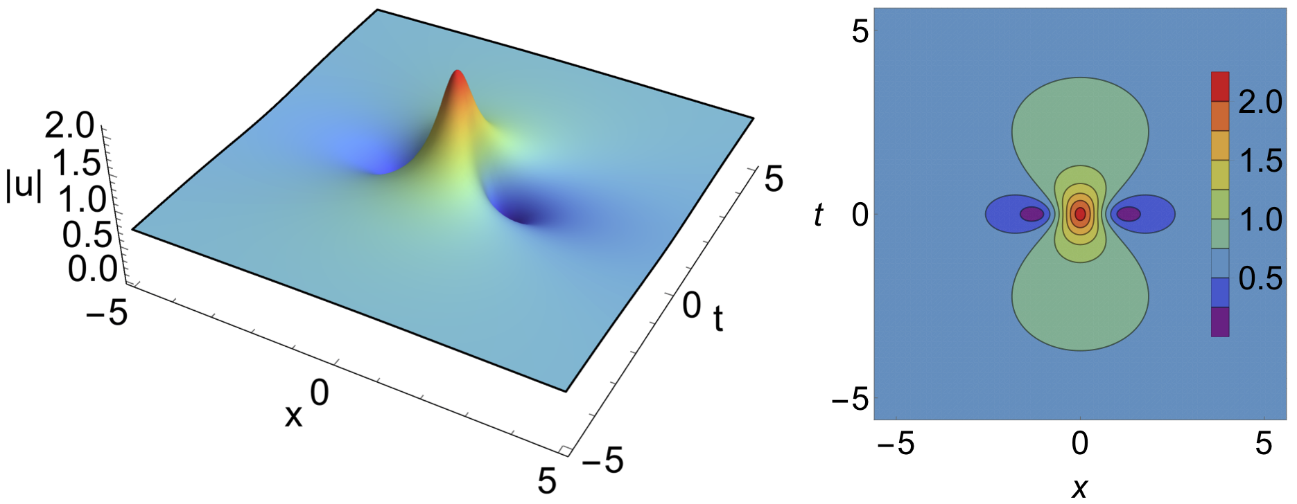
Figure 1: Intensity and contour plot of the Peregrine breather solution (2) for $\alpha=0.7$.

Now, we consider the following form of the Benjamin-Ono (BO) equation:

$$u_{tt}+2\beta u_{x}^{2}+2\beta uu_{xx}+\gamma u_{xxxx}=0,$$ (3)

where $\beta$ and $\gamma$ are arbitrary nonlinearity and dispersion coefficients, respectively. The Benjamin-Ono equation describes one-dimensional internal waves in deep water tbb ; hon . It is mathematically a famous nonlinear partial integrodifferential equation possessing integrability and solvable by inverse scattering transform as well as possess Bäcklund transformation, Painlevé singularity analysis and also admitting $N$-soliton solutions asf ; kmc ; kmt ; rij and have infinite conserved quantities apart from special rational and periodic solutions ana ; jsat . Its various other solutions, including nonlocal symmetries yli and rogue wave solutions wli , are available in the literature. Our aim of the present work is to explore various physically significant solutions such as rogue waves, breathers, and solitons with a newly developed method and study their control mechanism along with the interaction, bending, fusion, and fission of nonlinear waves especially solitons.

Now by using a bilinearizing transformation, we write the BO equation into a compact bilinear form and then solve it by introducing a polynomial test function of the required order. For this purpose, by making use of the following transformation

$$u(x,t)=u_{0}+\dfrac{6\gamma}{\beta}(ln\,f)_{xx},$$ (4)

where $u_{0}$ is an arbitrary background while $f(x,t)$ is a arbitrary function to be determined, the BO equation (3) is transformed into the following Bilinear form:

$$(D_{t}^{2}+2u_{0}\beta D_{x}^{2}+\gamma D_{x}^{4})f\cdot f=0.$$ (5)

Here $D$ represents the standard Hirota differential operator wli ; NLD2017BO ; Hirota-book and it can be defined as

$$D_{x}^{a}D_{y}^{b}f\cdot g=\left(\dfrac{\partial}{\partial x}-\dfrac{\partial}{\partial x^{\prime}}\right)^{a}\left(\dfrac{\partial}{\partial y}-\dfrac{\partial}{\partial y^{\prime}}\right)^{b}f(x,y,t)\cdot g(x^{\prime},y^{\prime},t^{\prime})|_{(x,y,t)=(x^{\prime},y^{\prime},t^{\prime})}.$$

In recent years, localized structures such as rogue waves, breathers, and lump solutions arising in various nonlinear models attract more concentration and they become interesting both in mathematical and physical perspective due to their occurrence in diversified areas like plasmas, optics, Bose-Einstein condensate, and financial systems rogue-book ; nak ; PRX-rogue .

The present work is organized as follows. In Sec. 2, the first and second-order rogue wave solutions are constructed using the Hirota bilinear form and polynomial test functions ylm . In Sec. 3, the generalized breather solutions of different wave structures are obtained by using the three-wave method wta2 along with their evolution dynamics. And conclusions are provided in the final section.

2 Rogue Waves

In this section, we construct the first and second-order rogue wave solutions using the bilinear form (5) and appropriate polynomial test functions and investigate their evolution with respect to different control parameters.

2.1 Rogue wave solution of order-one

To extract the rogue wave solution of order-one, we choose the form of $f(x,t)$ as ylm :

$$f(x,t)=k_{0}+(\alpha_{1}x+\beta_{1}t)^{2}+(\alpha_{2}x+\beta_{2}t)^{2}.$$ (6)

Substituting the above form of $f$ (6) into bilinear equation (5) and collecting the coefficients of different powers of $\{x^{i}y^{j},~{}i,j=0,1,2\}$, we get the following set of equations:

$$\text{ Coefficient of }x^{2} :(-4u_{0}\alpha_{1}^{4}\beta-8u_{0}\alpha_{1}^{2}\alpha_{2}^{2}\beta-4u_{0}\alpha_{2}^{4}\beta-2\alpha_{1}^{2}+\beta_{1}^{2}+2\alpha_{2}^{2}\beta_{1}^{2}-8\alpha_{1}\alpha_{2}\beta_{1}\beta_{2}$$

$$+2\alpha_{1}^{2}\beta_{2}^{2}-2\alpha_{2}^{2}\beta_{2}^{2})=0,$$ (7a)

$$\text{ Coefficient of }t^{2} :(-4u_{0}\alpha_{1}^{2}\beta\beta_{1}^{2}+4u_{0}\alpha_{2}^{2}\beta\beta_{1}-2\beta_{1}^{4}-16u_{0}\alpha_{1}\alpha_{2}\beta\beta_{1}\beta_{2}+4u_{0}\alpha_{1}^{2}\beta\beta_{2}^{2}$$

$$-4u_{0}\alpha_{2}^{2}\beta\beta_{2}^{2}-4\beta_{1}^{2}\beta_{2}^{2}-2\beta_{2}^{4})=0,$$ (7b)

$$\text{ Coefficient of }tx :(-8u_{0}\alpha_{1}^{3}\beta\beta_{1}-8u_{0}\alpha_{1}\alpha_{2}^{2}\beta\beta_{1}-4\alpha_{1}\beta_{1}^{3}-8u_{0}\alpha_{1}^{2}\alpha_{2}\beta\beta_{2}-8u_{0}\alpha_{2}^{3}\beta\beta_{2}$$

$$-4\alpha_{2}\beta_{1}^{2}\beta_{2}-4\alpha_{1}\beta_{1}\beta_{2}^{2}-4\alpha_{2}\beta_{2}^{3})=0,$$ (7c)

Constants $$:(4k_{0}u_{0}\alpha_{1}^{2}\beta+4k_{0}u_{0}\alpha_{2}^{2}\beta+2k_{0}\beta_{1}^{2}+2k_{0}\beta_{2}^{2}+12\alpha_{1}^{4}\gamma+24\alpha_{1}^{2}\alpha_{2}^{2}\gamma+12\alpha_{2}^{4}\gamma)=0.$$ (7d)

Solving the above system of equations (7a)-(7d), we obtain the following relations among the parameters resulting to the first-order rogue wave solution as

$$u_{0}\beta>0,\quad\beta_{1} =\pm\sqrt{2u_{0}\beta}\alpha_{2},\quad\beta_{2}=\mp\sqrt{2u_{0}\beta}\alpha_{1},\quad k_{0}=\dfrac{-3(\alpha_{1}^{2}+\alpha_{2})^{2}\gamma}{2u_{0}\beta}.$$ (8)

From Eqs. (8) and (6), we get the explicit form of $f$ as

$$f(x,t)=\left(\alpha_{1}x+\sqrt{2u_{0}\beta}\,\alpha_{2}t\right)^{2}+\left(\alpha_{2}x-\sqrt{2u_{0}\beta}\,\alpha_{1}t\right)^{2}-\dfrac{3(\alpha_{1}^{2}+\alpha_{2}^{2})\gamma}{2u_{0}\beta}.$$ (9)

Thus, we can obtain the first-order rouge wave solution from (4) and (9) as

$$u(x,t)=u_{0}+\dfrac{24u_{0}\gamma(-2u_{0}x^{2}\beta+4t^{2}u_{0}^{2}\beta^{2}-3\gamma)}{(2u_{0}x^{2}\beta+4t^{2}u_{0}^{2}\beta^{2}-3\gamma)^{2}},$$ (10)

under the constraint condition $u_{0}\beta>0$. The above solution carries three arbitrary parameters $u_{0},~{}\beta$, and $\gamma$. It is of natural interest to understand importance and roles of these arbitrary parameters in defining the dynamics of the rogue wave solution (10). We can obtain two types of rogue waves, namely bright and dark, by tuning these parameters as shown in Fig. 2 by retaining the necessary condition $u_{0}\beta>0$. We mainly obtain bright single peak doubly localized excitation with the choice $u_{0}=-1.05$, $\beta=-1.01$, and $\gamma=1.05$. On the other hand, a dark type first-order rogue wave structure is depicted for another choice $u_{0}=1.05$, $\beta=0.3$, and $\gamma=-0.05$.

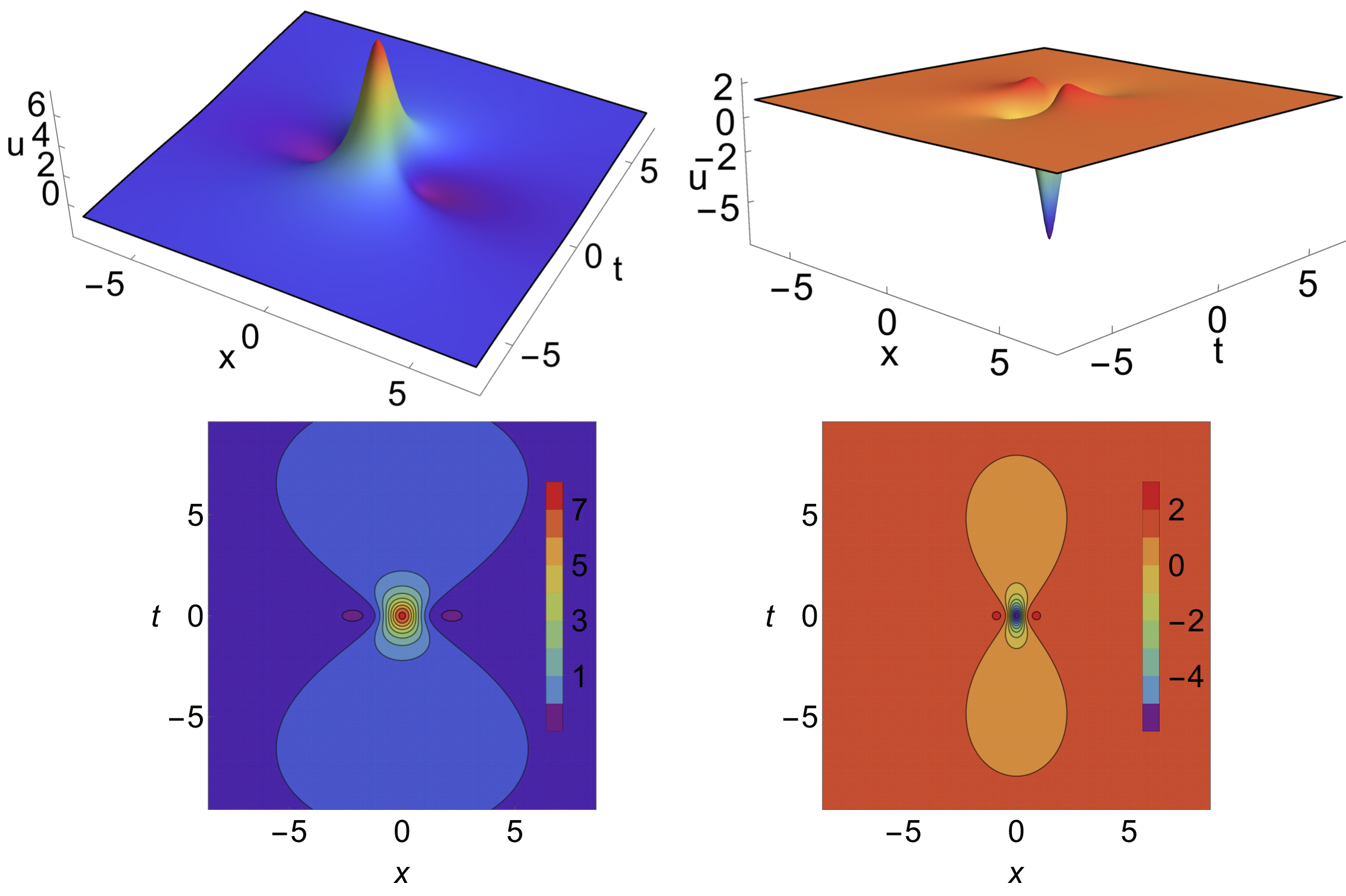
Figure 2: Bright (left panel) and dark (right panel) type first-order rogue waves through solution (10). The bottom panel shows the corresponding contour plots.

For a much clear inference of the arbitrary parameters, we have demonstrated their role graphically for the bright rogue wave with three different sets of values in Fig. 3. Our analysis shows that the increase in the magnitude of $\beta$ decreases the width of the rogue waves, while the $\gamma$ parameter is altering its width in direct proportion with an appreciable change in their tail and without affecting the amplitude. However, the parameter $u_{0}$ is much simpler, increasing the amplitude of the rogue wave and a shift from its constant background. Importantly, there occurs an appreciable change in the significant wave height (amplitude) of the amplitude. Similar effects can also be observed in the dark rogue wave case, which is shown in Fig. 4, where the depth/darkness, background, width, and tail of the dark rogue waves are controlled by tuning $\beta$, $\gamma$, and $u_{0}$ parameters.

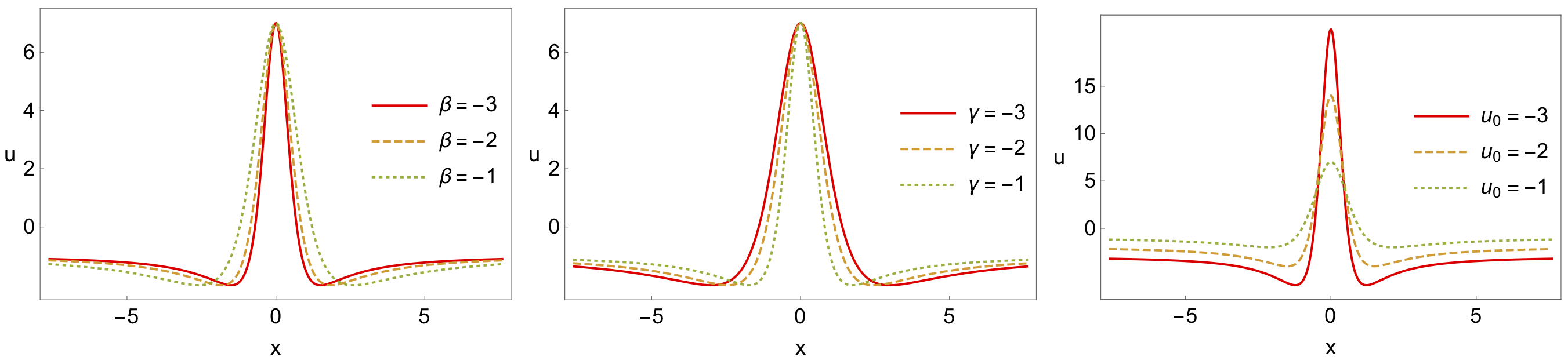
Figure 3: Impact of $\beta$, $\gamma$ and $u_{0}$ parameters in the first-order bright rogue wave (10) for fixed values of other parameters.

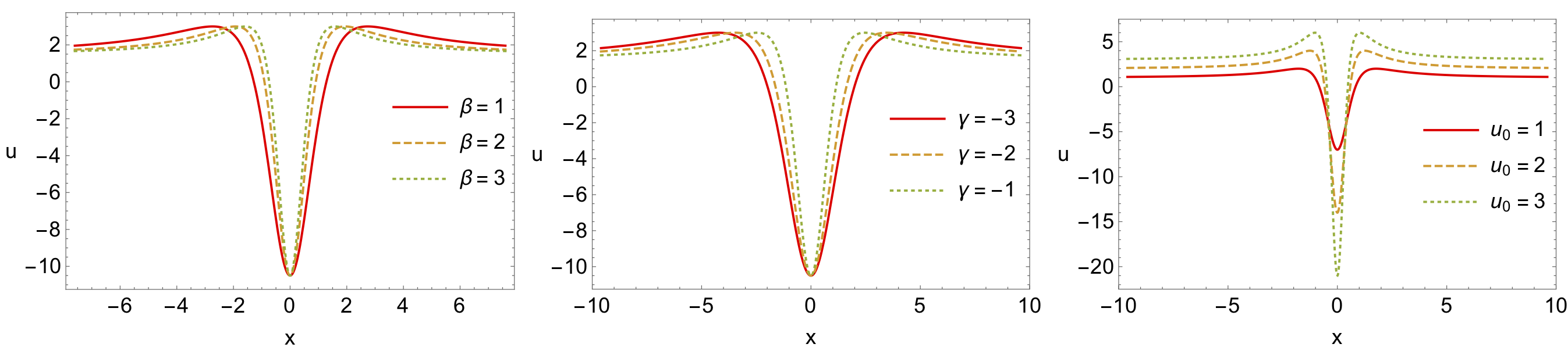
Figure 4: Impact of $\beta$, $\gamma$ and $u_{0}$ parameters in the first-order dark rogue wave (10) for fixed values of other parameters.

2.2 Rogue wave solution of order-two

The next natural step is to construct and look for higher-order rogue waves and their dynamical behaviour in the present BO equation. Here we construct a simplest higher-order rogue wave, which is the rogue wave of order two. For this purpose, we have adopted the following polynomial test function ylm :

$$f(x,t)=\beta_{1}+\left(\beta_{2}x^{2}+\beta_{3}t^{2}\right)^{3}+\beta_{4}x^{4}+\beta_{5}x^{2}t^{2}+\beta_{6}t^{4}+\beta_{7}x^{2}+\beta_{8}t^{2},$$ (11)

where $\beta_{j}(j=1,2,\ldots,8)$ are parameters of second-order rogue wave solution, will be determined later. Substituting (11) into the bilinear form (5) and equating to zero the coefficients of $\{x^{m}y^{n},\quad m,n=0,1,2,3,4,5,6,7,8\}$, we obtained the following algebraic nonlinear system of equations:

$$\text{Coefficient of }x^{10}: -12u_{0}\beta\beta_{2}^{6}+6\beta_{2}^{5}\beta_{3}=0,$$ (12a)

$$\text{Coefficient of }t^{2}x^{8}: -36u_{0}\beta\beta_{2}^{5}\beta_{3}+18\beta_{2}^{4}\beta_{3}^{2}=0,$$ (12b)

$$\text{Coefficient of }t^{4}x^{6}: -24u_{0}\beta\beta_{2}^{4}\beta_{3}^{2}+12\beta_{2}^{3}+\beta_{3}^{3}=0,$$ (12c)

$$\text{Coefficient of }t^{6}x^{4}: 24u_{0}\beta\beta_{2}^{3}\beta_{3}^{3}-12\beta_{2}^{2}\beta_{3}^{4}=0,$$ (12d)

$$\text{Coefficient of }t^{8}x^{2}: 36u_{0}\beta\beta_{2}^{2}\beta_{3}^{4}-18\beta_{2}\beta_{3}^{5}=0,$$ (12e)

$$\text{Coefficient of }t^{10}: 12u_{0}\beta\beta_{2}\beta_{3}^{5}-6\beta_{3}^{6}=0,$$ (12f)

$$\text{Coefficient of }x^{8}: -12u_{0}\beta\beta_{2}^{3}\beta_{4}+6\beta_{2}^{2}\beta_{3}\beta_{4}+2\beta_{2}^{3}\beta_{5}+180\beta_{2}^{6}\gamma=0,$$ (12g)

$$\text{Coefficient of }t^{2}x^{6}: -48u_{0}\beta\beta 2^{2}\beta_{3}\beta_{4}+36\beta_{2}\beta_{3}^{2}\beta_{4}+16u_{0}\beta\beta_{2}^{2}\beta_{5}-12\beta_{2}^{2}\beta_{3}\beta_{5}+12\beta_{2}^{3}\beta_{6}$$ (12h)

$$+144\beta_{2}^{5}\beta_{3}\gamma=0,$$

$$\text{Coefficient of }t^{4}x^{4}: -12u_{0}\beta\beta_{2}\beta_{3}^{2}\beta_{4}+30\beta_{3}^{3}\beta_{4}-12u_{0}\beta\beta_{2}^{2}\beta_{3}\beta_{5}-6\beta_{2}\beta_{3}^{2}\beta_{5}+60u_{0}\beta\beta_{2}^{3}\beta_{6}-6\beta_{2}^{2}\beta_{3}\beta_{6}$$ (12i)

$$-72\beta_{2}^{4}\beta_{3}^{2}\gamma=0,$$

$$\text{Coefficient of }t^{6}x^{2}: 24u_{0}\beta\beta_{3}^{3}\beta_{4}-24u_{0}\beta\beta_{2}\beta_{3}^{2}\beta_{5}+8\beta_{3}^{3}\beta_{5}+72u_{0}\beta\beta_{2}^{2}\beta_{3}\beta_{6}-24\beta_{2}\beta_{3}^{2}\beta_{6}+144\beta_{2}^{3}\gamma=0,$$ (12j)

$$\text{Coefficient of }t^{8}: 4u_{0}\beta\beta_{3}^{3}\beta_{5}+12u_{0}\beta\beta_{2}\beta_{3}^{2}\beta_{6}-6\beta_{3}^{3}\beta_{6}+180\beta_{2}^{2}\beta_{3}^{4}\gamma=0,$$ (12k)

$$\text{Coefficient of }x^{6}: -8u_{0}\beta\beta_{4}^{2}+2\beta_{4}\beta_{5}+16u_{0}\beta\beta_{2}^{3}\beta_{7}+6\beta_{2}^{2}\beta_{3}\beta_{7}+2\beta_{2}^{3}\beta_{8}+48\beta_{2}^{3}\beta_{4}\gamma=0,$$ (12l)

$$\text{Coefficient of }t^{2}x^{4}: -4u_{0}\beta\beta_{4}\beta_{5}-2\beta_{5}^{2}+12\beta_{4}\beta_{6}-12u_{0}\beta\beta_{2}^{2}\beta_{3}\beta_{7}+36\beta_{2}\beta_{3}^{2}\beta_{7}+60u_{0}\beta\beta_{2}^{3}\beta_{8}$$ (12m)

$$-12\beta_{2}^{2}\beta_{3}\beta_{8}+432\beta_{2}^{2}\beta_{3}\beta_{4}\gamma-240\beta_{2}^{3}\beta_{5}\gamma=0,$$

$$\text{Coefficient of }t^{4}x^{2}: -4u_{0}\beta beta_{5}^{2}+24u_{0}\beta\beta_{4}\beta_{6}-2\beta_{5}\beta_{6}-24u_{0}\beta\beta_{2}\beta_{3}^{2}\beta_{7}+30\beta_{3}^{3}\beta_{7}+72u_{0}\beta\beta_{2}^{2}\beta_{3}\beta_{8}$$ (12n)

$$-6\beta_{2}\beta_{3}^{2}\beta_{8}-72\beta_{2}\beta_{3}^{2}\beta_{4}\gamma-72\beta_{2}^{2}\beta 3\beta_{5}\gamma+360\beta_{2}^{2}\beta_{6}\gamma=0,$$

$$\text{Coefficient of }t^{6}: 4u_{0}\beta\beta_{5}\beta_{6}-4\beta_{6}^{2}+4u_{0}\beta\beta_{3}^{3}\beta_{7}+12u_{0}\beta\beta_{2}\beta_{3}^{2}\beta_{8}+8\beta_{3}^{3}\beta_{8}+24\beta_{3}^{3}\beta_{4}\gamma+72\beta_{2}\beta_{3}^{2}\beta_{5}\gamma$$ (12o)

$$+72\beta_{2}^{2}\beta_{3}\beta_{6}\gamma=0,$$

$$\text{Coefficient of }x^{4}: 60u_{0}\beta\beta_{1}\beta_{2}^{3}+6\beta_{1}\beta_{2}^{2}\beta_{3}-4u_{0}\beta\beta_{4}\beta_{7}+2\beta_{5}\beta_{7}+2\beta_{4}\beta_{8}+72\beta_{4}^{2}\gamma-240\beta_{2}^{3}\beta_{7}\gamma=0,$$ (12p)

$$\text{Coefficient of }x^{2}: 24u_{0}\beta\beta_{1}\beta_{4}+2\beta_{1}\beta_{5}-4u_{0}\beta\beta_{7}^{2}+2\beta_{7}\beta_{8}+360\beta_{1}\beta_{2}^{3}\gamma-24\beta_{4}\beta_{7}\gamma=0,$$ (12q)

$$\text{Coefficient of }t^{2}x^{2}: 72u_{0}\beta\beta_{1}\beta_{2}^{2}\beta_{3}+36\beta_{1}\beta_{2}\beta_{3}^{2}-8u_{0}\beta\beta_{5}\beta_{7}+12\beta_{6}\beta_{7}+24u_{0}\beta\beta_{4}\beta_{8}-4\beta_{5}\beta_{8}-24\beta_{4}\beta_{5}\gamma$$ (12r)

$$-72\beta_{2}^{2}\beta_{3}\beta_{7}\gamma+360\beta_{2}^{3}\beta_{8}\gamma=0,$$

$$\text{Coefficient of }t^{4}: 12u_{0}\beta\beta_{1}\beta_{2}\beta_{3}^{2}+30\beta_{1}\beta_{3}^{3}+4u_{0}\beta\beta_{6}\beta_{7}+4u_{0}\beta\beta_{5}\beta_{8}-2\beta_{6}\beta_{8}+12\beta_{5}^{2}\gamma+24\beta_{4}\beta_{6}\gamma$$ (12s)

$$+72\beta_{2}\beta_{3}^{2}\beta_{7}\gamma+72\beta_{2}^{2}\beta_{3}\beta_{8}\gamma=0,$$

$$\text{Coefficient of }t^{2}: 4u_{0}\beta\beta_{1}\beta_{5}+12\beta_{1}\beta_{6}+4u_{0}\beta\beta_{7}\beta_{8}-2\beta_{8}^{2}+72\beta_{1}\beta_{2}^{2}\beta_{3}\gamma+24\beta_{5}\beta_{7}\gamma+24\beta_{4}\beta_{8}\gamma=0,$$ (12t)

$$\text{Constants}: 4u_{0}\beta\beta_{1}\beta_{7}+2\beta_{1}\beta_{8}+24\beta_{1}\beta_{4}\gamma+12\beta_{7}^{2}\gamma=0.$$ (12u)

By solving the above system of equations, we get the following set of relations among the parameters:

$$\beta_{1} =\dfrac{-1875\beta_{3}^{3}\gamma^{3}}{64u_{0}^{6}\beta^{6}};\quad\beta_{2}=\dfrac{\beta_{3}}{2u_{0}\beta};\quad\beta_{4}=\dfrac{-25\beta_{3}^{3}\gamma}{16u_{0}^{4}\beta^{4}};\quad\beta_{5}=\dfrac{-45\beta_{3}^{3}\gamma}{4u_{0}^{3}\beta^{3}};$$ (13)

$$\beta_{6} =\dfrac{-17\beta_{3}^{3}\gamma}{4u_{0}^{2}\beta^{2}};\quad\beta_{7}=\dfrac{-125\beta_{3}^{3}\gamma^{2}}{32u_{0}^{5}\beta^{5}};\quad\beta_{8}=\dfrac{475\beta_{3}^{3}\gamma^{2}}{16u_{0}^{4}\beta^{4}}.$$

From Eqs. (4), (11) and (13), we obtained the two-rogue wave solution of Benjamin-Ono equation (3) as follows:

$$u(x,t)=u_{0}+\dfrac{6\gamma}{\beta}\left(\dfrac{F_{1}}{F_{2}^{2}}\right),$$ (14a)

where

$$F_{1} = 4u_{0}\beta(4608t^{8}u_{0}^{9}x^{2}\beta^{9}+3072t^{10}u_{0}^{10}\beta^{10}+531250u_{0}x^{2}\beta\gamma^{4}+234375\gamma^{5}$$ (14b)

$$+62500u_{0}^{2}\beta^{2}\gamma^{3}(-2x^{4}+7t^{2}\gamma)+768t^{4}u_{0}^{7}x^{2}\beta^{7}(-x^{4}+14t^{2}\gamma)-768t^{6}u_{0}^{8}\beta^{8}(-2x^{4}+47t^{2}\gamma)$$

$$-2000u_{0}^{3}x^{2}\beta^{3}\gamma^{2}(7x^{4}+510t^{2}\gamma)+400u_{0}^{4}\beta^{4}\gamma(3x^{8}+210t^{2}x^{4}\gamma-1850t^{4}\gamma^{2})$$

$$-96u_{0}^{5}x^{2}\beta^{5}(x^{8}+20t^{2}x^{4}\gamma-1250t^{4}\gamma^{2})+64t^{2}u_{0}^{6}\beta^{6}(-9x^{8}+90t^{2}x^{4}\gamma+2830t^{4}\gamma^{2})),$$

$$F_{2} = 96t^{4}u_{0}^{5}x^{2}\beta^{5}+64t^{6}u_{0}^{6}\beta^{6}-250u_{0}x^{2}\beta\gamma^{2}-1875\gamma^{3}+8u_{0}^{3}x^{2}\beta^{3}(x^{4}-90t^{2}\gamma)$$ (14c)

$$-100u_{0}^{2}\beta^{2}\gamma(x^{4}-19t^{2}\gamma)+16t^{2}u_{0}^{4}\beta^{4}(3x^{4}-17t^{2}\gamma).$$

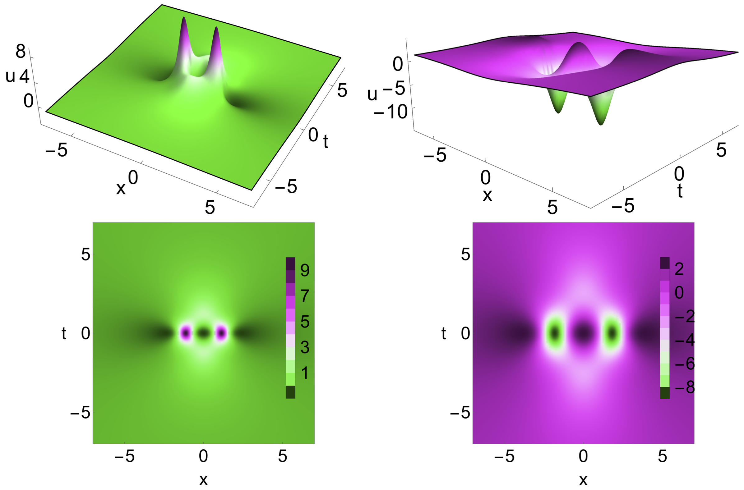
Figure 5: Bright (left panel) and dark (right panel) type second-order rogue waves through solution (14). The bottom panel shows the corresponding contour plot. The parameter choice for bright rogue wave is $u_{0}=-1.05$, $\beta=-1.01$, $\beta_{3}=1.1$ and $\gamma=0.5$, while that of dark rogue wave is $u_{0}=1.5$, $\beta=0.41$, $\beta_{3}=1.1$ and $\gamma=-0.75$.

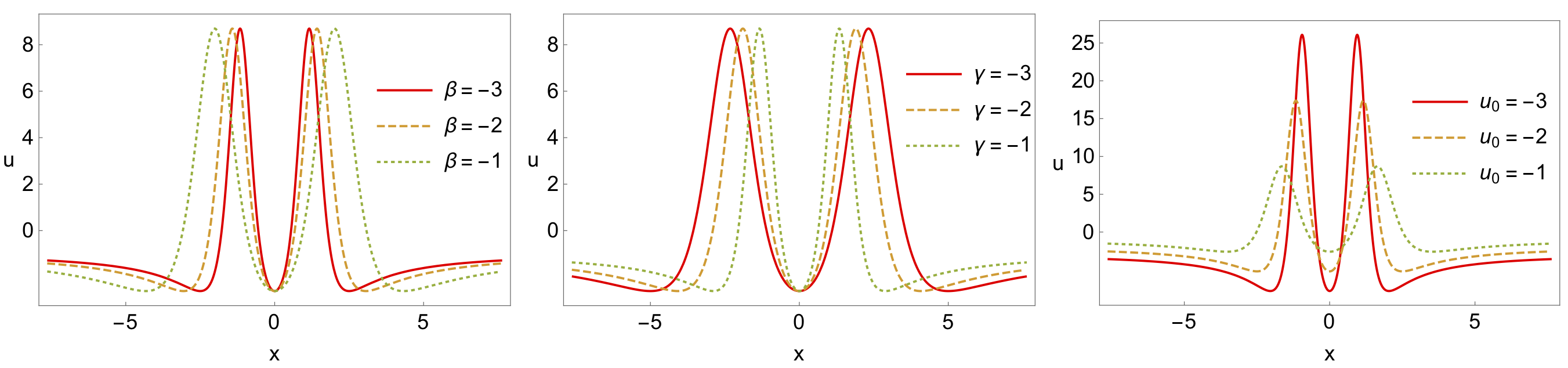
Figure 6: Manipulation of the second-order bright rogue wave (10) by controlling the parameters $\beta$, $\gamma$ and $u_{0}$.

Our categorical analysis on the above second-order rogue wave solution reveals that there exist two types of rogue waves, namely bright and dark rogue waves, as appeared in the case of first-order rogue wave solutions. For completeness, we have shown such a bright and dark type second-order rogue wave structures in Fig. 5 and the respective choices of parameters are given in the caption. Further, the impact of arbitrary parameters $\beta$, $\gamma$, and $u_{0}$ gives additional freedom to manipulate the amplitude or depth, width, background and tail of the second-order rogue waves too. Such effects of these parameters in the second-order bright rogue wave are demonstrated in Fig. 6. Similarly, these effects can also be observed in the dark rogue wave, which is not given here by considering the length of the article.

3 Generalized Breathers

As given in the introduction, the second part of this work is to investigate the dynamics of generalized breathers of the Benjamin-Ono equation (3), which we carry out in this section. For this purpose, we first obtain the breather solutions of BO model (3) by adopting a generalized three-wave test function suggested in Ref. ygu , which is also referred to as the three-wave method. Here the following form of homoclinic breather (two-wave) ansatz xby is generalized to obtain the homoclinic breathers as well as travelling wave solutions:

$$f(x,t)=m_{1}e^{(p_{1}x+k_{1}t)}+m_{2}\cos(q_{1}x+a_{1}t)+m_{1}e^{-(p_{1}x+k_{1}t)},$$ (15)

were $m_{1},m_{2},p_{1},k_{1},q_{1},a_{1}$ are arbitrary constants. The above one is a combination of two waves, a periodic wave $\cos(q_{1}x+a_{1}t)$ and a hyperbolic wave $\cosh(p_{1}x+k_{1}t)$, which gives rise to homoclinic breathers. For more generalized breather wave solutions, we consider a combination of three waves as initial test function as given below ygu .

$$f(x,t)=b_{1}e^{(px+kt)}+b_{2}\cos(qx-at)+b_{3}e^{-(px+kt)}+b_{4}\cosh(mx+ct),$$ (16)

where $b_{1},b_{2},b_{3},b_{4},p,k,q,a,m$ and $c$ are unknown parameters to be determined for generalized breathers. Here the choice $b_{4}=0$ in (16) correspond to the homoclinic breathers of the two-wave interaction method (15). Thus, we construct homoclinic breather solutions without loss of generality, which exhibits different nonlinear wave structures ranging from bright/dark solitons, breathers, etc. by following the above three-wave interaction method. It is also clear that the number of arbitrary parameters in the three-wave method is higher than two-wave homoclinic breathers.

Further, one can also use the following form of the test function, as suggested in Ref. wta3 for a KdV type system,

$$f(x,t)=b_{1}\cosh(\Xi_{1})+b_{2}\cos(\Xi_{2})+b_{3}\cosh(\Xi_{3}),$$ (17)

where $\Xi_{i}=k_{i}(n_{i}x+r_{i}y+s_{i}t+\alpha_{i}),~{}i=1,2,3,$ and $n_{i},r_{i},s_{i},\alpha_{i}$ are the arbitrary parameters. This newly introduced test function is similar to the three-wave solution test function. In a similar way, a generalized N-wave method can also be used to find various solutions of nonlinear integrable/non-integrable equations, which is beyond the scope of the current work and can be investigated separately to look for other types of possible nonlinear wave entities.

3.1 Breather Solution using Three-Wave method

Considering the three-wave test function (16) and collecting the coefficients of $e^{i(px+kt)}$, $\cos(qx-at)$, $\sin(qx-at)$, $\cosh(mx+ct)$, $\sinh(mx+ct),(i=-1,0,1)$, we get the following system of algebraic equations from Eq. (5):

$$(8b_{1}b_{3}k^{2}+16b_{1}b_{3}p^{2}u_{0}\beta+32b_{1}b_{3}p^{4}\gamma)+(-2a^{2}b_{2}^{2}-4b_{2}^{2}q^{2}u_{0}\beta+8b_{2}^{2}q^{4}\gamma)$$

$$+(2b_{4}c^{2}+4b_{4}^{2}m^{2}u_{0}\beta+8b_{4}^{2}m^{4}\gamma)=0,$$ (18a)

$$-2a^{2}b_{2}b_{3}+2b_{2}b_{3}k^{2}+4b_{2}b_{3}p^{2}u_{0}\beta-4b_{2}b_{3}q^{2}u_{0}\beta+2b_{2}b_{3}p^{4}\gamma-12b_{2}b_{3}p^{2}q^{2}\gamma+2b_{2}b_{3}q^{4}\gamma=0,$$ (18b)

$$-2a^{2}b_{1}b_{2}+2b_{1}b_{2}k^{2}+4b_{1}b_{2}p^{2}u_{0}\beta-4b_{1}b_{2}q^{2}u_{0}\beta+2b_{1}b_{2}p^{4}\gamma-12b_{1}b_{2}p^{2}q^{2}\gamma+2b_{1}b_{2}q^{4}\gamma=0,$$ (18c)

$$2b_{1}b_{4}c^{2}+2b_{1}b_{4}k^{2}+4b_{1}b_{4}m^{2}u_{0}\beta+4b_{1}b_{4}p^{2}u_{0}\beta)+(2b_{1}b_{4}m^{4}\gamma+12b_{1}b_{4}m^{2}b^{2}\gamma+2b_{1}b_{4}b^{4}\gamma=0,$$ (18d)

$$2b_{3}b_{4}c^{2}+2b_{3}b_{4}k^{2}+4b_{3}b_{4}m^{2}u_{0}\beta+4b_{3}b_{4}u_{0}\beta+2b_{3}b_{4}m^{4}\gamma+12b_{3}b_{4}m^{2}p^{2}\gamma+2b_{3}b_{4}p^{4}\gamma=0,$$ (18e)

$$-2a^{2}b_{2}b_{4}+2b_{2}b_{4}c^{2}+4b_{2}b_{4}m^{2}u_{0}\beta-4b_{2}b_{4}q^{2}u_{0}\beta+2b_{2}b_{4}m^{4}\gamma-12b_{2}b_{4}m^{2}q^{2}\gamma+2b_{2}b_{4}q^{4}\gamma=0,$$ (18f)

$$4ab_{1}b_{2}k-8b_{1}b_{2}pqu_{0}\beta-8b_{1}b_{2}p^{3}q\gamma+8b_{1}b_{2}pq^{3}\gamma=0,$$ (18g)

$$-4ab_{2}b_{3}k+8b_{2}b_{3}pqu_{0}\beta+8b_{2}b_{3}p^{3}q\gamma-8b_{2}b_{3}pq^{3}\gamma=0,$$ (18h)

$$-4b_{1}b_{4}ck-8b_{1}b_{4}mpu_{0}\beta-8b_{1}b_{4}m^{3}p\gamma-8b_{1}b_{4}mp^{3}\gamma=0,$$ (18i)

$$4b_{3}b_{4}ck+8b_{3}b_{4}mpu_{0}\beta+8b_{3}b_{4}m^{3}p\gamma+8b_{3}b_{4}mp^{3}\gamma=0,$$ (18j)

$$4ab_{2}b_{4}c-8b_{2}b_{4}mqu_{0}\beta-8b_{2}b_{4}m^{3}q\gamma+8b_{2}b_{4}mq^{3}\gamma=0.$$ (18k)

After solving the above nonlinear algebraic system of equations, different classes of solutions can be obtained for the arbitrary parameters which we discuss one by one in the following part.

Case 1: When $b_{1}=b_{3}=b_{4}=0$ and $b_{2}\neq 0$, Eqs. (18) give $a=\sqrt{2(2q^{4}\gamma-q^{2}u_{0}\beta)}$ with $b_{2}$ as an arbitrary free parameter. This results into the following form of $f$:

$$f=b_{2}\cos\left(qx-\sqrt{2(2q^{4}\gamma-q^{2}u_{0}\beta)}t\right).$$ (19)

Thus we get a singular solution of the Benjamin Ono equation (5) as

$$u(x,t)=u_{0}-\dfrac{6\gamma}{\beta}\left(q^{2}\sec^{2}(qx-t\sqrt{2(2q^{4}\gamma-q^{2}u_{0}\beta)}\right).$$ (20)

The above solution always result into unbounded singular form without much advantages or applications. So, here we do not discuss any further details of the obtained solution (20).

Case 2: When $b_{1}=b_{3}=0$ and $b_{2},b_{4}\neq 0$, the explicit form of $f$ is obtained from Eqs. (18) as

$$f=b_{2}\cos\left[\left(\frac{\sqrt{(u_{0}\beta+2m^{2}\gamma)}}{\sqrt{2\gamma}}\right)\left(\sqrt{3}x-2m\sqrt{\gamma}t\right)\right]+\frac{2\sqrt{-2b_{2}^{2}(u_{0}\beta+2m^{2}\gamma}}{\sqrt{u_{0}\beta+8m^{2}\gamma}}$$

$$\times\cosh\left[mx-\sqrt{\dfrac{3}{4\gamma}}\left({u_{0}\beta+4m^{2}\gamma}\right)t\right],$$ (21a)

where $$b_{4}=2\sqrt{\dfrac{-2b_{2}^{2}(u_{0}\beta+2m^{2}\gamma)}{u_{0}\beta+8m^{2}\gamma}} q=\sqrt{\dfrac{3(u_{0}\beta+2m^{2}\gamma)}{2\gamma}} c=-\sqrt{\dfrac{3}{4\gamma}}{(u_{0}\beta+4m^{2}\gamma)} a=\sqrt{2m^{2}(u_{0}\beta+2m^{2}\gamma)} u_{0},~{}\beta,~{}\gamma,~{}b_{2} m f$$, , , and while the other parameters ( and ) are arbitrary. From the above and Eqn. (4), we can obtain the exact solution as below.

$$u(x,t)=u_{0}+\dfrac{6\gamma}{\beta}(ln\,f)_{xx}.$$ (21b)

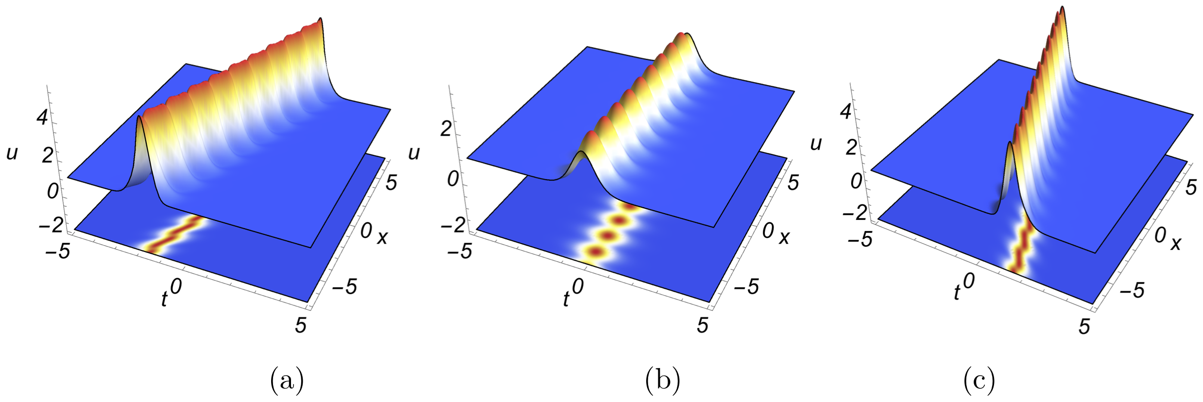
Figure 7: Breathing soliton with periodical oscillation in amplitude and space for (a) $m=0.75$, (b) $m=0.0$ and (c) $m=-0.75$. Other arbitrary parameters are fixed as $u_{0}=1$, $\gamma=0.5$, $\beta=1.50$, and $b_{2}=1.0$.

This clearly shows that the contribution from both ‘cos’ and ‘cosh’ parts giving rise to the breathing nature of soliton, which may be of either bright (zero background) or anti-dark (non-zero background) solitons for an appropriate choice. Further, the breathing (period of) oscillations can be controlled in addition to the manipulation of breather velocity (direction of propagation), amplitude and width by tuning the available arbitrary parameters. To be specific, the $u_{0}$ parameter controls the background energy and amplitude of the breather, while $\gamma$ influences the amplitude and velocity. However, the parameter $\beta$ varies the width of the soliton breather in addition to its velocity changes. For illustrative purposes, we have given a bright soliton breather on a constant non-zero energy/amplitude (anti-dark soliton breathers) in Fig. 7 travelling with positive, zero, and negative velocity having different amplitudes.

Another striking feature in the above obtained solution (21), which is nothing but the interaction of two stable solitons and it occurs when there exist the background amplitude/intensity. This includes the collision between (i) two single-hump (anti-dark) solitons, (ii) single-well (dark) and single-hump (anti-dark) solitons, (iii) rational type and dark solitons, and (iv) bound state formation among two anti-dark solitons by choosing the appropriate choices of parameters as shown in Fig. 8 for elucidation. Here we have depicted the elastic (amplitude or shape preserving) collision of two non-equal amplitude anti-dark solitons (Fig. 8a), while such elastic collision can also be possible among two equal amplitude solitons. We can easily witness that though the solitons are interacting elastically, they undergo a phase-shift after collision (clearly visible in contour plots). Soliton bound states are nothing but two solitons travelling with same velocity (velocity resonance) exhibit periodic attraction and repulsion of their central position during propagation. This can also happen in higher-dimensional solitons as well as among solitons undergoing an inelastic collisions . For more detailed investigation on soliton collisions and bound states please refer soli-int1 ; soli-int2 ; soli-int3 ; bound1 ; bound2 ; bound3 and references therein.

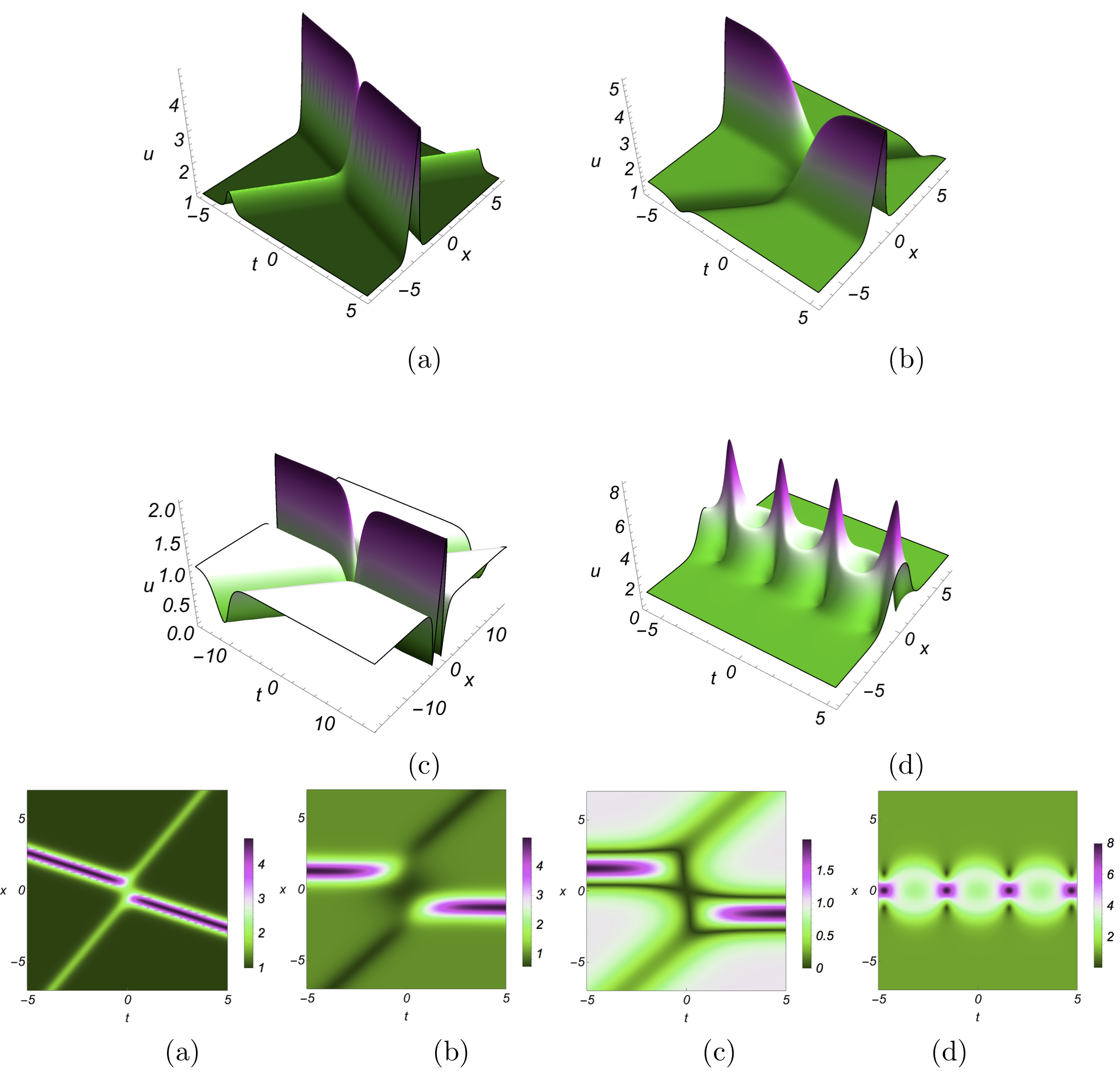
Figure 8: Elastic interaction between (a) among two single-hump (anti-dark) solitons, (b) anti-dark and dark solitons, (c) dark and rational solitons, and (d) bound state of two anti-dark solitons through (21). Bottom panel shows the contour plot of these interacting solitons. The parameter choices are (a) $u_{0}=1.0$, $\beta=-2.5$, $\gamma=0.5$, $b_{2}=1.0$, $p=-1.0$, & $m=0.5$, (b) $u_{0}=1.0$, $\beta=-1.15$, $\gamma=0.5$, $b_{2}=1.0$, $p=-1.0$, & $m=0.5$, (c) $u_{0}=1.0$, $\beta=-0.95$, $\gamma=0.5$, $b_{2}=1.0$, $p=-1.0$, & $m=0.5$, and (d) $u_{0}=1.0$, $\beta=1.0$, $\gamma=-0.75$, $b_{2}=1.0$, $p=-1.0$, & $m=0.0$.

Case 3: For the choice $b_{2}=b_{4}=0$ and $b_{1},b_{3}\neq 0$, Eqs. (18) reduces to an explicit form of $f$ as

$$f=b_{1}e^{(px-\sqrt{2(-p^{2}u_{0}\beta-2p^{4}\gamma)}t)}+b_{3}e^{-(px-\sqrt{2(-p^{2}u_{0}\beta-2p^{4}\gamma}t)},$$ (22)

along with $k=-\sqrt{-2p^{2}(u_{0}\beta+2p^{2}\gamma)}$. Further, by setting $b_{1}=b_{3}>0$, the function $f(x,t)$ becomes

$$f(x,t)=2b_{1}\cosh\left(px-\sqrt{-2p^{2}(u_{0}\beta+2p^{2}\gamma}t\right).$$ (23a)

Hence the solution of BO equation (3) is obtained as the following stable soliton:

$$u(x,t)=u_{0}+\dfrac{6\gamma}{\beta}p^{2}\mbox{sech}^{2}\left(px-t\sqrt{-2p^{2}(u_{0}\beta+2p^{2}\gamma})\right).$$ (23b)

On the other hand, when $b_{1}=d_{1},b_{3}=-d_{1}$ with $d_{1}>0$ the function $f(x,t)$ reduces to

$$f(x,t)=2d_{1}\sinh\left(px-\sqrt{-2p^{2}(u_{0}\beta+2p^{2}\gamma}t\right).$$ (24a)

Now, the corresponding solution of BO equation (3) can be derived as a hyperbolic solution given below.

$$u(x,t)=u_{0}-\dfrac{6\gamma}{\beta}p^{2}\mbox{cosech}^{2}\left(px-t\sqrt{-2p^{2}(u_{0}\beta+2p^{2}\gamma})\right).$$ (24b)

From the above solutions, namely Eqs. (23b) and (24b), one can understand that they correspond to bright/dark soliton and unbounded structures, respectively. Though the singular solutions are of no further interest, solitons found multifaceted applications due to their stable propagation with various localized profiles of salient features. In the present case, the solution (23b) is further divided into two categories: (i) bright solitons (localized stable waves appearing on a zero-background $u_{0}=0$) and (ii) dark/gray/anti-dark solitons (stable localized waves arising on a non-zero background $u_{0}\neq 0$). In bright soliton case ($u_{0}=0$), an additional restriction on the parameters ($\gamma<0$) also arise, which overcomes/removes the singular structures. Such bright solitons travel with velocity $\sqrt{-4p^{4}\gamma}$ and possess an amplitude of $\dfrac{6\gamma}{\beta}p^{2}$. The second case ($u_{0}\neq 0$), we obtain various profile structures ranging from anti-dark, dark, gray and rational type solitons for different choices of other parameters provided they satisfy $u_{0}\beta+2p^{2}\gamma<0$. These nonlinear wave structures admit an amplitude $u_{0}+\dfrac{6\gamma}{\beta}p^{2}$ and propagates with velocity $\sqrt{-2p^{2}(u_{0}\beta+2p^{2}\gamma)}$. Among these, the anti-dark soliton resembles with standard bright solitons, but it appear on the constant background and with different velocity. On the other hand, the dark solitons can also be divided into two sub-categories called dark and gray solitons, where the former localized waves have zero lowest amplitude (depth of the well structure), while in the latter they admit non-zero well depth. Additionally, we have identified bright and dark type rational solitons by controlling the arbitrary parameter $p$. Here the dark rational solitons can be viewed as a double-well (W-shaped) dark solitons, while the bright rational soliton is nothing but a localized hump/peak with side-band minima on either side of localization. By preserving these relations and tuning the available parameters, one can manipulate their width and amplitude along with propagation direction appropriately. For completeness and better understanding, we have shown such bright, anti-dark, dark, and gray solitons in addition to bright and dark rational solitons in Fig. 9.

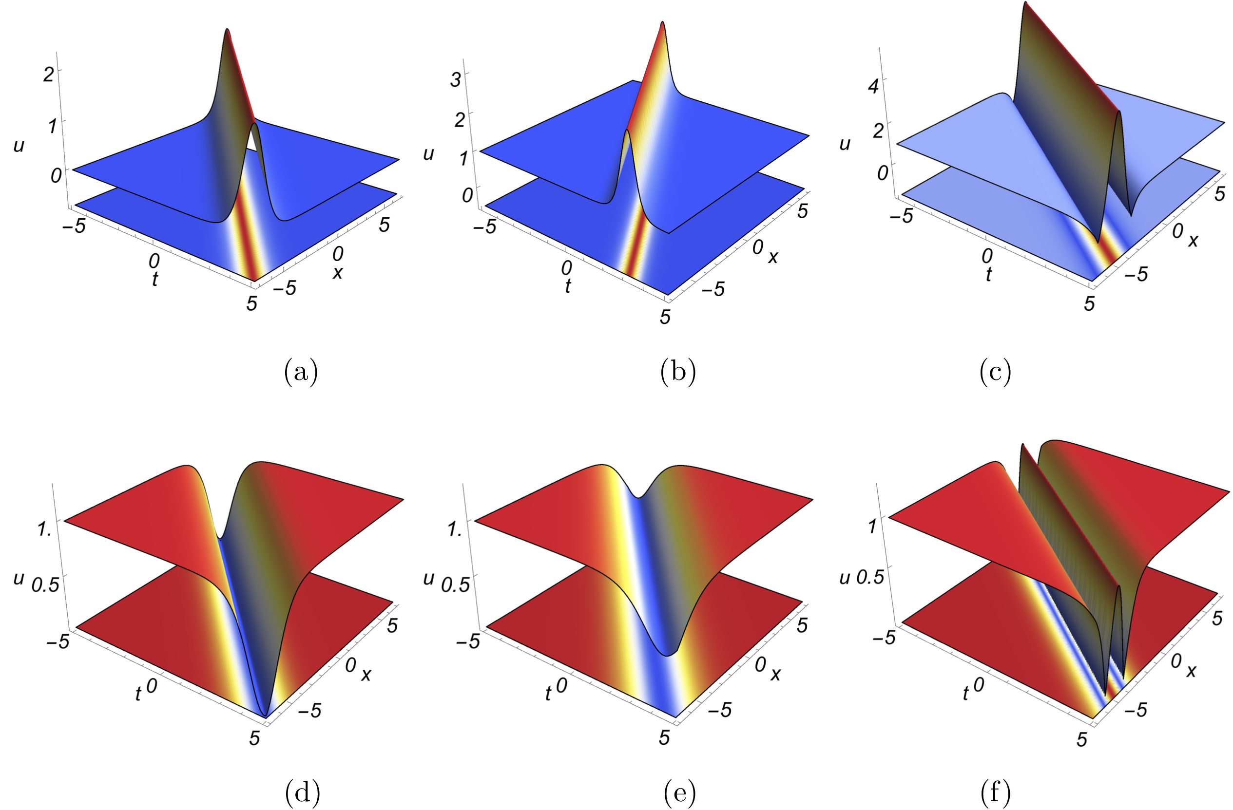
Figure 9: Propagation of (a) bright soliton, (b) anti-dark soliton (bright soliton on a constant background $u_{0}\neq 0$), (c) rational soliton, (d) single-well dark soliton, (e) single-well gray solitons, and W-shaped (double well) dark soliton of BO equation through Eq. (23b). The parameters are chosen as (a) $u_{0}=0$, $\gamma=-0.5$, $\beta=-1.5$, $d_{1}=1.0$, & $p=-1.0$, (b) $u_{0}=1.0$, $\gamma=-0.5$, $\beta=-1.5$, $d_{1}=1.0$, & $p=-1.0$, (c) $u_{0}=1.0$, $\gamma=-0.5$, $\beta=0.5$, $d_{1}=1.5$, & $p=-1.0$, (d) $u_{0}=1.0$, $\gamma=0.5$, $\beta=-1.5$, $d_{1}=1.0$, & $p=-0.7$, (e) $u_{0}=1.0$, $\gamma=0.5$, $\beta=-1.5$, $d_{1}=1.0$, & $p=-0.5$, and (f) $u_{0}=1.0$, $\gamma=0.5$, $\beta=-1.5$, $d_{1}=1.0$, & $p=-1.0$.

Case 4: When $b_{1}=0$ and $b_{2},b_{3},b_{4}\neq 0$, we can obtain the explicit form of $f$ from the set of equations (18) as below.

$$f(x,t)=b_{2}\cos(qx-at)+b_{3}e^{-(px+kt)}+b_{4}\cosh(mx+ct),$$ (25a)

where the parameters $$m,~{}p,~{}k,~{}a q$$ and take the following form:

$$m=\dfrac{1}{2\sqrt{\gamma}}\sqrt{-u_{0}\beta-\Delta},\quad p=\sqrt{\dfrac{3}{4\gamma}}\sqrt{-u_{0}\beta+\Delta},$$ (25b)

$$k=\frac{-\sqrt{3}\Delta}{4c\gamma}\sqrt{-(u_{0}\beta+\Delta)}\sqrt{-(u_{0}\beta-\Delta)},\qquad\quad$$ (25c)

$$a=\dfrac{1}{4c\gamma}{(u_{0}\beta-\Delta)\sqrt{-(u_{0}\beta+\Delta)^{2}}},\qquad$$ (25d)

$$q=\dfrac{1}{2\sqrt{\gamma}}\sqrt{u_{0}\beta+\Delta},\quad\mbox{with}\quad\Delta=\sqrt{u_{0}^{2}\beta^{2}-4c^{2}\gamma}.$$ (25e)

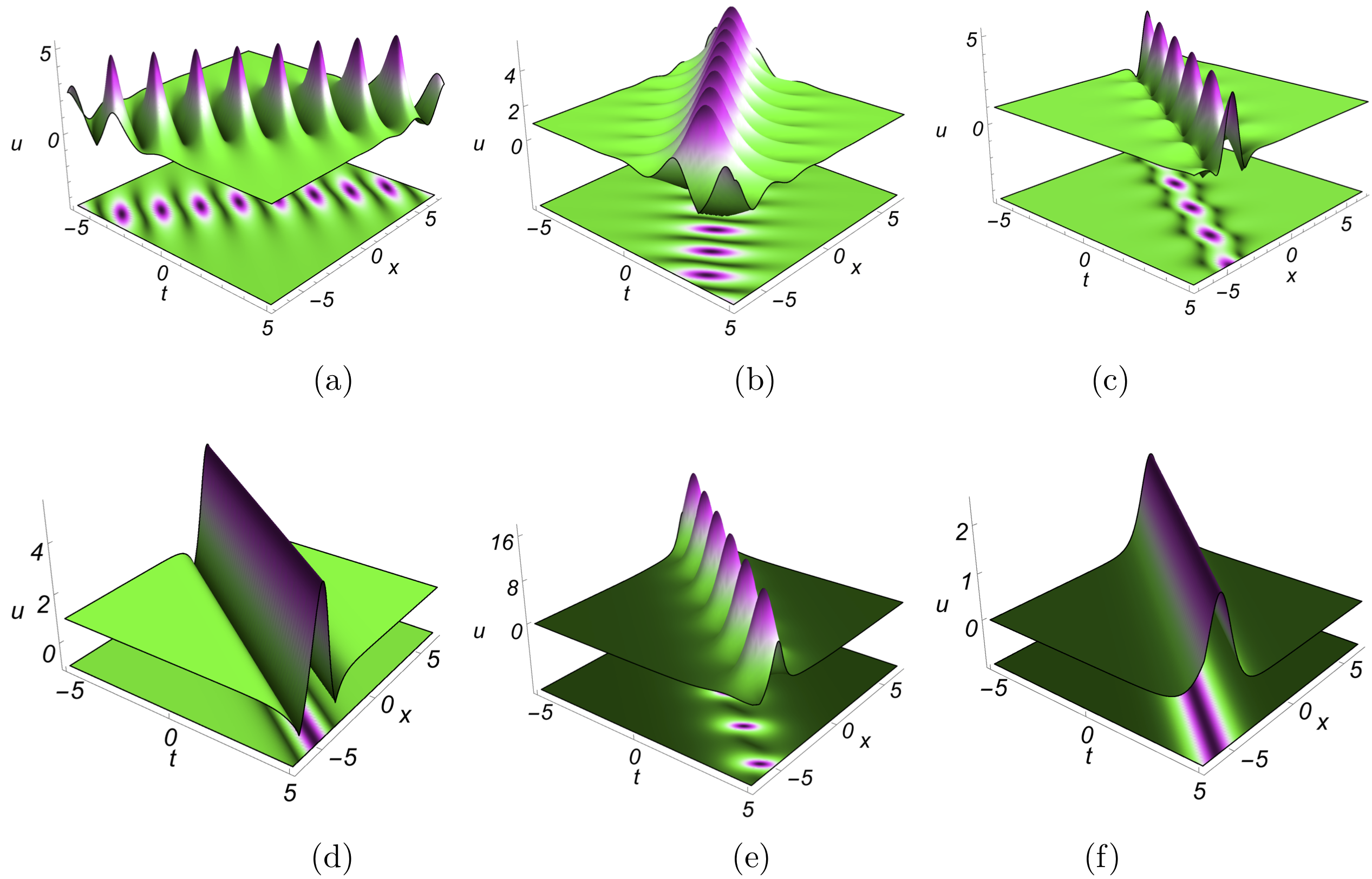
Figure 10: Propagation of (a-d) soliton breathers appearing on a constant background, and (e) breathing and (f) stable bright solitons on zero-background on through (25). The parameter choices are (a) $u_{0}=1$, $\beta=-1.5$, $\gamma=-0.5$, $b_{2}=1.0$, $b_{3}=0.5$, $b_{4}=1.5$, & $c=-1.0$, (b) $u_{0}=1$, $\beta=-1.5$, $\gamma=-0.5$, $b_{2}=-1.0$, $b_{3}=-0.5$, $b_{4}=1.5$, & $c=1.0$, (c) $u_{0}=1$, $\beta=1.5$, $\gamma=-0.75$, $b_{2}=1.0$, $b_{3}=0.5$, $b_{4}=1.5$, & $c=1.0$, (d) $u_{0}=1$, $\beta=0.5$, $\gamma=-0.5$, $b_{2}=0.5$, $b_{3}=0.0$, $b_{4}=0.5$, & $c=1.0$, (e) $u_{0}=0.0$, $\beta=1.0$, $\gamma=-0.5$, $b_{2}=0.5$, $b_{3}=-0.5$, $b_{4}=-1.5$, & $c=1.0$, and (f) $u_{0}=0.0$, $\beta=1.0$, $\gamma=-0.5$, $b_{2}=0.5$, $b_{3}=0.0$, $b_{4}=-1.5$, & $c=1.0$.

In the above solution (25), $u_{0}$, $\beta$, $\gamma$, $c$, $b_{2}$, $b_{3}$, and $b_{4}$ are the seven arbitrary parameters through which we can manipulate the resultant nonlinear wave pattern of soliton breather. Compared to the previous solutions, the above solution reveals exciting patterns of soliton breather explaining various phenomena. It starts from the breathing of solitons with periodic oscillations in its amplitude as well as stable rational soliton on non-zero background $u_{0}\neq 0$ and stable/standard bright soliton without any background ($u_{0}=0$). Further, we have also identified solitons with single or double hump/well structure undergoing fusion and fission processes in addition to their bending characteristics. Such type of soliton breather is shown in Fig. 10, while the bending, fission, and fusion nature of solitons are demonstrated in Figs. 11–13 with an appropriate choice of arbitrary parameters. Here one can also control the amplitude, period of oscillations/breathing, width, and velocity of solitons/breathers by tuning the arbitrary parameters.

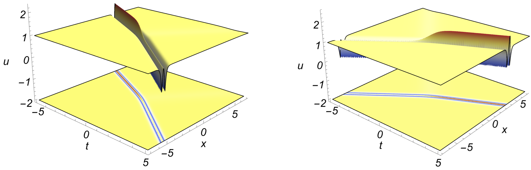
Figure 11: Bending of W-shaped dark soliton with decrease/increase in the intensity due to increased/decreased width of the soliton given by Eqn. (25) for $c=-0.5$ (left panel) and $c=0.5$ (right panel) with other arbitrary parameters as $u_{0}=1$, $\beta=-1.5$, $\gamma=0.25$, $b_{2}=1.0$, $b_{3}=0.5$, and $b_{4}=1.5$.

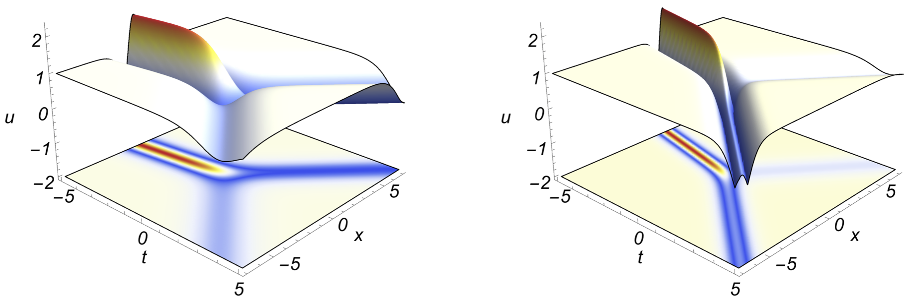
Figure 12: Fission of a W-shaped dark soliton into two single well solitons (for $u_{0}=1$, $\beta=-1.5$, $\gamma=0.5$, $b_{2}=1.0$, $b_{3}=0.5$, $b_{4}=1.5$, and $c=1.0$) and a single well soliton and double well gray solitons (for $u_{0}=1$, $\beta=-1.5$, $\gamma=0.25$, $b_{2}=1.0$, $b_{3}=0.5$, $b_{4}=1.5$, and $c=-1.0$) through Eqn. (25).

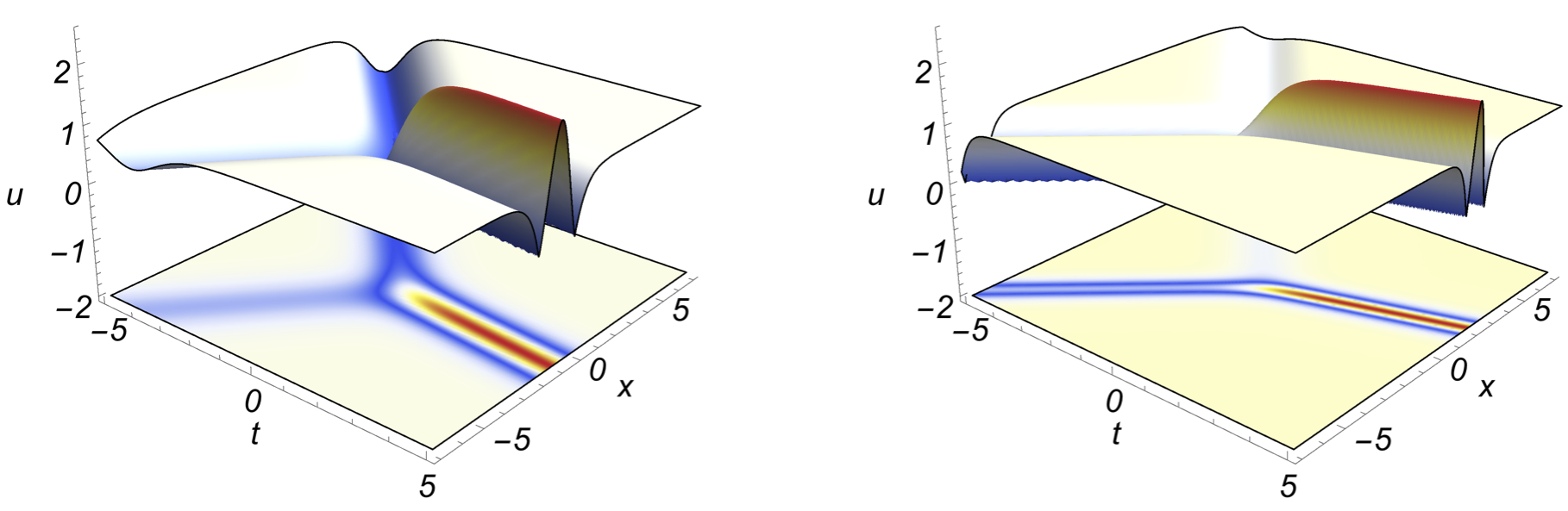
Figure 13: Fusion of two single well solitons (for $u_{0}=1$, $\beta=-1.5$, $\gamma=0.5$, $b_{2}=1.0$, $b_{3}=0.5$, $b_{4}=1.5$, and $c=1.0$) and a single well soliton with double well soliton (for $u_{0}=1$, $\beta=-1.5$, $\gamma=0.25$, $b_{2}=1.0$, $b_{3}=0.5$, $b_{4}=1.5$, and $c=1.0$) to form amplified W-shaped dark soliton through Eqn. (25).

As a future study, the present three-wave interaction (test function) method can be further extended/generalized to arbitrary $N$-wave interaction, which shall reveal several interesting features/dynamics including the interaction among breathers as well as the collision of solitons with breathers. Considering the computational complexity and length of the manuscript, we have not studied here, but it will be worth to explore.

4 Conclusion

We have considered the Benjamin-Ono equation and constructed various localized wave solutions starting from the rogue waves to breathers and solitons by employing polynomial test functions and three-wave method with the aid of bilinear form. Through the obtained solutions, we are able to control and manipulate the constructed localized waves with the available arbitrary parameters to realize their multifaceted nature such as tailoring of their amplitude, width, velocity, and tail/valley of both bright and dark type first as well as second-order rogue waves, developing bright/anti-dark, dark/gray, and rational solitons, the interaction of dark, anti-dark, and rational solitons, exploring the formation of bound states, fusion, fission and bending properties of solitons with clear graphical demonstrations. The reported results will be helpful for a complete understanding of the dynamics of the considered Benjamin-Ono model, and further, the analysis can be extended to other related nonlinear models.

References

- (1) M. Lakshmanan, S. Rajasekar, Nonlinear Dynamics: Integrability, Chaos and Patterns (Springer, Berlin, 2003).
- (2) R. Sakthivel, C. Chun, J. Lee, New travelling wave solutions of Burgers equation with finite transport memory, Zeitschrift für Naturforschung A 65 (2010) 633-640.
- (3) J. Yang, Nonlinear Waves in Integrable and Nonintegrable Systems (SIAM, Philadelphia, 2010).
- (4) B. Guo, X-F. Pang, Y-F. Wang, N. Liu, Solitons (De Gruyter, Berlin, 2018).
- (5) H. Kim, R. Sakthivel, A. Debbouche, D. F.M. Torres, Traveling wave solutions of some important Wick-type fractional stochastic nonlinear partial differential equations, Chaos Solitons Fractals, 131 (2020) 109542.
- (6) M. Onorato, S. Resitori, F. Baronio, Rogue and Shock Waves in Nonlinear Dispersive Media (Springer, New York, 2016).
- (7) N. Akhmediev, A. Ankiewicz, M. Tak, Waves that appear from nowhere and disappear without a trace, Phys Lett A 373 (2009) 675–678.
- (8) G. Dematteis, T. Grafke, M. Onorato, E. V. Eijnden, Experimental Evidence of Hydrodynamic Instantons: The Universal Route to Rogue Waves, Phys Rev X 9 (2019) 041057.
- (9) Z. Y. Yan, Financial rogue waves, Commun Theor Phys. 54 (2010) 947–949.
- (10) W.M. Moslem, P.K. Shukla, B. Eliasson, Surface plasma rogue waves, Euro Phys Lett 96 (2011) 25002.
- (11) V. B. Efimov, A.N. Ganshin, G.V. Kolmakov, P.V.E. McClintock, L.P. Mezhov-Deglin, Rogue waves in supefluid helium, Eur Phys J Special Topics 185 (2010) 181-193 .
- (12) Y.V. Bludov, V.V. Konotop, N. Akhmediev, Matter rogue waves, Phys Rev A 80 (2009) 033610.
- (13) D.R. Solli, C. Ropers, P. Koonath, B. Jalali, Optical rogue waves, Nature 450 (2007) 1054–1057.
- (14) B. Guo, L. Tian, Z. Yan, L. Ling, Y-F. Wang, Rogue waves: Mathematical theory and applications in physics (De Gruyter, Berlin, 2017).
- (15) C. Kharif, E. Pelinovsky, A. Slunyaev, Rogue waves in the ocean: Advances in Geophysical and Environmental Mechanics and Mathematics (Springer, Berlin, 2009).
- (16) N. Akhmediev, J.M. Dudley, D.R. Solli, and S.K. Turitsyn, Recent progress in investigating optical rogue waves, J Opt 15 (2013) 060201.
- (17) J. H. Choi, H. Kim, R. Sakthivel, Periodic and solitary wave solutions of some important physical models with variable coefficients, Waves Random Complex Media (2019) https://doi.org/10.1080/17455030.2019.1633029.
- (18) H. Kim, R. Sakthivel, Travelling wave solutions for time-delayed nonlinear evolution equations, Appl Math Lett 23 (2010) 527-532.
- (19) Y. Kivshar, G. P. Agrawal, Optical solitons: From fibers to photonic crystals (Academic Press, San Diego, 2003).
- (20) A. Calini, C.M. Schober, M. Strawn, Linear instability of the Peregrine breather: Numerical and analytical investigations, Appl Num Math 141 (2019) 36–43.
- (21) D. H. Peregrine, Water waves, nonlinear Schrödinger equations and their solutions, J Austral Math Soc Ser B 25 (1983) 16–43.
- (22) T. B. Benjamin, Internal waves of permanent form in fluids of great depth, J Fluid Mech 29 (1967) 559-572.
- (23) H. Ono, Algebraic Solitary Waves in Stratified Fluids, J Phys Soc Japan 39 (1975) 1082-1091.
- (24) A. S. Fokas, M. J. Ablowitz, The inverse scattering transform for the Benjamin-Ono equation, Stud Appl Math 68 (1983) 1-10.
- (25) K. M. Case, The N-Soliton solution of the Benjamin-Ono equation, Proc Natl Acad Sci USA 75 (1978) 3562-3563.
- (26) K. M. Tamizhmani, A. Ramani, B. Grammaticos, Singularity confinement analysis of integro-differential equation of Benjamin-Ono equation, J Phys A: Math Gen 30 (1997) 1017-1022.
- (27) R. I. Joseph, Multisoliton like solutions of Benjamin-Ono equation, J Math Phys 181 (1977) 2251.
- (28) A. Nakamura, Bäcklund transform and conservation laws of the Benjamin-Ono equation, J Phys Soc Japan 47 (1979) 4.
- (29) J. Satsuma, Y. Ishimori, Periodic wave and rational soliton solutions of the Benjamin-Ono equation, J Phys Soc Japan 46 (1979) 2.
- (30) Y. Li, H. Hu, Nonlocal symmetries and interaction solutions of the Benjamin-Ono equation, Appl Math Lett 75 (2018) 18-23.
- (31) W. Liu, High-order rogue waves of the Benjamin Ono equation and the nonlocal nonlinear Schrödinger equation, Mod Phys Lett B 31 (2017) 1750269.
- (32) W. Tan, Z. Dai, Spatiotemporal dynamics of lump solution to the (1+1)-dimensional Benjamin-Ono equation, Nonlinear Dyn 89 (2017) 2723–2728.
- (33) R. Hirota, The Direct Method in Soliton Theory (Cambridge University Press, Cambridge, 2003).
- (34) Y. Guo, The new exact solutions of the Fifth-Order Sawada-Kotera equation using three wave method, Appl Math Lett 94 (2019) 232-237.
- (35) X-B. Yang, S-F. Tian, C-Y. Qin, T-T. Zhang, Characteristics of the breather, rogue waves and solitary waves in a generalized (2+1)-dimensional Boussinesq equation, Euro Phys Lett 115 (2016) 10002.
- (36) W. Tan, W. Zhang, J. Zhang, Evolutionary behavior of breathers and interaction solutions with M-solitons for (2+1)-dimensional KdV system, Appl Math Lett 101 (2020) 106063.
- (37) Y-L. Ma, B-Q. Li, Analytic rogue wave solutions for a generalized fourth-order Boussinesq equation in fluid mechanics, Math Meth Appl Sci 42 (2019) 39-48.
- (38) W. Tan, Evolution of breathers and interaction between high order lumps solutions and N-solitons for breaking soliton system, Phys Lett A 383 (2019) 125907.
- (39) T. Kanna and M. Lakshmanan. Exact soliton solutions, shape changing collisions, and partially coherent solitons in coupled nonlinear Schrödinger equations, Phys Rev Lett 86 (2001) 5043.
- (40) A. Gkogkou and B. Prinari, Soliton interactions in certain square matrix nonlinear Schrödinger systems, Eur Phys J Plus 135 (2020) 609.
- (41) J. Chai, B. Tian, X.Y. Wu, and L. Liu, Fusion and fission phenomena for the soliton interactions in a plasma, Eur Phys J Plus 132 (2017) 60.
- (42) K. Sakkaravarthi and T. Kanna. Dynamics of bright soliton bound states in (2+1)-dimensional multicomponent long wave-short wave system, Eur Phys J Special Topics 222 (2013) 641-653.
- (43) S. Li and G. Biondini, Soliton interactions and degenerate soliton complexes for the focusing nonlinear Schrödinger equation with nonzero background, Eur Phys J Plus 133 (2018) 400.
- (44) E.N.N.N. Aboringong and A.M. Dikandé, Soliton lattices originating from excitons interacting with high-intensity fields in finite molecular crystals, Eur Phys J Plus 134 (2019) 609.