Noise-Induced Randomization in
Regression Discontinuity Designs

Abstract

Regression discontinuity designs assess causal effects in settings where treatment is determined by whether an observed running variable crosses a pre-specified threshold. Here we propose a new approach to identification, estimation, and inference in regression discontinuity designs that uses knowledge about exogenous noise (e.g., measurement error) in the running variable. In our strategy, we weight treated and control units to balance a latent variable of which the running variable is a noisy measure. Our approach is explicitly randomization-based and complements standard formal analyses that appeal to continuity arguments while ignoring the stochastic nature of the assignment mechanism.

Keywords: causal inference, randomization-based inference, bias-aware inference, latent variable model, empirical Bayes

1 Introduction

Regression discontinuity designs are a popular approach to causal inference that rely on known, discontinuous treatment assignment mechanisms to identify causal effects (Hahn, Todd, and van der Klaauw, 2001; Imbens and Lemieux, 2008; Thistlethwaite and Campbell, 1960). More specifically, we assume the existence of a running variable $Z_{i}\in\mathbb{R}$ such that unit $i$ gets assigned treatment $W_{i}\in\left\{0,\,1\right\}$ whenever the running variable exceeds a cutoff $c\in\mathbb{R}$, i.e., $W_{i}=1\left(\left\{Z_{i}\geq c\right\}\right)$. For example, in an educational setting where admission to a program hinges on a test score exceeding some cutoff, we could evaluate the effect of the program on marginal admits by comparing outcomes for students whose test scores fell right above and below the cutoff.

Explanations and qualitative justifications of identification in regression discontinuity designs often appeal to implicit, local randomization: There are many factors outside the control of decision-makers that determine the running variable $Z_{i}$ such that if some unit barely clears the eligibility cutoff for the intervention then the same unit could also plausibly have failed to clear the cutoff with a different realization of these chance factors (Lee and Lemieux, 2010). This is sometimes illustrated by reference to sampling error or other errors in measurement that cause units to have a measured running variable just above or just below the threshold. For example, in our educational setting, there may be a group of marginal students who might barely pass or fail the test due to unpredictable variation in their test score, thus resulting in an effectively exogenous treatment assignment rule. Likewise, medical assays frequently involve a degree of random measurement error, whether because of sampling techniques or other sources of random variation (Bor et al., 2014).

Most formal and practical approaches to identification, estimation, and inference for treatment effects in regression discontinuity designs, however, do not use exogenous noise in the running variable to drive inference. Instead, following Hahn, Todd, and van der Klaauw (2001), the dominant approach relies on a continuity argument. As in Imbens and Lemieux (2008), we assume potential outcomes $\left\{Y_{i}(0),\,Y_{i}(1)\right\}$ such that $Y_{i}=Y_{i}(W_{i})$. Then, we can identify a weighted treatment effect $\tau_{c}=\mathbb{E}\left[Y_{i}(1)-Y_{i}(0)\,\big{|}\,Z_{i}=c\right]$ via

$$\tau_{c}=\lim_{z\downarrow c}\mathbb{E}\left[Y\,\big{|}\,Z=z\right]-\lim_{z\uparrow c}\mathbb{E}\left[Y\,\big{|}\,Z=z\right],$$ (1)

provided that the conditional response functions $\mu_{(w)}(z)=\mathbb{E}\left[Y(w)\,\big{|}\,Z=z\right]$ are continuous. As we further explain in Section 1.2, if we are willing to posit quantitative smoothness bounds on $\mu_{(w)}(z)$, then we can use this continuity-based argument to derive confidence intervals for $\tau_{c}$ with well understood asymptotics.

Despite its appeal and simple formulation, the continuity-based approach to regression discontinuity inference does not satisfy the criteria for rigorous design-based causal inference as outlined by Rubin (2008). According to the design-based paradigm, even in observational studies, a treatment effect estimator should be justifiable based on randomness in the treatment assignment mechanism alone; the leading example of this paradigm is the analysis of randomized controlled trials following Neyman (1923) and Rubin (1974). In contrast, the formal guarantees provided by the continuity-based regression discontinuity analysis often take smoothness of $\mu_{(w)}(z)$ as a primitive. While continuous measurement error in (or “imprecise control” of) the running variable by units implies continuity of the conditional expectation function (Lee, 2008), this result is not used in estimation and inference and, as we show, only makes limited use of the identifying power of measurement error, perhaps most notably for discrete running variables.

Here we propose a new approach to regression discontinuity inference—one that goes back to the above qualitative argument used to justify regression discontinuity designs and directly exploits noise in the running variable $Z_{i}$ for inference. Formally, we assume the existence of a latent variable $U_{i}$, and that any variation in the running variable $Z_{i}$ around $U_{i}$ is exogenous. For example, again revisiting our educational setting, we can take $U_{i}$ to be a measure of the student’s true ability; then the test score $Z_{i}$ is a noisy measurement of $U_{i}$ with well-documented psychometric properties. Likewise, in a medical setting, the running variable $Z_{i}$ may be a measurement of an underlying condition $U_{i}$ (e.g., CD4 counts); such diagnostic measurements often have well-studied test-retest reliability. In both cases, it is plausible that the measurements $Z_{i}$ are independent of relevant potential outcomes conditional on the underlying quantity $U_{i}$.

Our main result is that, if the measurement error in $Z_{i}$ has a known distribution and the measurement error is conditionally independent of potential outcomes, then we can estimate weighted treatment effects that correspond to the effects of realistic changes to the existing treatment assignment rule. We then propose a practical approach to estimation and inference in regression discontinuity designs that builds on this result. Unlike in the classical regression discontinuity design, our inference is—at least in the case of bounded outcomes—driven entirely by noise-induced randomization, that is, by random treatment assignment induced by noise in $Z_{i}$. Our approach is conceptually appealing, offers clarity, and transparency on the key assumption (noise-induced randomization) driving inference, and furthermore allows for inference of policy-relevant estimands beyond (1).

We emphasize that, while this noise-induced randomization approach applies to many settings of interest, it does not apply to all regression discontinuity designs. Some running variables are not readily interpretable as having measurement error or other exogenous noise; or we may not have a-priori information on the distribution of this noise. For example, numerous studies have used geographic boundaries as discontinuities (Keele and Titiunik, 2014; Rischard, Branson, Miratrix, and Bornn, 2021), but it would be questionable to model the location of a household in space as having meaningful measurement error; perhaps, following Ganong and Jäger (2018), it may be more plausible to argue that the location of the boundary itself is random. Likewise, analyses of close elections—a central example of regression discontinuity designs in political science and economics (Caughey and Sekhon, 2011; Lee, 2008)—may not allow for a natural noise model for $Z_{i}$ that would arise from, e.g., noisy counting of the number of ballots cast for each candidate, though perhaps there are other sources of exogenous noise (e.g., weather, Gomez, Hansford, and Krause, 2007; Cooperman, 2017). These considerations call attention to the limits of the proposed approach, but also highlight a difference in the foundational assumptions required for identification, estimation, and inference in regression discontinuity designs with a noisy running variable versus the assumptions required when the running variable is noiseless.

1.1 A latent variable model for regression discontinuity designs

Throughout this paper, we consider the classical sharp regression discontinuity design with potential outcomes as described below:

Assumption 1 (Sharp regression discontinuity design).

There are $i=1,\,...,\,n$ independent and identically distributed samples $\left\{Y_{i}(0),\,Y_{i}(1),\,Z_{i}\right\}\in\mathbb{R}^{3}$ and a cutoff $c\in\mathbb{R}$ such that units are assigned treatment according to $W_{i}=1\left(\left\{Z_{i}\geq c\right\}\right)$. For each sample, we observe pairs $\left\{Y_{i},\,Z_{i}\right\}$ with $Y_{i}=Y_{i}(W_{i})$.

The pre-requisite for applying our approach is the existence of domain-specific knowledge about the distribution of the running variable $Z_{i}$, as formalized in the following:

Assumption 2 (Noisy running variable).

There is a latent variable $U_{i}$ with (unknown) distribution $G$ such that $Z_{i}\,\big{|}\,U_{i}\sim p(\cdot\,\big{|}\,U_{i})$ for a known conditional density $p(\cdot\,\big{|}\,\cdot)$ with respect to a measure $\lambda$.

Qualitatively, we interpret the latent variable $U_{i}$ in Assumption 2 as a true measure of the property we want to use for treatment assignment, e.g., $U_{i}$ could capture ability in an educational setting or health in a medical one. The actual observed running variable $Z_{i}$ is then a noisy realization of $U_{i}$. The more noise there is in the running variable, the more randomness there is in the running variable—and so the easier our task gets. One common example of measurement error we consider in this paper is Gaussian measurement error, i.e., $Z_{i}\,\big{|}\,U_{i}\sim\mathcal{N}\left(U_{i},\,\nu^{2}\right)$ for $\nu>0$. In the case of Gaussian measurement, in the limit $\nu\to\infty$, treatment assignment is purely random and we get a randomized controlled trial. Conversely, as $\nu\to 0$, there is no random noise and no randomness in the treatment assignment, so randomization-based inference is impossible. Assumption 2 also accommodates discrete running variables, such as $Z_{i}\,\big{|}\,U_{i}\sim\text{Binomial}(K,U_{i})$ for some $K\in\mathbb{N}$.

We also require for the additional noise to be exogenous. We formalize this requirement in terms of an unconfoundedness condition following Rosenbaum and Rubin (1983).

Assumption 3 (Exogeneity).

The noise in $Z_{i}$ is exogenous, i.e., $\left[\left\{Y_{i}(0),\,Y_{i}(1)\right\}\mathchoice{\mathrel{\hbox to0.0pt{$\displaystyle\perp$\hss}\mkern 2.0mu{\displaystyle\perp}}}{\mathrel{\hbox to0.0pt{$\textstyle\perp$\hss}\mkern 2.0mu{\textstyle\perp}}}{\mathrel{\hbox to0.0pt{$\scriptstyle\perp$\hss}\mkern 2.0mu{\scriptstyle\perp}}}{\mathrel{\hbox to0.0pt{$\scriptscriptstyle\perp$\hss}\mkern 2.0mu{\scriptscriptstyle\perp}}}Z_{i}\right]\,\big{|}\,U_{i}$.

Figure 1: Graphical illustration of the sharp regression discontinuity design with a noisy running variable. $U$ is an unobserved latent variable with unknown distribution $G$ and $Z$ is the running variable with known density $p(\cdot\mid U)$ conditionally on $U$. Treatment is assigned as $W=\mathbf{1}(\left\{Z\geq c\right\})$ for a known cutoff $c$ and $Y=Y(W)$ is the observed response.

An implication of Assumption 3 is that

$$\mathbb{E}\left[Y_{i}\,\big{|}\,U_{i},\,Z_{i}\right]=\alpha_{(W_{i})}(U_{i}),\ \ \ \ \alpha_{(w)}(u)=\mathbb{E}\left[Y_{i}(w)\,\big{|}\,U_{i}=u\right],$$ (2)

where the $\alpha_{(w)}(u)$ are the response functions for the potential outcomes conditionally on the latent variable $u$. Following Frangakis and Rubin (2002) we can think of $u$ as indexing over unobserved principal strata; see also Heckman and Vytlacil (2005).

A graphical illustration of our assumptions is presented in Figure 1. In view of Assumptions 2 and 3, the key argument for our identification, estimation and inference strategy is captured by the following proposition.

Proposition 1.

Suppose that $\mathbb{E}\left[Y^{2}\right]<\infty$ and let $\gamma_{+}(\cdot),\gamma_{-}(\cdot)$ be functions of $Z$ with $\mathbb{E}\left[\gamma_{-}(Z)^{2}\right],\mathbb{E}\left[\gamma_{+}(Z)^{2}\right]<\infty$ such that $\gamma_{+}(z)=0\text{ for }z<c$, $\gamma_{-}(z)=0\text{ for }z\geq c$. Then, under Assumptions 1, 2, and 3:

$$\mathbb{E}\left[\gamma_{+}(Z)Y\right]=\mathbb{E}\left[h(U,\;\gamma_{+})\alpha_{(1)}(U)\right],\;\;\mathbb{E}\left[\gamma_{-}(Z)Y\right]=\mathbb{E}\left[h(U,\;\gamma_{-})\alpha_{(0)}(U)\right],$$ (3)

where

$$h(u,\;\gamma):=\int\gamma(z)p(z\mid u)d\lambda(z).$$ (4)

We will apply this result by choosing functions $\gamma_{+},\gamma_{-}$ and then averaging the response $Y_{i}(1)$ of treated units with weights $\gamma_{+}(Z_{i})$ and the response $Y_{i}(0)$ of control units with weights $\gamma_{-}(Z_{i})$. While there is no overlap between treated and control units in a sharp regression discontinuity design in terms of the running variable $Z_{i}$, Proposition 1 establishes that by weighting treated units by $\gamma_{+}$ and control units by $\gamma_{-}$ we may achieve balance in the latent variable, as long as $h(\cdot,\;\gamma_{+})\approx h(\cdot,\;\gamma_{-})$.

Our assumptions are motivated by settings wherein the scientist only has a vague understanding about the response variable $Y_{i}$, and the causal mechanism connecting $Y_{i}$ and the treatment $W_{i}$; yet has substantive understanding of the running variable $Z_{i}$. We also do not impose any restriction on $G$, which is a property of the population studied in the regression discontinuity design; however, we require precise knowledge about the noise distribution $p(z\,\big{|}\,u)$. Such knowledge is a prerequisite for applying our approach. In some applications it may be available, e.g., from test–retest data, prior modeling of item-level responses to tests, a physical model for the measurement device, or biomedical knowledge. In other applications, the noise driving the randomization may be directly controlled by the experimenter (and thus known), e.g., in the tie-breaker design (Owen and Varian, 2020) and in applications involving differential privacy (Dwork and Roth, 2013).

1.2 Related work

As discussed above, the dominant approach to inference in regression discontinuity designs is via continuity-based arguments that build on (1). Perhaps the most popular continuity-based approach is to use local linear regression to estimate the treatment effect (1) at $Z_{i}=c$. In general, this approach can be used for valid estimation and inference of $\tau_{c}$ provided the function $\mu_{(w)}(z)$ is smooth and that the local linear regression bandwidth decays at an appropriate rate; the rate of convergence of $\hat{\tau}_{c}$ and appropriate choice of bandwidth depend on the degree of smoothness assumed. Notable results in this line of work, covering topics such as robust confidence intervals and data-adaptive bandwidth choices, include Armstrong and Kolesár (2020), Calonico, Cattaneo, and Farrell (2018), Calonico, Cattaneo, and Titiunik (2014), Cheng, Fan, and Marron (1997), Imbens and Kalyanaraman (2012) and Kolesár and Rothe (2018), as well as Bayesian approaches (Branson et al., 2019; Geneletti et al., 2015). More recently, extensions have been considered to the continuity-based approaches to regression discontinuity inference that improve over local linear regression by directly exploiting the assumed smoothness properties of $\mu_{(w)}(z)$. Under the assumption that $\mu_{(w)}(z)$ belongs to a convex class, e.g., $|\mu^{\prime\prime}_{(w)}(z)|\leq B$ for all $z\in\mathbb{R}$, Armstrong and Kolesár (2018) and Imbens and Wager (2019) use numerical convex optimization to derive minimax linear estimators of $\hat{\tau}_{c}$.

One alternative approach to inference in regression discontinuity designs, which Cattaneo, Frandsen, and Titiunik (2015), Li, Mattei, and Mealli (2015) and Mattei and Mealli (2017) refer to as local randomization inference, starts by positing a non-trivial interval $\mathcal{I}$ with $c\in\mathcal{I}$, such that

$$\left[Z_{i}\mathchoice{\mathrel{\hbox to0.0pt{$\displaystyle\perp$\hss}\mkern 2.0mu{\displaystyle\perp}}}{\mathrel{\hbox to0.0pt{$\textstyle\perp$\hss}\mkern 2.0mu{\textstyle\perp}}}{\mathrel{\hbox to0.0pt{$\scriptstyle\perp$\hss}\mkern 2.0mu{\scriptstyle\perp}}}{\mathrel{\hbox to0.0pt{$\scriptscriptstyle\perp$\hss}\mkern 2.0mu{\scriptscriptstyle\perp}}}\left\{Y_{i}(0),\,Y_{i}(1)\right\}\right]\;\,\big{|}\,\;\left\{Z_{i}\in\mathcal{I}\right\}.$$ (5)

They then focus on the subset of units with $Z_{i}\in\mathcal{I}$, and perform classical randomized study inference on this subset. Unlike the continuity-based analysis, this approach is design-based in the sense of Rubin (2008). In practice, however, the assumption (5) is often unrealistic and limits the applicability of methods relying on it (Sekhon and Titiunik, 2017). A testable implication of (5) is that $\mu_{(w)}(z)$ should be constant over $\mathcal{I}$ for both $w=0$ and $1$, but this structure rarely plays out in the data. One may try to fix this issue by first de-trending outcomes, and then assuming (5) on the residuals (Sales and Hansen, 2020), however, such an approach relies on well specification of the trend removal, and is thus no longer justified by randomization. Furthermore, it is not clear how to choose the interval $\mathcal{I}$ used in (5) via the types of methods typically used for regression discontinuity inference. There’s no data-driven way of discovering an interval $\mathcal{I}$ over which (5) holds that is itself justified by randomization; conversely, if the interval $\mathcal{I}$ is known a-priori, then the problem collapses to a basic randomized controlled trial where the regression discontinuity structure ends up not being used for inference.

The idea that explicit structural modeling is valuable for causal inference has a long tradition in economics, going back to Roy (1951) and Heckman (1979), with recent developments by e.g., Heckman and Vytlacil (2005), Brinch, Mogstad, and Wiswall (2017) and Mogstad, Santos, and Torgovitsky (2018). At a high level, our work can be seen as connecting this tradition to the regression discontinuity design, and demonstrating how structural assumptions enable inference of policy-relevant causal estimands.

Knowledge of the presence of measurement error (or other noise) in running variables is often mentioned (Bor et al., 2014, 2017; Fraga and Merseth, 2016; Harlow et al., 2020; Lee, 2008), yet this side-information is typically not directly used for inference. In a rare quantitative use of information about measurement error, Fraga and Merseth (2016) make explicit use of margin of error statistics provided by the Census Bureau for the fraction or size of a voting-aged population that has limited English proficiency; they report some analyses using only units that are within a 90% margin of error of the cutoff. Trochim, Cappelleri, and Reichardt (1991) studied measurement error under an assumed (e.g., linear) outcome model, and showed that its presence does not induce bias.

Closer to our approach, Rokkanen (2015) considers the regression discontinuity design under Assumptions 2 and 3. Instead of assuming prior knowledge of the noise distribution $p(\cdot\mid u$), Rokkanen (2015) assumes that for each unit in the design we observe at least two noisy measurements $Z_{i}^{\prime},Z_{i}^{\prime\prime}$ of the underlying latent variable $U_{i}$ in addition to the running variable $Z_{i}$. While Rokkanen (2015) provides conditions for the nonparametric identification of $\alpha_{(w)}(\cdot)$ in (2) and consequently of treatment effects, the estimation and inference strategy posits strong parametric assumptions, namely joint normality of $(U_{i},Z_{i},Z_{i}^{\prime},Z_{i}^{\prime\prime})$ and linearity of $\alpha_{(w)}(u)$ as a function of $u$. Relatedly, Morell (2020) and Morell, Yang, and Liu (2020) consider fully parametric specifications for regression discontinuity designs with latent variables and demonstrate their utility in education research. In contrast, in our work we assume knowledge of the noise distribution through, e.g., biomedical knowledge or test–retest data, however we impose no parametric restrictions on $G$ and $\alpha_{(w)}(u)$. Furthermore, we develop a practical and intuitive method for estimation and inference, that provides valid coverage even when treatment effects are only partially identified (e.g., when $p(\cdot\mid u)$ is finitely supported).

Our results are also connected to a line of research on treatment effect estimation under “biased allocation” or the “risk-based allocation design” (Bilodeau, 1997; Finkelstein et al., 1996a, b; Robbins and Zhang, 1988, 1989, 1991; Robbins, 1993) that was motivated from an empirical Bayes (Robbins, 1956) interpretation of the noise model in Assumption 2. As discussed further by Cook (2008), these authors appear to have effectively reinvented the regression discontinuity design without being aware of the work of Thistlethwaite and Campbell (1960) and subsequent developments. They focus on settings where sequential measurements of the same quantity function as both the running variable and the outcome; for example, Finkelstein et al. (1996b) discuss an application where patients with high blood cholesterol are given a drug whose purpose is to lower cholesterol, and we are interested in measuring the extent to which the drug succeeded in lowering the patients’ blood cholesterol as measured at future visits. Then, in order to estimate treatment effects in this class of problems, they posit a noise model similar to the one we use, together with a parametric model linking the unobserved types $U_{i}$ with expected outcomes. Robbins and Zhang (1989) study treatment effect estimation under what effectively amount to our Assumptions 2 and 3 as well as a requirement that noise is Gaussian and control potential outcomes are linked to $U_{i}$ via an additive shift:

$$Z_{i}\,\big{|}\,U_{i}\sim\mathcal{N}\left(U_{i},\,\nu^{2}\right),\ \ \ \ \alpha_{(0)}(u)=\mathbb{E}\left[Y_{i}(0)\,\big{|}\,U_{i}=u\right]=u+c,\ \ \ \ c\in\mathbb{R}.$$ (6)

Meanwhile Robbins and Zhang (1991) consider a Poisson noise model for the running variable together with a linear baseline model, $\alpha_{(0)}(u)=cu$ for some $c>0$. The strong parametric assumptions on $\alpha_{(0)}(u)$ play a central role in their approach and—while potentially plausible in some applications involving sequential measurements of the same quantity—these parametric assumptions are not appropriate in examples considered in this paper. Thus, the methods developed in Robbins and Zhang (1988, 1989, 1991) and Finkelstein et al. (1996a, b) do not provide a methodological baseline for our approach. However, from a conceptual point of view, these papers present a notable yet largely overlooked chapter in the history of regression discontinuity designs.

Li et al. (2021) study the regression discontinuity design with an ordinal running variable that, similar to our setting, is a noisy measurement of a latent variable $U_{i}$. Li et al. (2021) assume that $U_{i}$ is a linear function of observed pre-treatment variables, and so inference can proceed by inverse-propensity weighting (Rosenbaum and Rubin, 1983) with estimated propensities $\mathbb{P}\left[Z_{i}\geq c\mid U_{i}=u\right]$. In our setting, $U_{i}$ is unobservable, and so, the propensities are inaccessible. Our approach to inference does not involve inverse-propensity weighting; rather, we need to solve an integral equation to account for confounding.

Finally, we contrast our setup with a line of work that studies the regression discontinuity design when the running variable is unobserved, and instead a noisy measurement thereof is observed, cf. the causal diagram in Supplementary Figure S1 (Bartalotti, Brummet, and Dieterle, 2020; Davezies and Le Barbanchon, 2017; Dong and Kolesár, 2023; Pei and Shen, 2016; Yanagi, 2014; Yu, 2012). Identification becomes subtle and estimation can be difficult because of the perils of nonparametrics with measurement error (Meister, 2009). Instead, we use measurement error as our identifying assumption; the noise in our setup is beneficial for our estimation strategy rather than a barrier (and we observe the running variable).

2 Ratio-form estimators and weighted treatment effects

In our approach to estimation and inference, motivated by Proposition 1, we consider ratio-form estimators,

$$\hat{\tau}_{\gamma}=\hat{\mu}_{\gamma,+}-\hat{\mu}_{\gamma,-},\;\;\hat{\mu}_{\gamma,+}=\frac{\sum_{i}\gamma_{+}(Z_{i})Y_{i}}{\sum_{i}\gamma_{+}(Z_{i})},\;\;\hat{\mu}_{\gamma,-}=\frac{\sum_{i}\gamma_{-}(Z_{i})Y_{i}}{\sum_{i}\gamma_{-}(Z_{i})},$$ (7)

where $\gamma_{+},\gamma_{-}$ are pre-specified weighting functions such that $\gamma_{+}(z)=0\text{ for }z<c$, $\gamma_{-}(z)=0\text{ for }z\geq c$. The class (7) is a broad and intuitive class of estimators that includes, for example, the difference-in-means of units that are close to the cutoff (with the choice $\gamma_{+}(z)=\mathbf{1}(\left\{z\in[c,c+h]\right\})$ and $\gamma_{-}(z)=\mathbf{1}(\left\{z\in[c-h,c)\right\})$ for $h>0$).

Our goal is to conduct inference for weighted treatment effects,

$$\tau_{w}=\int\frac{w(u)}{\mathbb{E}_{G}\left[w(U)\right]}\tau(u)\,dG(u),\;\;\;w(\cdot)\geq 0,$$ (8)

where $\tau(u)$ is the conditional average treatment effect (CATE) of the stratum with $U_{i}=u$,

$$\tau(u)=\mathbb{E}\left[Y_{i}(1)-Y_{i}(0)\,\big{|}\,U_{i}=u\right]=\alpha_{(1)}(u)-\alpha_{(0)}(u),$$ (9)

and $w(\cdot)$ is a latent weighting (i.e., $w(\cdot)$ assigns weight to the latent $U$) chosen by the analyst.

In the following sections we take the choice of $\gamma_{+},\gamma_{-}$ as pre-specified by the researcher and seek to understand how to use the point estimate $\hat{\tau}_{\gamma}$ from (7) to form valid confidence intervals for $\tau_{w}$ (8) by also accounting for potential bias. In Section 5, we make a concrete recommendation for choosing $\gamma_{+},\gamma_{-}$.

2.1 An asymptotic bias decomposition

We first derive the asymptotic limit of $\hat{\tau}_{\gamma}$ with fixed $\gamma_{+}(\cdot),\gamma_{-}(\cdot)$ given $n$ i.i.d. copies of $(U_{i},Z_{i},Y_{i}(0),Y_{i}(1))$ satisfying Assumptions 1-3.

Theorem 2.

Suppose that Assumptions 1-3 hold and that $\mathbb{E}[\gamma_{+}(Z_{i})^{2}],\,\mathbb{E}[\gamma_{-}(Z_{i})^{2}],\,\mathbb{E}[Y_{i}^{2}]$ are finite. Then as $n\to\infty$, $\hat{\tau}_{\gamma}-\theta_{\gamma}\,\xrightarrow{\mathbb{P}}\,0$, where:

$$\theta_{\gamma}=\mu_{\gamma,+}-\mu_{\gamma,-},\;\;\mu_{\gamma,+}=\frac{\mathbb{E}\left[h(U,\;\gamma_{+})\alpha_{(1)}(U)\right]}{\mathbb{E}\left[h(U,\;\gamma_{+})\right]},\;\;\mu_{\gamma,-}=\frac{\mathbb{E}\left[h(U,\;\gamma_{-})\alpha_{(0)}(U)\right]}{\mathbb{E}\left[h(U,\;\gamma_{-})\right]}.$$ (10)

Proof.

By Assumption 1, the assumed moment conditions, and the law of large numbers, it follows that as $n\to\infty$, $\hat{\tau}_{\gamma}-\theta_{\gamma}\,\xrightarrow{\mathbb{P}}\,0$, where:

$$\theta_{\gamma}=\mu_{\gamma,+}-\mu_{\gamma,-},\;\;\mu_{\gamma,+}=\frac{\mathbb{E}\left[\gamma_{+}(Z)Y(1)\right]}{\mathbb{E}\left[\gamma_{+}(Z)\right]},\;\;\mu_{\gamma,-}=\frac{\mathbb{E}\left[\gamma_{-}(Z)Y(0)\right]}{\mathbb{E}\left[\gamma_{-}(Z)\right]}.$$ (11)

Under Assumptions 2 and 3, the above expression is identical to (10). This follows from Proposition 1 and noting that $\mathbb{E}\left[\gamma_{+}(Z)\right]=\mathbb{E}\left[h(U,\;\gamma_{+})\right]$, $\mathbb{E}\left[\gamma_{-}(Z)\right]=\mathbb{E}\left[h(U,\;\gamma_{-})\right]$. ∎

In view of Theorem 2 and the definition of $\tau_{w}$ in (8), we derive an asymptotic decomposition of the bias in estimating $\tau_{w}$ through $\hat{\tau}_{\gamma}$:

Corollary 3.

Under the conditions of Theorem 2, the asymptotic bias $\theta_{\gamma}-\tau_{w}$ can be decomposed as:

$$\operatorname{Bias}\left[\gamma_{\pm},\,\tau_{w};\,\alpha_{(0)}(\cdot),\,\tau(\cdot),\,G\right] =\;\underbrace{\int\left(\frac{h(u,\;\gamma_{+})}{\mathbb{E}_{G}\left[h(U,\;\gamma_{+})\right]}-\frac{h(u,\;\gamma_{-})}{\mathbb{E}_{G}\left[h(U,\;\gamma_{-})\right]}\right)\alpha_{(0)}(u)\,dG(u)}_{{\color[rgb]{.5,.5,.5}\text{Confounding bias}}}$$

$$\;\;\;\;\;\;\;+\underbrace{\int\left(\frac{h(u,\;\gamma_{+})}{\mathbb{E}_{G}\left[h(U,\;\gamma_{+})\right]}-\frac{w(u)}{\mathbb{E}_{G}\left[w(U)\right]}\right)\tau(u)dG(u)}_{\color[rgb]{.5,.5,.5}\text{CATE heterogeneity bias}}.$$

The bias decomposes into two terms. The first term (“Confounding bias”) describes how well we are balancing units through their latent variable $u$ and will be small if $h(\cdot,\;\gamma_{+})\approx h(\cdot,\;\gamma_{-})$. The second term, which we call “CATE heterogeneity bias”, is equal to zero when the CATE $\tau(u)$ is constant as a function of $u$, or when $h(u,\;\gamma_{+})=w(u)$ for all $u$.

2.2 Examples of weighted treatment effects

The remainder of this section provides examples of statistical targets that may be expressed as weighted treatment effects (8) for a specific choice of latent weighting $w(\cdot)$.

Regression discontinuity parameter:

One statistical target that may be of interest is the standard regression discontinuity parameter $\tau_{c}$ as defined in (1). To write $\tau_{c}$ as in (8), note that by Bayes’ rule,

$$\tau_{c}=\mathbb{E}\left[Y_{i}(1)-Y_{i}(0)\,\big{|}\,Z_{i}=c\right]=\mathbb{E}\left[\tau(U_{i})\,\big{|}\,Z_{i}=c\right]=\int\tau(u)p(c\,\big{|}\,u)dG(u)\big{/}f(c),$$ (12)

where $f(c)=f_{G}(c)=\int p(c\mid u)dG(u)$ is the density of the running variable $Z_{i}$ at the cutoff $c$. Thus, the representation from (8) holds with $w(u)=p(c\,\big{|}\,u)$ and $\mathbb{E}\left[w(U)\right]=f(c)$.

Another closely related target is $\tau_{c^{\prime}}$ as defined in (12), but for some other value $c^{\prime}\neq c$ of the running variable. Formally, this approach again fits within our setting, with $w(u)=p(c^{\prime}\,\big{|}\,u)$ and $\mathbb{E}\left[w(U)\right]=f(c^{\prime})$. Conceptually, estimating $\tau_{c^{\prime}}$ away from $c$ involves extrapolating treatment effects away from the cutoff (Angrist and Rokkanen, 2015; Rokkanen, 2015). Estimating $\tau_{c^{\prime}}$ away from the cutoff is also possible using continuity-based approaches, for example by noting that $\tau_{c^{\prime}}\approx\tau_{c}+(d\tau_{c}/dc)\cdot(c^{\prime}-c)$ (Dong and Lewbel, 2015).

Changing the cutoff:

As argued in Heckman and Vytlacil (2005), in many settings we may be most interested in evaluating the effect of a policy intervention. One simple case of a policy intervention involves changing the eligibility threshold, i.e., that standard practice involves prescribing treatment to subjects whose running variable crosses $c$, but we are now considering changing this cutoff to a new value $c^{\prime}<c$. For example, in a medical setting, we may consider lowering the severity threshold at which we intervene on a patient. In this case, we need to estimate the average treatment effect $\tau_{\pi}$ of patients affected by the treatment which, in this case, amounts to:

$$\tau_{\pi}=\mathbb{E}\left[Y_{i}(1)-Y_{i}(0)\,\big{|}\,c^{\prime}\leq Z_{i}<c\right]=\int_{[c^{\prime},c)}\int\tau(u)p(z\,\big{|}\,u)dG(u)d\lambda(z)\bigg{/}\int_{[c^{\prime},c)}dF(z),$$ (13)

where $F=F_{G}$ is the marginal $Z$-distribution (i.e., the distribution with $d\lambda$-density $f=f_{G}$). By Fubini’s theorem, $\tau_{\pi}$ can be written in the form (8) with weight function $w(u)=\int_{[c^{\prime},c)}p(z\,\big{|}\,u)d\lambda(z)$, $\mathbb{E}\left[w(U)\right]=\int_{[c^{\prime},c)}dF(z)$.

Reducing measurement error:

Another policy intervention of potential interest could involve switching to a more (or less) accurate device for measuring $Z_{i}$, thus changing the noise level $\nu$ in the running variable. For example, one could imagine that a policy maker has the option to reduce measurement error by using a new (potentially more expensive) measurement device, and wants to know whether improved outcomes from more reproducible targeting are worth the cost. Specifically, suppose that we currently assign treatment as $W_{i}=1\left(\left\{Z_{i}\geq c\right\}\right)$ for $Z_{i}\,\big{|}\,U_{i}\sim\mathcal{N}(U_{i},\,\nu^{2})$, and are considering a switch to a new treatment rule $W_{i}^{\prime}=1\left(\left\{Z_{i}^{\prime}\geq c\right\}\right)$ based on a measurement $Z_{i}^{\prime}\,\big{|}\,U_{i}\sim\mathcal{N}(U_{i},\,{\nu^{\prime}}^{2})$ with a different noise level $\nu^{\prime}$. Writing $\Phi_{\nu}(\cdot)$ for the standard normal cumulative distribution function with variance $\nu^{2}$ and assuming that $Z_{i},Z_{i}^{\prime}$ are independent conditionally on $U_{i}$, we see that the average treatment effect of patients who would be treated only with implementation of the policy change, is equal to

$$\mathbb{E}\left[Y_{i}(1)-Y_{i}(0)\,\big{|}\,W_{i}^{\prime}>W_{i}\right]=\frac{\int\tau(u)\left(1-\Phi_{\nu^{\prime}}\left(c-u\right)\right)\Phi_{\nu}\left(c-u\right)dG(u)}{\int\left(1-\Phi_{\nu^{\prime}}\left(c-u\right)\right)\Phi_{\nu}\left(c-u\right)dG(u)},$$ (14)

which again is covered by (8).

3 Bias-aware confidence intervals

In the previous section, we discussed the asymptotic limit of the ratio-form estimator (7) and the bias in estimating weighted treatment effects in regression discontinuity designs. To make use of such an estimator in practice, however, we also need to understand its sampling distribution and to control the bias. In this section, we describe our approach to inference.

We start by making the following additional assumption:

Assumption 4 (Bounded response).

The response $Y_{i}$ is bounded, $Y_{i}\in[0,1]$.

We start by studying the asymptotic distribution of the ratio-form estimator (7). We treat $\gamma_{+},\gamma_{-}$ as deterministic but allow them to vary with $n$, i.e., $\gamma_{+}=\gamma_{+}^{(n)}$ and $\gamma_{-}=\gamma_{-}^{(n)}$. Our first formal result is the following central limit theorem.

Theorem 4 (Asymptotic normality of ratio-form estimators).

Suppose that Assumptions 1-4 hold and that $\inf_{z}\operatorname{Var}\left[Y_{i}\,\big{|}\,Z_{i}=z\right]>0$. Further suppose that $\gamma_{+}^{(n)}$ and $\gamma_{-}^{(n)}$ are deterministic, and that there exist $\beta\in(0,1/2)$, $C,C^{\prime}>0$ such that for all $n$ large enough:

$$\sup_{z}\left\lvert\gamma_{\diamond}^{(n)}(z)\right\rvert<Cn^{\beta}\mathbb{E}\left[\gamma_{\diamond}^{(n)}(Z_{i})\right],\;\;\sup_{u}\left\lvert h(u,\;\gamma_{\diamond}^{(n)})\right\rvert<C^{\prime}\mathbb{E}\left[\gamma_{\diamond}^{(n)}(Z_{i})\right],$$ (15)

where $\diamond\in\left\{+,-\right\}$. Then, $\hat{\tau}_{\gamma}=\hat{\tau}_{\gamma^{(n)}}$ is asymptotically normal, i.e.,

$$\sqrt{n}\left(\hat{\tau}_{\gamma}-\theta_{\gamma}\right)\,\big{/}\,{\sqrt{V_{\gamma}}}\Rightarrow\mathcal{N}\left(0,\,1\right),$$

where $\theta_{\gamma}$ is defined in (10) and

$$V_{\gamma}=\mathbb{E}\left[\gamma^{2}_{+}(Z_{i})\left(Y_{i}-\mu_{\gamma,+}\right)^{2}\right]\big{/}\mathbb{E}\left[\gamma_{+}(Z_{i})\right]^{2}+\mathbb{E}\left[\gamma^{2}_{-}(Z_{i})\left(Y_{i}-\mu_{\gamma,-}\right)^{2}\right]\big{/}\mathbb{E}\left[\gamma_{-}(Z_{i})\right]^{2}.$$ (16)

The condition on the response noise is mild. The assumption on $\gamma_{+},\gamma_{-}$ is also easy to satisfy, and in particular the weighting functions proposed in Section 5 will satisfy this property, as well as other choices of weighting functions. For example, the local difference-in-means estimator with $\gamma_{+}(z)=\mathbf{1}(\left\{z\in[c,c+h_{n}]\right\})$, $\gamma_{-}(z)=\mathbf{1}(\left\{z\in[c-h_{n},c)\right\})$ satisfies the condition when $h_{n}^{-1}=O(n^{\beta})$ for $\beta\in(0,1/2)$ and the running variable has a continuous Lebesgue density at $c$.

Given our result from Theorem 4, we can design confidence intervals for $\tau_{w}$ from (8). In doing so, we need to first account for the variance term $V_{\gamma}$ as in (16):

Proposition 5.

Under the assumptions of Theorem 4, $V_{\gamma}$ can be consistently estimated with the following plug-in estimator: ${\widehat{V}_{\gamma}}\,\big{/}\,{V_{\gamma}}=1+o_{\mathbb{P}}(1)$ for

$$\widehat{V}_{\gamma}=\frac{\sum_{i}\gamma_{+}(Z_{i})^{2}\left(Y_{i}-\hat{\mu}_{\gamma,+}\right)^{2}}{n\left(\frac{1}{n}\sum_{i}\gamma_{+}(Z_{i})\right)^{2}}+\frac{\sum_{i}\gamma_{-}(Z_{i})^{2}\left(Y_{i}-\hat{\mu}_{\gamma,-}\right)^{2}}{n\left(\frac{1}{n}\sum_{i}\gamma_{-}(Z_{i})\right)^{2}},$$ (17)

where $\hat{\mu}_{\gamma,+},\hat{\mu}_{\gamma,-}$ are defined in (7).

Second, we need to account for the potential bias $\left\lvert b_{\gamma}\right\rvert=\left\lvert\theta_{\gamma}-\tau_{w}\right\rvert$. Here, we will not assume that the bias is negligible (i.e., we do not assume “undersmoothing”). Rather, we will derive an upper bound $\widehat{B}_{\gamma}$ for the bias $\left\lvert b_{\gamma}\right\rvert$. A challenge is that we do not know the expectations in Corollary 3 precisely since they involve integrals over the latent variable $U_{i}$ and the unknown functions $G$, $\tau(\cdot)$ and $\alpha_{(0)}(\cdot)$. To get around this issue, taking a clue from Ignatiadis and Wager (2022), we seek to bound the worst-case bias over any data-generating distribution that appears consistent with the observed data for the running variable $Z_{i}$. To this end, define the marginal distribution function $F_{G}(\cdot)$ of $Z_{i}$ when $U_{i}\sim G$, $F_{G}(t)=\int\mathbf{1}(\left\{z\leq t\right\})\int p(z\mid u)dG(u)d\lambda(z)$. Then let $\mathcal{G}_{n}$ be the class of latent variable distributions that lead to marginal distributions $F_{G}$ that lie within the Dvoretzky–Kiefer–Wolfowitz band (Massart, 1990) of the empirical measure $\widehat{F}_{n}(t)=\frac{1}{n}\sum_{i=1}^{n}\mathbf{1}\left(Z_{i}\leq t\right)$, i.e.,

$$\mathcal{G}_{n}=\left\{G\text{ distrib.}:\;\sup_{t\in\mathbb{R}}\left\lvert F_{G}(t)-\widehat{F}_{n}(t)\right\rvert\leq\sqrt{\frac{\log\left(2/\alpha_{n}\right)}{2n}}\right\},\;\alpha_{n}=\min\left\{0.05,n^{-\frac{1}{4}}\right\}.$$ (18)

We also consider the following sensitivity model for the CATE:

Sensitivity Model (Treatment effect heterogeneity).

For $M\in[0,\,1]$, we define

$$\mathcal{T}_{M}=\left\{\tau(\cdot)\,\,\big{|}\,\,\tau(u)=\bar{\tau}+\Delta(u)\;\text{ for }\bar{\tau}\in\mathbb{R}\text{ and }\Delta(\cdot)\text{ s.t. }\left\lvert\Delta(u)\right\rvert\leq M\right\}.$$ (19)

We note that $\mathcal{T}_{0}=\left\{\text{constant CATE}\right\}$ and under Assumption 4,

$$\mathcal{T}_{1}=\left\{\text{all CATE functions }\tau(\cdot)\right\},\;\mathcal{T}_{1/2}\supset\left\{\text{all CATE functions }\tau(\cdot)\geq 0\right\},$$

and so the choice $M=1$ avoids imposing any additional assumptions on heterogeneity, while $M=1/2$ is a conservative choice under the monotonicity restriction $\tau(\cdot)\geq 0$.

Proposition 6.

Suppose the assumptions of Theorem 4 hold, that $\tau(\cdot)\in\mathcal{T}_{M}$, and that we upper bound the bias as,

$$\widehat{B}_{\gamma,M}=\sup\left\{\left\lvert\operatorname{Bias}\left[\gamma_{\pm},\,\tau_{w};\,\alpha_{(0)}(\cdot),\,\tau(\cdot),\,G\right]\right\rvert\,:\,G\in\mathcal{G}_{n},\,\alpha_{(0)}(\cdot)\in[0,1],\,\tau(\cdot)\in\mathcal{T}_{M}\right\}.$$ (20)

Then $\mathbb{P}[|b_{\gamma}|\leq\widehat{B}_{\gamma,M}]\rightarrow 1$ as $n\rightarrow\infty$.

We explain in Supplement C.1 how to compute this bound on the bias. Finally, we build confidence intervals for $\tau$ that are robust to estimation bias up to $\widehat{B}_{\gamma,M}$ following Imbens and Manski (2004); Armstrong and Kolesár (2018), and Imbens and Wager (2019).

Corollary 7 (Valid confidence intervals).

Suppose the assumptions of Theorem 4 hold, and that $\tau(\cdot)\in\mathcal{T}_{M}$. Consider the confidence intervals

$$\tau_{w}\;\in\;\hat{\tau}_{\gamma}\pm\ell_{\alpha},\;\;\ell_{\alpha}=\min\left\{\ell:\mathbb{P}\left[\left\lvert b+n^{-1/2}\widehat{V}_{\gamma}^{1/2}\widetilde{Z}\right\rvert\leq\ell\right]\geq 1-\alpha\text{ for all }\left\lvert b\right\rvert\leq\widehat{B}_{\gamma,M}\right\},$$ (21)

where $\widetilde{Z}$ is a standard Gaussian random variable, and $\alpha\in(0,1)$ is the significance level. Then, $\liminf_{n\to\infty}\mathbb{P}\left[\tau_{w}\in\hat{\tau}_{\gamma}\pm\ell_{\alpha}\right]\geq 1-\alpha$.

Formally, our inference builds on the partial identification result stated in Corollary 3. In general, we will consider sequences $\gamma_{+}=\gamma_{+}^{(n)}$ and $\gamma_{-}=\gamma_{-}^{(n)}$ in (7), that make the bias progressively smaller. As discussed further in Section 5, the choice of $\gamma_{+}$, $\gamma_{-}$ is governed by a bias–variance tradeoff, whereby reducing the worst-case bias entails increasing the variance of the estimator (7). In some settings, e.g., when $Z_{i}\,\big{|}\,U_{i}$ has a binomial distribution, treatment effects are only partially identified, and so it is not possible to get zero bias—even asymptotically. For a further discussion of point versus partial identification in regression discontinuity designs, see Section II.A of Imbens and Wager (2019).

4 Robustness to misspecification

Our approach to inference requires two main assumptions: first, we require a known noise model (Assumption 2), and we also need to specify the treatment effect heterogeneity (sensitivity model (19)). In this section we clarify the potential impact of these assumptions.

We first explore the robustness of our approach to the specification of the sensitivity model (19) and posit that Assumptions 2 and 3 hold. Suppose that the CATE $\tau(\cdot)$ is not constant as a function of $u$, yet we conduct inference using $\mathcal{T}_{0}$. In that case, our intervals attain the correct coverage for the convenience-weighted treatment effect:

$$\tau_{h,+}:=\int\frac{h(u,\;\gamma_{+})}{\mathbb{E}_{G}\left[h(U,\;\gamma_{+})\right]}\tau(u)\,dG(u).$$ (22)

This estimand may be of interest if we are not directly interested in treatment heterogeneity (Crump, Hotz, Imbens, and Mitnik, 2009; Li, Morgan, and Zaslavsky, 2017; Imbens and Wager, 2019; Kallus, 2020). We formalize this result in the following corollary:

Corollary 8 (Valid confidence intervals for the convenience-weighted treatment effect).

Assume the conditions from Theorem 4 are satisfied. Also suppose that $\tau(\cdot)\in\mathcal{T}_{M}$ but we construct confidence intervals as in (21) using $M^{\prime}\geq 0$ instead of $M$ (say, $M^{\prime}<M$). Then these confidence intervals satisfy:

$$\liminf_{n\to\infty}\mathbb{P}\left[\tau_{h,+}\in\hat{\tau}_{\gamma}\pm\ell_{\alpha}\right]\geq 1-\alpha,$$

where $\tau_{h,+}$ is defined in (22).

If we are interested in the null hypothesis of no treatment effects, $H_{0}:\tau(u)=0\text{ for all }u,$ then we can form a valid test by forming confidence intervals for $\tau_{w}$ under the sensitivity model $\mathcal{T}_{0}$ and rejecting the null hypothesis when the resulting confidence interval does not include $0$.

We next consider the robustness of our approach to the specification of the noise distribution. Assumptions 2 and 3 are central to the mechanics and the interpretation of our approach, and so we do not expect our approach to be robust to substantial misspecification of the noise distribution. While the assumption of a known noise distribution is admittedly strong, the results we get out of our assumptions (valid causal estimates justified via randomization) are also very strong. Our assumptions are motivated by settings wherein the scientist only has a vague understanding about the response variable $Y_{i}$, and the causal mechanism connecting $Y_{i}$ and the treatment $W_{i}$; yet has substantive understanding of the running variable $Z_{i}$. In applications such as the ones considered in more detail in Sections 6 and 7, our assumption withstands scrutiny, and we can use subject matter knowledge to learn about the noise distribution. In this sense, our framework is akin to the model-X knockoff framework for controlled variable selection with covariates $X_{i}$ and response $Y_{i}$ (Candès et al., 2018), which posits knowledge of the entire covariate distribution to facilitate inference of a poorly understood response variable conditionally on well-understood covariates.

Viewing the above as a starting point, below we provide some robustness guarantees for our approach when the noise distribution is misspecified. Our first result in this direction is that if we assume that the noise distribution is less dispersed than it actually is, then our approach remains valid.

Proposition 9.

Suppose Assumption 2 holds for the noise density $p(z\mid u)$. Consider a further noise density $\tilde{p}(z\,\big{|}\,u)$ that satisfies $p(z\,\big{|}\,u)=\int\tilde{p}(z\,\big{|}\,u^{\prime})d\pi(u^{\prime}\,\big{|}\,u)$ for a Markov kernel $\pi(u^{\prime}\,\big{|}\,u)$. Then Assumption 2 also holds with the density $\tilde{p}(z\mid u)$ and the latent variable distribution $\widetilde{G}$ defined by $\widetilde{G}(A)=\int\pi(A\mid u)dG(u)$ for any Borel set $A$.

Since our approach will hold regardless of the distribution of $U_{i}$ (as long as exogeneity is satisfied), the above result implies that our approach will remain valid if we use the noise density $\tilde{p}(z\,\big{|}\,u)$ rather than $p(z\,\big{|}\,u)$. For example, suppose that $Z_{i}\,\big{|}\,U_{i}\sim\mathcal{N}\left(U_{i},\,\nu^{2}\right)$ in the true noise process, but instead we posit that $Z_{i}\,\big{|}\,U_{i}\sim\mathcal{N}\left(U_{i},\,\hat{\nu}^{2}\right)$ for $\hat{\nu}<\nu$. Then our approach will remain valid, albeit with a loss of power (underestimating the measurement error reduces the number of units in the effective overlap region where treatment and control assignments are both a-priori plausible).

We next prove a robustness guarantee under strong assumptions on $\mu_{(w)}(\cdot)$ when there is no randomization at all—but we nevertheless proceed pretending Assumptions 2 and 3 hold. Let $f$ be the $d\lambda$-density of $Z$. Inference remains valid if $\mu_{(w)}(z)=\mathbb{E}\left[Y(w)\mid Z=z\right]$ takes a specific nonparametric functional form as a linear combination of $p(z\mid u)/f(z)$,

$$\mu_{(w)}(z)=a_{0}+\tau_{c}w+\frac{\int a(u)p(z\mid u)dH(u)}{f(z)},$$ (23)

for some $a_{0},\tau_{c}\in\mathbb{R}$, a distribution $H$ and a function $a(\cdot)$. Under continuity of $z\mapsto\mu_{(w)}(z)$ at $c$, $\tau_{c}$ is precisely the causal effect at the cutoff (1). The next proposition shows that our worst-case bias assessment in (20) is conservative in the sense that $\tau_{c}\in\theta_{\gamma}\pm\widehat{B}_{\gamma,1}$, where $\theta_{\gamma}=\mu_{\gamma,+}-\mu_{\gamma,-}$ is the limit of $\hat{\tau}_{\gamma}$ as defined in (11). We emphasize that without Assumptions 2 and 3, $\mu_{\gamma,+},\mu_{\gamma,-}$ are no longer equal to the expressions in (10).

Proposition 10.

Suppose only Assumptions 1 and 4 hold, but that we incorrectly also posit Assumptions 2 and 3 with noise density $p(z\mid u)$. Suppose that the distribution function of $Z$ has $d\lambda$-density $f$, and that $\mu_{(w)}(z)$ can be represented as in (23) for some $a_{0},\tau_{c},H$, and $a(\cdot)$. Suppose further that $0<\mathbb{E}\left[\gamma_{\diamond}(Z)\right]\leq\mathbb{E}\left[\left\lvert\gamma_{\diamond}(Z)\right\rvert\right]<\infty$ and that $a(u)\gamma_{\diamond}(z)$ is bounded for $\diamond\in\left\{\pm\right\}$. Let $f_{H}(z)=\int p(z\,\big{|}\,u)dH(u)$. If $a(u)\int\gamma_{\diamond}(z)f_{H}(z)d\lambda(z)/\int\gamma_{\diamond}(z)f(z)d\lambda(z)\in[0,1]$ for all $u$ and $\diamond\in\left\{\pm\right\}$ and $H\in\mathcal{G}_{n}$, then $\tau_{c}\in\theta_{\gamma}\pm\widehat{B}_{\gamma,1}$.

For example, the above result implies valid inference (no matter the noise model we posit) when unbeknownst to us, $\mu_{(w)}(z)$ is constant as a function of $z$.

5 Designing estimators via quadratic programming

Given a choice of weighting functions $\gamma_{+},\,\gamma_{-}$ for (7), Propositions 5, 6 and Corollary 7 provided a complete recipe for building valid confidence intervals. As discussed above, at this point, one could already take weighting functions implied by various regression discontinuity estimators, and use these results to build valid confidence intervals that are directly justified by noise-induced randomization. Existing weighting functions $\gamma_{+},\,\gamma_{-}$, however, were not designed for this purpose, and so may not yield particularly short confidence intervals. Hence we now turn to the problem of deriving weighting functions $\gamma_{+},\,\gamma_{-}$ with an eye towards making confidence intervals obtained via Corollary 7 short.

Our strategy is to choose $\gamma_{+},\,\gamma_{-}$ by minimizing an approximate bound on the worst-case mean-squared error of the estimator (7). Let $w(\cdot)$ be the latent weighting of the estimand (8) and suppose we posit the sensitivity model $\mathcal{T}_{M}$. Furthermore, let $\bar{F}(\cdot)$ be a guess or estimate of the marginal distribution $F_{G}(\cdot)$ of $Z_{i}$ under Assumption 2 and let $\bar{w}(\cdot)$ be an estimate of the normalized latent weighting $w(\cdot)/\mathbb{E}_{G}\left[w(U)\right]$. We propose solving the following quadratic program (of which an appropriately discretized version can be solved using standard convex optimization software, e.g., MOSEK (ApS, 2020)):

$$\min_{\gamma_{\pm}(\cdot)}\quad \frac{1}{n}\left(\int\gamma_{-}^{2}(z)\,d\bar{F}(z)+\int\gamma_{+}^{2}(z)\,d\bar{F}(z)\right)\;+\;\left(t_{1}+t_{2}\right)^{2}$$ (24a)

s.t. $$\left\lvert h(u,\;\gamma_{+})-h(u,\;\gamma_{-})\right\rvert\leq t_{1},\;M\left\lvert h(u,\;\gamma_{\diamond})-\bar{w}(u)\right\rvert\leq t_{2}\text{ for }\diamond\in\left\{\pm\right\}\text{ and all }u$$ (24b)

$$\int\gamma_{-}(z)d\bar{F}(z)=1,\;\;\;\;\int\gamma_{+}(z)d\bar{F}(z)=1$$ (24c)

$$\gamma_{-}(z)=0\text{ for }z\geq c,\;\;\gamma_{+}(z)=0\text{ for }z<c$$ (24d)

$$\left\lvert\gamma_{\diamond}(z)\right\rvert\leq Cn^{\beta}\text{ for }\diamond\in\left\{\pm\right\}\text{ and all }z.$$ (24e)

In choosing $\bar{F}(\cdot)$ and $\bar{w}(\cdot)$, we make use of the structure provided by Assumption 2, and estimate $G$ as $\bar{G}$ via nonparametric maximum likelihood (Kiefer and Wolfowitz, 1956) and then we let $\bar{F}(\cdot)=F_{\bar{G}}(\cdot)$ and $\bar{w}(\cdot)=w(\cdot)/\mathbb{E}_{\bar{G}}\left[w(U)\right]$.

We next elaborate on the motivation behind optimization problem (24). The first term in (24a) is a proxy for the variance of our estimator, motivated by the fact that $\operatorname{Var}\left[\gamma_{\diamond}(Z_{i})Y_{i}\right]\leq\int\gamma_{\diamond}^{2}(z)\,dF(z)$ for $\diamond\in\left\{+,-\right\}$. The next term, $(t_{1}+t_{2})^{2}$, seeks to approximately bound the worst-case bias of the estimator. The bias is decomposed through the triangle inequality into the two terms appearing in the bias-decomposition of Corollary 3; $t_{1}$ in (24b) bounds the confounding bias and seeks to balance $h(\cdot,\;\gamma_{+})$ and $h(\cdot,\;\gamma_{-})$, while $t_{2}$ bounds the CATE-heterogeneity bias and seeks to balance $h$ with the normalized $w(\cdot)$. (24c) is a normalization constraint,and (24d) enforces that $\gamma_{+},\,\gamma_{-}$ assign weight only to treated, resp. control units. Constraint (24e) ensures that no single observation is given excessive influence; we omitted this constraint in our implementation as we found that it was never active in our numerical results.

The following proposition shows that the weight functions $\gamma_{+},\,\gamma_{-}$ derived from optimization problem (24) satisfy the conditions of Theorem 4 and thus enable valid inference.

Proposition 11.

Assume we derive $\gamma_{\pm}=\gamma_{\pm}^{(n)}$ by solving optimization problem (24) for $M>0$, where $\bar{F}(\cdot),\bar{w}(\cdot)$ are guesses for $F_{G}(\cdot)$, $w(\cdot)/\mathbb{E}_{G}\left[w(U)\right]$ or estimates based on a held-out sample. Furthermore, assume that $\bar{F}$ assigns non-trivial mass to $[c,\infty)$ and that $\bar{w}(\cdot)$ is bounded, i.e., there exists $k>1$ such that $\mathbb{P}[1/k<\bar{F}([c,\infty))<1-1/k,\;\sup_{u}\left\lvert\bar{w}(u)\right\rvert<k]\to 1$ as $n\to\infty$ and that the expectation of $\gamma_{+}^{(n)},\gamma_{-}^{(n)}$ is asymptotically lower bounded by a strictly positive number, i.e., there exists $\delta>0$ such that $\mathbb{P}[\int\gamma_{\diamond}^{(n)}(z)dF(z)>\delta,\,\diamond\in\left\{\pm\right\}]\to 1$ as $n\to\infty$. Then, the weighting functions $\gamma_{\pm}$ satisfy condition (15) from Theorem 4 on an event $A_{n}$ with $\mathbb{P}\left[A_{n}\right]\to 1$ as $n\to\infty$.

In our implementation, we use the full dataset to also form estimates for $\bar{F}(\cdot)$ and $\bar{w}(\cdot)$; throughout our simulations we have not observed any undercoverage thereby. We summarize our approach to inference in Algorithm 1.

Input : Samples $Z_{i},Y_{i},W_{i},i=1,..,n$ and RD cutoff $c$

Sensitivity model $\mathcal{T}_{M}$ (19), $M\in[0,\,1]$

Estimand of interest $\tau_{w}$ (8)

Nominal significance level $\alpha\in(0,1)$

1 Form a guess or estimate $\bar{F}$ of the marginal $Z$-distribution and $\bar{w}(\cdot)$ of the normalized latent weighting $w(\cdot)/\mathbb{E}_{G}\left[w(U)\right]$.

2 Solve the minimax quadratic program (24) to get $\gamma_{+},\gamma_{-}$.

3 Form the point estimate $\hat{\tau}_{\gamma}$ as in (7).

4 Estimate the variance of $\hat{\tau}_{\gamma}$ by $\widehat{V}_{\gamma}$ as in (17).

5 Estimate the worst-case bias $\widehat{B}_{\gamma}$ by (20).

6 Form bias-aware confidence intervals at level $\alpha$ as in (21).

Algorithm 1 Confidence intervals for treatment effects in regression discontinuity designs identified via noise-induced randomization (NIR).

6 Application: Antiretroviral Therapy (ART) Eligibility and Retention

6.1 Background

In this section, we apply our approach to a medical study. Bor et al. (2017) study $11,306$ patients in South Africa (in 2011–2012) who were diagnosed with HIV, and seek to understand whether immediately initiating antiretroviral therapy (ART) helps retain patients in the medical system. Concretely, the response of interest $Y_{i}\in\left\{0,1\right\}$ is an indicator of retention of the $i$-th patient at 12 months measured by the presence of a clinic visit, lab test, or ART initiation 6 to 18 months after the initial HIV diagnosis.

According to health guidelines used in South Africa at the time, an HIV-positive patient should receive immediate ART if their measured CD4 count was below $350\;\text{cells}/\mu L$ (a low CD4 count is indicative of poor immune function). This setting can naturally be analyzed as a regression discontinuity design for intention-to-treat effects, with running variable $Z_{i}$ corresponding to the log of the CD4 count (in cells/$\mu L$) and a treatment cutoff $c=\log(350)$. Figure 2(a) shows a histogram of $Z_{i}$ from Bor et al. (2017), with treatment cutoff $c$ denoted by a dashed line.

(a)	(b)

Figure 2: CD4 counts ($\text{cells}/\mu L$) as a noisy running variable in a regression discontinuity analysis. (a) Histogram of the running variable $Z_{i}$ in the dataset of Bor et al. (2017). (b) Differences $(Z_{i}-Z_{i}^{\prime})/\sqrt{2}$ between repeated measurements in the dataset of Venter et al. (2018), overlaid with a Gaussian probability density function.

Bor et al. (2017) emphasize that CD4 count measurements are noisy; causes of this noise include instrument imprecision and variability in the blood sample taken (see, e.g., Glencross et al., 2008; Hughes et al., 1994; Wade et al., 2014). They then use the existence of such noise to qualitatively argue that treatment $W_{i}=1\left(\left\{Z_{i}<c\right\}\right)$ is effectively random close to the cutoff $c$, thus strengthening the credibility of the regression discontinuity analysis.

Here, in contrast, we seek an explicitly randomization-based approach to estimating the effect of ART on retention that is purely driven by measurement error in $Z_{i}$. To this end, we need to start by modeling this measurement error. Venter et al. (2018) provide pairs of repeated measurements $Z_{i},\,Z_{i}^{\prime}$ of the log CD4 count on 553 individuals (with measurements taken in the same laboratory). Figure 2(b) compares a histogram of the normalized differences $(Z_{i}-Z_{i}^{\prime})/\sqrt{2}$ on the data of Venter et al. (2018) to a fitted Gaussian probability density function with noise $\nu=0.19$. Here, we estimated the noise level $\nu=0.19$ using a robust method that ignores outliers by Winsorizing the smallest and largest 5% of the normalized differences $(Z_{i}-Z_{i}^{\prime})/\sqrt{2}$ and rescaling to be unbiased under Gaussian noise. Henceforth in applying our approach, we assume that measurement error in the log CD4 counts can be modeled as $Z_{i}\,\big{|}\,U_{i}\sim\mathcal{N}(U_{i},\,\nu^{2})$, where $U_{i}$ is the true underlying log CD4 count of patient $i$. Given this noise model, we apply our noise-induced randomization (NIR) approach, with sensitivity model $\mathcal{T}_{0}$ to test for the existence of any treatment effects (as explained after Corollary 8).

6.2 Method comparison and interpretation of results

As a first comparison point, we consider treatment effect estimates obtained via the continuity-based approach proposed by Calonico, Cattaneo, and Titiunik (2014), which has recently become popular in applications. This approach involves first fitting the regression discontinuity parameter via local linear regression, and then estimating and correcting for its bias in a way that’s asymptotically justified under higher-order smoothness assumptions (Calonico, Cattaneo, and Titiunik, 2014). We implement this approach via the R package rdrobust of Calonico, Cattaneo, and Titiunik (2015). We run rdrobust with all tuning parameters set to the default values.

As a second baseline, we also consider an application of the minimax linear inference approach developed by Armstrong and Kolesár (2018, 2020), Imbens and Wager (2019) and Kolesár and Rothe (2018); here, we use the R package optrdd of Imbens and Wager (2019). This approach starts by positing a constant $B$ such that $|\mu^{\prime\prime}_{(w)}(z)|\leq B$ for all $w\in\left\{0,\,1\right\}$ and $z\in\mathbb{R}$, and then provides intervals that are robust to the worst-case bias under the curvature bound. The main difficulty in using this approach is in choosing the curvature bound $B$. Here, we use the heuristic considered in Armstrong and Kolesár (2020): We fit fourth-degree polynomials to $\mu_{(0)}(z)$ and $\mu_{(1)}(z)$, and take the largest estimated curvature obtained anywhere. Relative to rdrobust, the minimax linear inference approach seeks to make explicit how smoothness is used for inference (i.e., if one believes in the proposed curvature bound $B$, one should also believe in the resulting intervals). In contrast, rdrobust relies more directly on asymptotics justified by higher-order smoothness; see Calonico, Cattaneo, and Farrell (2018) for further discussion.

Method	95% Confidence Interval
NIR ($\mathcal{T}_{0}$)	0.111 $\pm$ 0.102
rdrobust	0.170 $\pm$ 0.076
optrdd	0.153 $\pm$ 0.080

Table 1: Estimates and nominally 95% confidence intervals for the effect of ART on retention rate of HIV patients, as given by our noise-induced randomization (NIR) method, rdrobust and optrdd. The curvature parameter for optrdd is chosen using the heuristic of (Armstrong and Kolesár, 2020), resulting in $B=1.46$.

(a)	(b)

Figure 3: Noise-induced randomization analysis of a regression discontinuity design with CD4 counts as the running variable. (a) $\gamma_{\pm}$ weighting functions vs. the running variable $z$. (b) Implied latent weighting $h(u,\gamma_{+})$, $h(u,\gamma_{-})$ as a function of the latent $u$.

We present the results in Table 1. All displayed confidence intervals are significant at the 95% level. What differs is the assumptions we need in order to justify these confidence intervals. The baseline methods given here rely on quantifying the smoothness of the $\mu_{(w)}(z)$ in a data-driven way; and the credibility of the resulting intervals hinges on how well we believe this task can be accomplished. In contrast, our NIR intervals are purely justified by randomization: The only assumption needed to justify them is validity of the measurement error model for the running variable $Z_{i}$.

Whether practitioners prefer the NIR intervals or the continuity-based alternative will likely depend on how these intervals are to be used. Here, the continuity-based intervals are shorter than the NIR intervals, which will be desirable in settings where precision is at a premium. (In the simulation study, we show examples where the NIR intervals are shorter.) On the other hand, the NIR intervals are directly justified by a type of random treatment assignment, and this may be desirable where transparent, randomization-based identification is desired. In some settings, practitioners may want to report both: One could see the NIR intervals as conservative intervals that may sustain strict scrutiny in terms of identification, and the continuity-based ones as sharper intervals that can be used if one is willing to rely on data-driven smoothness estimation.

Finally, for intuition, in Figure 3 we show the weighting functions $\gamma_{\pm}$ selected via quadratic programming and that were used by the NIR approach (Section 5), and the implied latent weighting $h(\cdot,\gamma_{+})$, $h(\cdot,\gamma_{-})$ as per (4). Units with $Z_{i}$ close to the cutoff are strongly upweighted, and so we achieve approximate balance in terms of the latent $U_{i}$. The oscillations of the weighting functions $\gamma_{\pm}$ near the cutoff arise due to higher order bias corrections in nonparametric estimation and are common also for local linear regression estimates when represented as weighted averages (see, e.g, Gelman and Imbens, 2019, Fig. 1b).

6.3 Methodological detour: Noise-induced versus continuity-based inference?

The continuity vs. randomization based intervals discussed above may appear to rely on completely incomparable identification strategies. However, we can build a formal bridge connecting them. One can verify, in the presence of Gaussian measurement error, the functions $\mu_{(w)}(z)$ must be smooth. Specifically, under Assumptions 2–3,

$$\mu_{(w)}(z)=\mathbb{E}\left[Y_{i}(w)\,\big{|}\,Z_{i}=z\right]=\int\alpha_{(w)}(u)p(z\,\big{|}\,u)\,dG(u)\bigg{/}\int p(z\,\big{|}\,u)\,dG(u),$$ (25)

so if $\alpha_{(w)}(u)$ is bounded and $z\mapsto p(z\,\big{|}\,u)$ is continuous, then by the dominated convergence theorem we can show that $\mu_{(w)}(z)$ is also continuous (e.g., Lee, 2008, Proposition 2). Furthermore, higher order differentiability of $p(z\,\big{|}\,u)$ implies the same for $\mu_{(w)}(z)$ (e.g., Dong and Kolesár, 2023, Lemma A.1.). Here, we will investigate this connection to gain further insights on the relationship between NIR and continuity-based methods shown above.

To this end, define the worst-case possible curvature at $z$ among all data-generating distributions satisfying Assumptions 2–4 with conditional density $p(\cdot\,\big{|}\,\cdot)$ such that the marginal density of the running variable at $z$ is lower bounded by $\rho>0$:

$$\operatorname{Curv}(z,\,\rho,\,p):=\sup\left\{\left\lvert\frac{d^{2}\mu_{(w)}(z)}{dz^{2}}\right\rvert\,:\,f_{G}(z)=\int p(z\,\big{|}\,u)dG(u)\geq\rho,\;\alpha_{(w)}(\cdot)\in[0,1]\right\}.$$ (26)

In (26) we constrain ourselves to marginal densities such that $f_{G}(z)\geq\rho$ for $\rho>0$, because typically $\operatorname{Curv}(z,\,0,\,p)=\infty$. In Supplement C.2, we explain how the quantity (26) may be computed numerically for any sufficiently regular $p$. One can then use the upper bounds on the second derivative of $\mu_{(w)}(z)$ in (26) in conjunction with, e.g., the estimators of Imbens and Wager (2019) and Armstrong and Kolesár (2020) that provide uniform inference for the regression discontinuity parameter given a curvature bound on the response function.

To provide intuition for (26), we provide analytic lower and upper bounds on (26) in the case of Gaussian measurement error, i.e., with $Z_{i}\,\big{|}\,U_{i}\sim\mathcal{N}(U_{i},\,\nu^{2})$ that quantify dependence on the noise level $\nu$ and the lower bound $\rho$ on the density.

Proposition 12.

Suppose that Assumptions 2–4 hold with noise model $Z_{i}\,\big{|}\,U_{i}\sim\mathcal{N}\left(U_{i},\,\nu^{2}\right)$, where $\nu>0$. Then, $\mu_{(w)}(z)$ is infinitely differentiable and:

$$\frac{-\log(2\pi\nu^{2}\rho^{2})}{10\nu^{2}}\leq\operatorname{Curv}(z,\,\rho,\,\mathcal{N}(\cdot,\,\nu^{2}))\leq\frac{-18\log(\pi\nu^{2}\rho^{2})}{\nu^{2}}\;\text{ for all }z\in\mathbb{R},\,\rho\in(0,\,1/\sqrt{2\pi\nu^{2}}).$$

We now return to the application of Bor et al. (2017). Recall that we assumed a measurement error with noise $\nu=0.19$. We estimate the density of the running variable at the cutoff as $\hat{f}(c)=0.57$ using the nonparametric maximum likelihood estimator. Using optrdd with curvature parameter $B=\operatorname{Curv}(c,\,\hat{f}(c),\,\mathcal{N}(\cdot,\,0.19^{2}))=31.3$ yields intervals that are directly justified by our noise model, just like NIR. However, these intervals are here much wider than any of the intervals reported in Table 1. The resulting 95% confidence intervals is $\tau\in(0.071\pm 0.130)$, and in particular the interval covers 0.

The reason the optrdd intervals with $B=\operatorname{Curv}(c,\,\hat{f}(c),\,\mathcal{N}(\cdot,\,0.19^{2}))$ are wider than the continuity-based intervals reported in Table 1 is that our noise model implies much less continuity than is “discovered” by the data-driven methods. For example, our noise model guarantees a curvature bound of $B=31.3$, whereas the heuristic of Armstrong and Kolesár (2020) used in Table 1 gave a curvature bound of $B=1.46$ (i.e., it found the function to be 20x smoother than guaranteed by measurement error). This highlights the extent to which NIR (and other methods justified by measurement error alone) can be seen as stricter than continuity-based alternatives in terms of the information used to estimate treatment effects.

7 Application: Test Scores in Early Childhood

We next consider the behavior of our method in a semi-synthetic regression discontinuity design built using data from the Early Childhood Longitudinal Study (Tourangeau et al., 2015). This dataset has scaled mathematics test scores for $n=18,174$ children from kindergarten to fifth grade. Furthermore, each test score is accompanied by a noise estimate obtained via item response theory; see Tourangeau et al. (2015) for further details.

Figure 4: Scatterplot of the individual treatment effects $Y_{i}(1)-Y_{i}(0)$ against the running variable $Z_{i}$, with data derived from the Early Childhood Longitudinal Study (Tourangeau et al., 2015) as discussed in Section 7. We fit the ground truth treatment effect function $\mathbb{E}\left[Y_{i}(1)-Y_{i}(0)\,\big{|}\,Z_{i}=z\right]$, shown as a line, using a smoothing spline.

Each sample $i=1,\dotsc,n$ is built using the sequence of test scores from a single child. We set the running variable $Z_{i}$ to be the child’s kindergarten spring semester score, and set treatment as $W_{i}=1\left(\left\{Z_{i}\geq c\right\}\right)$ for a cutoff $c=-0.2$. We set control potential outcomes $Y_{i}(0)\in\left\{0,\,1\right\}$ to indicate whether the child’s score was above $a=0.5$ in spring semester of their first grade, while $Y_{i}(1)\in\left\{0,\,1\right\}$ measures the same quantity in spring semester of their second grade; these are analogous to typically studied outcomes such as passing subsequent examinations. Thus, the “treatment effect” $Y_{i}(1)-Y_{i}(0)$ measures the child’s improvement in “passing” the test (i.e., clearing the cutoff $a=0.5$) between first and second grades.

As shown in Figure 4, there is considerable heterogeneity in the regression discontinuity parameter $\tau_{c^{\prime}}=\mathbb{E}\left[Y_{i}(1)-Y_{i}(0)\,\big{|}\,Z_{i}=c^{\prime}\right]$ as we vary $c^{\prime}$ away from the cutoff: For children with either very good or very bad values of $Z_{i}$ the treatment effect is essentially 0 (since they will pass or, respectively, fail to pass the cutoff $a$ in both first and second grade with high probability), while for students with intermediate values of $Z_{i}$ there is a large treatment effect. We chose the parameters $a$ and $c$ in our construction of this data to accentuate this type of heterogeneity.

(a)	(b)

Figure 5: Regression discontinuity inference using our method (NIR) with data generated as in Figure 4. (a) Estimates and $95\%$ confidence intervals of the regression discontinuity parameter (12), and (b) of the policy relevant parameter (13). $\mathcal{I}_{c,c^{\prime}}$ is the left-closed, right-open interval between $c$ and $c^{\prime}$ when $c\neq c^{\prime}$, and $\mathcal{I}_{c,c^{\prime}}=\left\{c\right\}$ for $c=c^{\prime}=-0.2$.

Our main question is whether our procedure is able to estimate this heterogeneity, i.e., whether it can accurately recover variation in treatment effects away from the cutoff. To this end, we consider two statistical targets: First, we consider estimation of the regression discontinuity parameter (12) at $c^{\prime}$ away from the cutoff, and second we consider the policy-relevant parameter (13) quantifying the effect of changing the cutoff from $c$ to $c^{\prime}$. When applying our method, we assume Gaussian errors in the running variable, i.e., $Z_{i}\,\big{|}\,U_{i}\sim\mathcal{N}(U_{i},\,\nu^{2})$, and, following Proposition 9, we set $\nu=0.2043$ to match the lowest noise estimate provided in the Early Childhood Longitudinal Study dataset (Tourangeau et al., 2015). Furthermore, we run our method using sensitivity model $\mathcal{T}_{0.5}$. In the setting of this application, the monotonicity restriction $\tau(\cdot)\geq 0$ appears plausible, since the treatment effect measures the child’s improvement between first and second grades, and in that case, as explained after (19), the sensitivity model $\mathcal{T}_{0.5}$ does not place any further restrictions on treatment effect heterogeneity. We also construct confidence intervals centered at the same point estimates under sensitivity model $\mathcal{T}_{0.3}$; this sensitivity model is plausible based on the treatment heterogeneity in the ground truth individual treatment effects (Figure 4).

Results for both targets are shown in Figure 5. We see that our method is able to recover heterogeneity. In both cases, the confidence intervals provided by our approach cover the ground truth. Furthermore, as expected, they are narrowest near the cutoff $c=-0.2$, and get wider as we move away from the cutoff.

8 Simulation Study

8.1 Well-specified discrete noise model

To complement the picture given by our applications, we consider a simulation study to more precisely assess the performance of our method in terms of both its accuracy and coverage. We first consider a data-generating distribution with null treatment effects $\tau(u)=0$ wherein $Z_{i}$ has discrete support, and has a binomial distribution conditionally on the latent $U_{i}$. With $n\in\left\{1000,\,2000,\,10000\right\}$, we generate for $i=1,\dotsc,n$:

$$U_{i}\sim\text{Uniform}([0.5,\,0.9]),\;\;\;\;Z_{i}\,\big{|}\,U_{i}\sim\text{Binomial}(K,U_{i}),\;\;\;\;W_{i}=1\left(\left\{Z_{i}\geq 0.6K\right\}\right),$$ (27)

$$Y_{i}(w)\,\big{|}\,U_{i}\sim\text{Bernoulli}\left(0.25\cdot 1\left(\left\{u<c^{*}\right\}\right)+0.75\cdot 1\left(\left\{u\geq c^{*}\right\}\right)\right).$$ (28)

where the number of trials $K$ is a simulation parameter and $c^{*}=0.6$. We compare the following point estimates and $95\%$ confidence intervals for the (null) treatment effect.

• Noise-induced randomization (NIR) with $p(\cdot\,\big{|}\,u)=\text{Binomial}(K,u)$ and using the sensitivity class $\mathcal{T}_{0}$ (cf. justification after Corollary 8).

• optrdd with curvature upper bound $B$ specified as $\operatorname{Curv}(c,\,f_{G}(c),\,p)$ (26), where $f_{G}(c)$ is the true marginal pmf at $c$.

• rdrobust as implemented in the R package rdrobust of Calonico, Cattaneo, and Titiunik (2015) with default specification and taking the debiased estimate as the point estimate.

We evaluate methods by computing the confidence interval coverage, the expected half-length of confidence intervals and the mean absolute error (MAE). These metrics are computed by averaging over 1,000 Monte Carlo replications.

		$K$	5	10	25	50	100	200
$n=1,000$	coverage	optrdd	100.0%	99.8%	98.8%	98.0%	97.1%	96.5%
		rdrobust	–	–	94.2%	94.5%	93.4%	93.4%
		NIR	100.0%	97.1%	97.2%	97.6%	98.1%	98.6%
	length	optrdd	0.452	0.383	0.347	0.344	0.370	0.423
		rdrobust	–	–	0.352	0.376	0.353	0.342
		NIR	0.433	0.220	0.228	0.257	0.303	0.398
	MAE	optrdd	0.089	0.095	0.113	0.119	0.130	0.153
		rdrobust	–	–	0.148	0.164	0.155	0.151
		NIR	0.068	0.076	0.084	0.091	0.105	0.126
$n=2,000$	coverage	optrdd	100.0%	100.0%	98.8%	98.5%	97.4%	96.6%
		rdrobust	–	–	94.0%	94.0%	93.9%	92.8%
		NIR	100.0%	95.4%	95.9%	96.8%	97.1%	97.5%
	length	optrdd	0.396	0.325	0.280	0.273	0.287	0.322
		rdrobust	–	–	0.244	0.261	0.246	0.239
		NIR	0.333	0.161	0.160	0.178	0.207	0.258
	MAE	optrdd	0.067	0.072	0.083	0.092	0.102	0.118
		rdrobust	–	–	0.105	0.117	0.110	0.106
		NIR	0.052	0.063	0.061	0.065	0.076	0.093
$n=10,000$	coverage	optrdd	100.0%	100.0%	100.0%	99.1%	98.3%	98.1%
		rdrobust	–	–	94.0%	94.6%	94.4%	94.4%
		NIR	100.0%	96.4%	95.9%	96.3%	96.0%	96.4%
	length	optrdd	0.322	0.249	0.184	0.167	0.167	0.177
		rdrobust	–	–	0.104	0.115	0.107	0.108
		NIR	0.220	0.078	0.074	0.081	0.093	0.111
	MAE	optrdd	0.030	0.033	0.038	0.047	0.056	0.063
		rdrobust	–	–	0.044	0.050	0.047	0.048
		NIR	0.021	0.030	0.029	0.031	0.036	0.043

Table 2: Simulation results in the binomial noise setting (27) for different choices of sample size $n$ and number of trials $K$. We compare three methods (NIR, optrdd, rdrobust) and report the coverage of confidence intervals (“coverage”), the expected half-length of the confidence intervals (“length”) and the mean absolute error (“MAE”). In each setting, the method with the shortest expected interval half-length is shown in bold, provided it achieves at least 95% coverage.

The results of the simulation study are shown in Table 2. All methods have approximately correct coverage, with optrdd and NIR always achieving the nominal $95\%$ level and rdrobust slightly undercovering. Although rdrobust and its distributional theory have been developed under the assumption of a continuous rather than discrete random variable, it nevertheless performs reasonably well. For small $K$ and $n$, rdrobust sometimes return an error, in which case we do not report its performance in the tables. NIR yields the shortest confidence intervals in most settings. $K$ determines the noise level; the smaller $K$ is the more effective noise there is in the running variable, and so the better our method does (with the exception of the smallest $K$). This is in contrast to rdrobust, whose performance improves as $K$ increases and the running variable becomes less discrete, until at $K=200$ it leads to shorter confidence intervals than NIR. As expected, the confidence interval length decreases for all methods as the sample size $n$ increases.

At a high level, this simulation experiment corroborates the claim that our method, NIR, can flexibly turn assumptions about exogenous noise in the running variable $Z_{i}$ into a practical, randomization-based procedure for inference in regression discontinuity designs. We achieve nominal coverage across simulation settings. Our results also point to the possibility that NIR may in fact result in improved power in settings where running variables are discrete with known noise. This would not be unreasonable, as continuity-based approaches were not necessarily designed for this setting (although, as discussed in Kolesár and Rothe (2018) they can rigorously be used in this setting given appropriate interpretation). In contrast, NIR can directly exploit the structure of the binomial distribution.

8.2 Misspecified continuous noise model

We next explore the impact of misspecification of the noise model on the performance of NIR. We fix the sample size as $n=10,000$ and generate for $i=1,\dotsc,n$:

$$U_{i}\sim\mathcal{N}(0,1),\;\;\;\;Z_{i}\,\big{|}\,U_{i}\sim p(\cdot\,\big{|}\,U_{i}),\;\;\;\;W_{i}=1\left(\left\{Z_{i}\geq 0\right\}\right).$$ (29)

We consider the following three location-scale models for $p(\cdot\,\big{|}\,U_{i})$: Gaussian, t with 6 degrees of freedom, and Laplace. In each case, the location is equal to $U_{i}$ and the scale is such that $\operatorname{Var}\left[Z_{i}\,\big{|}\,U_{i}\right]=0.5^{2}$. The response is generated as in (28) with $c^{*}=0$.

For each simulation setting, we compare the following methods: rdrobust, and Noise-induced randomization (NIR) with noise model $\mathcal{N}(U_{i},\nu^{2})$ for $\nu\in\left\{0.3,0.5,0.7,0.9\right\}$ and the sensitivity class $\mathcal{T}_{0}$. NIR is well-specified only in one case: when it is applied with noise level $\nu=0.5$ and (29) is generated according to the Gaussian location-scale model.

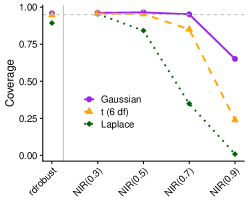
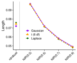
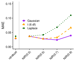
(a)	(b)	(c)

Figure 6: Simulation with a continuous running variable. We compare rdrobust and NIR with working noise model $\mathcal{N}(U_{i},\nu^{2})$ for $\nu\in\left\{0.3,0.5,0.7,0.9\right\}$ across three data generating processes wherein the true noise has variance $0.5^{2}$ and is Gaussian, t (with 6 degrees of freedom), and Laplace. NIR is well-specified only when $\nu=0.5$ and the noise model is Gaussian. We report (a) the coverage of confidence intervals, (b) the expected half-length of the confidence intervals, and (c) the mean absolute error.

Our evaluation proceeds as in Section 8.1 and the results are shown in Figure 6. rdrobust performs well across all three scenarios and sets a benchmark (even if it has some undercoverage with Laplace noise). With this standard in mind, we discuss the robustness of our proposed randomization-based approach when confronted with a misspecified noise model. We begin by examining the situation where the true noise model is Gaussian. Then, NIR has the correct (95$\%$) coverage for $\nu\in\left\{0.3,0.5,0.7\right\}$. Our theoretical results provide justification for $\nu=0.5$ (well-specification), and $\nu=0.3$ (underestimated noise-level as in Proposition 9). Coverage for $\nu=0.7$ in the simulation is not justified theoretically, but demonstrates some robustness of NIR to the specification of the noise level. On the other hand, for $\nu=0.9$, the coverage of NIR drops to roughly 65$\%$, showing that NIR is not robust to substantial overestimation of the noise level. The expected half-length of NIR confidence intervals is decreasing in $\nu$. The MAE exhibits a trade-off behavior, being minimized at $\nu=0.7$, decreasing before this point, and then increasing thereafter. This suggests that for point estimation (rather than inference), $\nu$ acts similarly to a standard bias-variance trade-off parameter. NIR is also moderately robust to misspecification of the shape of the noise distribution: NIR with $\nu=0.3$ attains 95$\%$ coverage with Laplace noise, and NIR with $\nu\in\left\{0.3,0.5\right\}$ attains nominal coverage with t-noise. However, when both the noise level and the shape of the noise distribution are strongly misspecified, the coverage of NIR can be very low.

The results of this simulation study suggest that NIR is robust to moderate misspecification of the noise model. In applications, one should err toward underestimating the noise level if possible.

9 Discussion

Informal descriptions of regression discontinuity designs often appeal to an analogy to a local randomized experiment, whereby units near the cutoff are as if randomly assigned to treatment. In perhaps the most common version of this analogy, one posits that units near the cutoff have had their running variable randomized (Cattaneo, Frandsen, and Titiunik, 2015). However, this analogy is typically undermined by the relevance of the running variable to the outcome—even within a region near the cutoff. Here, we proposed a new approach to inference in regression discontinuity designs that formalizes measurement error or other exogenous noise in the running variable $Z_{i}$ to capture the stochastic nature of the assignment mechanism in regression discontinuity designs. In the presence of measurement error, units are indeed randomly assigned to treatment—but with unknown, heterogeneous probabilities determined by a latent variable of which $Z_{i}$ is a noisy measure. Our results suggest that the pursuit of randomization-based inference in regression discontinuity designs may be practical in applications—concerns about power need not necessarily get in the way of a statistician who would prefer to rely on randomization-based inference for conceptual reasons.

Regression discontinuity designs with known or estimable measurement error in the running variable arise in many settings. We have already considered applications to educational and biomedical tests. Public policies that target interventions based on, e.g., proxy means testing (Alatas et al., 2012) may also readily admit analysis with the noise-induced randomization approach. Even data ostensibly arising from a complete census of a population may have measurement error in population totals or characteristics (Fraga and Merseth, 2016). Furthermore, this approach is applicable to settings where thresholds for statistical significance are used to make numerous decisions.

Software

All numerical results in this paper are reproducible with the code in the following Github repository: https://github.com/nignatiadis/noise-induced-randomization-paper.
We provide an implementation of NIR as a package in the Julia programming language (Bezanson et al., 2017) that depends, among others, on JuMP.jl (Dunning et al., 2017).

Appendix A Additional figures

Figure S1: Graphical illustration of the sharp regression discontinuity design in which treatment is assigned as a function of the latent variable $U$. $U$ is unobserved and the analyst only observes $Z$, a noisy measurement of $U$. We contrast the above causal diagram with the causal diagram underlying noise-induced randomization (Figure 1). In the latter case (noise-induced randomization), $Z$ is the running variable and the noise in $p(\cdot\,\big{|}\,\cdot)$ makes the inference task easier, that is, the regression discontinuity design becomes more akin to a randomized controlled trial. In the former case (not studied in this paper), the more noise there is in $p(\cdot\,\big{|}\,\cdot)$, the more challenging the causal inference task becomes.

Appendix B Proofs

B.1 Proof of Proposition 1

Proof:.

Conditioning on the latent variable $U$, we find that

$$\mathbb{E}\left[\gamma_{+}(Z)Y\,\big{|}\,U\right] \stackrel{{\scriptstyle(i)}}{{=}}\mathbb{E}\left[\gamma_{+}(Z)Y\cdot 1\left(\left\{Z\geq c\right\}\right)\,\big{|}\,U\right]$$

$$\stackrel{{\scriptstyle(ii)}}{{=}}\mathbb{E}\left[\gamma_{+}(Z)Y(1)\cdot 1\left(\left\{Z\geq c\right\}\right)\,\big{|}\,U\right]$$

$$\stackrel{{\scriptstyle(iii)}}{{=}}\underbrace{\mathbb{E}\left[Y(1)\,\big{|}\,U\right]}_{\alpha_{(1)}(U)}\underbrace{\mathbb{E}\left[\gamma_{+}(Z)1\left(\left\{Z\geq c\right\}\right)\,\big{|}\,U\right]}_{h(U,\gamma_{+})=\int\gamma_{+}(z)p(z\;|\;U)\,d\lambda(z)}$$

In $(i)$ we used that $\gamma_{+}(z)=0$ for $z<c$, in $(ii)$ we used the fact that $Y=Y(1)$ for $Z\geq c$ by Assumption 1 and in $(iii)$ we used exogeneity of the noise (Assumption 3). Finally, the expression for $\mathbb{E}\left[\gamma_{+}(Z)1\left(\left\{Z\geq c\right\}\right)\,\big{|}\,U\right]=\mathbb{E}\left[\gamma_{+}(Z)\,\big{|}\,U\right]$ follows from Assumption 2. By iterated expectation we thus find that $\mathbb{E}\left[\gamma_{+}(Z)Y\right]=\mathbb{E}\left[\alpha_{(1)}(U)h(U,\gamma_{+})\right]$. The proof for $\gamma_{-}$ is analogous. ∎

B.2 Proof of Corollary 3

Proof.

Noting that $\tau(U)=\alpha_{(1)}(U)-\alpha_{(0)}(U)$, this is proved by direct algebraic manipulation. ∎

B.3 Proof of Theorem 4

Proof.

Notation: We write $\mathbb{E}_{n}\left[\cdot\right]$ to denote empirical averages, i.e., for a function $h(\cdot$), we write:

$$\mathbb{E}_{n}\left[h(Z_{i})\right]=\frac{1}{n}\sum_{i=1}^{n}h(Z_{i}).$$

We omit dependence on $n$ of the weighting kernels. We only prove a central limit theorem for $\hat{\mu}_{\gamma,+}$. The CLT for $\hat{\mu}_{\gamma,-}$ and $\hat{\tau}_{\gamma}=\hat{\mu}_{\gamma,+}-\hat{\mu}_{\gamma,-}$ follow similarly.

CLT for $\sum_{i}\gamma_{+}(Z_{i})\left(Y_{i}(1)-\mu_{\gamma,+}\right)$: We seek to prove the following central limit theorem:

$$\frac{\sum_{i=1}^{n}\gamma_{+}(Z_{i})(Y_{i}(1)-\mu_{\gamma,+})}{\sqrt{n\mathbb{E}\left[\gamma_{+}(Z_{i})^{2}\left(Y_{i}(1)-\mu_{\gamma,+}\right)^{2}\right]}}\Rightarrow\mathcal{N}\left(0,1\right).$$

We first note that the numerator has expectation $0$, since:

$$\mathbb{E}\left[\gamma_{+}(Z_{i})(Y_{i}(1)-\mu_{\gamma,+})\right]=\mathbb{E}\left[\gamma_{+}(Z_{i})Y_{i}(1)\right]-\mathbb{E}\left[\gamma_{+}(Z_{i})\right]\frac{\mathbb{E}\left[\gamma_{+}(Z_{i})Y_{i}(1)\right]}{\mathbb{E}\left[\gamma_{+}(Z_{i})\right]}=0.$$

In the last step, we used the fact that by (11),(10):

$$\mu_{\gamma,+}=\frac{\mathbb{E}\left[\alpha_{(1)}(U)h(U,\;\gamma_{+})\right]}{\mathbb{E}\left[h(U,\;\gamma_{+})\right]}.$$ (S1)

But by Proposition 1 we also have that $\mathbb{E}\left[\alpha_{(1)}(U)h(U,\;\gamma_{+})\right]=\mathbb{E}\left[\gamma_{+}(Z_{i})Y_{i}(1)\right]$, while an analogous argument as in the proof of Proposition 1 demonstrates that $\mathbb{E}\left[h(U,\;\gamma_{+})\right]=\mathbb{E}\left[\gamma_{+}(Z_{i})\right]$.

Next we will check the condition of Lyapunov’s central limit theorem. Let $\underaccent{\bar}{\sigma}^{2}:=\inf_{z}\operatorname{Var}\left[Y_{i}\,\big{|}\,Z_{i}=z\right]>0$.

$$\operatorname{Var}\left[\gamma_{+}(Z_{i})\left(Y_{i}(1)-\mu_{\gamma,+}\right)\right] \geq\mathbb{E}\left[\operatorname{Var}\left[\gamma_{+}(Z_{i})\left(Y_{i}(1)-\mu_{\gamma,+}\right)\,\big{|}\,Z_{i}\right]\right]$$ (S2)

$$=\mathbb{E}\left[\gamma_{+}(Z_{i})^{2}\operatorname{Var}\left[Y_{i}(1)-\mu_{\gamma,+}\,\big{|}\,Z_{i}\right]\right]$$

$$=\mathbb{E}\left[\gamma_{+}(Z_{i})^{2}\operatorname{Var}\left[Y_{i}(1)\,\big{|}\,Z_{i}\right]\right]$$

$$=\mathbb{E}\left[\gamma_{+}(Z_{i})^{2}\operatorname{Var}\left[Y_{i}\,\big{|}\,Z_{i}\right]\right]$$

$$\geq\underaccent{\bar}{\sigma}^{2}\mathbb{E}\left[\gamma_{+}(Z_{i})^{2}\right].$$

In the penultimate line we used the fact that $Y_{i}(1)=Y_{i}$ on $\left\{Z_{i}\geq c\right\}$ and that $\gamma_{+}(z)=0$ for $z<c$. We next bound $\mu_{\gamma,+}$ in (S1). First, since $Y_{i}\in[0,1]$ by Assumption 4, it also follows that $\alpha_{(1)}(U)\in[0,1]$ almost surely. Thus:

$$\left\lvert\mu_{\gamma,+}\right\rvert=\left\lvert\frac{\mathbb{E}\left[\alpha_{(1)}(U)h(U,\;\gamma_{+})\right]}{\mathbb{E}\left[\gamma_{+}(Z_{i})\right]}\right\rvert\leq\frac{\mathbb{E}\left[\left\lvert h(U,\;\gamma_{+})\right\rvert\right]}{\mathbb{E}\left[\gamma_{+}(Z_{i})\right]}\leq\frac{\sup_{u}\left\lvert h(u,\;\gamma_{+})\right\rvert}{{\mathbb{E}\left[\gamma_{+}(Z_{i})\right]}}\leq C^{\prime},$$

for $n$ large enough. Then, for $q>0$ (and $n$ large enough) we have that:

$$\mathbb{E}\left[\left\lvert\gamma_{+}(Z_{i})\left(Y_{i}(1)-\mu_{\gamma,+}\right)\right\rvert^{2+q}\right] \leq(C^{\prime}+1)^{2+q}\mathbb{E}\left[\left\lvert\gamma_{+}(Z_{i})\right\rvert^{2+q}\right]$$

$$\leq(C^{\prime}+1)^{2+q}\cdot\sup_{z}\left\lvert\gamma_{+}(z)\right\rvert^{q}\cdot\mathbb{E}\left[\gamma_{+}(Z_{i})^{2}\right].$$

So:

$$\frac{n\mathbb{E}\left[\left\lvert\gamma_{+}(Z_{i})\left(Y_{i}(1)-\mu_{\gamma,+}\right)\right\rvert^{2+q}\right]}{\left(n\operatorname{Var}\left[\gamma_{+}(Z_{i})\left(Y_{i}(1)-\mu_{\gamma,+}\right)\right]\right)^{(2+q)/2}} \leq\frac{(C^{\prime}+1)^{2+q}\cdot\sup_{z}\left\lvert\gamma_{+}(z)\right\rvert^{q}\cdot\mathbb{E}\left[\gamma_{+}(Z_{i})^{2}\right]}{n^{q/2}\cdot\underaccent{\bar}{\sigma}^{2+q}\cdot\mathbb{E}\left[\gamma_{+}(Z_{i})^{2}\right]^{(2+q)/2}}$$

$$\leq\left(\frac{C^{\prime}+1}{\underaccent{\bar}{\sigma}}\right)^{2+q}\cdot\frac{\sup_{z}\left\lvert\gamma_{+}(z)\right\rvert^{q}}{n^{q/2}\cdot\mathbb{E}\left[\gamma_{+}(Z_{i})^{2}\right]^{q/2}}$$

$$\leq\left(\frac{C^{\prime}+1}{\underaccent{\bar}{\sigma}}\right)^{2+q}\cdot\frac{\sup_{z}\left\lvert\gamma_{+}(z)\right\rvert^{q}}{n^{q/2}\mathbb{E}\left[\gamma_{+}(Z_{i})\right]^{q}}$$

$$\leq\left(\frac{C^{\prime}+1}{\underaccent{\bar}{\sigma}}\right)^{2+q}\cdot\left(Cn^{\beta-1/2}\right)^{q}\to 0\text{ as }n\to\infty.$$

This proves the central limit theorem.

Estimation of normalization factor: Here we prove that $\mathbb{E}_{n}\left[\gamma_{+}(Z_{i})\right]\big{/}\mathbb{E}\left[\gamma_{+}(Z_{i})\right]=1+o_{\mathbb{P}}(1)$. For any $\varepsilon>0$, by Chebyshev’s inequality:

$$\mathbb{P}\left[\left\lvert\mathbb{E}_{n}\left[\gamma_{+}(Z_{i})\right]-\mathbb{E}\left[\gamma_{+}(Z_{i})\right]\right\rvert\geq\varepsilon\mathbb{E}\left[\gamma_{+}(Z_{i})\right]\right] \leq\frac{\operatorname{Var}\left[\gamma_{+}(Z_{i})\right]}{n\varepsilon^{2}\mathbb{E}\left[\gamma_{+}(Z_{i})\right]^{2}}$$

$$\leq\frac{\sup_{z}\gamma_{+}(z)^{2}}{n\varepsilon^{2}\mathbb{E}\left[\gamma_{+}(Z_{i})\right]^{2}}$$

$$\leq\left(\frac{C}{\varepsilon}\cdot n^{\beta-1/2}\right)^{2}\to 0\text{ as }n\to\infty.$$

CLT for $\hat{\mu}_{\gamma,+}$: Note that

$$\hat{\mu}_{\gamma,+}-\mu_{\gamma,+}=\sum_{i=1}^{n}\gamma_{+}(Z_{i})(Y_{i}(1)-\mu_{\gamma,+})\big{/}\sum_{i=1}^{n}\gamma_{+}(Z_{i}).$$

The above display, along with our preceding result, and Slutsky yield the CLT:

$$\frac{\sqrt{n}\left(\hat{\mu}_{\gamma,+}-\mu_{\gamma,+}\right)}{\sqrt{\mathbb{E}\left[\gamma_{+}(Z_{i})^{2}\left(Y_{i}(1)-\mu_{\gamma,+}\right)^{2}\right]\big{/}\mathbb{E}\left[\gamma_{+}(Z_{i})\right]^{2}}}\Rightarrow\mathcal{N}\left(0,1\right).$$

∎

B.4 Proof of Proposition 5

Proof.

The proof here continues from the argument used for the proof of Theorem 4. As we did there, we only prove the result for the variance of $\hat{\mu}_{\gamma,+}$, the result for $\hat{\tau}_{\gamma}$ follows analogously. In the proof of Theorem 4 we already showed that $\mathbb{E}_{n}\left[\gamma_{+}(Z_{i})\right]\big{/}\mathbb{E}\left[\gamma_{+}(Z_{i})\right]=1+o_{\mathbb{P}}(1)$. It thus suffices to show that:

$$\mathbb{E}_{n}\left[\gamma_{+}(Z_{i})^{2}\left(Y_{i}(1)-\hat{\mu}_{\gamma,+}\right)^{2}\right]\big{/}\mathbb{E}\left[\gamma_{+}(Z_{i})^{2}\left(Y_{i}(1)-\mu_{\gamma,+}\right)^{2}\right]=1+o_{\mathbb{P}}(1).$$ (S3)

We start by arguing that:

$$\mathbb{E}_{n}\left[\gamma_{+}(Z_{i})^{2}\left(Y_{i}(1)-\mu_{\gamma,+}\right)^{2}\right]\big{/}\mathbb{E}\left[\gamma_{+}(Z_{i})^{2}\left(Y_{i}(1)-\mu_{\gamma,+}\right)^{2}\right]=1+o_{\mathbb{P}}(1).$$ (S4)

First:

$$\operatorname{Var}\left[\frac{\mathbb{E}_{n}\left[\gamma_{+}(Z_{i})^{2}\left(Y_{i}(1)-\mu_{\gamma,+}\right)^{2}\right]}{\mathbb{E}\left[\gamma_{+}(Z_{i})^{2}\left(Y_{i}(1)-\mu_{\gamma,+}\right)^{2}\right]}\right] =\frac{\operatorname{Var}\left[\gamma_{+}(Z_{i})^{2}\left(Y_{i}(1)-\mu_{\gamma,+}\right)^{2}\right]}{n\cdot\mathbb{E}\left[\gamma_{+}(Z_{i})^{2}\left(Y_{i}(1)-\mu_{\gamma,+}\right)^{2}\right]^{2}}$$

$$\leq\frac{\mathbb{E}\left[\left\{\gamma_{+}(Z_{i})^{2}\left(Y_{i}(1)-\mu_{\gamma,+}\right)^{2}\right\}\cdot\left\{\gamma_{+}(Z_{i})^{2}\left(Y_{i}(1)-\mu_{\gamma,+}\right)^{2}\right\}\right]}{n\cdot\mathbb{E}\left[\gamma_{+}(Z_{i})^{2}\left(Y_{i}(1)-\mu_{\gamma,+}\right)^{2}\right]^{2}}$$

$$\leq\frac{(C^{\prime}+1)^{2}\sup_{z}\left\lvert\gamma_{+}(z)\right\rvert^{2}}{n\mathbb{E}\left[\gamma_{+}(Z_{i})^{2}\left(Y_{i}(1)-\mu_{\gamma,+}\right)^{2}\right]}\to 0\text{ as }n\to\infty.$$

Note that we verified that the last expression converges to $0$ as $n\to\infty$ during the verification of Lyapunov’s condition in the proof of Theorem 4. It follows that the asymptotic convergence in (S4) holds in $L^{2}$, thus also in probability. It remains to show that the feasible estimator in (S3) is asymptotically equivalent. We have the decomposition:

$$\gamma_{+}(Z_{i})^{2}\left(Y_{i}(1)-\widehat{\mu}_{\gamma,+}\right)^{2}-\gamma_{+}(Z_{i})^{2}\left(Y_{i}(1)-\mu_{\gamma,+}\right)^{2}$$

$$= \gamma_{+}(Z_{i})^{2}\left(\widehat{\mu}_{\gamma,+}-\mu_{\gamma,+}\right)^{2}+2\gamma_{+}(Z_{i})^{2}\left(Y_{i}(1)-\mu_{\gamma,+}\right)\left(\mu_{\gamma,+}-\widehat{\mu}_{\gamma,+}\right).$$

From the CLT of Theorem 4, we know that:

$$\left(\hat{\mu}_{\gamma,+}-\mu_{\gamma,+}\right)^{2}=O_{\mathbb{P}}\left(n^{-1}\mathbb{E}\left[\gamma_{+}(Z_{i})^{2}\left(Y_{i}(1)-\mu_{\gamma,+}\right)^{2}\right]\bigg{/}\mathbb{E}\left[\gamma_{+}(Z_{i})\right]^{2}\right)=O_{\mathbb{P}}\left(n^{-1+2\beta}\right)=o_{\mathbb{P}}(1),$$

and so:

$$\frac{\mathbb{E}_{n}\left[\gamma_{+}(Z_{i})^{2}\right]}{\mathbb{E}\left[\gamma_{+}(Z_{i})^{2}\left(Y_{i}(1)-\mu_{\gamma,+}\right)^{2}\right]}\cdot\left(\widehat{\mu}_{\gamma,+}-\mu_{\gamma,+}\right)^{2}=O_{\mathbb{P}}(1)\cdot o_{\mathbb{P}}(1)=o_{\mathbb{P}}(1).$$

The fact that the first term is $O_{\mathbb{P}}(1)$ follows by arguing with Chebyshev’s inequality. First note that from (S2), we know that $\mathbb{E}[\gamma_{+}(Z_{i})^{2}\left(Y_{i}(1)-\mu_{\gamma,+}\right)^{2}]\geq\underaccent{\bar}{\sigma}^{2}\mathbb{E}[\gamma_{+}(Z_{i})^{2}]$ and so it suffices to show that $\mathbb{E}_{n}\left[\gamma_{+}(Z_{i})^{2}\right]/\mathbb{E}\left[\gamma_{+}(Z_{i})^{2}\right]$ is $O_{\mathbb{P}}(1)$. Indeed this term is also $1+o_{\mathbb{P}}(1)$, since for any $\varepsilon>0$:

$$\mathbb{P}\left[\left\lvert\mathbb{E}_{n}\left[\gamma_{+}(Z_{i})^{2}\right]-\mathbb{E}\left[\gamma_{+}(Z_{i})^{2}\right]\right\rvert\geq\varepsilon\mathbb{E}\left[\gamma_{+}(Z_{i})^{2}\right]\right] \leq\frac{\operatorname{Var}\left[\gamma_{+}(Z_{i})^{2}\right]}{n\varepsilon^{2}\mathbb{E}\left[\gamma_{+}(Z_{i})^{2}\right]^{2}}$$

$$\leq\frac{\sup_{z}\gamma_{+}(z)^{2}}{n\varepsilon^{2}\mathbb{E}\left[\gamma_{+}(Z_{i})\right]^{2}}\cdot\frac{\mathbb{E}\left[\gamma_{+}(Z_{i})^{2}\right]}{\mathbb{E}\left[\gamma_{+}(Z_{i})^{2}\right]}$$

$$\leq\left(\frac{C}{\varepsilon}\cdot n^{\beta-1/2}\right)^{2}\to 0\text{ as }n\to\infty.$$

This proves the first term is negligible. To show that the second term is negligible, our basic argument is that

$$\frac{\mathbb{E}_{n}\left[\gamma_{+}(Z_{i})^{2}\left(Y_{i}(1)-\mu_{\gamma,+}\right)\right]}{\mathbb{E}\left[\gamma_{+}(Z_{i})^{2}\left(Y_{i}(1)-\mu_{\gamma,+}\right)^{2}\right]}\cdot\left(\widehat{\mu}_{\gamma,+}-\mu_{\gamma,+}\right)=O_{\mathbb{P}}(1)\cdot o_{\mathbb{P}}(1)=o_{\mathbb{P}}(1),$$

and it remains to prove that the first term is indeed $O_{\mathbb{P}}(1)$. By Cauchy-Schwarz

$$\left\lvert\mathbb{E}_{n}\left[\gamma_{+}(Z_{i})^{2}\left(Y_{i}(1)-\mu_{\gamma,+}\right)\right]\right\rvert =\left\lvert\mathbb{E}_{n}\left[\gamma_{+}(Z_{i})\cdot\gamma_{+}(Z_{i})\left(Y_{i}(1)-\mu_{\gamma,+}\right)\right]\right\rvert$$

$$\leq\left(\mathbb{E}_{n}\left[\gamma_{+}(Z_{i})^{2}\right]\right)^{1/2}\left(\mathbb{E}_{n}\left[\gamma_{+}(Z_{i})^{2}\left(Y_{i}(1)-\mu_{\gamma,+}\right)^{2}\right]\right)^{1/2}$$

But the above is the product of two $O_{\mathbb{P}}(\mathbb{E}[\gamma_{+}(Z_{i})^{2}(Y_{i}(1)-\mu_{\gamma,+})^{2}]^{1/2})$ terms (as we showed above), so we conclude upon dividing by $\mathbb{E}[\gamma_{+}(Z_{i})^{2}(Y_{i}(1)-\mu_{\gamma,+})^{2}]$. ∎

B.5 Proof of Proposition 6

Proof.

Consider the event $\left\{G\in\mathcal{G}_{n}\right\}$. On this event, by definition we have $\left\lvert b_{\gamma}\right\rvert\leq\widehat{B}_{\gamma,M}$ This implies that $\left\{G\in\mathcal{G}_{n}\right\}\subset\{\left\lvert b_{\gamma}\right\rvert\leq\widehat{B}_{\gamma,M}\}$ and so $\mathbb{P}[\left\lvert b_{\gamma}\right\rvert\leq\widehat{B}_{\gamma,M}]\geq\mathbb{P}\left[G\in\mathcal{G}_{n}\right]$. It thus suffices to show that the RHS converges to $1$ as $n\to\infty$. By construction of $\mathcal{G}_{n}$ in (18) and Massart’s tight constant for the DKW inequality [Massart, 1990], it holds that

$$\mathbb{P}\left[G\in\mathcal{G}_{n}\right]\geq\mathbb{P}\left[\sup_{t\in\mathbb{R}}\left\lvert F(t)-\widehat{F}_{n}(t)\right\rvert\leq\sqrt{\log\left(2/\alpha_{n}\right)\big{/}(2n)}\right]\geq 1-\alpha_{n}.$$

Since $\alpha_{n}\to 0$, we conclude the proof. ∎

B.6 Proof of Corollary 7

By Theorem 4, Proposition 5, and Slutsky, we have that

$$\frac{\sqrt{n}\left(\hat{\tau}_{\gamma}-\tau_{w}-b_{\gamma}\right)}{\widehat{V}_{\gamma}^{1/2}}\Rightarrow\mathcal{N}\left(0,1\right),$$

where $b_{\gamma}=\theta_{\gamma}-\tau_{w}$ by definition. So, letting $\tilde{Z}\sim\mathcal{N}\left(0,1\right)$ independent of everything else:

$$\mathbb{P}\left[\tau_{w}\in\hat{\tau}_{\gamma}\pm\ell_{\alpha}\right] =\mathbb{P}\left[-\ell_{\alpha}-b_{\gamma}\leq\hat{\tau}_{\gamma}-\tau_{w}-b_{\gamma}\leq\ell_{\alpha}-b_{\gamma}\right]$$

$$=\mathbb{P}\left[-\sqrt{n}\widehat{V}_{\gamma}^{-1/2}\left(\ell_{\alpha}+b_{\gamma}\right)\leq\sqrt{n}\widehat{V}_{\gamma}^{-1/2}\left(\hat{\tau}_{\gamma}-\tau_{w}-b_{\gamma}\right)\leq\sqrt{n}\widehat{V}_{\gamma}^{-1/2}\left(\ell_{\alpha}-b_{\gamma}\right)\right]$$

$$\stackrel{{\scriptstyle(i)}}{{=}}\mathbb{E}\left[\mathbb{P}\left[-\sqrt{n}\widehat{V}_{\gamma}^{-1/2}\left(\ell_{\alpha}+b_{\gamma}\right)\leq\tilde{Z}\leq\sqrt{n}\widehat{V}_{\gamma}^{-1/2}\left(\ell_{\alpha}-b_{\gamma}\right)\,\,\big{|}\,\,\widehat{V}_{\gamma},\widehat{B}_{\gamma,M},\hat{\tau}_{\gamma}\right]\right]+o(1)$$

$$=\mathbb{E}\left[\mathbb{P}\left[-\ell_{\alpha}\leq b_{\gamma}+n^{-1/2}\widehat{V}_{\gamma}^{1/2}\tilde{Z}\leq\ell_{\alpha}\,\,\big{|}\,\,\widehat{V}_{\gamma},\widehat{B}_{\gamma,M},\hat{\tau}_{\gamma}\right]\right]+o(1)$$

$$\stackrel{{\scriptstyle(ii)}}{{\geq}}\mathbb{E}\left[1-\alpha\right]+o(1)$$

$$=1-\alpha+o(1).$$

In $(i)$ we used the fact that the central limit theorem implies that the distribution function of the (asymptotic) pivot converges to the standard normal distribution function $\Phi(\cdot)$ uniformly. In $(ii)$ we used the definition of $\ell_{\alpha}$ in (21) and the fact that $\mathbb{P}[|b_{\gamma}|\leq\widehat{B}_{\gamma,M}]\rightarrow 1$ as $n\to\infty$.

B.7 Proof of Corollary 8

Let $\tau_{h,+}$ be defined as in (22). We will show that

$$\left\lvert\operatorname{Bias}\left[\gamma_{\pm},\,\tau_{h,+};\,\alpha_{(0)}(\cdot),\,\tau(\cdot),\,G\right]\right\rvert\leq\widehat{B}_{\gamma,M^{\prime}},$$

where $\widehat{B}_{\gamma,M^{\prime}}$ is defined as in (20) for the estimand $\tau_{w}$ (rather than $\tau_{h,+}$). We make this dependence explicit by writing $\widehat{B}_{\gamma,M^{\prime}}=\widehat{B}_{\gamma,M^{\prime},\tau_{w}}$. The “CATE heterogeneity bias” in Corollary 3 vanishes for $\tau_{h,+}$, i.e.,

$$\operatorname{Bias}\left[\gamma_{\pm},\,\tau_{h,+};\,\alpha_{(0)}(\cdot),\,\tau(\cdot),\,G\right]=\int\left(\frac{h(u,\;\gamma_{+})}{\mathbb{E}_{G}\left[h(U,\;\gamma_{+})\right]}-\frac{h(u,\;\gamma_{-})}{\mathbb{E}_{G}\left[h(U,\;\gamma_{-})\right]}\right)\alpha_{(0)}(u)\,dG(u).$$

However, the “CATE heterogeneity bias” also vanishes when $\tau(\cdot)\in\mathcal{T}_{0}$ (for any choice of estimand $\tau_{w}$), so that:

$$\left\lvert\operatorname{Bias}\left[\gamma_{\pm},\,\tau_{h,+};\,\alpha_{(0)}(\cdot),\,\tau(\cdot),\,G\right]\right\rvert=\left\lvert\operatorname{Bias}\left[\gamma_{\pm},\,\tau_{w};\,\alpha_{(0)}(\cdot),\,\tau(\cdot),\,G\right]\right\rvert,\text{ when }\tau(\cdot)\in\mathcal{T}_{0}.$$

Taking the supremum on the RHS over $\alpha_{(0)}(\cdot)\in[0,1]$, $\tau(\cdot)\in\mathcal{T}_{0}$ and $G\in\mathcal{G}_{n}$ demonstrates that:

$$\left\lvert\operatorname{Bias}\left[\gamma_{\pm},\,\tau_{h,+};\,\alpha_{(0)}(\cdot),\,\tau(\cdot),\,G\right]\right\rvert\leq\widehat{B}_{\gamma,0,\tau_{w}}\leq\widehat{B}_{\gamma,M^{\prime},\tau_{w}}.$$

The conclusion follows as in the proofs of Proposition 6 and Corollary 7.

B.8 Proof of Proposition 9

Proof.

To check this, note that we can generate $Z_{i}\,\big{|}\,U_{i}$ by first drawing $U_{i}^{\prime}\,\big{|}\,U_{i}$ with distribution $\pi(\cdot\,\big{|}\,U_{i})$, and then drawing $Z_{i}|U_{i}^{\prime}$ with distribution $\tilde{p}(\cdot\,\big{|}\,U_{i}^{\prime})$. The result of the proposition follows. ∎

Remark: Under this proposition, the interpretation of the latent variable changes: $U_{i}^{\prime}$ constructed in the proof is to be interpreted as the latent variable (and not the original $U_{i}$). Thus all our methodological analysis then goes through with $U_{i}$ replaced by $U_{i}^{\prime}$ (provided Assumption 3 holds with $U_{i}^{\prime}$).

B.9 Proof of Proposition 10

Proof.

We consider an alternative decomposition of the asymptotic bias that does not require Assumptions 2 and 3. We have that:

$$\mu_{\gamma,+} =\frac{\mathbb{E}\left[\gamma_{+}(Z)\mu_{(1)}(Z)\right]}{\mathbb{E}\left[\gamma_{+}(Z)\right]}$$

$$=\alpha_{0}+\tau_{c}+\frac{\int\gamma_{+}(z)\int a(u)p(z\mid u)dH(u)d\lambda(z)}{\int\gamma_{+}(z)f(z)d\lambda(z)}$$

$$=\alpha_{0}+\tau_{c}+\frac{\int a(u)\int\gamma_{+}(z)p(z\mid u)d\lambda(z)dH(u)}{\int\gamma_{+}(z)f(z)d\lambda(z)}$$

$$=\alpha_{0}+\tau_{c}+\frac{\int a(u)h(\gamma_{+},\;u)dH(u)}{\int\gamma_{+}(z)f(z)d\lambda(z)}$$

In the last step, it is important to emphasize that we apply the definition of $h(\gamma_{+},\;u)$ from (4) with the misspecified noise model $p(z\mid u)$. Arguing analogously for $\mu_{\gamma,-}$, we find that:

$$\theta_{\gamma}-\tau_{c} =\frac{\int a(u)h(\gamma_{+},\;u)dH(u)}{\int\gamma_{+}(z)f(z)d\lambda(z)}-\frac{\int a(u)h(\gamma_{-},\;u)dH(u)}{\int\gamma_{-}(z)f(z)d\lambda(z)}.$$

Define the functions:

$$\tilde{a}_{(0)}(\cdot):=\frac{\int\gamma_{-}(z)f_{H}(z)d\lambda(z)}{\int\gamma_{-}(z)f(z)d\lambda(z)}a(\cdot),\;\;\;\;\tilde{a}_{(1)}(\cdot):=\frac{\int\gamma_{+}(z)f_{H}(z)d\lambda(z)}{\int\gamma_{+}(z)f(z)d\lambda(z)}a(\cdot).$$

Then, we may write:

$$\theta_{\gamma}-\tau_{c} =\frac{\int\tilde{a}_{(1)}(u)h(\gamma_{+},\;u)dH(u)}{\int\gamma_{+}(z)f_{H}(z)d\lambda(z)}-\frac{\int\tilde{a}_{(0)}(u)h(\gamma_{-},\;u)dH(u)}{\int\gamma_{-}(z)f_{H}(z)d\lambda(z)}.$$

The above bias can be realized in (20) with $M=1$ by choosing $\alpha_{(0)}(\cdot)=\tilde{a}_{(0)}(\cdot)$, $\tau(\cdot)=\tilde{a}_{(1)}(\cdot)-\tilde{a}_{(0)}(\cdot)$, and $G=H$.

∎

B.10 Proof of Proposition 11

Proof.

We provide the argument for $\gamma_{+}=\gamma_{+}^{(n)}$; the argument for $\gamma_{-}=\gamma_{-}^{(n)}$ is analogous. First note that $\max_{z}\left\lvert\gamma_{+}(z)\right\rvert>0$ must hold, otherwise constraint (24c) of the optimization problem would not be satisfied. For convenience we define the events:

$$B_{n,1}=\left\{1/k<\bar{F}([c,\infty))<1-1/k,\;\sup_{u}\left\lvert\bar{w}(u)\right\rvert<k\right\},\;B_{n,2}=\left\{\int_{[c,\infty)}\gamma_{+}(z)dF(z)>\delta\right\}.$$

Next, let $C$ be as in (24e) and $\tilde{C}=C/\delta$. Then, on the event $B_{n,2}$ we have that:

$$\sup_{z}\left\lvert\gamma_{+}(z)\right\rvert\leq Cn^{\beta}\leq\tilde{C}n^{\beta}\cdot\delta<\tilde{C}n^{\beta}\int_{[c,\infty)}\gamma_{+}(z)dF(z).$$

Next, we will bound $\left\lvert h(u,\;\gamma_{+})\right\rvert$ on the event $B_{n,2}$. Consider the weighting kernel $\tilde{\gamma}_{+}(z)=\mathbf{1}(\left\{z\geq c\right\})/\bar{F}([c,\infty))$ and $\tilde{\gamma}_{-}(z)=\mathbf{1}(\left\{z<c\right\})/(1-\bar{F}([c,\infty)))$. This is a feasible solution under the constraints of optimization problem (24), since $\sup_{u}\left\lvert\tilde{\gamma}_{\diamond}(u)\right\rvert\leq 1/k\leq Cn^{\beta}$, $\diamond\in\left\{+,-\right\}$ on $B_{n,2}$ (and $n$ large enough), $\int\tilde{\gamma}_{-}(z)d\bar{F}(z)=1$ and $\int\tilde{\gamma}_{+}(z)d\bar{F}(z)=1$. We upper bound the objective of the optimization problem for that choice of weighting kernel. First, the variance-proxy term in the objective is equal to $\left[\bar{F}([c,\infty))^{-1}+(1-\bar{F}([c,\infty)))^{-1}\right]/n$ which is $\leq 2k/n\leq 1$ for $n$ large enough. On the other hand, note that we also have that:

$$\left\lvert h(u,\tilde{\gamma}_{+})\right\rvert=\left\lvert\bar{F}([c,\infty))^{-1}\cdot\int_{[c,\infty)}p(z\mid u)d\lambda(z)\right\rvert\leq\bar{F}([c,\infty))^{-1}\leq k,$$

and similarly $\left\lvert h(u,\tilde{\gamma}_{-})\right\rvert\leq k$. Hence by the triangle inequality we may bound the “$t_{1}$” term of the variance objective as $2k$, and similarly for the “$t_{2}$” term (recall that $\left\lvert\bar{w}(u)\right\rvert\leq k$ on $B_{n,2}$). Thus the objective of the whole optimization problem is upper bounded by $1+16k^{2}$. Thus, the objective for the optimal $\gamma_{\pm}$ in (24b) must be $\leq 1+16k^{2}$, which implies in particular for the optimal $\gamma_{\pm}$:

$$M\left\lvert h(u,\gamma_{+})-\bar{w}(u)\right\rvert\leq\sqrt{1+16k^{2}}\leq 5k.$$

Thus:

$$\sup_{u}\left\lvert h(u,\gamma_{+})\right\rvert\leq\sup_{u}\left\{\left\lvert h(u,\gamma_{+})-\bar{w}(u)\right\rvert+\left\lvert\bar{w}(u)\right\rvert\right\}\leq 5k/M+k\leq 6k/M.$$

We conclude that for $\tilde{C}$ as above and $\tilde{C}^{\prime}=6k/(M\delta)$, it holds that:

$$\mathbb{P}\left[\sup_{z}\left\lvert\gamma_{+}^{(n)}(z)\right\rvert<\tilde{C}n^{\beta}\mathbb{E}\left[\gamma_{+}^{(n)}(Z_{i})\right],\;\;\sup_{u}\left\lvert h(u,\;\gamma_{+}^{(n)})\right\rvert<\tilde{C}^{\prime}\mathbb{E}\left[\gamma_{+}^{(n)}(Z_{i})\right]\right]$$

$$\geq \mathbb{P}\left[B_{n,1}\cap B_{n,2}\right]\to 1\text{ as }n\to\infty.$$

∎

B.11 Proof of Proposition 12

Proof.

For the first result, note that $\mu_{(w)}(z)$ may in fact be extended to an analytic function across all of $\mathbb{C}$, cf. Kim [2014]. We proceed with the quantitative claims and first note that it suffices to consider the standard normal case, i.e., $\nu=1$. To see this, take $Z_{i}\,\big{|}\,U_{i}\sim\mathcal{N}\left(U_{i},\nu^{2}\right)$. Then $\tilde{Z}_{i}=Z_{i}/\nu_{i}\,\big{|}\,U_{i}\sim\mathcal{N}\left(U_{i}/\nu_{i},1\right)$ and we may apply the results to $\tilde{Z}_{i}$. Concretely, let $\tilde{m}:\mathbb{R}\mapsto\mathbb{R}$ be an arbitrary function and $m:z\mapsto\tilde{m}(z/\nu)=\tilde{m}(\tilde{z})$. This defines a bijection between functions that enables us to translate results for $\tilde{Z}_{i}$ into results for $Z_{i}$ and vice versa (by applying the chain rule). It only remains to express the density $\tilde{f}(\tilde{z})$ of $\tilde{Z}_{i}$ at $\tilde{z}=z/\nu$ in terms of the density $f$ of $Z_{i}$; by transformation we have $\tilde{f}(\tilde{z})=\nu\cdot f(z)$. Furthermore, we derive all of our results for $\mu_{(0)}(z)$; the arguments for $\mu_{(1)}(z)$ are identical.

Upper bound: Fix $\tilde{c}>0$. Let $\tilde{\alpha}_{(0)}(u)=\tilde{c}+\alpha_{(0)}(u)\in[\tilde{c},1+\tilde{c}]$. Let $H\ll G$ be the probability measure with

$$\frac{dH}{dG}(u)=\frac{\tilde{\alpha}_{(0)}(u)}{\int\tilde{\alpha}_{(0)}(u)dG(u)},$$

and write $h(z)=\int\varphi(z-u)dH(u)$. Then:

$$\mu_{(0)}(z)=\mathbb{E}\left[\alpha_{(0)}(U_{i})\,\big{|}\,Z_{i}=z\right]=\mathbb{E}\left[\tilde{\alpha}_{(0)}(U_{i})\,\big{|}\,Z_{i}=z\right]-\tilde{c}=\frac{h(z)\cdot\int\tilde{\alpha}_{(0)}(u)dG(u)}{f(z)}-\tilde{c}.$$

Taking the derivative:

$$\frac{d}{dz}\mu_{(0)}(z)=\int\tilde{\alpha}_{(0)}(u)dG(u)\cdot\left(\frac{h^{\prime}(z)}{f(z)}-\frac{h(z)}{f(z)}\cdot\frac{f^{\prime}(z)}{f(z)}\right)=\int\tilde{\alpha}_{(0)}(u)dG(u)\cdot\frac{h(z)}{f(z)}\cdot\left(\frac{h^{\prime}(z)}{h(z)}-\frac{f^{\prime}(z)}{f(z)}\right).$$

We next bound the three terms appearing in the expression above. First, we already saw that $\int\tilde{\alpha}_{(0)}(u)dG(u)\cdot\frac{h(z)}{f(z)}=\mu_{(0)}(z)+\tilde{c}$ with $\mu_{(0)}(z)\in[0,1]$ and so this term is upper bounded in absolute value by $1+\tilde{c}$. Next, by Lemma A.1. in Jiang and Zhang [2009] (which we state and prove at the end of this section for self-containedness) it holds that:

$$\left\lvert\frac{f^{\prime}(z)}{f(z)}\right\rvert\leq\sqrt{-\log(2\pi f^{2}(z))},\;\;\left\lvert\frac{h^{\prime}(z)}{h(z)}\right\rvert\leq\sqrt{-\log(2\pi h^{2}(z))}.$$

It remains to lower bound $h(z)/f(z)$:

$$h(z)=\frac{\int\tilde{\alpha}_{(0)}(u)\varphi(z-u)dG(u)}{\int\tilde{\alpha}_{(0)}(u)dG(u)}\geq\frac{\tilde{c}}{1+\tilde{c}}\cdot\int\varphi(z-u)dG(u)=\frac{\tilde{c}}{1+\tilde{c}}\cdot f(z).$$

Applying the triangle inequality and putting everything together:

$$\left\lvert\frac{d}{dz}\mu_{(0)}(z)\right\rvert\leq\inf_{\tilde{c}>0}\left\{(1+\tilde{c})\cdot\left(\sqrt{-\log(2\pi f^{2}(z))}+\sqrt{-\log\left(\frac{2\pi\tilde{c}^{2}}{(1+\tilde{c})^{2}}f^{2}(z)\right)}\right)\right\}.$$

Taking $\tilde{c}=1+\sqrt{2}$ and noting that $2(1+\tilde{c})<7$ leads to the bound:

$$\left\lvert\frac{d}{dz}\mu_{(0)}(z)\right\rvert\leq 7\sqrt{-\log(\pi f^{2}(z))}.$$

Continuing, the second derivative of $\mu_{(0)}(z)$ is equal to:

$$\mu_{(0)}^{\prime\prime}(z)=\left(\mu_{(0)}(z)+\tilde{c}\right)\cdot\left\{\left(\frac{h^{\prime\prime}(z)}{h(z)}+1\right)-\left(\frac{f^{\prime\prime}(z)}{f(z)}+1\right)\right\}-2\mu^{\prime}_{(0)}(z)\cdot\frac{f^{\prime}(z)}{f(z)}.$$

Applying Lemma A.1. in Jiang and Zhang [2009] a second time we find that:

$$0\leq\frac{f^{\prime\prime}(z)}{f(z)}+1\leq-\log(2\pi f^{2}(z)),\;\;0\leq\frac{h^{\prime\prime}(z)}{h(z)}+1\leq-\log(2\pi h^{2}(z)).$$

Using the fact that $\left\lvert\mu_{(0)}(z)+\tilde{c}\right\rvert\leq 1+\tilde{c}$, that we already bounded $|\mu_{(0)}^{\prime}(z)|$, $f^{\prime}(z)/f(z)$ above, and the triangle inequality we conclude.

Lower bound: Without loss of generality, we consider the case that $z=0$. Let $\delta_{u}$ denote the point mass measure at $\left\{u\right\}$. We take $G=\frac{1-w}{2}\cdot\left(\delta_{-t}+\delta_{t}\right)+w\cdot\delta_{0}$ for parameters $w\in[0,1]$, $t>0$ which we will specify later and $\alpha_{(0)}(u)=\mathbf{1}\left(u=0\right)$. Then:

$$f(z)=\frac{1-w}{2}\cdot\left(\varphi(z-t)+\varphi(z+t)\right)+w\cdot\varphi(z),\;\mu_{(0)}(z)=w\cdot\frac{\varphi(z)}{f(z)}.$$

To simplify notation we write $\mu(\cdot)=\mu_{(0)}(\cdot)$. By direct calculation we can verify that

$$\mu^{\prime\prime}(0)=-w\frac{\varphi(0)f(0)+\varphi(0)f^{\prime\prime}(0)}{f^{2}(0)},\;\;f^{\prime\prime}(0)=(1-w)(t^{2}-1)\varphi(t)-w\varphi(0).$$

Next choose $w=\varphi(t)$, so that $f(0)=(1+\varphi(0)-\varphi(t))\varphi(t)$ and

$$\mu^{\prime\prime}(0)=-\varphi(0)\frac{(1-\varphi(t))\cdot t^{2}}{(1+\varphi(0)-\varphi(t))^{2}}.$$

Finally, we pick $t$ so that $\varphi(t)=\rho$. It then holds in particular that $f(0)\geq\rho$ and using the fact that $\varphi(t)\in(0,1/\sqrt{2\pi}]$, we get:

$$\left\lvert\mu^{\prime\prime}(0)\right\rvert\geq\frac{1}{10}t^{2}=\frac{1}{10}(-\log(2\pi\rho^{2})).$$

∎

B.11.1 Lemma A.1. in Jiang and Zhang [2009]

Lemma A.1. (Jiang and Zhang [2009]).

Let $G$ be a distribution on $\mathbb{R}$, let $\varphi$ be the standard normal density function and let $f_{G}(z)=\int\varphi(z-u)dG(u)$ be the density of the convolution $G\star\varphi$. Then:

$$0\;\leq\;\left(\frac{f_{G}^{\prime}(z)}{f_{G}(z)}\right)^{2}\;\leq\;\frac{f_{G}^{\prime\prime}(z)}{f_{G}(z)}+1\;\leq\;-\log\left(2\pi f_{G}^{2}(z)\right).$$

Proof.

Let $U\sim G$ and $Z\mid U\sim\mathcal{N}(U,1)$. We may verify the following three equalities:

$$\mathbb{E}\left[U-z\mid Z=z\right]=\frac{f_{G}^{\prime}(z)}{f_{G}(z)},\;\;\mathbb{E}\left[(U-z)^{2}\mid Z=z\right]=\frac{f_{G}^{\prime\prime}(z)}{f_{G}(z)}+1,\;$$

$$\mathbb{E}\left[\sqrt{2\pi}\exp\left((U-z)^{2}/2\right)\mid Z=z\right]=1/f_{G}(z).$$

Then, by Jensen’s inequality:

$$\left(\frac{f_{G}^{\prime}(z)}{f_{G}(z)}\right)^{2}=\mathbb{E}\left[U-z\mid Z=z\right]^{2}\leq\mathbb{E}\left[(U-z)^{2}\mid Z=z\right]=\frac{f_{G}^{\prime\prime}(z)}{f_{G}(z)}+1.$$

Next, define the convex function $h(x)=\sqrt{2\pi}\exp(x/2)$ with inverse $h^{-1}(y)=\log(y^{2}/(2\pi))$. Applying Jensen’s inequality again, we see that:

$$\frac{f_{G}^{\prime\prime}(z)}{f_{G}(z)}+1\leq h^{-1}\left(\mathbb{E}\left[h\left((U-z)^{2}\right)\mid Z=z\right]\right)\;=\;h^{-1}(1/f_{G}(z))=-\log\left(2\pi f_{G}^{2}(z)\right).$$

∎

Appendix C Computational details

C.1 Computation of worst-case bias

C.1.1 Notation

In this section we explain how to compute the worst-case bias in (20). The main idea behind our optimization algorithm is to define $A_{(0)}$, resp. $T$ as the signed measure that is absolutely continuous with respect to $G$ with density $\alpha_{(0)}(u)$, resp. $\tau(u)$. We will parameterize the optimization problem in terms of optimization variables that represent $G$, $A_{(0)}$ and $T$. To simplify notation, we define the following linear functionals:

$$L_{h,+}(H) =\int h(u,\;\gamma_{+})dH(u),$$

$$L_{h,-}(H) =\int h(u,\;\gamma_{-})dH(u),$$

$$L_{w}(H) =\int w(u)dH(u).$$

Then we can write:

$$\operatorname{Bias}\left[\gamma_{\pm},\,\tau_{w};\,\alpha_{(0)}(\cdot),\,\tau(\cdot),\,G\right]=\frac{L_{h,+}(A_{(0)})+L_{h,+}(T)}{L_{h,+}(G)}-\frac{L_{h,-}(A_{(0)})}{L_{h,-}(G)}-\frac{L_{w}(T)}{L_{w}(G)},$$ (S5)

a sum-of-ratios of linear functionals. We propose solving:

$$\sup_{G,A_{(0)},T}\quad \frac{L_{h,+}(A_{(0)})+L_{h,+}(T)}{L_{h,+}(G)}-\frac{L_{h,-}(A_{(0)})}{L_{h,-}(G)}-\frac{L_{w}(T)}{L_{w}(G)}$$ (S6a)

s.t. $$G\in\mathcal{G}_{n},$$ (S6b)

$$0\leq\frac{dA_{(0)}}{dG}(u)\leq 1\text{ for all }u,$$ (S6c)

$$0\leq\frac{dT}{dG}(u)\leq 2M\text{ for all }u.$$ (S6d)

We explain why this problem is equivalent to the problem we care about solving in (20). There are two observations:

1. We first show that it suffices to reduce attention to $T(\cdot)$ satisfying (S6d) instead of more general $T(\cdot)$ that satisfy the heterogeneity constraint in (19). Fix $G$, $A_{(0)}$ and $T$ that are feasible for (20). Let $\bar{\tau}$ be such that $\left\lvert dT(u)/dG-\bar{\tau}\right\rvert\leq M$ and define $\check{T}=\bar{\tau}\cdot G+T$. Then $d\check{T}(u)/dG=dT(u)/dG+\bar{\tau}\in[0,\,2M]$. Hence $G,A_{(0)},\check{T}$ are also feasible. Furthermore, we may check that $(G,A_{(0)},T)$ and $(G,A_{(0)},\check{T})$ lead to the same value of the objective $\operatorname{Bias}\left[\gamma_{\pm},\,\tau_{w};\,\cdot,\cdot,\cdot\right]$ in (S5).

2. We next show that we may ignore the absolute value in (20). Fix feasible $G$, $A_{(0)}$ and $T$. Suppose we replace $A_{(0)}$ and $T$ by$\check{A}_{(0)}=G-A_{(0)}$ and $\check{T}=2M\cdot G-T$. Then $d\check{A}_{(0)}(u)/dG=1-dA_{(0)}(u)/dG\in[0,1]$, and so the constraint (S6c) will continue to be satisfied and similarly, $d\check{T}(u)/dG=2M-dT(u)/dG\in[0,2M]$, and so the constraint (S6d) will also continue to be satisfied. Hence $G$, $\check{A}_{(0)}$ and $\check{T}$ also are feasible and we may further check that the objective value switches sign compared to its original value and retains its absolute value. Thus optimization problem (S6) is implicitly maximizing the absolute value of the objective.

C.1.2 Optimizing the sum-of-ratios objective

We now explain how (S6) may be solved numerically. First, we may reduce the number of ratios in the objective by the Charnes and Cooper [1962] transformation, as follows:

$$\sup_{\check{G},\check{A}_{(0)},\check{T},\xi}\quad L_{h,+}(\check{A}_{(0)})+L_{h,+}(\check{T})-\frac{L_{h,-}(\check{A}_{(0)})}{L_{h,-}(\check{G})}-\frac{L_{w}(\check{T})}{L_{w}(\check{G})}$$ (S7a)

s.t. $$\check{G}\in\left\{\xi\cdot\tilde{G}:\tilde{G}\in\mathcal{G}_{n}\right\},$$ (S7b)

$$0\leq\frac{d\check{A}_{(0)}}{d\check{G}}(u)\leq 1\text{ for all }u,$$ (S7c)

$$0\leq\frac{d\check{T}}{d\check{G}}(u)\leq 2M\text{ for all }u,$$ (S7d)

$$L_{h,+}(\check{G})=1,$$ (S7e)

$$\xi\geq 0.$$ (S7f)

The optimization variables are $\xi\geq 0$, $\check{G}$, $\check{A}_{(0)}$, and $\check{T}$. Their interpretation is as follows: $\xi=1/L_{h,+}(G)$, $\check{G}=\xi\cdot G$, $\check{A}_{(0)}=\xi\cdot A_{(0)}$, and $\check{T}=\xi\cdot T$. Next consider solving (S7) subject to the additional linear constraints that

$$L_{h,-}(\check{G})=\zeta,\;\;L_{w}(\check{G})=\kappa,$$

for fixed values of $\zeta,\kappa$. In more detail, let:

$$\mathcal{L}(\zeta,\kappa)=\sup_{\check{G},\check{A}_{(0)},\check{T},\xi}\quad L_{h,+}(\check{A}_{(0)})+L_{h,+}(\check{T})-\frac{1}{\zeta}L_{h,-}(\check{A}_{(0)})-\frac{1}{\kappa}L_{w}(\check{T})$$ (S8a)

s.t. $$\eqref{eq:gcal_cc},\eqref{eq:A_0_constraint_cc},\eqref{eq:T_constraint_cc},\eqref{eq:unity_cc},\eqref{eq:nonneg_cc},$$ (S8b)

$$L_{h,-}(\check{G})=\zeta,$$ (S8c)

$$L_{w}(\check{G})=\kappa.$$ (S8d)

For fixed values of $\zeta,\kappa$, the above is a linear program. Thus we may solve (S7) by profiling over $\zeta$ and $\kappa$ and repeatedly solving (S8). Formally, let:

$$\underaccent{\bar}{\zeta}=\inf_{\check{G},\check{A}_{(0)},\check{T},\xi}\quad \left\{L_{h,-}(\check{G})\right\}\;\;\textrm{s.t. } \eqref{eq:gcal_cc},\eqref{eq:A_0_constraint_cc},\eqref{eq:T_constraint_cc},\eqref{eq:unity_cc},\eqref{eq:nonneg_cc},$$ (S9)

and $$\bar{\zeta}=\sup_{\check{G},\check{A}_{(0)},\check{T},\xi}\quad \left\{L_{h,-}(\check{G})\right\}\;\;\textrm{s.t. } \eqref{eq:gcal_cc},\eqref{eq:A_0_constraint_cc},\eqref{eq:T_constraint_cc},\eqref{eq:unity_cc},\eqref{eq:nonneg_cc}.$$

Furthermore, for $\zeta\in[\underaccent{\bar}{\zeta},\bar{\zeta}]$, let:

$$\underaccent{\bar}{\kappa}(\zeta)=\inf_{\check{G},\check{A}_{(0)},\check{T},\xi}\quad \left\{L_{w}(\check{G})\right\}\;\;\textrm{s.t. } L_{h,-}(\check{G})=\zeta,\;\eqref{eq:gcal_cc},\eqref{eq:A_0_constraint_cc},\eqref{eq:T_constraint_cc},\eqref{eq:unity_cc},\eqref{eq:nonneg_cc},$$ (S10)

and $$\bar{\kappa}(\zeta)=\sup_{\check{G},\check{A}_{(0)},\check{T},\xi}\quad \left\{L_{w}(\check{G})\right\}\;\;\textrm{s.t. } L_{h,-}(\check{G})=\zeta,\;\eqref{eq:gcal_cc},\eqref{eq:A_0_constraint_cc},\eqref{eq:T_constraint_cc},\eqref{eq:unity_cc},\eqref{eq:nonneg_cc}.$$

Then the worst-case bias we are interested in is equal to:

$$\sup\Big{\{}\sup\left\{\mathcal{L}(\zeta,\kappa)\;:\;\kappa\in\left[\,\underaccent{\bar}{\kappa}(\zeta),\;\bar{\kappa}(\zeta)\right]\right\}\;:\;\zeta\in\left[\,\underaccent{\bar}{\zeta},\;\bar{\zeta}\right]\Big{\}}.$$ (S11)

C.1.3 Discretization considerations

To turn the above construction into a practical computational algorithm, we need to solve optimization problems (S8), (S9), and (S10), as well as solve the profiling task (S11). We will achieve this by finely discretizing. We refer to Ignatiadis and Wager [2022, Supplement D] for a more detailed discussion regarding discretization considerations and describe our implementation choices here.

Instead of optimizing over the space of all distributions for the latent variable $U$, we optimize over all distributions supported on the equidistant finite grid from $a_{\text{min}}$ to $a_{\text{max}}$ with $B$ points:

$$\mathcal{K}(B,a_{\text{min}},a_{\text{max}})=\left\{a_{\text{min}},\,a_{\text{min}}+\frac{a_{\text{max}}-a_{\text{min}}}{B},\,a_{\text{min}}+2\frac{a_{\text{max}}-a_{\text{min}}}{B},\,\dotsc,\,a_{\text{max}}\right\}.$$ (S12)

Our default choice uses $B=499$, $a_{\text{min}}=\min\left\{Z_{1},\dotsc,Z_{n}\right\}$, $a_{\text{max}}=\max\left\{Z_{1},\dotsc,Z_{n}\right\}$ for Gaussian noise distributions and $B=399$, $a_{\text{min}}=10^{-4}$ and $a_{\text{max}}=1-10^{-4}$ for Binomial noise (the latter choice of $a_{\text{min}}$, $a_{\text{max}}$ for the Binomial empirical Bayes problem is used by default in Koenker and Gu [2017]).

By enumerating the grid elements as $\mathcal{K}(B,a_{\text{min}},a_{\text{max}})=\left\{u_{1},\dotsc,u_{B+1}\right\}$, we may represent every distribution $G$ supported on this set by the probabilities $g_{j}=\mathbb{P}_{G}\left[U=u_{j}\right]$ assigned to $u_{j}$. The $g_{j}$ lie on the probability simplex. Furthermore, we may represent $\check{G}$ by $\check{g}_{j}$, which satisfy:

$$\sum_{j=1}^{B+1}\check{g}_{j}=\xi,\;\check{g}_{j}\geq 0.$$

Analogously, we may represent $\check{T},\check{A}_{(0)}$ by $(B+1)$-dimensional vectors and we only need to apply the constraints in (S7c) and  (S7d) for $u\in\mathcal{K}(B,L,U)$. Hence, after the aforementioned discretization, all of  (S8), (S9), and (S10) turn into finite-dimensional linear programs that we optimize using the MOSEK solver [ApS, 2020].

To solve the profiling problem (S11), instead of considering all $\zeta\in[\underaccent{\bar}{\zeta},\bar{\zeta}]$, we only consider $\zeta\in\mathcal{K}(49,\underaccent{\bar}{\zeta},\bar{\zeta})$. Meanwhile, for each such $\zeta$ we discretize $[\underaccent{\bar}{\kappa}(\zeta),\bar{\kappa}(\zeta)]$ as an equidistant grid with distance between grid points of at most $\underaccent{\bar}{\zeta}/5$. Hence we solve the discretized (S11) by solving a finite number of linear programs.

C.2 Computation of worst-case curvature

The construction for optimizing the worst-case curvature is very similar to the construction in Supplement C.1, i.e., after profiling we reduce the optimization problem to a sequence of linear programming tasks. We provide a sketch here.

Our starting point is the ratio representation (25) of $\mu(\cdot)=\mu_{(w)}(\cdot)$ (omitting the subscript _(w) henceforth), which we may write as:

$$\mu(z)=\frac{N(z)}{D(z)},$$

where $N(\cdot)$, resp. $D(\cdot)$ are the numerator, resp. denominator in (25). Then, assuming $N(\cdot),D(\cdot)$ are twice differentiable, we get by the chain rule that:

$$\mu^{\prime\prime}(z)=\frac{N^{\prime\prime}(z)}{D(z)}-2\frac{N^{\prime}(z)D^{\prime}(z)}{D^{2}(z)}-\frac{N(z)D^{\prime\prime}(z)}{D^{2}(z)}+2\frac{N(z)(D^{\prime}(z))^{2}}{D(z)^{3}}.$$

The absolute value of the above is the quantity we seek to maximize. The critical observation now is that all of $D(z),D^{\prime}(z),D^{\prime\prime}(z)$ are linear functionals of $G$. Similarly, $N(z),N^{\prime}(z),N^{\prime\prime}(z)$ are linear functionals of $A$, defined as the measure $\ll G$ with $dA(u)/dG=\alpha_{(w)}(u)$. Applying the Charnes and Cooper [1962] transformation (as we did in Supplement C.1) we may rescale the optimization variables $G$ and $A$ as $\check{G},\check{A}$, such that $\int p(z\mid u)d\check{G}(u)=1$. Writing $\check{N}(\cdot),\check{D}(\cdot)$ for the corresponding numerator and denominator

$$\check{N}(\cdot)=\int p(\cdot\mid u)d\check{A}(u),\;\;\check{D}(\cdot)=\int p(\cdot\mid u)d\check{G}(u),$$

we get by the above transformation that $\check{D}(z)=1$, and hence:

$$\mu^{\prime\prime}(z)=\check{N}^{\prime\prime}(z)-2\check{N}^{\prime}(z)\check{D}^{\prime}(z)-\check{N}(z)\check{D}^{\prime\prime}(z)+2\check{N}(z)(\check{D}^{\prime}(z))^{2}.$$ (S13)

To conclude we use a profiling argument as in Supplement C.1. Concretely, fix $\kappa,\zeta$ and consider the linear (in the optimization variables) constraints:

$$\check{D}^{\prime}(z)=\zeta,\;\check{D}^{\prime\prime}(z)=\kappa.$$

Under these constraints, we have that:

$$\mu^{\prime\prime}(z)=\check{N}^{\prime\prime}(z)-2\zeta\check{N}^{\prime}(z)-\kappa\check{N}(z)+2\zeta^{2}\check{N}(z).$$

This objective is linear in the optimization variables (for fixed values of $\zeta,\kappa$) and so we can maximize/minimize it with respect to the constraints by linear programming.

References

- Alatas et al. [2012] Vivi Alatas, Abhijit Banerjee, Rema Hanna, Benjamin A Olken, and Julia Tobias. Targeting the poor: Evidence from a field experiment in Indonesia. American Economic Review, 102(4):1206–40, 2012.
- Angrist and Rokkanen [2015] Joshua D Angrist and Miikka Rokkanen. Wanna get away? Regression discontinuity estimation of exam school effects away from the cutoff. Journal of the American Statistical Association, 110(512):1331–1344, 2015.
- ApS [2020] MOSEK ApS. The MOSEK Optimization Suite Manual, Version 9.2, 2020. URL https://www.mosek.com/.
- Armstrong and Kolesár [2018] Timothy B Armstrong and Michal Kolesár. Optimal inference in a class of regression models. Econometrica, 86(2):655–683, 2018.
- Armstrong and Kolesár [2020] Timothy B Armstrong and Michal Kolesár. Simple and honest confidence intervals in nonparametric regression. Quantitative Economics, 11(1):1–39, 2020.
- Bartalotti et al. [2020] Otávio Bartalotti, Quentin Brummet, and Steven Dieterle. A correction for regression discontinuity designs with group-specific mismeasurement of the running variable. Journal of Business & Economic Statistics, pages 1–16, 2020.
- Benson [2007] Harold P Benson. A simplicial branch and bound duality-bounds algorithm for the linear sum-of-ratios problem. European Journal of Operational Research, 182(2):597–611, 2007.
- Bezanson et al. [2017] Jeff Bezanson, Alan Edelman, Stefan Karpinski, and Viral B Shah. Julia: A fresh approach to numerical computing. SIAM Review, 59(1):65–98, 2017.
- Bilodeau [1997] Martin Bilodeau. Estimating a multivariate treatment effect under a biased allocation rule. Communications in Statistics-Theory and Methods, 26(5):1119–1124, 1997.
- Bor et al. [2014] Jacob Bor, Ellen Moscoe, Portia Mutevedzi, Marie-Louise Newell, and Till Bärnighausen. Regression discontinuity designs in epidemiology: Causal inference without randomized trials. Epidemiology (Cambridge, Mass.), 25(5):729, 2014.
- Bor et al. [2017] Jacob Bor, Matthew P Fox, Sydney Rosen, Atheendar Venkataramani, Frank Tanser, Deenan Pillay, and Till Bärnighausen. Treatment eligibility and retention in clinical HIV care: A regression discontinuity study in South Africa. PLoS Medicine, 14(11), 2017.
- Branson et al. [2019] Zach Branson, Maxime Rischard, Luke Bornn, and Luke W Miratrix. A nonparametric Bayesian methodology for regression discontinuity designs. Journal of Statistical Planning and Inference, 202:14–30, 2019.
- Brinch et al. [2017] Christian N Brinch, Magne Mogstad, and Matthew Wiswall. Beyond LATE with a discrete instrument. Journal of Political Economy, 125(4):985–1039, 2017.
- Calonico et al. [2014] Sebastian Calonico, Matias D Cattaneo, and Rocío Titiunik. Robust nonparametric confidence intervals for regression-discontinuity designs. Econometrica, 82(6):2295–2326, 2014.
- Calonico et al. [2015] Sebastian Calonico, Matias D. Cattaneo, and Rocío Titiunik. rdrobust: An R Package for Robust Nonparametric Inference in Regression-Discontinuity Designs. The R Journal, 7(1):38–51, 2015.
- Calonico et al. [2018] Sebastian Calonico, Matias D Cattaneo, and Max H Farrell. On the effect of bias estimation on coverage accuracy in nonparametric inference. Journal of the American Statistical Association, 113(522):767–779, 2018.
- Candès et al. [2018] Emmanuel Candès, Yingying Fan, Lucas Janson, and Jinchi Lv. Panning for gold: ‘Model-X’ knockoffs for high dimensional controlled variable selection. Journal of the Royal Statistical Society Series B: Statistical Methodology, 80(3):551–577, 2018.
- Cattaneo et al. [2015] Matias D Cattaneo, Brigham R Frandsen, and Rocío Titiunik. Randomization inference in the regression discontinuity design: An application to party advantages in the US Senate. Journal of Causal Inference, 3(1):1–24, 2015.
- Caughey and Sekhon [2011] Devin Caughey and Jasjeet S Sekhon. Elections and the regression discontinuity design: Lessons from close US house races, 1942-2008. Political Analysis, 19(4):385–408, 2011.
- Charnes and Cooper [1962] A. Charnes and W. W. Cooper. Programming with linear fractional functionals. Naval Research Logistics Quarterly, 9(3‐4):181–186, 1962.
- Cheng et al. [1997] Ming-Yen Cheng, Jianqing Fan, and James S Marron. On automatic boundary corrections. The Annals of Statistics, 25(4):1691–1708, 1997.
- Cook [2008] Thomas D Cook. Waiting for life to arrive: A history of the regression-discontinuity design in psychology, statistics and economics. Journal of Econometrics, 142(2):636–654, 2008.
- Cooperman [2017] Alicia Dailey Cooperman. Randomization inference with rainfall data: Using historical weather patterns for variance estimation. Political Analysis, 25(3):277–288, 2017.
- Crump et al. [2009] Richard K Crump, V Joseph Hotz, Guido W Imbens, and Oscar A Mitnik. Dealing with limited overlap in estimation of average treatment effects. Biometrika, 96(1):187–199, 2009.
- Davezies and Le Barbanchon [2017] Laurent Davezies and Thomas Le Barbanchon. Regression discontinuity design with continuous measurement error in the running variable. Journal of Econometrics, 200(2):260–281, 2017.
- Dong and Kolesár [2023] Yingying Dong and Michal Kolesár. When can we ignore measurement error in the running variable? Journal of Applied Econometrics, 38(5):735–750, 2023.
- Dong and Lewbel [2015] Yingying Dong and Arthur Lewbel. Identifying the effect of changing the policy threshold in regression discontinuity models. Review of Economics and Statistics, 97(5):1081–1092, 2015.
- Dunning et al. [2017] Iain Dunning, Joey Huchette, and Miles Lubin. JuMP: A modeling language for mathematical optimization. SIAM Review, 59(2):295–320, 2017.
- Dwork and Roth [2013] Cynthia Dwork and Aaron Roth. The algorithmic foundations of differential privacy. Foundations and Trends® in Theoretical Computer Science, 9(3-4):211–407, 2013.
- Finkelstein et al. [1996a] Michael O Finkelstein, Bruce Levin, and Herbert Robbins. Clinical and prophylactic trials with assured new treatment for those at greater risk: I. A design proposal. American Journal of Public Health, 86(5):691–695, 1996a.
- Finkelstein et al. [1996b] Michael O Finkelstein, Bruce Levin, and Herbert Robbins. Clinical and prophylactic trials with assured new treatment for those at greater risk: II. Examples. American Journal of Public Health, 86(5):696–705, 1996b.
- Fraga and Merseth [2016] Bernard L Fraga and Julie Lee Merseth. Examining the causal impact of the voting rights act language minority provisions. Journal of Race, Ethnicity, and Politics, 1(1):31–59, 2016.
- Frangakis and Rubin [2002] Constantine E Frangakis and Donald B Rubin. Principal stratification in causal inference. Biometrics, 58(1):21–29, 2002.
- Ganong and Jäger [2018] Peter Ganong and Simon Jäger. A permutation test for the regression kink design. Journal of the American Statistical Association, 113(522):494–504, 2018.
- Gelman and Imbens [2019] Andrew Gelman and Guido Imbens. Why high-order polynomials should not be used in regression discontinuity designs. Journal of Business & Economic Statistics, 37(3):447–456, 2019.
- Geneletti et al. [2015] Sara Geneletti, Aidan G. O’Keeffe, Linda D. Sharples, Sylvia Richardson, and Gianluca Baio. Bayesian regression discontinuity designs: Incorporating clinical knowledge in the causal analysis of primary care data. Statistics in Medicine, 34(15):2334–2352, 2015.
- Glencross et al. [2008] Deborah K Glencross, George Janossy, Lindi M Coetzee, Denise Lawrie, Hazel M Aggett, Lesley E Scott, Ian Sanne, James A McIntyre, and Wendy Stevens. Large-scale affordable PanLeucogated CD4+ testing with proactive internal and external quality assessment: In support of the South African national comprehensive care, treatment and management programme for HIV and AIDS. Cytometry Part B: Clinical Cytometry: The Journal of the International Society for Analytical Cytology, 74(S1):S40–S51, 2008.
- Gomez et al. [2007] Brad T Gomez, Thomas G Hansford, and George A Krause. The Republicans should pray for rain: Weather, turnout, and voting in US presidential elections. The Journal of Politics, 69(3):649–663, 2007.
- Hahn et al. [2001] Jinyong Hahn, Petra Todd, and Wilbert van der Klaauw. Identification and estimation of treatment effects with a regression-discontinuity design. Econometrica, 69(1):201–209, 2001.
- Harlow et al. [2020] Alyssa F Harlow, Jacob Bor, Alana T Brennan, Mhairi Maskew, William MacLeod, Sergio Carmona, Koleka Mlisana, and Matthew P Fox. Impact of viral load monitoring on retention and viral suppression: A regression discontinuity analysis of South Africa’s national laboratory cohort. American Journal of Epidemiology, 2020.
- Heckman [1979] James J Heckman. Sample selection bias as a specification error. Econometrica, 47(1):153–161, 1979.
- Heckman and Vytlacil [2005] James J Heckman and Edward Vytlacil. Structural equations, treatment effects, and econometric policy evaluation. Econometrica, 73(3):669–738, 2005.
- Hughes et al. [1994] Michael D Hughes, Daniel S Stein, Holly M Gundacker, Fred T Valentine, John P Phair, and Paul A Volberding. Within-subject variation in CD4 lymphocyte count in asymptomatic human immunodeficiency virus infection: Implications for patient monitoring. Journal of Infectious Diseases, 169(1):28–36, 1994.
- Ignatiadis and Wager [2022] Nikolaos Ignatiadis and Stefan Wager. Confidence intervals for nonparametric empirical Bayes analysis. Journal of the American Statistical Association, 117(539):1149–1166, 2022.
- Imbens and Wager [2019] Guido Imbens and Stefan Wager. Optimized regression discontinuity designs. Review of Economics and Statistics, 101(2):264–278, 2019.
- Imbens and Kalyanaraman [2012] Guido W Imbens and Karthik Kalyanaraman. Optimal bandwidth choice for the regression discontinuity estimator. The Review of Economic Studies, 79(3):933–959, 2012.
- Imbens and Lemieux [2008] Guido W Imbens and Thomas Lemieux. Regression discontinuity designs: A guide to practice. Journal of Econometrics, 142(2):615–635, 2008.
- Imbens and Manski [2004] Guido W Imbens and Charles F Manski. Confidence intervals for partially identified parameters. Econometrica, 72(6):1845–1857, 2004.
- Jiang and Zhang [2009] W. Jiang and C.H. Zhang. General maximum likelihood empirical Bayes estimation of normal means. The Annals of Statistics, 37(4):1647–1684, 2009.
- Kallus [2020] Nathan Kallus. Generalized optimal matching methods for causal inference. Journal of Machine Learning Research, 21(62):1–54, 2020.
- Keele and Titiunik [2014] Luke J Keele and Rocío Titiunik. Geographic boundaries as regression discontinuities. Political Analysis, 23(1):127–155, 2014.
- Kiefer and Wolfowitz [1956] Jack Kiefer and Jacob Wolfowitz. Consistency of the maximum likelihood estimator in the presence of infinitely many incidental parameters. The Annals of Mathematical Statistics, pages 887–906, 1956.
- Kim [2014] Arlene KH Kim. Minimax bounds for estimation of normal mixtures. Bernoulli, 20(4):1802–1818, 2014.
- Koenker and Gu [2017] Roger Koenker and Jiaying Gu. REBayes: Empirical Bayes mixture methods in R. Journal of Statistical Software, 82(8):1–26, 2017.
- Kolesár and Rothe [2018] Michal Kolesár and Christoph Rothe. Inference in regression discontinuity designs with a discrete running variable. American Economic Review, 108(8):2277–2304, 2018.
- Konno and Abe [1999] Hiroshi Konno and Natsuroh Abe. Minimization of the sum of three linear fractional functions. Journal of Global Optimization, 15(4):419–432, 1999.
- Lee [2008] David S Lee. Randomized experiments from non-random selection in US House elections. Journal of Econometrics, 142(2):675–697, 2008.
- Lee and Lemieux [2010] David S Lee and Thomas Lemieux. Regression discontinuity designs in economics. Journal of Economic Literature, 48(2):281–355, 2010.
- Li et al. [2015] Fan Li, Alessandra Mattei, and Fabrizia Mealli. Evaluating the causal effect of university grants on student dropout: Evidence from a regression discontinuity design using principal stratification. The Annals of Applied Statistics, 9(4):1906–1931, 2015.
- Li et al. [2017] Fan Li, Kari Lock Morgan, and Alan M Zaslavsky. Balancing covariates via propensity score weighting. Journal of the American Statistical Association, pages 1–11, 2017.
- Li et al. [2021] Fan Li, Andrea Mercatanti, Taneli Mäkinen, and Andrea Silvestrini. A regression discontinuity design for ordinal running variables: Evaluating central bank purchases of corporate bonds. The Annals of Applied Statistics, 15(1):304–322, 2021.
- Massart [1990] Pascal Massart. The tight constant in the Dvoretzky–Kiefer–Wolfowitz inequality. The Annals of Probability, 18(3):1269–1283, 1990.
- Mattei and Mealli [2017] Alessandra Mattei and Fabrizia Mealli. Regression discontinuity designs as local randomized experiments. Observational Studies, 3(2):156–173, 2017.
- Meister [2009] Alexander Meister. Deconvolution Problems in Nonparametric Statistics. Lecture Notes in Statistics. Springer Berlin Heidelberg, 2009.
- Mogstad et al. [2018] Magne Mogstad, Andres Santos, and Alexander Torgovitsky. Using instrumental variables for inference about policy relevant treatment parameters. Econometrica, 86(5):1589–1619, 2018.
- Morell [2020] Monica Morell. Multilevel Regression Discontinuity Models with Latent Variables. PhD thesis, University of Maryland, College Park, 2020.
- Morell et al. [2020] Monica Morell, Ji Seung Yang, and Yang Liu. Latent variable regression discontinuity design with cluster level treatment assignment. Multivariate Behavioral Research, 55(1):146–146, 2020.
- Neyman [1923] Jersey Neyman. Sur les applications de la théorie des probabilités aux experiences agricoles: Essai des principes. Roczniki Nauk Rolniczych, 10:1–51, 1923.
- Owen and Varian [2020] Art B. Owen and Hal Varian. Optimizing the tie-breaker regression discontinuity design. Electronic Journal of Statistics, 14(2):4004–4027, 2020.
- Pei and Shen [2016] Zhuan Pei and Yi Shen. The devil is in the tails: Regression discontinuity design with measurement error in the assignment variable. arXiv preprint arXiv:1609.01396, 2016.
- Rischard et al. [2021] Maxime Rischard, Zach Branson, Luke Miratrix, and Luke Bornn. Do school districts affect NYC house prices? identifying border differences using a Bayesian nonparametric approach to geographic regression discontinuity designs. Journal of the American Statistical Association, 116(534):619–631, 2021.
- Robbins [1993] H Robbins. Comparing two treatments under biased allocation. La Gazette des Sciences mathématiques du Québec, 15:35–41, 1993.
- Robbins [1956] Herbert Robbins. An empirical Bayes approach to statistics. In Proceedings of the Third Berkeley Symposium on Mathematical Statistics and Probability, Volume 1: Contributions to the Theory of Statistics. The Regents of the University of California, 1956.
- Robbins and Zhang [1988] Herbert Robbins and Cun-Hui Zhang. Estimating a treatment effect under biased sampling. Proceedings of the National Academy of Sciences, 85(11):3670–3672, 1988.
- Robbins and Zhang [1989] Herbert Robbins and Cun-Hui Zhang. Estimating the superiority of a drug to a placebo when all and only those patients at risk are treated with the drug. Proceedings of the National Academy of Sciences, 86(9):3003–3005, 1989.
- Robbins and Zhang [1991] Herbert Robbins and Cun-Hui Zhang. Estimating a multiplicative treatment effect under biased allocation. Biometrika, 78(2):349–354, 1991.
- Rokkanen [2015] Miikka Rokkanen. Exam schools, ability, and the effects of affirmative action: Latent factor extrapolation in the regression discontinuity design. Department of Economics Discussion Paper 1415-03, Columbia University, 2015.
- Rosenbaum and Rubin [1983] Paul R Rosenbaum and Donald B Rubin. The central role of the propensity score in observational studies for causal effects. Biometrika, 70(1):41–55, 1983.
- Roy [1951] Andrew Donald Roy. Some thoughts on the distribution of earnings. Oxford Economic Papers, 3(2):135–146, 1951.
- Rubin [1974] Donald B Rubin. Estimating causal effects of treatments in randomized and nonrandomized studies. Journal of Educational Psychology, 66(5):688, 1974.
- Rubin [2008] Donald B Rubin. For objective causal inference, design trumps analysis. The Annals of Applied Statistics, 2(3):808–840, 2008.
- Sales and Hansen [2020] Adam C Sales and Ben B Hansen. Limitless regression discontinuity. Journal of Educational and Behavioral Statistics, 45(2):143–174, 2020.
- Sekhon and Titiunik [2017] Jasjeet S Sekhon and Rocío Titiunik. On interpreting the regression discontinuity design as a local experiment. Advances in Econometrics, 38:1–28, 2017.
- Thistlethwaite and Campbell [1960] Donald L Thistlethwaite and Donald T Campbell. Regression-discontinuity analysis: An alternative to the ex post facto experiment. Journal of Educational Psychology, 51(6):309–317, 1960.
- Tourangeau et al. [2015] K. Tourangeau, C. Nord, T. Le, A.G. Sorongon, M.C. Hagedorn, P. Daly, and M. Najarian. Early Childhood Longitudinal Study, Kindergarten Class of 2010-11 (ECLS-K:2011), User’s Manual for the ECLS-K:2011 Kindergarten Data File and Electronic Codebook, Public Version (NCES 2015-074). Technical report, U.S. Department of Education. Washington, DC: National Center for Education Statistics., 2015.
- Trochim et al. [1991] William MK Trochim, Joseph C Cappelleri, and Charles S Reichardt. Random measurement error does not bias the treatment effect estimate in the regression-discontinuity design: II. When an interaction effect is present. Evaluation Review, 15(5):571–604, 1991.
- Venter et al. [2018] Willem Daniel Francois Venter, Matthew F Chersich, Mohammed Majam, Godspower Akpomiemie, Natasha Arulappan, Michelle Moorhouse, Nonkululeko Mashabane, and Deborah K Glencross. CD4 cell count variability with repeat testing in South Africa: Should reporting include both absolute counts and ranges of plausible values? International Journal of STD & AIDS, 29(11):1048–1056, 2018.
- Wade et al. [2014] Djibril Wade, Géraldine Daneau, Said Aboud, Gaby H Vercauteren, Willy SK Urassa, and Luc Kestens. WHO multicenter evaluation of FACSCount CD4 and Pima CD4 T-cell count systems: instrument performance and misclassification of HIV-infected patients. Journal of Acquired Immune Deficiency Syndromes, 66(5):e98, 2014.
- Yanagi [2014] Takahide Yanagi. The effect of measurement error in the sharp regression discontinuity design. KIER working papers, Kyoto University, Institute of Economic Research, 2014.
- Yu [2012] Ping Yu. Identification of treatment effects in regression discontinuity designs with measurement error. Working paper, 2012.