Search for Lepton-Flavor-Violating Decays $D^{0}\rightarrow X^{0}e^{\pm}\mu^{\mp}$

Abstract

We present a search for seven lepton-flavor-violating neutral charm meson decays of the type $D^{0}\rightarrow X^{0}e^{\pm}\mu^{\mp}$, where $X^{0}$ represents a $\pi^{0}$, $K^{0}_{\rm S}$, ${{\kern 1.99997pt\overline{\kern-1.99997ptK}{}}}{}^{*0}$, $\rho^{0}$, $\phi$, $\omega$, or $\eta$ meson. The analysis is based on $468$ $\mbox{\,fb}^{-1}$ of $e^{+}e^{-}$ annihilation data collected at or close to the ${\it\Upsilon}(4S)$ resonance with the BABAR detector at the SLAC National Accelerator Laboratory. No significant signals are observed, and we establish 90% confidence level upper limits on the branching fractions in the range $(5.0-22.5)\times 10^{-7}$. The limits are between 1 and 2 orders of magnitude more stringent than previous measurements.

I Introduction

Lepton-flavor-conserving charm decays such as $D\rightarrow X{e^{+}e^{-}}$ or $D\rightarrow X{\mu^{+}\mu^{-}}$, where $X$ is a meson, can occur in the standard model (SM) through short-distance Paul et al. (2011); Schwartz (1993) and long-distance Schwartz (1993) processes, which have branching fractions of order ${\mathcal{O}}(10^{-9})$ and ${\mathcal{O}}(10^{-6})$, respectively. In contrast, the lepton-flavor-violating (LFV) neutral charm decays ${{D}^{0}}\rightarrow X^{0}e^{\pm}\mu^{\mp}$, where $X^{0}$ is a neutral meson, are effectively forbidden in the SM because they can occur only through lepton-flavor mixing Guadagnoli and Lane (2015) and are therefore suppressed to the order ${\mathcal{O}}(10^{-50})$. As such, the decays ${{D}^{0}}\rightarrow X^{0}e^{\pm}\mu^{\mp}$ should not be visible with current data samples. However, new-physics models, such as those involving Majorana neutrinos, leptoquarks, and two-Higgs doublets, allow for lepton number and lepton flavor to be violated de Boer and Hiller (2016); Fajfer and Košnik (2015); Atre et al. (2009); Yuan et al. (2013); Hai-Rong et al. (2015). Some models make predictions for, or use constraints from, three-body decays of the form ${D}\rightarrow Xl^{\prime}l$ or ${B}\rightarrow Xl^{\prime}l$, where $\ell$ and $\ell^{\prime}$ represent an electron or muon Paul et al. (2011, 2014); Burdman et al. (2002); Fajfer and Prelovšek (2006); Fajfer et al. (2007); Atre et al. (2009); Yuan et al. (2013). Most recent theoretical work has targeted the charged charm decays ${{D}^{+}}\rightarrow X^{+}\ell^{\prime+}{\ell^{-}}$. For example, Ref. de Boer and Hiller (2016) estimates that ${\mathcal{B}}({{D}^{+}}\rightarrow{{\pi}^{+}}\mu^{\pm}e^{\mp})$ can be as large as $2\times 10^{-6}$ for certain leptoquark couplings. Some models that consider LFV and lepton-number-violating (LNV) four-body charm decays, with two leptons and two hadrons in the final state, predict branching fractions up to ${\mathcal{O}}(10^{-5})$, approaching those accessible with current data Atre et al. (2009); Yuan et al. (2013); Hai-Rong et al. (2015).

The branching fractions ${\mathcal{B}}({{D}^{0}}\rightarrow h^{\prime-}h^{+}{\mu^{+}\mu^{-}})$, where $h^{\prime}$ and $h$ represent a $K$ or $\pi$ meson, and ${\mathcal{B}}({{D}^{0}}\rightarrow{{K}^{-}}{{\pi}^{+}}{e^{+}e^{-}})$ have recently been measured to be ${\mathcal{O}}(10^{-7})$ to ${\mathcal{O}}(10^{-6})$ Aaij et al. (2016, 2017); Lees et al. (2019), compatible with SM predictions Cappiello et al. (2013); de Boer and Hiller (2018). The branching fractions for the decays ${{D}^{0}}\rightarrow X^{0}{e^{+}e^{-}}$ and ${{D}^{0}}\rightarrow X^{0}{\mu^{+}\mu^{-}}$ have not yet been measured. However 90% confidence level (C.L.) upper limits on the branching fractions do exist and are in the range $(0.3-10)\times 10^{-5}$ for ${{D}^{0}}\rightarrow X^{0}{e^{+}e^{-}}$ and $(3.2-53)\times 10^{-5}$ for ${{D}^{0}}\rightarrow X^{0}{\mu^{+}\mu^{-}}$ Kodama et al. (1995); Freyberger et al. (1996); Aitala et al. (2001); Ablikim et al. (2018). It is likely that one or more of these decays are a major contributor to the branching fractions of the decays ${{D}^{0}}\rightarrow h^{\prime-}h^{+}{e^{+}e^{-}}$ or ${{D}^{0}}\rightarrow h^{\prime-}h^{+}{\mu^{+}\mu^{-}}$, as long-distance processes are predicted to be dominant Schwartz (1993), and published distributions of the invariant masses $m(h^{\prime-}h^{+})$ for ${{D}^{0}}\rightarrow h^{\prime-}h^{+}{\mu^{+}\mu^{-}}$ and ${{D}^{0}}\rightarrow{{K}^{-}}{{\pi}^{+}}{e^{+}e^{-}}$ indicate large yields near some of the $X^{0}$ invariant masses Aaij et al. (2016, 2017); Lees et al. (2019).

The most stringent existing upper limits on the branching fractions for the LFV four-body decays of the type ${{D}^{0}}\rightarrow h^{\prime-}h^{+}e^{\pm}\mu^{\mp}$ are in the range $(11.0-19.0)\times 10^{-7}$ at the 90% confidence level Lees et al. (2020). For the LFV decays ${{D}^{0}}\rightarrow X^{0}e^{\pm}\mu^{\mp}$, where $X^{0}$ is an intermediate resonance meson decaying to $h^{\prime-}h^{+}$, ${{\pi}^{+}}{{\pi}^{-}}{{\pi}^{0}}$ or $\gamma\gamma$, the 90% C.L. limits are in the range $(3.4-118)\times 10^{-5}$ Freyberger et al. (1996); Aitala et al. (2001); Tanabashi et al. (2018). For the ${{D}^{0}}\rightarrow X^{0}e^{\pm}\mu^{\mp}$ decays with the same final state as the ${{D}^{0}}\rightarrow h^{\prime-}h^{+}e^{\pm}\mu^{\mp}$ decays (${{D}^{0}}\rightarrow{{K}^{0}_{\mathrm{\scriptscriptstyle S}}}(\rightarrow{{\pi}^{+}}{{\pi}^{-}})e^{\pm}\mu^{\mp}$, ${{D}^{0}}\rightarrow{{\rho}^{0}}(\rightarrow{{\pi}^{+}}{{\pi}^{-}})e^{\pm}\mu^{\mp}$, ${{D}^{0}}\rightarrow{{\kern 1.99997pt\overline{\kern-1.99997ptK}{}}{}^{*0}}(\rightarrow{{K}^{-}}{{\pi}^{+}})e^{\pm}\mu^{\mp}$, and ${{D}^{0}}\rightarrow\phi(\rightarrow{{K}^{+}}{{K}^{-}})e^{\pm}\mu^{\mp}$), the current ${{D}^{0}}\rightarrow X^{0}e^{\pm}\mu^{\mp}$ branching fraction upper limits, which are in the range $(3.4-8.3)\times 10^{-5}$ Freyberger et al. (1996); Aitala et al. (2001); Tanabashi et al. (2018), are approximately 20 times less stringent than the ${{D}^{0}}\rightarrow h^{\prime-}h^{+}e^{\pm}\mu^{\mp}$ limits reported in Ref. Lees et al. (2020).

In this report we present a search for seven ${{D}^{0}}\rightarrow X^{0}e^{\pm}\mu^{\mp}$ LFV decays, where $X^{0}$ represents a ${\pi}^{0}$, ${K}^{0}_{\mathrm{\scriptscriptstyle S}}$, ${\kern 1.99997pt\overline{\kern-1.99997ptK}{}}{}^{*0}$, $\rho^{0}$, $\phi$, $\omega$, or $\eta$ meson, with data recorded with the BABAR detector at the PEP-II asymmetric-energy ${e^{+}e^{-}}$ collider operated at the SLAC National Accelerator Laboratory. The intermediate mesons $X^{0}$ are reconstructed through the decays ${{\pi}^{0}}\rightarrow\gamma\gamma$, ${{K}^{0}_{\mathrm{\scriptscriptstyle S}}}\rightarrow{{\pi}^{+}}{{\pi}^{-}}$, ${{\kern 1.99997pt\overline{\kern-1.99997ptK}{}}{}^{*0}}\rightarrow{{K}^{-}}{{\pi}^{+}}$, ${{\rho}^{0}}\rightarrow{{\pi}^{+}}{{\pi}^{-}}$, $\phi\rightarrow{{K}^{+}}\kern-1.60004pt{{K}^{-}}$, $\omega\rightarrow{{\pi}^{+}}{{\pi}^{-}}{{\pi}^{0}}$, $\eta\rightarrow{{\pi}^{+}}{{\pi}^{-}}{{\pi}^{0}}$, and $\eta\rightarrow\gamma\gamma$. The branching fractions for the signal modes are measured relative to the normalization decays ${{D}^{0}}\rightarrow{{\pi}^{-}}{{\pi}^{+}}{{\pi}^{+}}{{\pi}^{-}}$ (for $X^{0}={{K}^{0}_{\mathrm{\scriptscriptstyle S}}},{{\rho}^{0}},\omega$), ${{D}^{0}}\rightarrow{{K}^{-}}{{\pi}^{+}}{{\pi}^{+}}{{\pi}^{-}}$ ($X^{0}={{\kern 1.99997pt\overline{\kern-1.99997ptK}{}}{}^{*0}}$), and ${{D}^{0}}\rightarrow{{K}^{-}}{{K}^{+}}{{\pi}^{+}}{{\pi}^{-}}$ ($X^{0}=\phi$). For $X^{0}={{\pi}^{0}}$ or $\eta$, the normalization mode ${{D}^{0}}\rightarrow{{K}^{-}}{{\pi}^{+}}{{\pi}^{+}}{{\pi}^{-}}$ is used as it has the smallest branching fraction uncertainty Tanabashi et al. (2018) and the largest number of reconstructed candidates of the three normalization modes. Although decays of the type ${{D}^{0}}\rightarrow X^{0}h^{\prime-}h^{+}$ have momentum distributions that more closely follow those of the signal decays under study, they suffer from smaller branching fractions, greater uncertainties on their branching fractions, and reduced reconstruction efficiencies relative to the three chosen normalization modes.

The ${D}^{0}$ mesons are identified using the decay ${{D}^{*+}}\rightarrow{{D}^{0}}{{\pi}^{+}}$ produced in ${e^{+}e^{-}}\rightarrow{{c}{\overline{c}}}$ events. Although ${D}^{0}$ mesons are also produced via other processes, the use of this decay chain increases the purity of the ${D}^{0}$ samples at the cost of a smaller number of reconstructed ${D}^{0}$ mesons.

II The BABAR detector and data set

The BABAR detector is described in detail in Refs. Aubert et al. (2002, 2013). Charged particles are reconstructed as tracks with a five-layer silicon vertex detector and a 40-layer drift chamber inside a $1.5\,$T solenoidal magnet. An electromagnetic calorimeter comprised of 6580 CsI(Tl) crystals is used to identify and measure the energies of electrons, positrons, muons, and photons. A ring-imaging Cherenkov detector is used to identify charged hadrons and to provide additional lepton identification information. Muons are primarily identified with an instrumented magnetic-flux return.

The data sample corresponds to 424$\mbox{\,fb}^{-1}$ of $e^{+}e^{-}$ collisions collected at the center-of-mass (c.m.) energy of the $\mathchar 28935\relax{(4S)}$ resonance (10.58$\mathrm{\,Ge\kern-1.00006ptV}$, on peak) and an additional 44$\mbox{\,fb}^{-1}$ of data collected 0.04 $\mathrm{\,Ge\kern-1.00006ptV}$ below the $\mathchar 28935\relax{(4S)}$ resonance (off peak) Lees et al. (2013).

Monte Carlo (MC) simulation is used to investigate sources of background contamination and evaluate selection efficiencies. Simulated events are also used to validate the selection procedure and for studies of systematic effects. The signal and normalization channels are simulated with the EvtGen package Lange (2001). We generate the signal channel decays uniformly throughout the three-body phase space, while the normalization modes include two-body and three-body intermediate resonances, as well as nonresonant decays. We also generate ${e^{+}e^{-}}\rightarrow{{q}{\overline{q}}}$ ($q=u,d,s,c$), Bhabha and $\mu^{+}\mu^{-}$ pairs (collectively referred to as QED events), and ${B}{\kern 1.79993pt\overline{\kern-1.79993ptB}{}}$ background, using a combination of the EvtGen, Jetset T. Sjöstrand (1994), KK2F Ward et al. (2003), AfkQed H. Czyz and J. H. Kühn (2001), and TAUOLA Davidson et al. (2012) generators, where appropriate. The background samples are produced with an integrated luminosity approximately 6 times that of the data. Final-state radiation is generated using PHOTOS Golonka and Was (2006). The detector response is simulated with GEANT 4 Agostinelli et al. (2003); Allison et al. (2006). All simulated events are reconstructed in the same manner as the data.

III Event Selection

In the following, unless otherwise noted, all observables are evaluated in the laboratory frame. In order to optimize the event reconstruction, candidate selection criteria, multivariate analysis training, and fit procedure, a rectangular area in the $m({{D}^{0}})$ versus ${\Delta m}=m({{D}^{*+}})-m({{D}^{0}})$ plane is defined, where $m({{D}^{*+}})$ and $m({{D}^{0}})$ are the reconstructed masses of the ${D}^{*+}$ and ${D}^{0}$ candidates, respectively. This region is kept hidden (blinded) in data until the analysis steps are finalized. The hidden region is approximately 3 times the root mean square (RMS) width of the $\Delta m$ and $m({{D}^{0}})$ resolutions. Its $\Delta m$ region is $0.1447<{\Delta m}<0.1462{\mathrm{\,Ge\kern-1.00006ptV\!/}c^{2}}$ for all modes. The $m({{D}^{0}})$ signal peak distribution is asymmetric due to bremsstrahlung emission, with the left-side RMS width typically $1$ to $2$${\mathrm{\,Me\kern-1.00006ptV\!/}c^{2}}$ wider than the right-side. The $m({{D}^{0}})$ RMS widths vary between $5$ and $21$${\mathrm{\,Me\kern-1.00006ptV\!/}c^{2}}$, depending on the signal mode.

Particle identification (PID) criteria are applied to all charged daughter tracks of the intermediate meson $X^{0}$ decays. The charged pions and kaons are identified by measurements of their energy loss in the tracking detectors, and the number of photons and the Cherenkov angle recorded in the ring-imaging Cherenkov detector. These measurements are combined with information from the electromagnetic calorimeter and the muon detector to identify electrons and muons Aubert et al. (2002, 2013). Photons are detected and their energies are measured in the electromagnetic calorimeter. For ${{D}^{0}}\rightarrow\phi\,e^{\pm}\mu^{\mp}$, the PID requirement on the kaons from the $\phi$ meson decay is relaxed compared to the single-kaon modes. This increases the reconstruction efficiency for this signal mode, with little increase in backgrounds or misidentified candidates. The muon PID requirement depends on the signal mode, with tighter requirements imposed for modes with more charged pions in the final state. The PID efficiency depends on the track momentum, and is in the range $0.87-0.92$ for electrons, $0.60-0.95$ for muons, $0.86-0.98$ for pions, and $0.84-0.92$ for kaons. The misidentification probability Bevan et al. (2014), defined as the probability that particles are identified as one flavor (e.g. muon) that are in reality of a different flavor (i.e. not a muon), is typically less than $0.03$ for all selection criteria, except for the pion selection criteria, where the muon misidentification rate can be as high as $0.35$ at low momentum.

We select events that have at least five charged tracks, except for ${{D}^{0}}\rightarrow{{\pi}^{0}}e^{\pm}\mu^{\mp}$ and ${{D}^{0}}\rightarrow\eta(\rightarrow\gamma\gamma)e^{\pm}\mu^{\mp}$, which must have at least three. Two or more of the tracks must be identified as leptons. The separation along the beam axis between the two leptons at their distance of closest approach to the beam line is required to be less than 0.2$\mathrm{\,cm}$. The leptons must have opposite charges, and their momenta must be greater than 0.3${\mathrm{\,Ge\kern-1.00006ptV\!/}c}$. Electrons and positrons from photon conversions are rejected by removing electron-positron pairs with an invariant mass less than 0.03${\mathrm{\,Ge\kern-1.00006ptV\!/}c^{2}}$ and a production vertex more than 2$\mathrm{\,cm}$ from the beam axis.

The minimum photon energy in a signal decay is required to be greater than 0.025$\mathrm{\,Ge\kern-1.00006ptV}$. For the decays ${{D}^{0}}\rightarrow{{\pi}^{0}}e^{\pm}\mu^{\mp}$ and ${{D}^{0}}\rightarrow\eta(\rightarrow\gamma\gamma)e^{\pm}\mu^{\mp}$, the momentum of the ${\pi}^{0}$ or $\eta$ must be greater than 0.4${\mathrm{\,Ge\kern-1.00006ptV\!/}c}$ and the energy of each photon from the ${\pi}^{0}$ must be greater than 0.045$\mathrm{\,Ge\kern-1.00006ptV}$. The reconstructed ${\pi}^{0}$ invariant mass for all signal decays is required to be between 120 and 160${\mathrm{\,Me\kern-1.00006ptV\!/}c^{2}}$.

The reconstructed invariant masses of the ${\pi}^{0}$, ${K}^{0}_{\mathrm{\scriptscriptstyle S}}$, ${\kern 1.99997pt\overline{\kern-1.99997ptK}{}}{}^{*0}$, ${{\rho}^{0}}$, $\phi$, and $\omega$ candidates are required to be within 19, 9, 76, 240, 20, and 34${\mathrm{\,Me\kern-1.00006ptV\!/}c^{2}}$, of their nominal mass Tanabashi et al. (2018), respectively. For the decays $\eta\rightarrow\gamma\gamma$ and $\eta\rightarrow{{\pi}^{+}}{{\pi}^{-}}{{\pi}^{0}}$, the invariant mass of the $\eta$ candidates must be within 47 and 35${\mathrm{\,Me\kern-1.00006ptV\!/}c^{2}}$ of the $\eta$ nominal mass, respectively. These ranges are equivalent to 3 times the reconstructed RMS widths.

Candidate ${D}^{0}$ mesons for the signal modes are formed from the electron or positron, muon or antimuon, and intermediate resonance candidates. For the normalization modes, the ${D}^{0}$ candidate is formed from four charged tracks. Particle identification is applied to all charged tracks and the ${D}^{0}$ candidates are reconstructed with the appropriate charged-track mass hypotheses for both the signal and normalization decays. The tracks are required to form a good-quality vertex with a $\chi^{2}$ probability for the vertex fit greater than 0.005. For the decay ${{D}^{0}}\rightarrow{{K}^{0}_{\mathrm{\scriptscriptstyle S}}}e^{\pm}\mu^{\mp}$, the ${K}^{0}_{\mathrm{\scriptscriptstyle S}}$ must have a transverse flight distance from the ${D}^{0}$ decay vertex greater than 0.2$\mathrm{\,cm}$. A bremsstrahlung energy recovery algorithm is applied to electrons and positrons, in which the energy of photon showers that are within a small angle (35 mrad in polar angle and 50 mrad in azimuth Aubert et al. (2002)) with respect to the tangent of the initial electron or positron direction is added to the energy of the electron or positron candidate. For the normalization modes, the reconstructed ${D}^{0}$ meson mass is required to be in the range $1.81<m({{D}^{0}})<1.91{\mathrm{\,Ge\kern-1.00006ptV\!/}c^{2}}$, while for the signal modes, $m({{D}^{0}})$ must be in the hidden $m({{D}^{0}})$ range defined above.

The candidate ${D}^{*+}$ is formed by combining the ${D}^{0}$ candidate with a charged pion having a momentum greater than $0.1{\mathrm{\,Ge\kern-1.00006ptV\!/}c}$. For the normalization mode ${{D}^{0}}\rightarrow{{K}^{-}}{{\pi}^{+}}{{\pi}^{+}}{{\pi}^{-}}$, this pion is required to have a charge opposite that of the kaon. The pion and ${D}^{0}$ candidate are subject to a vertex fit, with the ${D}^{0}$ mass constrained to its known value Tanabashi et al. (2018) and the requirement that the ${D}^{0}$ meson and the pion originate from the beam spot Hulsbergen (2005). The $\chi^{2}$ probability of the fit is required to be greater than 0.005. After the application of the ${D}^{*+}$ vertex fit, the ${D}^{0}$ candidate momentum in the c.m. system $p^{\ast}({{D}^{0}})$ must be greater than 2.4${\mathrm{\,Ge\kern-1.00006ptV\!/}c}$. For the normalization modes, the mass difference $\Delta m$ is required to be $0.143<{\Delta m}<0.148{\mathrm{\,Ge\kern-1.00006ptV\!/}c^{2}}$, while for the signal modes the range is $0.1395<{\Delta m}<0.1610{\mathrm{\,Ge\kern-1.00006ptV\!/}c^{2}}$. The extended $\Delta m$ range for the signal modes provides greater stability when fitting the background distributions.

The requirement on the number of charged tracks strongly suppresses backgrounds from QED processes. The $p^{\ast}({{D}^{0}})$ criterion removes most sources of combinatorial background, as well as charm hadrons produced in $B$ decays, which are kinematically limited to $p^{\ast}({{D}^{0}})\lesssim 2.2{\mathrm{\,Ge\kern-1.00006ptV\!/}c}$ Aubert et al. (2004).

Simulated samples indicate that the remaining background arises from ${e^{+}e^{-}}\rightarrow{{c}{\overline{c}}}$ events in which charged tracks and neutral particles can either be lost or selected from elsewhere in the event to form a ${D}^{0}$ candidate. To reject this background, a multivariate selection based on a Boosted Decision Tree (BDT) discriminant is applied to the signal modes Freund and Schapire (1997). A common set of eight input observables is used for all modes: the momenta of the electron or positron, muon or antimuon, and reconstructed intermediate meson; the momentum of the lowest-momentum charged track or photon from the $X^{0}$ candidate; the maximum angle between the direction of ${D}^{0}$ daughters and the ${D}^{0}$ direction; the total energy of all charged tracks and photons in the event, normalized to the beam energy; the ratio $x_{p}=p^{*}({{D}^{*+}})/\sqrt{E_{{e^{+}e^{-}}}^{*2}-m^{2}({{D}^{*+}})}$, where $p^{*}({{D}^{*+}})$ is the c.m. momentum of the ${D}^{*+}$ candidate and $E^{*}_{{e^{+}e^{-}}}$ is the c.m. beam energy; and the reconstructed mass of the intermediate meson. Three additional input observables are used for the ${D}^{0}$ decays with $\omega$ or $\eta$ decaying to ${{\pi}^{+}}{{\pi}^{-}}{{\pi}^{0}}$: the momentum and reconstructed mass of the ${\pi}^{0}$ candidate, and the energy of the lowest-energy photon from the ${\pi}^{0}$. The discriminant is trained and tested independently for each signal mode, using simulated samples for the signal modes, and ensembles of data outside the hidden region and ${e^{+}e^{-}}\rightarrow{{c}{\overline{c}}}$ simulated samples for the background. Depending on the signal mode, the requirement on the discriminant output accepts between 70% to 90% of the simulated signal sample while rejecting between 50% to 90% of the background.

The cross feed to one signal mode from any other signal modes is estimated from simulated samples to be less than $4\%$ in all cases, and typically less than $1\%$, assuming equal branching fractions for all signal modes. The cross feed to a specific normalization mode from the other two normalization modes is predicted from simulation to be less than $0.7\%$, where the branching fractions are taken from Ref. Tanabashi et al. (2018). In the data, no events with reconstructed normalization decays contain reconstructed signal decays.

From the data, we find that the fraction of normalization mode events with more than one candidate is $2.4$%, $3.6$%, and $4.4$% for ${{D}^{0}}\rightarrow{{K}^{-}}{{K}^{+}}{{\pi}^{+}}{{\pi}^{-}}$, ${{D}^{0}}\rightarrow{{K}^{-}}{{\pi}^{+}}{{\pi}^{+}}{{\pi}^{-}}$, and ${{D}^{0}}\rightarrow{{\pi}^{-}}{{\pi}^{+}}{{\pi}^{+}}{{\pi}^{-}}$, respectively. For the signal mode with $\eta\rightarrow{{\pi}^{+}}{{\pi}^{-}}{{\pi}^{0}}$, 40% of events have multiple candidates. For $\eta\rightarrow\gamma\gamma$ and $\omega$ decays, the number of events with multiple candidates is $\sim 10\%$, and for the remaining modes it is 1% to 5%. If two or more candidates are found in an event, the one with the highest ${D}^{*+}$ vertex $\chi^{2}$ probability is selected. After applying the best-candidate selection, the correct ${D}^{*+}$ candidate in the simulated samples is selected with a probability of 95% or more for the normalization modes. For the signal modes, 70% of ${D}^{*+}$ candidates are correctly selected for $\eta\rightarrow{{\pi}^{+}}{{\pi}^{-}}{{\pi}^{0}}$, and between 86% and 94% for the remaining modes. After the application of all selection criteria and corrections for small differences between data and MC simulation in tracking and PID performance, the reconstruction efficiency $\epsilon_{\rm sig}$ for the simulated signal decays is between 1.6% and 3.6%, depending on the mode. For the normalization decays, the reconstruction efficiency $\epsilon_{\rm norm}$ is between $19.2$% and $24.7$%. The difference between $\epsilon_{\rm sig}$ and $\epsilon_{\rm norm}$ is mainly due to the minimum momentum criterion on the leptons required by the PID algorithms Aubert et al. (2013).

IV Signal Yield Extraction

The ${{D}^{0}}\rightarrow X^{0}e^{\pm}\mu^{\mp}$ signal mode branching fraction ${\mathcal{B}}_{\rm sig}$ is determined relative to that of the normalization decay using

$${\mathcal{B}}_{\rm sig}=\frac{N_{\rm sig}}{N_{\rm norm}}\frac{\epsilon_{\rm norm}}{\epsilon_{\rm sig}}\frac{\mathcal{L}_{\rm norm}}{\mathcal{L}_{\rm sig}}\frac{{\mathcal{B}}_{\rm norm}}{{\mathcal{B}}(X^{0})},$$ (1)

where ${\mathcal{B}}_{\rm norm}$ is the branching fraction of the normalization mode Tanabashi et al. (2018), and $N_{\rm sig}$ and $N_{\rm norm}$ are the fitted yields of the signal and normalization mode decays, respectively. ${\mathcal{B}}(X^{0})$ is the branching fraction of the intermediate meson decay channel. The symbols $\mathcal{L}_{\rm sig}$ and $\mathcal{L}_{\rm norm}$ represent the integrated luminosities of the data samples used for the signal ($468.2\pm 2.0$$\mbox{\,fb}^{-1}$) and the normalization decays ($39.3\pm 0.2$$\mbox{\,fb}^{-1}$), respectively Lees et al. (2013). For the signal modes, we use both the on-peak and off-peak data samples. For the normalization modes, a subset of the off-peak data is sufficient for achieving statistical uncertainties that are much smaller than the systematic uncertainties.

We perform an extended unbinned maximum likelihood fit to extract the signal and background yields for both the normalization and signal modes Lees et al. (2014). The likelihood function is

$${\mathcal{L}}=\frac{1}{N!}\exp{\left(-\sum_{j=1}^{2}n_{j}\right)}\prod_{i=1}^{N}\left[\sum_{j=1}^{2}n_{j}{\mathcal{P}}_{j}(\vec{x}_{i};\vec{\alpha}_{j})\right]\!.$$ (2)

We define the likelihood for each event candidate $i$ to be the sum of $n_{j}{\cal P}_{j}(\vec{x}_{i};\vec{\alpha}_{j})$ over two hypotheses $j$ (signal or normalization and background). The symbol ${\cal P}_{j}(\vec{x}_{i};\vec{\alpha}_{j})$ is the product of the probability density functions (PDFs) for hypothesis $j$ evaluated for the measured variables $\vec{x}_{i}$ of the $i$-th event. The total number of events in the sample is $N$, and $n_{j}$ is the yield for hypothesis $j$. The quantities $\vec{\alpha}_{j}$ represent parameters of ${\cal P}_{j}$. The distributions of each discriminating variable $x_{i}$ in the likelihood function is modeled with one or more PDFs, where the parameters $\vec{\alpha}_{j}$ are determined from fits to signal simulation or data samples.

Each normalization mode yield $N_{\rm norm}$ is extracted by performing a two-dimensional unbinned maximum likelihood fit to the $\Delta m$ versus $m({{D}^{0}})$ distributions in the range $0.143<{\Delta m}<0.148{\mathrm{\,Ge\kern-1.00006ptV\!/}c^{2}}$ and $1.81<m({{D}^{0}})<1.91{\mathrm{\,Ge\kern-1.00006ptV\!/}c^{2}}$. Considering normalization and background events separately, the measured $\Delta m$ and $m({{D}^{0}})$ values are essentially uncorrelated and are therefore treated as independent observables in the fits. The PDFs in the fits depend on the normalization mode and use sums of multiple Cruijff Lees et al. (2019) and Crystal Ball Skwarnicki functions in both $\Delta m$ and $m({{D}^{0}})$. The functions for each observable use a common mean. The background is modeled with an ARGUS threshold function Albrecht et al. (1990) for $\Delta m$ and a Chebyshev polynomial for $m({{D}^{0}})$. The ARGUS end point parameter is fixed at $0.1395{\mathrm{\,Ge\kern-1.00006ptV\!/}c^{2}}$, the $\Delta m$ kinematic threshold for ${{D}^{*+}}\rightarrow{{D}^{0}}{{\pi}^{+}}$ decays. All other PDF parameters, together with the normalization mode and background yields, are allowed to vary in the fit.

The fitted yields and reconstruction efficiencies for the normalization modes are given in Table 1. Figure 1 shows projections of the unbinned maximum-likelihood fits onto the final candidate distributions as a function of $\Delta m$ for the normalization modes in the range $0.143<{\Delta m}<0.148{\mathrm{\,Ge\kern-1.00006ptV\!/}c^{2}}$.

Table 1: Summary of fitted candidate yields, with statistical uncertainties, and reconstruction efficiencies for the three normalization modes.

Decay mode	$N_{\rm norm}$ (candidates)	$\epsilon_{\rm norm}$ (%)
${D}^{0}$ $\rightarrow$ ${{K}^{-}}{{\pi}^{+}}{{\pi}^{+}}{{\pi}^{-}}$	$260\,870\pm 520$	$20.1\pm 0.2$
${D}^{0}$ $\rightarrow$ ${{K}^{-}}{{K}^{+}}{{\pi}^{+}}{{\pi}^{-}}$	$8480\pm 110$	$19.2\pm 0.2$
${D}^{0}$ $\rightarrow$ ${{\pi}^{-}}{{\pi}^{+}}{{\pi}^{+}}{{\pi}^{-}}$	$28\,470\pm 220$	$24.7\pm 0.2$

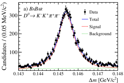
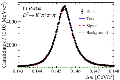
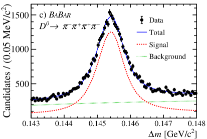
Figure 1: Projections of the unbinned maximum-likelihood fits to the final candidate distributions as a function of $\Delta m$ for the normalization modes in the range $0.143<{\Delta m}<0.148{\mathrm{\,Ge\kern-1.00006ptV\!/}c^{2}}$. The solid blue line is the total fit, the dashed red line is the signal and the dotted green line is the background.

After the application of the selection criteria, there are on the order of 100 events or fewer available for fitting in each signal mode. Each signal mode yield $N_{\rm sig}$ is therefore extracted by performing a one-dimensional unbinned maximum likelihood fit to $\Delta m$ in the range $0.1395<{\Delta m}<0.1610{\mathrm{\,Ge\kern-1.00006ptV\!/}c^{2}}$. A Cruijff function is implemented for the signal mode PDF, except for ${{D}^{0}}\rightarrow\phi\,e^{\pm}\mu^{\mp}$, for which two two-piece Gaussians functions are used, and ${{D}^{0}}\rightarrow{{\rho}^{0}}e^{\pm}\mu^{\mp}$, for which two Cruijff functions are used. The background is modeled with an ARGUS function with the same end point used for the normalization modes. The signal PDF parameters and the end point parameter are fixed in the fit. All other background parameters and the signal and background yields are allowed to vary. Figure 2 shows the results of the fits to the $\Delta m$ distributions for the signal modes.

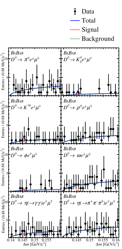
Figure 2: Unbinned maximum-likelihood fits to the final candidate distributions as a function of $\Delta m$ for the signal modes in the range $0.1395<{\Delta m}<0.1610{\mathrm{\,Ge\kern-1.00006ptV\!/}c^{2}}$. The solid blue line is the total fit, the dashed red line is the signal and the dotted green line is the background.

We test the performance of the maximum likelihood fit for the normalization modes by generating ensembles of MC samples from the normalization and background PDF distributions. The mean numbers of normalization and background candidates used in the ensembles are taken from the fits to the data. The numbers of generated background and normalization mode candidates are sampled from a Poisson distribution. All background and normalization mode PDF parameters are allowed to vary, except for the ARGUS function end point. No significant biases are observed in the fitted yields of the normalization modes. The same procedure is repeated for the maximum likelihood fits to the signal modes, with ensembles of MC samples generated from the background PDF distributions only, assuming a signal yield of zero. The signal PDF parameters are fixed to the values used for the fits to the data, and the signal yield is allowed to vary. The biases in the fitted signal yields are less than $\pm 0.3$ candidates for all modes, and these are subtracted from the fitted yields before calculating the signal branching fractions.

To confirm the normalization procedure, the signal modes in Eq. (1) are replaced with the decay ${{D}^{0}}\rightarrow{{K}^{-}}{{\pi}^{+}}$, which has a well-measured branching fraction Tanabashi et al. (2018). The ${{D}^{0}}\rightarrow{{K}^{-}}{{\pi}^{+}}$ decays are reconstructed using the on-peak data sample only ($424.3\pm 1.8$$\mbox{\,fb}^{-1}$). The ${{D}^{0}}\rightarrow{{K}^{-}}{{\pi}^{+}}$ decay is selected using the same criteria as used for the ${{D}^{0}}\rightarrow{{K}^{-}}{{\pi}^{+}}{{\pi}^{+}}{{\pi}^{-}}$ mode, which is used as the normalization mode for this test. The ${{D}^{0}}\rightarrow{{K}^{-}}{{\pi}^{+}}$ signal yield is $1\,881\,950\pm 1380$ with $\epsilon_{\rm sig}=(27.4\pm 0.2)\%$. Thus, we determine ${\mathcal{B}}({{D}^{0}}\rightarrow{{K}^{-}}{{\pi}^{+}})=(3.98\pm 0.08\pm 0.10)$%, where the uncertainties are statistical and systematic, respectively. This is consistent with the current world average of $(3.95\pm 0.03)$% Tanabashi et al. (2018). When the test is repeated using either ${{D}^{0}}\rightarrow{{K}^{-}}{{K}^{+}}{{\pi}^{+}}{{\pi}^{-}}$ or ${{D}^{0}}\rightarrow{{\pi}^{-}}{{\pi}^{+}}{{\pi}^{+}}{{\pi}^{-}}$ as the normalization mode, ${\mathcal{B}}({{D}^{0}}\rightarrow{{K}^{-}}{{\pi}^{+}})$ is determined to be $(3.51\pm 0.18\pm 0.18)\%$ and $(4.12\pm 0.13\pm 0.16)\%$, respectively.

V Systematic Uncertainties

The systematic uncertainties in the branching fraction determinations of the signal modes arise from so-called additive systematic uncertainties that affect the significance of the signal mode yields in the fits to the data samples and from multiplicative systematic uncertainties on the luminosity and signal reconstruction efficiencies.

The main sources of the additive systematic uncertainties in the signal yields are associated with the model parametrizations used in the fits to the signal modes, the fit biases, the allowed invariant-mass ranges for the ${D}^{0}$ and $X^{0}$ candidates, the amount of cross feed, and the limited MC and data sample sizes available for the optimization of the BDT discriminants.

The uncertainties associated with the fit model parametrizations of the signal modes are estimated by repeating the fits with alternative PDFs. This involves replacing the Cruijff functions with Crystal Ball functions, using a two-piece Gaussian function, and changing the number of functions used in the PDFs. For the background, the ARGUS function is replaced by a first- or second-order polynomial. The largest deviation occurs when using the Crystal Ball functions for the signal and the first-order polynomial for the background. The systematic uncertainty is taken as half this maximum deviation. The largest contribution comes from the normalization mode ${{D}^{0}}\rightarrow{{\pi}^{-}}{{\pi}^{+}}{{\pi}^{+}}{{\pi}^{-}}$ due to the presence of increased background and greater uncertainty in the background shape. To account for potential inaccuracies in the simulation of the ${D}^{0}$ and $X^{0}$ invariant mass distributions, we change the mass selection ranges by $\pm 0.5\sigma$, where $\sigma$ is the RMS width of the ${D}^{0}$ or $X^{0}$ meson.

The systematic uncertainties in the correction on the fit biases for the signal yields are taken from the ensembles of fits to the MC samples. Given the central value of the signal yield obtained from the fit in each mode, the cross feed yields from all other modes are calculated and are taken as a systematic uncertainty. To evaluate the systematic uncertainty in the application of the BDT discriminant, we vary the value of the selection criterion for the BDT discriminant output, change the size of the hidden region in data, and also retrain the BDT discriminant using a training sample with a different ensemble of MC samples. Summing the uncertainties in quadrature, the total additive systematic uncertainties in the signal yields are between 0.4 and 0.9 events.

Multiplicative systematic uncertainties are due to assumptions made about the distributions of the final-state particles in the signal simulation modeling, the model parametrizations used in the fits to the normalization modes, the normalization mode branching fractions, tracking and PID efficiencies, limited simulation sample sizes, and luminosity.

Since the decay mechanism of the signal modes is unknown, we vary the angular distributions of the simulated final-state particles from the ${D}^{0}$ signal decay in three angular variables, defined following the prescription of Ref. Aubert et al. (2005). We weight the events, which are simulated uniformly in phase space, using combinations of $\sin$, $\cos$, $\sin^{2}$, and $\cos^{2}$ functions of the angular variables. The reconstruction efficiencies calculated from simulation samples as functions of the three angles are constant, within the statistics available. The deviations of the reweighted efficiencies from the default average reconstruction efficiencies are therefore small. Half the maximum change in the average reconstruction efficiency is assigned as a systematic uncertainty.

Uncertainties associated with the fit model parametrizations of the normalization modes are estimated by repeating the fits with alternative PDFs. This involves swapping the Cruijff and Crystal Ball functions used in both $\Delta m$ and $m({{D}^{0}})$. For the background, the order of the polynomials is changed and the ARGUS function is replaced by a second-order polynomial. Half the maximum change in the fitted yield is assigned as a systematic uncertainty. The normalization modes branching fraction uncertainties are taken from Ref. Tanabashi et al. (2018).

For both signal and normalization modes, we include uncertainties to account for discrepancies between reconstruction efficiencies calculated from simulation and data samples of 1.0% per ${K}^{0}_{\mathrm{\scriptscriptstyle S}}$, 0.8% per lepton, and 0.7% per hadron track Allmendinger et al. (2013). We include a momentum-dependent ${\pi}^{0}$ reconstruction efficiency uncertainty of 2.1% for ${{D}^{0}}\rightarrow{{\pi}^{0}}e^{\pm}\mu^{\mp}$ and 2.3% for ${{D}^{0}}\rightarrow\omega e^{\pm}\mu^{\mp}$ and ${{D}^{0}}\rightarrow\eta(\rightarrow{{\pi}^{+}}{{\pi}^{-}}{{\pi}^{0}})e^{\pm}\mu^{\mp}$. For the PID efficiencies, we assign an uncertainty of 0.7% per track for electrons, 1.0% for muons, 0.2% for charged pions, and 1.1% for kaons Aubert et al. (2013). A systematic uncertainty of 0.4% is associated with our knowledge of the luminosities $\mathcal{L}_{\rm norm}$ and $\mathcal{L}_{\rm sig}$ Lees et al. (2013). We assign systematic uncertainties in the range 0.8% to 1.8% to account for the limited size of the simulation samples available for calculating reconstruction efficiencies for the signal and normalization modes.

The simulation samples for the normalization modes contain a resonant structure of intermediate resonances that decay to two- or three-body final states, as well as four-body nonresonant decays. To investigate how changes in the resonant structure affect the reconstruction efficiencies, the simulation samples were generated using a four-body phase-space distribution only and the reconstruction efficiencies recalculated. The resulting changes in reconstruction efficiencies are less than the statistical uncertainties on $\epsilon_{\rm norm}$ due to the limited size of the simulation samples, and no systematic uncertainties are assigned. The total multiplicative systematic uncertainties are between 4.7% and 6.8% for the normalization modes and between 4.2% and 7.8% for the signal modes.

Table 2 summarizes the contributions of the systematic uncertainties of the normalization modes to the systematic uncertainties in the signal mode branching fractions, as defined in Eq. (1). Table 3 summarizes the systematic uncertainties in the signal mode yields, excluding those due to the normalization modes.

Table 2: Summary of the contributions to the systematic uncertainties on the signal mode branching fractions, as defined in Eq. (1), that arise from uncertainties in the measurement of the normalization modes.

	${{\pi}^{-}}{{\pi}^{+}}{{\pi}^{+}}{{\pi}^{-}}$	${{K}^{-}}{{\pi}^{+}}{{\pi}^{+}}{{\pi}^{-}}$	${{K}^{-}}{{K}^{+}}{{\pi}^{+}}{{\pi}^{-}}$
PDF variation	4.6%	1.0%	1.0%
${K}^{0}_{\mathrm{\scriptscriptstyle S}}$ correction	1.0%	1.0%	1.0%
Tracking correction	3.5%	3.5%	3.5%
PID correction	0.8%	1.7%	2.6%
Luminosity	0.4%	0.4%	0.4%
Normalization $\mathcal{B}$	3.0%	1.8%	4.5%
Simulation size	1.0%	1.0%	0.8%
Total	$6.8$%	$4.7$%	$6.6$%

Table 3: Summary of ${{D}^{0}}\rightarrow X^{0}e^{\pm}\mu^{\mp}$ additive and multiplicative systematic uncertainties, excluding those due to the normalization modes given in Table 2.

$X^{0}=$	${\pi}^{0}$	${K}^{0}_{\mathrm{\scriptscriptstyle S}}$	${\kern 1.99997pt\overline{\kern-1.99997ptK}{}}{}^{*0}$	${\rho}^{0}$	$\phi$	$\omega$	$\eta$	$\eta$
$X^{0}\rightarrow$	$\gamma\gamma$	${{\pi}^{+}}{{\pi}^{-}}$	${{K}^{-}}{{\pi}^{+}}$	${{\pi}^{+}}{{\pi}^{-}}$	${{K}^{+}}{{K}^{-}}$	${{\pi}^{+}}{{\pi}^{-}}{{\pi}^{0}}$	$\gamma\gamma$	${{\pi}^{+}}{{\pi}^{-}}{{\pi}^{0}}$
Additive (events):
PDF variation	0.23	0.05	0.20	0.16	0.17	0.26	0.43	0.16
Fit bias	0.09	0.28	0.21	0.15	0.24	0.09	0.08	0.07
${D}^{0}$/$X^{0}$ mass	0.30	0.04	0.05	0.07	0.07	0.07	0.04	0.23
BDT discriminant	0.83	0.68	0.71	0.30	0.06	0.35	0.27	0.58
Cross feed				0.01			0.06
Subtotal (candidates)	0.92	0.74	0.76	0.38	0.31	0.45	0.52	0.65
Multiplicative (%):
Angular variation	1.4	2.8	2.0	3.4	5.3	1.9	1.6	1.6
${\mathcal{B}}(X^{0})$ subdecay		0.1			1.0	0.8	0.5	1.2
${K}^{0}_{\mathrm{\scriptscriptstyle S}}$ correction		1.0
Tracking correction	2.3	3.7	3.7	3.7	3.7	3.7	2.3	3.7
PID correction	2.7	2.1	3.0	2.1	3.9	3.1	2.7	3.1
${\pi}^{0}$ correction	2.1					2.3		2.3
Luminosity	0.4	0.4	0.4	0.4	0.4	0.4	0.4	0.4
Simulation sample size	1.4	1.3	1.5	1.3	1.4	1.8	1.3	1.5
Subtotal (%)	4.2	5.4	5.4	5.6	7.8	5.7	4.2	5.6

VI Results

Table 4 gives the fitted signal yields, reconstruction efficiencies, branching fractions with statistical and systematic uncertainties, 90% C.L. upper limits on the branching fractions, and previous upper limits Freyberger et al. (1996); Aitala et al. (2001); Tanabashi et al. (2018) for the signal modes. The yields for all the signal modes are compatible with zero. We assume that there are no cancellations due to correlations in the systematic uncertainties in the numerator and denominator of Eq. (1). We use the frequentist approach of Feldman and Cousins Feldman and Cousins (1998) to determine 90% C.L. bands. When computing the limits, the systematic uncertainties are combined in quadrature with the statistical uncertainties in the fitted signal yields.

Table 4: Summary of fitted signal yields $N_{\rm sig}$ with statistical and systematic uncertainties, reconstruction efficiencies $\epsilon_{\rm sig}$, branching fractions with statistical and systematic uncertainties, 90% C.L. upper limits (U.L.) on the branching fractions, and previous limits Freyberger et al. (1996); Aitala et al. (2001); Tanabashi et al. (2018). The additive and multiplicative uncertainties are combined to obtain the overall systematic uncertainties. The branching fraction systematic uncertainties include the uncertainties in the normalization mode branching fractions.

	$N_{\rm sig}$		$\epsilon_{\rm sig}$	$\mathcal{B}$ $(\times 10^{-7})$	$\mathcal{B}$ 90% U.L. $(\times 10^{-7})$
Decay mode	(candidates)		(%)		BABAR	Previous
${{D}^{0}}\rightarrow{{\pi}^{0}}e^{\pm}\mu^{\mp}$	$-0.3\pm 2.0\pm 0.9$		$2.15\pm 0.03$	$-0.6\pm 4.8\pm 2.3$	$8.0$	860
${{D}^{0}}\rightarrow{{K}^{0}_{\mathrm{\scriptscriptstyle S}}}e^{\pm}\mu^{\mp}$	$0.7\pm 1.7\pm 0.7$		$3.01\pm 0.04$	$1.9\pm 4.6\pm 1.9$	$8.6$	500
${{D}^{0}}\rightarrow{{\kern 1.99997pt\overline{\kern-1.99997ptK}{}}{}^{*0}}e^{\pm}\mu^{\mp}$	$0.8\pm 1.8\pm 0.8$		$2.31\pm 0.03$	$2.8\pm 6.1\pm 2.6$	$12.4$	830
${{D}^{0}}\rightarrow{{\rho}^{0}}e^{\pm}\mu^{\mp}$	$-0.7\pm 1.7\pm 0.4$		$2.10\pm 0.03$	$-1.8\pm 4.4\pm 1.0$	$5.0$	490
${{D}^{0}}\rightarrow\phi\,e^{\pm}\mu^{\mp}$	$0.0\pm 1.4\pm 0.3$		$3.43\pm 0.04$	$0.1\pm 3.8\pm 0.9$	$5.1$	340
${{D}^{0}}\rightarrow\omega e^{\pm}\mu^{\mp}$	$0.4\pm 2.3\pm 0.5$		$1.46\pm 0.03$	$1.8\pm 9.5\pm 1.9$	$17.1$	1200
${{D}^{0}}\rightarrow\eta e^{\pm}\mu^{\mp}$				$6.1\pm 9.7\pm 2.3$	$22.5$	1000
with $\eta\rightarrow\gamma\gamma$	$1.6\pm 2.3\pm 0.5$		$2.96\pm 0.04$	$7.0\pm 10.5\pm 2.4$	$24.0$
with $\eta\rightarrow{{\pi}^{+}}{{\pi}^{-}}{{\pi}^{0}}$	$0.0\pm 2.8\pm 0.7$		$2.46\pm 0.04$	$0.4\pm 25.8\pm 6.0$	$42.8$

In summary, we report 90% C.L. upper limits on the branching fractions for seven lepton-flavor-violating ${{D}^{0}}\rightarrow X^{0}e^{\pm}\mu^{\mp}$ decays. The analysis is based on a sample of ${e^{+}e^{-}}$ annihilation data collected with the BABAR detector, corresponding to an integrated luminosity of $468.2\pm 2.0$$\mbox{\,fb}^{-1}$. The limits are in the range $(5.0-22.5)\times 10^{-7}$ and are between 1 and 2 orders of magnitude more stringent than previous ${{D}^{0}}\rightarrow X^{0}e^{\pm}\mu^{\mp}$ decay results. For the four ${{D}^{0}}\rightarrow X^{0}e^{\pm}\mu^{\mp}$ decays with the same final state as the ${{D}^{0}}\rightarrow h^{\prime-}h^{+}e^{\pm}\mu^{\mp}$ decays reported in Ref. Lees et al. (2020), the limits are 1.5 to 3 times more stringent.

VII Acknowledgments

We are grateful for the extraordinary contributions of our PEP-II colleagues in achieving the excellent luminosity and machine conditions that have made this work possible. The success of this project also relies critically on the expertise and dedication of the computing organizations that support BABAR. The collaborating institutions wish to thank SLAC for its support and the kind hospitality extended to them. This work is supported by the US Department of Energy and National Science Foundation, the Natural Sciences and Engineering Research Council (Canada), the Commissariat à l’Energie Atomique and Institut National de Physique Nucléaire et de Physique des Particules (France), the Bundesministerium für Bildung und Forschung and Deutsche Forschungsgemeinschaft (Germany), the Istituto Nazionale di Fisica Nucleare (Italy), the Foundation for Fundamental Research on Matter (The Netherlands), the Research Council of Norway, the Ministry of Education and Science of the Russian Federation, Ministerio de Economía y Competitividad (Spain), the Science and Technology Facilities Council (United Kingdom), and the Binational Science Foundation (U.S.-Israel). Individuals have received support from the Marie-Curie IEF program (European Union) and the A. P. Sloan Foundation (USA).

References

- Paul et al. (2011) A. Paul, I. I. Bigi, and S. Recksiegel, Phys. Rev. D 83, 114006 (2011).
- Schwartz (1993) A. J. Schwartz, Mod. Phys. Lett. A 08, 967 (1993).
- Guadagnoli and Lane (2015) D. Guadagnoli and K. Lane, Phys. Lett. B 751, 54 (2015).
- de Boer and Hiller (2016) S. de Boer and G. Hiller, Phys. Rev. D 93, 074001 (2016).
- Fajfer and Košnik (2015) S. Fajfer and N. Košnik, Eur. Phys. J. C 75, 567 (2015).
- Atre et al. (2009) A. Atre, T. Han, S. Pascoli, and B. Zhang, J. High Energy Phys. 05, 030 (2009).
- Yuan et al. (2013) H. Yuan, T. Wang, G.-L. Wang, W.-L. Ju, and J.-M. Zhang, J. High Energy Phys. 08, 066 (2013).
- Hai-Rong et al. (2015) D. Hai-Rong, F. Feng, and L. Hai-Bo, Chin. Phys. C 39, 013101 (2015).
- Paul et al. (2014) A. Paul, A. de la Puente, and I. I. Bigi, Phys. Rev. D 90, 014035 (2014).
- Burdman et al. (2002) G. Burdman, E. Golowich, J. A. Hewett, and S. Pakvasa, Phys. Rev. D 66, 014009 (2002).
- Fajfer and Prelovšek (2006) S. Fajfer and S. Prelovšek, Phys. Rev. D 73, 054026 (2006).
- Fajfer et al. (2007) S. Fajfer, N. Košnik, and S. Prelovšek, Phys. Rev. D 76, 074010 (2007).
- Aaij et al. (2016) R. Aaij et al. (LHCb Collaboration), Phys. Lett. B 757, 558 (2016).
- Aaij et al. (2017) R. Aaij et al. (LHCb Collaboration), Phys. Rev. Lett. 119, 181805 (2017).
- Lees et al. (2019) J. P. Lees et al. (BABAR Collaboration), Phys. Rev. Lett. 122, 081802 (2019).
- Cappiello et al. (2013) L. Cappiello, O. Cata, and G. D’Ambrosio, J. High Energy Phys. 04, 135 (2013).
- de Boer and Hiller (2018) S. de Boer and G. Hiller, Phys. Rev. D 98, 035041 (2018).
- Kodama et al. (1995) K. Kodama et al. (E653 Collaboration), Phys. Lett. B 345, 85 (1995).
- Freyberger et al. (1996) A. Freyberger et al. (CLEO Collaboration), Phys. Rev. Lett. 76, 3065 (1996).
- Aitala et al. (2001) E. M. Aitala et al. (E791 Collaboration), Phys. Rev. Lett. 86, 3969 (2001).
- Ablikim et al. (2018) M. Ablikim et al. (BESIII Collaboration), Phys. Rev. D 97, 072015 (2018).
- Lees et al. (2020) J. P. Lees et al. (BABAR Collaboration), Phys. Rev. Lett. 124, 071802 (2020).
- Tanabashi et al. (2018) M. Tanabashi et al. (Particle Data Group), Phys. Rev. D 98, 030001 (2018), and 2019 update.
- Aubert et al. (2002) B. Aubert et al. (BABAR Collaboration), Nucl. Instrum. Methods Phys. Res., Sect. A 479, 1 (2002).
- Aubert et al. (2013) B. Aubert et al. (BABAR Collaboration), Nucl. Instrum. Methods Phys. Res., Sect. A 729, 615 (2013).
- Lees et al. (2013) J. P. Lees et al. (BABAR Collaboration), Nucl. Instrum. Methods Phys. Res., Sect. A 726, 203 (2013).
- Lange (2001) D. J. Lange, Nucl. Instrum. Methods Phys. Res., Sect. A 462, 152 (2001).
- T. Sjöstrand (1994) T. Sjöstrand, Comput. Phys. Commun. 82, 74 (1994).
- Ward et al. (2003) B. F. L. Ward, S. Jadach, and Z. Was, Nucl. Phys. Proc. Suppl. 116, 73 (2003).
- H. Czyz and J. H. Kühn (2001) H. Czyz and J. H. Kühn, Eur. Phys. J. C 18, 497 (2001).
- Davidson et al. (2012) N. Davidson, G. Nanava, T. Przedzinski, E. Richter-Was, and Z. Was, Comput. Phys. Commun. 183, 821 (2012).
- Golonka and Was (2006) P. Golonka and Z. Was, Eur. Phys. J. C 45, 97 (2006).
- Agostinelli et al. (2003) S. Agostinelli et al. (GEANT 4 Collaboration), Nucl. Instrum. Methods Phys. Res., Sect. A 506, 250 (2003).
- Allison et al. (2006) J. Allison, K. Amako, J. Apostolakis, H. Araujo, P. Dubois, et al. (GEANT 4 Collaboration), IEEE Trans. Nucl. Sci. 53, 270 (2006).
- Bevan et al. (2014) A. J. Bevan et al. (BABAR and Belle Collaborations), Eur. Phys. J. C 74, 3026 (2014).
- Hulsbergen (2005) W. D. Hulsbergen, Nucl. Instrum. Methods Phys. Res., Sect. A 552, 566 (2005).
- Aubert et al. (2004) B. Aubert et al. (BABAR Collaboration), Phys. Rev. D 69, 111104 (2004).
- Freund and Schapire (1997) Y. Freund and R. E. Schapire, J. Comput. Syst. Sci. 55, 119 (1997).
- Lees et al. (2014) J. P. Lees et al. (BABAR Collaboration), Phys. Rev. D 89, 011102 (2014).
- (40) T. Skwarnicki, A study of the radiative cascade transitions between the and resonances, Ph.D. thesis, Institute of Nuclear Physics, Krakow, DESY-F31-86-02, 1986.
- Albrecht et al. (1990) H. Albrecht et al. (ARGUS Collaboration), Phys. Lett. B 241, 278 (1990).
- Aubert et al. (2005) B. Aubert et al. (BABAR Collaboration), Phys. Rev. D 71, 032005 (2005).
- Allmendinger et al. (2013) T. Allmendinger et al., Nucl. Instrum. Methods Phys. Res., Sect. A 704, 44 (2013).
- Feldman and Cousins (1998) G. J. Feldman and R. D. Cousins, Phys. Rev. D 57, 3873 (1998).