Microrheological approach for the viscoelastic response of gels

Abstract

In this paper I present a simple and self-consistent framework based on microrheology that allows one to obtain the mechanical response of viscoelastic fluids and gels from the motion of probe particles immersed on it. By considering a non-markovian Langevin equation, I obtain general expressions for the mean-squared displacement and the time-dependent diffusion coefficient that are directly related to the memory kernels and the response function, and which allow one to obtain estimates for the complex shear modulus and the complex viscosity of the material. The usefulness of such approach is demonstrated by applying it to describe experimental data on chemically cross-linked polyacrylamide through its sol-gel transition.

I Introduction

Gelatin is one of those curious materials that call attention of any children, as it happened with the young James Clerk Maxwell Campbell and Garnett (1882), who later put forward one of the first descriptions of what we known as viscoelasticity Maxwell (1877). Constitutive equations, like those defined by Maxwell’s and Kelvin-Voigt’s models Ferry (1980); Larson (1999), are the basis of many theoretical approaches that are still used today to describe the relaxation modulus $G(t)$ and the compliance $J(t)$ of viscoelastic materials. In fact, the mechanical response of gels can be more complicated and usually one resort to generalized models which assume that $G(t)$ can be evaluated from a relaxation time distribution $H(\lambda)$, also known as relaxation spectrum Ferry (1980); Mours and Winter (2000), that is

$$G(t)=G_{0}+\int_{0}^{\tau_{c}}H(\lambda)\frac{e^{-t/\lambda}}{\lambda}d\lambda~{}~{},$$ (1)

where $\lambda$ denotes the relaxation times below a cutoff value $\tau_{c}$ and $G_{0}$ corresponds to a discrete infinite-time contribution for the shear modulus.

The basic idea is that $H(\lambda)$ should include informations about all the microscopic and mesoscopic structures of the gel Mours and Winter (2000), and that would provide some reasoning on what is been observed in the complex shear modulus, $G^{*}(\omega)=G^{\prime}(\omega)+iG^{\prime\prime}(\omega)$. The storage, $G^{\prime}(\omega)$, and the loss, $G^{\prime\prime}(\omega)$, moduli are the main rheological properties measured in oscillatory sweeping experiments Larson (1999) and can be obtained from $G(t)$ through a Fourier transform Doi (2015). In particular, when the gel network is not formed yet, one have that $G_{0}=0\,$Pa and both $G^{\prime}(\omega)$ and $G^{\prime\prime}(\omega)$ goes to zero at low frequencies, and that is a characteristic behavior of liquid-like solutions. On the other hand, the material will behave like a semisolid Rao (2014) if the storage modulus of a gel is given by $G^{\prime}(\omega)=G_{0}$ at low frequencies, and that is usually interpreted in terms of the formation of a network. Unfortunately, the evaluation the complex modulus $G^{*}(\omega)$ from $H(\lambda)$ is not a trivial task and in the most of cases it is done only numerically Ferry (1980); Mours and Winter (2000).

Although several descriptions of gelation are possible Zaccarelli (2007), most of the successful theoretical developments were based on the analogy between percolation and the sol-gel transition Flory (1953); de Gennes (1979); Rubinstein and Colby (2003), including the pioneering works done by Flory Flory (1941) and Stockmayer Stockmayer (1943). Fractality was a concept that emerged naturally from the percolation analogy, and Ref. Martin and Adolf (1991) present a review on that topic, including complementary approaches that are based on the aggregation kinetics. For example, in a recent study presented in Ref. Zaccone et al. (2014), the authors established an interesting link between the growth kinetics mechanisms and the viscoelastic response of the solution by assuming that the relaxation times of the gels structures are related to the size of the clusters in solution. Their approach lead to a semi-empirical expression for the relaxation spectrum, i.e., $H(\lambda)\propto\lambda^{-q}\exp[-(\lambda/\tau_{c})^{w}]$, with the exponents $q$ and $w$ related to the fractal dimension of the clusters, and that was used with Eq. 1 to estimate the shear moduli of the colloidal suspensions Zaccone et al. (2014).

Fractal properties of gels are usually probed by light scattering experiments and, in terms of dynamics, it is worth mentioning the work of Krall and co-workers Krall, Huang, and Weitz (1997); Krall and Weitz (1998), which have related the measurements of the dynamic structure factor $f(q,t)$ to an expression for the mean-squared displacement of the fractal structures present in colloidal gels. Importantly, they found a function $f(q,t)$ that decays to a finite plateau at long times, and interpreted that in terms of a finite elastic modulus $G_{0}$.

A coupled of years before, Mason and Weitz Mason and Weitz (1995), which are considered the founders of microrheology Waigh (2005, 2016), established a generalized Stokes-Einstein relationship (GSER) and, by exploring light scattering experiments as well, demonstrate that one can extract the complex modulus $G^{*}(\omega)$ of colloidal systems from the mean-squared displacement (MSD) $\langle\Delta r^{2}(t)\rangle$ of probe particles. At the linear viscoelastic (LVE) response regime Rizzi and Tassieri , one can use such GSER to estimate the compliance $J(t)$ of the viscoelastic material from the MSD of probe particles immersed on it as Squires and Mason (2010)

$$J(t)=\frac{3\pi a}{dk_{B}T}\langle\Delta r^{2}(t)\rangle~{}~{},$$ (2)

where $a$ is the radius of the probe particles, $k_{B}$ and $T$ are the Boltzmann’s constant and the absolute temperature, respectively, and $d$ is the number of degrees of freedom of the random walk (e.g., $d=3$ for diffusing wave spectroscopy, and $d=2$ for particle tracking videomicroscopy Waigh (2016); Rizzi and Tassieri ).

There are a few exact interrelations between the rheological functions Ferry (1980), e.g., between the complex modulus and the complex viscosity, $G^{*}(\omega)=i\omega\,\eta^{*}(\omega)$, and one can conveniently use Eq. 2 to evaluate the complex shear modulus by considering Rizzi and Tassieri

$$G^{*}(\omega)=\frac{1}{i\omega\hat{J}(\omega)}~{}~{},$$ (3)

where $\hat{J}(\omega)$ is the Fourier transform of the compliance $J(t)$, which might be evaluated exactly through a Fourier-Laplace integral, or numerically by the method proposed in Ref. Evans et al. (2009). Equations 2 and 3 opened the way for many techniques that were used to measure the MSD of probe particles to be applied in the characterization of viscoelastic materials Rizzi and Tassieri . In particular, there are several studies in the literature that use particle tracking microrheology to obtain the compliance and shear moduli of protein systems during the gelation transition Larsen and Furst (2008); Larsen, Schultz, and Furst (2008); Corrigan and Donald (2009a, b); Aufderhorst-Roberts et al. (2014).

In this paper I consider an approach based on Langevin dynamics to derive general expressions for the MSD $\langle\Delta r^{2}(t)\rangle$ and the time-dependent diffusion coefficient $D(t)$ of particles immersed in a viscoelastic material described by effective elastic and friction constants. I provide explicity expressions that link the MSD to the response and memory functions and discuss how such Langevin equation is related to a Fokker-Planck type of equation. By using a microrheological approach based on Eqs. 2 and 3, I obtain the complex shear moduli $G^{*}(\omega)$ and the complex viscosity $\eta^{*}(\omega)$ of the material, and show how such rheological properties are connected to the effective constants defined in the Langevin equation. I validate my approach by considering experimental data on the sol-gel transition of chemically cross-linked polyacrylamide gels Larsen and Furst (2008), and demonstrate that the expression for the MSD used to describe the dynamics of probe particles in a gel phase of fibrillar proteins Rizzi (2017) can be also used to describe their dynamics in the sol phase.

II Microrheological approach

II.1 Langevin equation

First, consider that the motion of probe particles immersed in a viscoelastic material can be described by an overdamped Langevin equation that is given by

$$\zeta\frac{d\vec{r}}{dt}=-\kappa\int_{0}^{t}dt^{\prime}b(t-t^{\prime})\vec{r}(t^{\prime})+\vec{f}(t)~{}~{},$$ (4)

where $\zeta$ and $\kappa$ are the effective friction coefficient and the effective elastic constant of the material, respectively; $b(t-t^{\prime})$ is a memory kernel function which indicates that the particle is submitted to a non-markovian harmonic-like potential; $\vec{f}(t)$ is a random force with gaussian statistical properties such that $\langle\vec{f}\,\rangle=\vec{0}\,$, and

$$\langle\vec{f}(t)\cdot\vec{f}(t^{\prime})\rangle=dk_{B}T\,\zeta\,b(t-t^{\prime})~{}~{}.$$ (5)

In order to obtain a general expression for the mean-squared displacement of the probe particles, one can apply the Laplace transform, here denoted by $\tilde{z}(t)=\mathcal{L}[\vec{z}(t);s]=\int_{0}^{\infty}\vec{z}(t)\,e^{-st}dt$, to both sides of Eq. 4, which leads to

$$\tilde{r}(s)=\bar{\chi}(s)[\vec{r}(0)+\zeta^{-1}\tilde{f}(s)]~{}~{},$$ (6)

where

$$\bar{\chi}(s)=\frac{1}{s+(\kappa/\zeta)\bar{b}(s)}~{}~{},$$ (7)

with $\bar{b}(s)=\mathcal{L}[b(t);s]$. Hence, the general solution of Eq. 4 is given by

$$\vec{r}(t)=\chi(t)\vec{r}(0)+\zeta^{-1}\int_{0}^{t}\chi(t-t^{\prime})\vec{f}(t^{\prime})dt^{\prime}~{}~{},$$ (8)

where $\chi(t)$ is a response function related to the memory kernel $b(t)$ through $\chi(t)=\mathcal{L}^{-1}\{[s+(\kappa/\zeta)\bar{b}(s)]^{-1};t\}$ (see Eq. 7). Now, following Ref. Adelman (1976), one can define

$$\vec{y}(t)=\vec{r}(t)-\chi(t)\vec{r}(0)=\zeta^{-1}\int_{0}^{t}\chi(t-t^{\prime})\vec{f}(t^{\prime})dt^{\prime}$$ (9)

and, by considering Eq. 5, evaluate the fluctuation function of $\vec{y}(t)$, i.e., $A(t)=\langle\vec{y}(t)\cdot\vec{y}(t)\rangle$, which is given by

$$A(t)=\frac{dk_{B}T}{\zeta}\int_{0}^{t}\int_{0}^{t}\chi(t-t^{\prime})b(t^{\prime}-t^{\prime\prime})\chi(t-t^{\prime\prime})dt^{\prime}dt^{\prime\prime}~{}~{}.$$ (10)

Also, one should compute its time derivative,

$$\frac{\partial A(t)}{\partial t}=\frac{2dk_{B}T}{\zeta}\chi(t)\int_{0}^{t}b(t-t^{\prime})\chi(t^{\prime})dt^{\prime}~{}~{}.$$ (11)

Now, from Eq. 7 one have that

$$s\bar{\chi}(s)-1=-\frac{\kappa}{\zeta}\bar{b}(s)\bar{\chi}(s)~{}~{},$$ (12)

and, since Eq. 8 requires that $\chi(0)=1$, the inverse Laplace transform of Eq. 12 will be given by

$$-\frac{\zeta}{\kappa}\frac{\partial\chi(t)}{\partial t}=\mathcal{L}^{-1}[\bar{b}(s)\bar{\chi}(s);t]=\int_{0}^{t}b(t-t^{\prime})\chi(t^{\prime})dt^{\prime}~{}~{},$$ (13)

so that Eq. 11 can be rewritten as

$$\frac{\partial A(t)}{\partial t}=-\frac{2dk_{B}T}{\kappa}\chi(t)\frac{\partial\chi(t)}{\partial t}~{}~{}.$$ (14)

Thus, from the above equation one can infer that the fluctuation function defined by Eq. 10 should be given by

$$A(t)=\frac{dk_{B}T}{\kappa}\left[1-\chi^{2}(t)\right]~{}~{},$$ (15)

from where one can obtain the mean-squared displacement, $\langle\Delta r^{2}(t)\rangle\equiv A(t)$, by choosing, without loss of generality, $\vec{r}(0)=\vec{0}\,$.

II.2 Fokker-Planck equation

Importantly, if the random process defined by Eq. 4 is gaussian, one can assume that the time-dependent position distribution function is given by

$$P(\vec{r},t)\propto\frac{1}{\left[2\pi A(t)\right]^{d/2}}\exp\left\{-\frac{[\vec{r}(t)]^{2}}{2A(t)}\right\}~{}~{},$$ (16)

which corresponds to the solution of a Fokker-Planck type of equation that is characteristic of non-markovian processes and can be written as Adelman (1976)

$$\frac{\partial P(\vec{r},t)}{\partial t}=k_{B}T\beta(t)\nabla_{r}\left[\nabla_{r}P(\vec{r},t)+P(\vec{r},t)\left(\frac{\kappa\vec{r}}{k_{B}T}\right)\right]~{},$$ (17)

where $\beta(t)$ is a memory function defined as

$$\beta(t)=-\frac{1}{\kappa}\frac{1}{\chi(t)}\frac{\partial\chi(t)}{\partial t}~{}~{}.$$ (18)

Interestingly, from Eqs. 13 and 18 one finds that

$$\beta(t)\,\chi(t)=\frac{1}{\zeta}\int_{0}^{t}b(t-t^{\prime})\chi(t^{\prime})dt^{\prime}~{}~{},$$ (19)

which indicates that, in general, there is no simple relationship between the memory kernel $b(t)$ defined in Eq. 4 and the functions $\chi(t)$ and $\beta(t)$. In particular, one can observe that the memory function $\beta(t)$ should be related, but it is not generally equal, to the mobility function $\mu(t)=(2dk_{B}T)^{-1}(\partial A(t)/\partial t)$, which can be evaluated from Eqs. 14 and 18 as

$$\mu(t)=\beta(t)\,\chi^{2}(t)~{}~{}.$$ (20)

II.3 Alternative Langevin equation

It is worth mentioning that the aforementioned Langevin approach defined by Eq. 4 can be written in terms of an alternative Langevin equation, where the effective elastic force is equivalent to a delayed viscous force, that is

$$\kappa\vec{r}(t)=-\zeta\int_{0}^{t}u(t-t^{\prime})\vec{v}(t^{\prime})dt^{\prime}+\vec{g}(t)$$ (21)

with $\langle\vec{g}(t)\,\rangle=\vec{0}$ and $\langle\vec{g}(t)\cdot\vec{g}(t^{\prime})\rangle=dk_{B}T\,\kappa\,u(t-t^{\prime})$. One can show that the Laplace transform of Eq. 21 yields

$$\tilde{r}(s)=\left[s+\frac{(\kappa/\zeta)}{\bar{u}(s)}\right]^{-1}\left[\vec{r}(0)+\zeta^{-1}\frac{\tilde{g}(s)}{\bar{u}(s)}\right]~{}~{}.$$ (22)

Thus, by directly comparing Eqs. 6 and 22, and identifying the first multiplying term in the above equation as $\bar{\chi}(s)$ defined by Eq. 7, one can verify that the two Langevin equations will be equivalent when $\tilde{g}(s)=\bar{u}(s)\tilde{f}(s)$, and

$$\bar{u}(s)\,\bar{b}(s)=1~{}~{}.$$ (23)

Interestingly, a similar result was found in Refs. Panja (2010a, b), where the author obtain approximate expressions for the memory kernels of a tagged particle attached by springs to the middle of a Rouse polymeric chain.

Once that the two approaches are equivalent, the same reasoning presented in Sec. II.2 should be valid. In particular, by considering Eqs. 12 and 23, one finds that

$$\chi(t)=-\frac{\zeta}{\kappa}\int_{0}^{t}u(t-t^{\prime})\dot{\chi}(t^{\prime})dt^{\prime}~{}~{},$$ (24)

which is complementary to Eq. 19.

II.4 Mean-squared displacement (MSD)

Importantly, Eq. 18 sets a differential equation for $\chi(t)$, which one can assume that have a solution that is given by

$$\chi(t)=\chi(0)\,e^{-\kappa\psi(t)}~{}~{},$$ (25)

from where one can identify $\beta(t)=\partial\psi(t)/\partial t$, or $\psi(t)=\int_{0}^{t}\beta(t^{\prime})dt^{\prime}$, with

$$\psi(t)=\frac{1}{\kappa}\ln\left[\frac{\chi(0)}{\chi(t)}\right]~{}~{}.$$ (26)

Thus, the MSD can be computed from Eqs. 15 and 25 as

$$\langle\Delta r^{2}(t)\rangle=\frac{dk_{B}T}{\kappa}\left[1-e^{-2\kappa\psi(t)}\right]~{}~{}.$$ (27)

In principle, such expression for the MSD can be also derived from the Fokker-Planck equation, Eq. 17, e.g., by considering the time derivative of $\langle\vec{r}^{\,2}(t)\rangle=\int P(\vec{r},t)r^{2}dr$ with $P(\vec{r},t)$ given by Eq. 16 (see, e.g., Ref. Sarmiento-Gomez, Santamaría-Holek, and Castillo (2014)).

In addition, one can evaluate the time-dependent diffusion coefficient as the time derivative of the MSD, that is, $D(t)=(2d)^{-1}\partial\langle\Delta r^{2}(t)\rangle/\partial t$, which yields

$$D(t)=k_{B}T\mu(t)~{}~{},$$ (28)

with the mobility $\mu(t)$ computed by Eq. 20.

II.5 Examples

In this Section, I include four paradigmatic examples that are discussed in terms of the aforementioned framework and which will be useful to the following theoretical developments.

II.5.1 Simple viscoelastic medium

The most trivial example corresponds to the case where the probe particle is subjected to a harmonic potential described by a markovian process so that the memory kernel in Eq. 4 is given by a delta function, i.e., $b(t)=\delta(t)$, then $\beta=1/\zeta$ follows from Eq. 19, and $\psi(t)=\int_{0}^{t}\beta(t^{\prime})dt^{\prime}=t/\zeta$, hence Eq. 25 gives $\chi(t)=e^{-\kappa t/\zeta}$. In this case, the MSD obtained by Eq. 27 can be used to evaluate the compliance through Eq. 2, which yields $J(t)=(3\pi a/\kappa)[1-\exp(-2t/\tau)]$, from where one can identify $\tau=\zeta/\kappa$ as a characteristic relaxation time. As shown in Ref. Azevedo and Rizzi (2020), one can plug $J(t)$ into Eq. 3 to obtain the storage modulus, $G^{\prime}(\omega)=(\kappa/3\pi a)$, and the loss modulus, $G^{\prime\prime}(\omega)=(\zeta/6\pi a)\omega$, which are the typical response functions observed for a Kelvin-Voigt model Ferry (1980). Also, one can obtain the viscosity $\eta^{\prime}(\omega)=G^{\prime\prime}(\omega)/\omega=(\zeta/6\pi a)$, which is equivalent to the well-known Stokes’ result, $\zeta=6\pi a\eta$.

II.5.2 Normal diffusion in a simple fluid

Another example include the case where the probe particle is immersed in a simple fluid with viscosity $\eta$ and display a normal diffusion behavior. Such regime can be retrieved by choosing a negative value for the elastic constant, $\kappa=-\zeta/(2\tau)$, and $\chi(t)=[(t/\tau)+1]^{1/2}$ (which is similar to set $\chi(t)\approx e^{t/2\tau}$ for $t\ll\tau$), then Eq. 26 yields $\psi(t)=(\tau/\zeta)\ln[(t/\tau)+1]$ and Eq. 18 leads to $\beta(t)=\zeta^{-1}[(t/\tau)+1]^{-1}$. In this case, Eq. 20 yields a constant mobility function, $\mu(t)=1/\zeta$, so that $D(t)=k_{B}T/\zeta$, and Eq. 27 leads to $\langle\Delta r^{2}(t)\rangle=2d(k_{B}T/\zeta)t$. Then, one can use such MSD to obtain the mechanical response of the fluid through Eqs. 2 and 3, that is, $G^{\prime}(\omega)=0$, $G^{\prime\prime}(\omega)=\eta\omega$, and $\eta^{\prime}(\omega)=\eta$. It might be surprising that Eq. 4 could describe a simple fluid by an effective elastic media, however, those results can be also interpreted in terms of the alternative Langevin equation presented in Sec. II.3. By considering Eq. 24, one can check that, in this case, the effective elastic force defined in Eq. 21 should correspond to a delayed viscous force with a kernel function given by $u(t-t^{\prime})=\delta(t-t^{\prime})[(t^{\prime}/\tau)+1]$.

II.5.3 Polymer solutions

In general, the diffusion of probe particles immersed in solutions of polymers are characterized by a subdiffusive behavior with $\langle\Delta r^{2}(t)\rangle\propto t^{n}$ at intermediary times, and a normal diffusion behavior with $\langle\Delta r^{2}(t)\rangle\propto t$, at times longer than the longest relaxation time of the chains Doi and Edwards (1986). The exponent $n$ depends on the kind of polymer considered, e.g., $n=1/2$ for flexible polymeric chains described by the Rouse model, and $n=3/4$ for semiflexible polymers Rubinstein and Colby (2003). Based on Refs. Panja (2010b, a), the dynamics of particles subjected to polymeric chains could be attained, in principle, by considering a kernel function like $u(t)\propto\,t^{-n}e^{-t/\tau}$. Interestingly, the kernel function $u(t)$ for $n=1/2$ presented in Refs. Panja (2010b, a) has the same functional form of the approximated expression found for the relaxation modulus $G(t)$ in Ref. Rubinstein and Colby (2003) when obtaining $G^{*}(\omega)$ for the Rouse chains. In principle, one could compute the Laplace transform of $u(t)$ and consider Eqs. 7 and 23 to obtain $\bar{\chi}(s)$, however, even for such approximated expression, the response function does not have a simple inverse Laplace transform. Anyhow, it is instructive to consider times shorter than $\tau$, where the MSD is given by $\langle\Delta r^{2}(t)\rangle\approx(dk_{B}T/\kappa)(t/\tau)^{n}$, then Eq. 2 yields $J(t)\approx(3\pi a/\kappa)(t/\tau)^{n}$ so that $\tilde{J}(s)=\mathcal{L}[J(t);s]=(3\pi a/\kappa\tau^{n})\Gamma(n+1)/s^{n+1}$, where $\Gamma(n+1)$ is the usual gamma function. Thus, by replacing $s=i\omega$ and using Eq. 3, one finds that $G^{\prime}(\omega)$ and $G^{\prime\prime}(\omega)$ will be both proportional to $\omega^{n}$ at frequencies above $\tau^{-1}$. For instance, $G^{\prime}(\omega)\propto G^{\prime\prime}(\omega)\propto\omega^{1/2}$ for Rouse chains, and $G^{\prime}(\omega)\propto G^{\prime\prime}(\omega)\propto\omega^{3/4}$ for semiflexible chains. As discussed in Ref. Duarte, Teixeira, and Rizzi , solutions with structures of intermediary size and/or flexibility might display intermediary values of $n$.

II.5.4 Polymer network

Finally, it is worth mentioning the widespread expression that have been used in the literature to describe the motion of probe particles in viscoelastic materials, which is given by

$$\langle\Delta r^{2}(t)\rangle=\frac{dk_{B}T}{\kappa}\left[1-e^{-(t/\tau)^{n}}\right]~{}~{}.$$ (29)

To my knowledge, such expression was first derived by Krall and co-workers Krall, Huang, and Weitz (1997); Krall and Weitz (1998) by assuming a fractal structure for the gel network using ideas that are closely related to a description based on percolation theory. Interestingly, one can obtain Eq. 29 from Eq. 27 by choosing $\chi(t)=e^{-(1/2)(t/\tau)^{n}}$, so that Eq. 26 leads to $\psi(t)=(2\kappa)^{-1}(t/\tau)^{n}$ and a memory function given by $\beta(t)=\partial\psi(t)/\partial t=n(2\kappa\tau)^{-1}(t/\tau)^{n-1}$. Unfortunately, as discussed in Ref. Rizzi (2017), the derivative of Eq. 29 does not provide a consistent description between the evaluated $D(t)$ and the time-dependent diffusion coefficient observed in light scattering experiments Teixeira, Geissler, and Licinio (2007); and the MSD given by Eq. 29 does not fit master curves very well Romer et al. (2014); Rizzi (2017). Also, the memory fuction $\beta(t)$ at long times does not decay as $t^{-1}$, so that it is not consistent with fluctuating hydrodynamics theory Adelman (1976). In any case, probably due to its simplicity, such expression have been largely used in the literature (see, e.g., Refs. Romer, Scheffold, and Schurtenberger (2000); Santamaría-Holek and Rubi (2006); Teixeira, Geissler, and Licinio (2007); Romer et al. (2014); Sarmiento-Gomez, Santamaría-Holek, and Castillo (2014); Calzolari et al. (2017)).

III Results

In the following I apply the framework developed in Sec. II in order to obtain self-consistent expressions which can be used to describe the dynamics of probe particles during gelation, hence the viscoelasticity of the material, for both sol and gel phases. Also, I present a comparison with experimental data in order to validate my approach.

III.1 Generalized response function

First, I consider that the viscoelastic material present a local response function which is similar to that discussed in the last example of Sec. II.5, that is, $\chi_{\varepsilon}(t)=e^{-\varepsilon\psi_{\kappa}(t)}$, where $\psi_{\kappa}(t)=\alpha(2\kappa)^{-1}(t/\tau)^{n}$ and $\varepsilon$ is a local effective elastic constant which might depend generally on the local properties of the structures in the viscoelastic material, e.g., cluster/chain sizes in solutions, and mesh sizes/coordination numbers in networks. In this case, the exponent $n$ in $\psi_{\kappa}(t)$ is directly related to a structural dynamic exponent, e.g., $n=1/2$ for Rouse chains and $n=3/4$ for semiflexible polymers Duarte, Teixeira, and Rizzi , and it should characterize the exponent observed at the gelation transition; and $\alpha$ is an exponent that characterizes the distribution of elastic constants $\varepsilon$, which it is assumed to be given by a gamma distribution Crooks (2019), that is

$$\rho_{\alpha}(\varepsilon)=\frac{\alpha^{2}}{4|\kappa|\,\Gamma(1+\alpha/2)}\left(\frac{\alpha}{2\kappa}\varepsilon\right)^{-(1-\alpha/2)}\exp\left(-\frac{\alpha}{2\kappa}\varepsilon\right)~{}~{},$$ (30)

where $\Gamma(1+\alpha/2)$ denotes the usual gamma function. Importantly, Eq. 30 is chosen in order to have the mean value of the local elastic constants $\varepsilon$ consistent with $\bar{\varepsilon}=\kappa$. Also, it is worth mentioning that the effective elastic constants have been related to, e.g., the size of clusters of particles/polymers with a given size Krall, Huang, and Weitz (1997); Dinsmore et al. (2006), and that gamma distributions have been already used to describe size distributions Xue, Homans, and Radford (2009).

Now, by changing the variable to $\xi=(\alpha\varepsilon/2\kappa)$, so that $\chi_{\xi}(t)=e^{-\xi(t/\tau)^{n}}$, one finds that the distribution of effective dimensionless elastic constants, $\xi$, can be written as $\rho_{\alpha}(\xi)=\xi^{-(1-\alpha/2)}e^{-\xi}/\Gamma(\alpha/2)$, so that the effective response function of the viscoelastic material can be evaluated exactly Gradshteyn and Ryzhik (2007), and is given by

$$\chi(t)=\int_{0}^{\infty}\rho_{\alpha}(\xi)\,\chi_{\xi}(t)\,d\xi=\left[\left(\frac{t}{\tau}\right)^{n}+1\right]^{-\alpha/2}~{}~{},$$ (31)

which is valid for $\alpha>-2$, and the mean value of $\xi$ is related to the exponent as $\bar{\xi}=\alpha/2$. Note that, if $\alpha$ is negative, one should also assume that $\kappa<0$, which leads to negative values of $\bar{\xi}$ and $\bar{\varepsilon}$ as well.

Also, by considering Eq. 26, Eq. 31 leads to

$$\psi(t)=\frac{\alpha}{2\kappa}\ln\left[\left(\frac{t}{\tau}\right)^{n}+1\right]~{}~{},$$ (32)

with a memory function $\beta(t)=\partial\psi(t)/\partial t$ given by

$$\beta(t)=\frac{\alpha n}{2\kappa\tau}\left(\frac{t}{\tau}\right)^{n-1}\bigg{/}~{}\left[\left(\frac{t}{\tau}\right)^{n}+1\right]~{}~{},$$ (33)

Figure 1 illustrates the behavior of the functions $\psi(t)$ and $\beta(t)$ that were obtained from the experimental data presented in Fig. 2. Interestingly, both $\psi(t)$ and $\beta(t)$ display positive values and present the same general behavior for both sol and gel phases, even though the sol phase required negative values for $\alpha$ and $\kappa$. At short times, $t\ll\tau$, the logarithm in Eq. 32 can be expanded around 1, so that $\psi(t)\approx(\alpha/2\kappa)(t/\tau)^{n}$ and $\beta(t)\approx(\alpha n/2\kappa\tau)(t/\tau)^{n-1}$. On the other hand, at later times, $t\gg\tau$, one have that $(t/\tau)^{n}+1\approx(t/\tau)^{n}$ so that Eqs. 32 and 33 yield $\psi(t)\approx(\alpha n/2\kappa)\ln(t/\tau)$ and $\beta(t)\approx(\alpha n/2\kappa\tau)(t/\tau)^{-1}$, respectively. Contrary to what is observed for the corresponding memory function $\beta(t)$ evaluated from Eq. 29, the limit of Eq. 33 at long times, i.e., $\beta(t)\propto t^{-1}$, is consistent with fluctuating hydrodynamics theory Adelman (1976), and, accordingly, it does not depend either on $n$ or $\alpha$ (see Fig. 1).

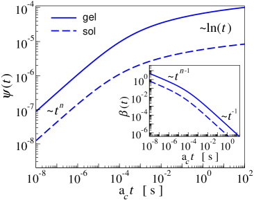
Figure 1: Function $\psi(t)$ (main panel), Eq. 32, and the memory function $\beta(t)$ (inset), Eq. 33, that correspond to the master curves presented in Fig. 2. The dynamics of both sol and gel phases are described by the same exponent $n=0.55$ and those functions display curves with a similar behavior in a log-log plot. For the gel phase one have $\kappa=2.74\times 10^{4}\,$Pa.nm, $\tau=8.63\times 10^{-5}\,$s, and $\alpha=0.71$, so that $\alpha n\approx 0.39$. For the sol phase one have that $\kappa=-8.81\times 10^{5}\,$Pa.nm, $\tau=3\times 10^{-5}\,$s, and $\alpha=-1.8$, so that $-\alpha n\approx 1$.

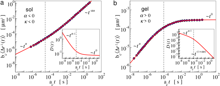
Figure 2: Master curves of the mean-squared displacement illustrating the typical diffusing behaviors observed in (a) sol and (b) gel phases, respectively. All parameters and curves are displayed as rescaled quantities as they were multiplied by factors $\text{a}_{c}$ and/or $\text{b}_{c}$, e.g., MSD $\text{b}_{c}\langle\Delta r^{2}(t)\rangle$, and time $\text{a}_{c}t$, which are experimentally obtained shift factors used to construct the rescaled curves. Filled symbols correpond to the experimental data extracted from Ref. Larsen and Furst (2008) on cross-linked polyacrylamide solutions, while continuous lines denote curves obtained using Eq. 34. Vertical dotted lines indicate the values of characteristic times, $\tau=3\times 10^{-5}\,$s (sol phase) and $\tau=8.63\times 10^{-5}\,$s (gel phase), which separate the subdiffusive behavior with exponent $n=0.55$ at short times from the later time regimes, in which the sol-phase is characterized by the presence of a normal diffusion behavior obtained with $\alpha=-1.8$ so that $-\alpha n\approx 1$, while the limited diffusion observed in the gel-phase is obtained with $\alpha=0.71$. The values of the effective elastic constant are $\kappa=-8.81\times 10^{5}\,$Pa.nm (sol phase) and $\kappa=2.74\times 10^{4}\,$Pa.nm (gel phase). Inset: time-dependent diffusion coefficient $D(t)$ obtained from the corresponding master curves by Eq. 35.

III.2 Probe particle dynamics

Now, by considering the response function given by Eq. 31, one can obtain the expression for the MSD through Eq. 27, which gives,

$$\langle\Delta r^{2}(t)\rangle=\frac{dk_{B}T}{\kappa}\left\{1-\left[\left(\frac{t}{\tau}\right)^{n}+1\right]^{-\alpha}\right\}~{}~{}.$$ (34)

Importantly, such expression can be thought as obtained by averaging the trajectories over many mesoscopic regions of the sample just like in the experiments that use multi-particle techniques Rizzi and Tassieri . Also, it can be considered an alternative to Eq. 29 and, as explored in Ref. Rizzi (2017), it can be used to describe the dynamics of probe particles immersed in viscoelastic materials with a semisolid response like gels Rao (2014). In fact, as I demonstrate below, Eq. 34 is a general expression that can be used to describe the MSD of probe particles immersed in a complex fluid, i.e., in the sol phase, as well.

In addition, one can also evaluate the time-dependent diffusion coefficient $D(t)$ from Eqs. 31 and 33 through Eq. 28, which yields

$$D(t)=k_{B}T\frac{\alpha n}{2\kappa\tau}\left(\frac{t}{\tau}\right)^{n-1}\bigg{/}~{}\left[\left(\frac{t}{\tau}\right)^{n}+1\right]^{1+\alpha}~{}~{}.$$ (35)

It is worth noting that, just as discussed earlier for the functions $\psi(t)$ (Eq. 32) and $\beta(t)$ (Eq. 33), $\alpha$ should adopt the same sign of $\kappa$ in order to have $D(t)$ as a positive-valued function. Also, as expected from Sec. II.2, the long time behavior of the memory function, i.e., $\beta(t)\approx(\alpha n/2\kappa)t^{-1}$, is clearly different from that of Eq. 35 when $t\gg\tau$, that is

$$D(t)\approx k_{B}T\frac{\alpha n}{2\kappa\tau}\left(\frac{t}{\tau}\right)^{-(1+\alpha n)}~{}~{}.$$ (36)

Interestingly, if one defines $\delta(t)=(2d)^{-1}\langle\Delta r^{2}(t)\rangle/t$ with $\langle\Delta r^{2}(t)\rangle$ given by Eq. 34 then, at later times ($t\gg\tau$), $\delta(t)\approx(k_{B}T/2\kappa)t^{-1}$ if $\kappa$ is positive. If $\kappa$ is negative and $\alpha\approx-1/n$, then one obtain basically the same result, i.e., $\delta(t)\approx-(k_{B}T/2\kappa)t^{\alpha n}$, with $\kappa<0$ and $\alpha n\approx-1$.

In order to validate my approach, I include in Fig. 2 results that were obtained from the experimental data taken from Ref. Larsen and Furst (2008), where the authors studied the sol-gel transition of chemically cross-linked polyacrylamide gels. The microrheology experiments were done with the particle tracking videomicroscopy technique ($d=2$) using fluorescent polystyrene microspheres with radius $a=525\,$nm, and I presume that the experiments were done at room temperature, i.e., $T=298\,$K (or $k_{B}T=4.114\,$pN.nm).

The master curves for the MSD were generated from several experiments at different concentrations ($c$ in %wt) of bis-acrylamide cross-linker, and one can recover the actual data by using the shift factors $\text{a}_{c}$ and $\text{b}_{c}$ that are available in Ref. Larsen and Furst (2008). Figure 2(a) displays the typical behavior observed for probe particles immersed in the sol phase, with the long time diffusive behavior being characteristic of a fluid-like solution with $\langle\Delta r^{\,2}(t)\rangle\propto t$ and $D(t)$ independent of time. Figure 2(b) corresponds to a restricted motion of the probe particles, which is tipically observed in the gel phase, with $\langle\Delta r^{\,2}(t)\rangle$ going to a constant value for long times. Indeed, when $\alpha>0$ (gel phase), Eq. 34 leads to $\langle\Delta r^{2}(t)\rangle\approx dk_{B}T/\kappa$ and $D(t)$ decays with $t^{-(1+\alpha n)}$ as in Eq. 36 for $t\gg\tau$. When $\alpha\approx-1/n$ (sol phase), Eq. 36 yields a diffusion coefficient which is constant, $D_{0}=-k_{B}T/(2\kappa\tau)$, and a MSD given by $\langle\Delta r^{2}(t)\rangle\propto t$. By assuming that, at long times, the particle in the sol phase probes an effective viscosity given by $\eta_{0}$, one can assume that $D_{0}=k_{B}T/6\pi a\eta_{0}$, which is equivalent to $\kappa=-3\pi a\,\eta_{0}\,\tau^{-1}$, where the negative value of $\kappa$ indicates that the effective elastic force is repulsive, with the corresponding potential being a barrier instead of a well Satija and Makarov (2019). Importantly, this last result reveals that, at least for the sol phase, there is a direct link between the effective elastic constant $\kappa$ defined by in the Langevin equation, Eq. 4, and a rheological property of the solution, i.e., its viscosity $\eta_{0}$.

As shown in Fig. 2, the dynamics of probe particles both on sol and gel phases share the same short time behavior, with the MSD and the time-dependent diffusion coefficient given, respectively, by $\langle\Delta r^{2}(t)\rangle\propto t^{n}$ and $D(t)\propto t^{n-1}$, with the exponent $n=0.55$. Figure 1 shows that a similar short-time behavior is shared by the functions $\psi(t)$ and $\beta({t})$, respectively. The analogy with the response of polymer solutions presented in Sec. II.5.3 indicates that, since $n$ is slightly above $1/2$, the clusters in the polyacrylamide solution might be not made exclusively of long flexible structures, but it might include semiflexible and short structures as well Duarte, Teixeira, and Rizzi .

Interestingly, by comparing the limiting case of the time-dependent diffusion coefficient given by Eq. 36 with $D(t)\propto t^{-d_{s}/2}$, one finds that $d_{s}=2(1+\alpha n)$, where $d_{s}$ is an estimate for the spectral dimension of the network in the gel phase Teixeira, Geissler, and Licinio (2007). For $n=0.55$ and $\alpha=0.71$ one finds $d_{s}=2.78$, which is consistent with the values reported in Ref. Teixeira, Geissler, and Licinio (2007) for other kinds of gels.

III.3 Viscoelastic response functions

As indicated earlier, the complex shear modulus $G^{*}(\omega)$ of a viscoelastic material can be evaluated from the compliance $J(t)$ through Eq. 3. Also, by considering the MSD of probe particles defined by Eq. 34, one can obtain the compliance from Eq. 2, which yields

$$J(t)=\frac{3\pi a}{\kappa}\left\{1-\left[\left(\frac{t}{\tau}\right)^{n}+1\right]^{-\alpha}\right\}~{}~{}~{}.$$ (37)

From the master curves of the MSD presented in Figs. 2(a) and (b), one can use the shift factors $\text{a}_{c}$ and $\text{b}_{c}$ in Ref. Larsen and Furst (2008) to obtain the estimates of the compliance $J(t)$ at different concentrations $c$ of bis-acrylamide, as shown in Fig. 3(a). Figures 3(b) and 3(c) show the values of $\kappa$ and $\tau$ as a function of $c$, which were obtained from a fit of the data presented in Fig. 3(a) to Eq. 37. Although both parameters display a non-linear behavior as a function of the cross-linker concentration, the compliance curves $J(t)$ goes down as $c$ increases, indicating that the formation of structures is impinging a more restricted movement to the probe particles. Interestingly, the relaxation time $\tau$ shows a divergent-like behavior which is typical of the sol-gel transition, while $\kappa$ displays a non-linear behavior with negative values for $c<c^{*}$ when $\alpha<0$, and positive values for $c>c^{*}$, with Larsen and Furst (2008) $c^{*}\approx 0.0617\%$.

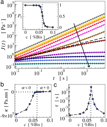
Figure 3: (a) Compliance $J(t)$ for different concentrations $c$ of bis-acrylamide cross-linker. Symbols denote the data obtained from the master curves (see Fig. 2) by using the experimentally obtained shift factors $\text{a}_{c}$ and $\text{b}_{c}$ of Ref. Larsen and Furst (2008), while continuous lines correspond to the fit of the data points to Eq. 37. The dashed line denote a curve proportional to $t^{n}$ with $n=0.55$, which lies between the sol and gel phases, and the arrow indicate the increasing concentration of cross-linker $c$. Inset shows the effective exponent of $J(t)$, Eq. 40, for different concentrations at $t=1\,$s. (b) and (c) are, respectively, the elastic constant $\kappa$ and the relaxation time $\tau$ obtained from the fit of the data displayed in (a) to Eq. 37 with the same exponents $\alpha$ and $n$ used in Fig. 2. The vertical dotted lines indicate the critical concentration of cross-linkers $c^{*}$.

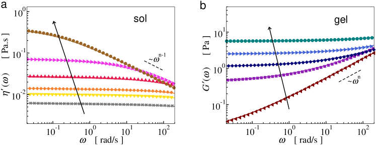
Figure 4: (a) and (b) show the viscosity $\eta^{\prime}(\omega)=G^{\prime\prime}(\omega)/\omega$ and the storage modulus $G^{\prime}(\omega)$ at different concentrations $c$ of cross-linkers, respectively. Arrows indicate the increasing concentration $c$ of cross-linkers. Symbols correspond to data obtained numerically from the curves $J(t)$ presented in Fig. 3 by using the method proposed in Ref. Evans et al. (2009), while continuous lines corresponds to Eqs. 42, $G^{\prime}(\omega)$, and 43, $\eta^{\prime}(\omega)$, with the exponents $\alpha$ and $n$ obtained from Fig. 2, and the values of $\kappa$ and $\tau$ extracted from the data presented in Figs. 3(b) and 3(c), respectively. For both $\eta^{\prime}(\omega)$ and $G^{\prime}(\omega)$ the relative difference between the estimates obtained by the two approaches is less than 0.1. Dashed lines indicate the behaviors at high frequencies: $\eta^{\prime}(\omega)\propto\omega^{n-1}$ and $G^{\prime}(\omega)\propto\omega^{n}$.

Unfortunately, it is difficult to evaluate an exact and general expression (i.e., for any values of $n$, $\alpha$, $\tau$ and $\kappa$) for the Fourier-Laplace transform of the Eq. 37. However, one can obtain approximated results by assuming that the compliance can be expanded around a time $t=1/\omega$ as Mason (2000)

$$J(t)\approx J(1/\omega)(\omega t)^{p(\omega)}$$ (38)

where $p(\omega)\equiv p(t)|_{t=1/\omega}$ is an effective exponent of the compliance (or, equivalently, of the MSD) around a time $t=1/\omega$, with $p(t)$ given by

$$p(t)=\frac{d\ln\langle\Delta r^{2}(t)\rangle}{d\ln t}=2d\frac{D(t)}{\langle\Delta r^{2}(t)\rangle}t~{}~{}.$$ (39)

By considering $\langle\Delta r^{2}(t)\rangle$ and $D(t)$ given by Eqs. 34 and 35, respectively, Eq. 39 yields

$$p(\upsilon)=\alpha n\frac{(\upsilon^{-1}-1)}{(1-\upsilon^{\alpha})}~{}~{},$$ (40)

with $\upsilon=\upsilon(t)=1+(t/\tau)^{n}$. One can check that, at short times ($t\ll\tau$), $\upsilon\approx 1$, thus $p=n$ for both $\alpha>0$ and $\alpha<0$, which is consistent to what is observed for the MSD in Figs. 2(a) and  2(b), and for $J(t)$ in Fig. 4(a). For long times ($t\gg\tau$), $\upsilon\approx(t/\tau)^{n}$ so that $p=-\alpha n\approx 1$ for $\alpha<0$ (sol phase), and $p(t)=\alpha n(t/\tau)^{-\alpha n}\approx 0$ for $\alpha>0$ (gel phase), in agreement to Figs. 2(a) and 2(b), and Fig. 4(a) as well. As illustrated in the inset of Fig. 3(a), one can use Eq. 40 to obtain the exponent $p_{1}$ at given time, e.g., $t=1\,$s, for the different values of $c$ in order to estimate the gelation concentration $c^{*}$ (see, e.g., Ref. Larsen et al. (2009)).

Hence, one can consider Eq. 38 to obtain an estimate of $\hat{J}(\omega)$ through a Fourier-Laplace integral, i.e., $\hat{J}(\omega)\approx J(1/\omega)\mathcal{L}[(\omega t)^{p(\omega)};s]_{s=i\omega}$, which leads to

$$i\omega\hat{J}(\omega)\approx J(1/\omega)\,\Gamma(1+p(\omega))\,e^{-i\pi p(\omega)/2}~{}~{}.$$ (41)

As previously mentioned, $\Gamma(1+p(\omega))$ denotes the usual gamma function Gradshteyn and Ryzhik (2007). The above expression is valid for $p(\omega)>-1$, so it can be used to describe all types of diffusive regimes, including the subdiffusion observed in restricted random walks where $p\approx 0$. Finally, by considering Eq. 41, one can use Eq. 3 to evaluate the storage modulus $G^{\prime}(\omega)$ and the viscosity $\eta^{\prime}(\omega)=G^{\prime\prime}(\omega)/\omega$, which are given, respectively, as

$$G^{\prime}(\omega)\approx g(\omega)\left(\frac{\kappa}{3\pi a}\right)\cos\left[\frac{\pi p(\omega)}{2}\right]~{}~{},$$ (42)

and

$$\eta^{\prime}(\omega)\approx\frac{g(\omega)}{\omega}\left(\frac{\kappa}{3\pi a}\right)\sin\left[\frac{\pi p(\omega)}{2}\right]~{}~{},$$ (43)

where

$$g(\omega)=\frac{1}{\{1-[(\omega\tau)^{-n}+1]^{-\alpha}\}\Gamma(1+p(\omega))}$$ (44)

with $p(\omega)$ obtained from Eq. 40 assuming that $\upsilon(\omega)=\upsilon(t)|_{t=1/\omega}=1+(\omega\tau)^{-n}$.

Figures 4(a) and 4(b) include a comparison between the viscosity $\eta^{\prime}(\omega)$ (at the sol phase) and the storage modulus $G^{\prime}(\omega)$ (at the gel phase) evaluated from Eqs. 42 and 43, and computed directly from the compliance $J(t)$ presented in Fig. 3(a) via the numerical method proposed in Ref. Evans et al. (2009). At high frequencies, $\omega\gg\tau^{-1}$, one have that $p\approx n$ and $g(\omega)\approx\alpha^{-1}(\omega\tau)^{n}/\Gamma(1+n)$, so that, just as discussed in Sec. II.5.3, one have that $G^{\prime}(\omega)\propto\omega^{n}$ and $G^{\prime\prime}(\omega)\propto\omega^{n}$, which leads to $\eta^{\prime}(\omega)\propto\omega^{n-1}$, as shown in Fig. 4.

For the sol phase ($\alpha<0$) at low frequencies, $\omega_{0}\ll\tau^{-1}$, Eqs. 40 and 44 lead to $p(\omega_{0})=-\alpha n$ and $g(\omega_{0})\approx-(\omega_{0}\tau)^{-\alpha n}$, respectively. Thus, one can consider Eq. 43 to obtain a limit for the viscosity at low frequencies, that is

$$\eta^{\prime}(\omega_{0})=-\frac{\kappa}{3\pi a}\,\omega_{0}^{-(1+\alpha n)}\,\tau^{-\alpha n}~{}~{}.$$ (45)

By taking $\alpha n\approx-1$, the above equation yields a value $\eta_{0}=\eta^{\prime}(\omega_{0})$ which is practically independent of the frequency $\omega_{0}$, as shown in Fig. 4(a). Also, it yields

$$\kappa\approx-3\pi a\frac{\eta_{0}}{\tau}~{}~{},$$ (46)

which corresponds to the same relation obtained from the limit for long times of the time-dependent diffusion coefficient $D(t)$ in Sec. III.2. In addition, at the sol phase, the low frequency value of the storage modulus given by Eq. 42 can be estimated as

$$G^{\prime}(\omega_{0})\approx\,C_{s}\,\eta_{0}\,\omega_{0}~{}~{},$$ (47)

where $\eta_{0}$ is defined as in Eq. 46, and $C_{s}=\pi(1+\alpha n)/2$ with $\alpha n\approx-1$. As expected, for $\alpha<0$ (sol phase), $G^{\prime}(\omega_{0})$ is proportional to $\omega_{0}$, which is a characteristic behavior of complex solutions at low frequencies.

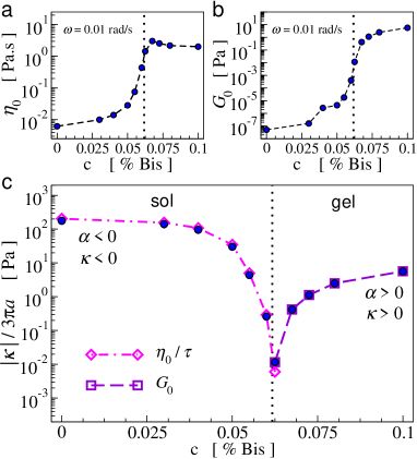
Figure 5: (a) and (b) show, respectively, the viscosity $\eta^{\prime}(\omega_{0})$ and the storage modulus $G^{\prime}(\omega_{0})$ obtained from the data presented in Figs. 4(a) and 4(b) at a low frequency, $\omega_{0}=0.01\,$rad/s, for different concentrations of cross-linkers $c$. (c) Validation of Eqs. 46 and 49: filled circles correspond to the modulus of the effective elastic constant, i.e. $|\kappa|/3\pi a$; the values of $\eta_{0}$ and $G_{0}$ are those displayed in (a) and (b), respectively, while the value of $\tau$ is obtained from Fig. 3(c). The vertical dotted lines indicate the critical concentration of cross-linkers $c^{*}$.

At the gel phase, one have that $\alpha>0$, then, at low frequencies ($\omega_{0}\ll\tau^{-1}$), Eqs. 40 and 44 lead to $p(\omega_{0})=\alpha n(\omega_{0}\tau)^{\alpha n}$ and $g(\omega_{0})\approx 1$, respectively. Hence, one can use Eq. 42 to obtain the limit of the storage modulus at low frequencies, that is

$$G^{\prime}(\omega_{0})\approx\frac{\kappa}{3\pi a}~{}~{},$$ (48)

which corresponds to the plateau value showed in Fig. 4(b). And, by assuming that $G_{0}\equiv G^{\prime}(\omega_{0})$ at the gel phase, one have that

$$\kappa\approx 3\pi a\,G_{0}~{}~{}.$$ (49)

Also, at low frequencies and $\alpha>0$, Eq. 43 yields

$$\eta^{\prime}(\omega_{0})=C_{g}\,G_{0}\,\tau^{\alpha n}\,\omega_{0}^{-(1-\alpha n)}~{}~{},$$ (50)

where $G_{0}$ is defined by Eq. 49 and $C_{g}=\alpha n(\pi/2)$.

Figures 5(a) and 5(b) show, respectively, $\eta^{\prime}(\omega_{0})$ and $G^{\prime}(\omega_{0})$ obtained from the data presented in Figs. 4(a) and 4(b) at a constant low frequency, $\omega_{0}=0.01\,$rad/s, as a function of the concentration of cross-linkers $c$ through the sol-gel transition for the polyacrylamide. At the sol phase, the low frequency values of the viscosity and the storage modulus are given by Eqs. 45 and 47, respectively. At the gel phase, the storage modulus can be described by Eq. 48, while the viscosity is given by Eq. 50.

Finally, I emphasize that Eqs. 46 and 49 establish relationships between the effective elastic constant $\kappa$ defined in the Langevin equation, Eq. 4, and the rheological properties of the viscoelastic material, i.e. $\eta_{0}/\tau$ at the sol phase, and $G_{0}$ at the gel phase. Figure 5(c) illustrates this correspondence through the sol-gel transition, by presenting the values of the modulus of the effective elastic constant, $|\kappa|/3\pi a$, together with the values of $\eta_{0}/\tau$ and $G_{0}$ obtained from the data in Figs. 4(a) and 4(b).

IV Concluding remarks

In this paper I consider an approach based on microrheology to provide a general expression for the mean-squared displacement of probe particles which can be used to obtain the full viscoelastic response of gels. The non-markovian Langevin approach used here allowed me to establish useful interrelations between the MSD of probe particles, Eq. 34, and several functions, in particular, the response function $\chi(t)$, Eq. 31, the time-dependent diffusion coefficient $D(t)$, Eq. 35, the memory kernels $b(t)$ and $u(t)$ of the Langevin equations, Eqs. 4 and 21, and also to the memory functions $\psi(t)$, Eq. 32, and $\beta(t)$, Eq. 33, which are related to the Fokker-Plank equation, Eq. 17.

The expressions obtained for the viscoelastic response of the gel, i.e., the storage modulus, Eq. 42, and the viscosity, Eq. 43, should be of practical interest to both theoreticians and experimentalists. For instance, those equations might be used to describe rheological/microrheological data providing estimates for the exponents $n$ and $\alpha$ which characterize, respectively, the dynamics and the structures of the gel. In particular, Eq. 43 can be seen as an alternative model (e.g., Cross, Carreau, Bird) to viscosity, specially for shear-thinning viscoelastic materials, which present a decreasing $\eta^{\prime}(\omega)$ similar as those displayed in Fig. 4(a). Also, the analytical expressions which link the effective elastic constant $\kappa$ introduced in the Langevin equations to the viscoelastic properties of the gel, i.e. Eqs. 46 and 47 (sol phase), and Eqs. 49 and 50 (gel phase), should provide a theoretical basis that goes beyond the analogy between gelation and percolation Adolf and Martin (1990); Martin and Adolf (1991), since those equations are expected to be valid not only at the sol-gel transition but in the coarsening regime as well Rizzi (2017); Rizzi, Auer, and Head (2016); Rizzi, Head, and Auer (2015).

It is worth mentioning that, due to experimental resolution of the available data, I consider that the exponent $\alpha$ changes abruptly from $-1/n$ to a finite positive value at the gelation point, even though the effective exponent $p_{1}$ changes continuosly (see the inset of Fig. 3(a)). However, for time-cure experiments involving physical gels, it could be that the changes in $\alpha$ are more notiaceable, and one might observe what is happening with it at the gelation point. In that case, just like in any microrheology experiment Rizzi and Tassieri , ergodicity breaking should be avoided by considering that the observation times $t_{\text{e}}$, i.e., the longest times used to probe the MSD, are much shorter than the cure times $t_{\text{w}}$. Hence, in order to use the framework developed here, one must assume that the distribution $\rho_{\alpha}(\varepsilon)$ defined by Eq. 30 remains unaltered for times $t<t_{\text{e}}\ll t_{\text{w}}$.

Finally, one should note that I derived the expression for the MSD from a distribution of elastic constants which might be related to the cluster sizes distribution in the sample Krall, Huang, and Weitz (1997); Dinsmore et al. (2006). Thus, my results suggest that, besides of being interpreted as a generalization of the results obtained in Ref. Krall, Huang, and Weitz (1997), the expression obtained here for the MSD, Eq. 34, should be related to approaches that compute the relaxation modulus $G(t)$ from the time relaxation distribution $H(\lambda)$ through Eq. 1 as in, for instance, Ref. Winter and Chambon (1986). In fact, by assuming that $\xi=(\lambda/\tau)^{\gamma}$ and recalling that $\xi=\alpha\varepsilon/2\kappa$, one can consider the distribution of local elastic constants $\varepsilon$ defined by Eq. 30 to obtain the distribution of relaxation times $\lambda$ as

$$H(\lambda)=\frac{1}{\,\Gamma(\alpha/2)}\left|\frac{\gamma}{\tau}\right|\left(\frac{\lambda}{\tau}\right)^{\alpha\gamma/2-1}\exp\left[-\left(\frac{\lambda}{\tau}\right)^{\gamma}\,\right]~{}~{},$$ (51)

which is known as a generalized gamma distribution Crooks (2019). Remarkably, the above expression is similar to the semi-empirical distribution used in Ref. Zaccone et al. (2014) to obtain the complex modulus $G^{*}(\omega)$ of liquid-like solutions of colloidal particles from their self-assembly aggregation kinetics, and it is worth mentioning that one might explore it also to describe gel-like responses by considering negatives values for $\gamma$.

References

- Campbell and Garnett (1882) L. Campbell and W. Garnett, The Life of James Clerk Maxwell (MacMillan and Co., 1882).
- Maxwell (1877) J. C. Maxwell, “Constituion of bodies,” Ency. Brit. 1985-89, 310 (1877).
- Ferry (1980) J. D. Ferry, Viscoelastic Properties of Polymers, 3rd ed. (John Wiley & Sons, 1980).
- Larson (1999) R. G. Larson, The Structure and Rheology of Complex Fluids (Oxford University Press, 1999).
- Mours and Winter (2000) M. Mours and H. H. Winter, “Mechanical spectroscopy of polymers,” in Experimental methods in polymer science (Academic Press, 2000) Chap. 5, p. 495.
- Doi (2015) M. Doi, Soft Matter Physics (Oxford University Press, 2015).
- Rao (2014) M. A. Rao, Rheology of Fluid, Semisolid, and Solid Foods: Principles and Applications, 3rd ed. (Springer, 2014).
- Zaccarelli (2007) E. Zaccarelli, “Colloidal gels: Equilibrium and non-equilibrium routes,” J. Phys.: Condens. Matter 19, 323101 (2007).
- Flory (1953) P. J. Flory, Principles of Polymer Chemistry (Cornell University Press, 1953).
- de Gennes (1979) P.-G. de Gennes, Scaling Concepts in Polymer Physics (Cornell University Press, 1979).
- Rubinstein and Colby (2003) M. Rubinstein and R. H. Colby, Polymer Physics (Oxford University Press, 2003).
- Flory (1941) P. J. Flory, “Molecular size distribution in three dimensional polymers. I. gelation,” J. Am. Chem. Soc. 63, 3083 (1941).
- Stockmayer (1943) V. H. Stockmayer, “Theory of molecular size distribution and gel formation in branched-chain polymers,” J. Chem. Phys. 11, 45 (1943).
- Martin and Adolf (1991) J. E. Martin and D. Adolf, “The sol-gel transition in chemical gels,” Annu. Rev. Phys. Chem. 42, 311 (1991).
- Zaccone et al. (2014) A. Zaccone, H. H. W. H. H., M. Siebenbürger, and M. Ballauff, “Linking self-assembly, rheology, and gel transition in attractive colloids,” J. Rheol. 58, 1219 (2014).
- Krall, Huang, and Weitz (1997) A. H. Krall, Z. Huang, and D. A. Weitz, “Dynamics of density fluctuations in colloidal gels,” Physica A 235, 19 (1997).
- Krall and Weitz (1998) A. H. Krall and D. A. Weitz, “Internal dynamics and elasticity of fractal colloidal gels,” Phys. Rev. Lett. 80, 778 (1998).
- Mason and Weitz (1995) T. G. Mason and D. A. Weitz, “Optical measurements of frequency-dependent linear viscoelastic moduli of complex fluids,” Phys. Rev. Lett. 74, 1250 (1995).
- Waigh (2005) T. A. Waigh, “Microrheology of complex fluids,” Rep. Prog. Phys. 68, 685 (2005).
- Waigh (2016) T. A. Waigh, “Advances in the microrheology of complex fluids,” Rep. Prog. Phys. 79, 074601 (2016).
- (21) L. G. Rizzi and M. Tassieri, “Microrheology of biological specimens,” Encyclopedia of Analytical Chemistry (2018) .
- Squires and Mason (2010) T. M. Squires and T. G. Mason, “Fluid mechanics of microrheology,” Annu. Rev. Fluid Mech. 42, 413 (2010).
- Evans et al. (2009) R. M. L. Evans, M. Tassieri, D. Auhl, and T. A. Waigh, “Direct conversion of rheological compliance measurements into storage and loss moduli,” Phys. Rev. E 80, 012501 (2009).
- Larsen and Furst (2008) T. H. Larsen and E. M. Furst, “Microrheology of the liquid-solid transition during gelation,” Phys. Rev. Lett. 100, 146001 (2008).
- Larsen, Schultz, and Furst (2008) T. Larsen, K. Schultz, and E. M. Furst, “Hydrogel microrheology near the liquid-solid transition,” Korea-Australia Rheol. J. 20, 165 (2008).
- Corrigan and Donald (2009a) A. M. Corrigan and A. M. Donald, “Passive microrheology of solvent-induced fibrillar protein networks,” Langmuir 25, 8599 (2009a).
- Corrigan and Donald (2009b) A. M. Corrigan and A. M. Donald, “Particle tracking microrheology of gel-forming amyloid fibril networks,” Eur. Phys. J. E 28, 457 (2009b).
- Aufderhorst-Roberts et al. (2014) A. Aufderhorst-Roberts, W. J. Frith, M. Kirkland, and A. M. Donald, “Microrheology and microstructure of Fmoc-derivative hydrogels,” Langmuir 30, 4483 (2014).
- Rizzi (2017) L. G. Rizzi, “On the relationship between the plateau modulus and the threshold frequency in peptide gels,” J. Chem. Phys. 147, 244902 (2017).
- Adelman (1976) S. A. Adelman, “Fokker-Planck equations for simple non‐markovian systems,” J. Chem. Phys. 64 64, 124 (1976).
- Panja (2010a) D. Panja, “Generalized Langevin equation formulation for anomalous polymer dynamics,” J. Stat. Mech. 2010, L02001 (2010a).
- Panja (2010b) D. Panja, “Anomalous polymer dynamics is non-markovian: Memory effects and the generalized Langevin equation formulation,” J. Stat. Mech. 2010, P06011 (2010b).
- Sarmiento-Gomez, Santamaría-Holek, and Castillo (2014) E. Sarmiento-Gomez, I. Santamaría-Holek, and R. Castillo, “Mean-square displacement of particles in slightly interconnected polymer networks,” J. Phys. Chem. B 118, 1146 (2014).
- Azevedo and Rizzi (2020) T. N. Azevedo and L. G. Rizzi, “Microrheology of filament networks from Brownian dynamics simulations,” J. Phys.: Conf. Ser. 1483, 012001 (2020).
- Doi and Edwards (1986) M. Doi and S. F. Edwards, The Theory of Polymer Dynamics (Oxford University Press, 1986).
- (36) L. K. R. Duarte, A. V. N. C. Teixeira, and L. G. Rizzi, “Microrheology of semiflexible filament solutions based on relaxation simulations,” (arXiv:2005.13661) .
- Teixeira, Geissler, and Licinio (2007) A. V. Teixeira, E. Geissler, and P. Licinio, “Dynamic scaling of polymer gels comprising nanoparticles,” J. Phys. Chem. B 111, 340 (2007).
- Romer et al. (2014) S. Romer, H. Bissig, P. Schurtenberger, and F. Scheffold, “Rheology and internal dynamics of colloidal gels from the dilute to the concentrated regime,” Europhys. Lett. 108, 48006 (2014).
- Romer, Scheffold, and Schurtenberger (2000) S. Romer, F. Scheffold, and P. Schurtenberger, “Sol-gel transition of concentrated colloidal suspensions,” Phys. Rev. Lett. 85, 4980 (2000).
- Santamaría-Holek and Rubi (2006) I. Santamaría-Holek and J. M. Rubi, “Finite-size effects in microrheology,” J. Chem. Phys. 125, 064907 (2006).
- Calzolari et al. (2017) D. C. E. Calzolari, I. Bischofberger, F. Nazzani, and V. Trappe, “Interplay of coarsening, aging, and stress hardening impacting the creep behavior of a colloidal gel,” J. Rheol. 61, 817 (2017).
- Crooks (2019) G. E. Crooks, Field Guide to Continuous Probability Distributions (2019).
- Dinsmore et al. (2006) A. D. Dinsmore, V. Prasad, I. Y. Wong, and D. A. Weitz, “Microscopic structure and elasticity of weakly aggregated colloidal gels,” Phys. Rev. Lett. 96, 185502 (2006).
- Xue, Homans, and Radford (2009) W.-F. Xue, S. W. Homans, and S. E. Radford, “Amyloid fibril length distribution quantified by atomic force microscopy single-particle image analysis,” Protein Eng. Des. Sel. 22, 489 (2009).
- Gradshteyn and Ryzhik (2007) I. S. Gradshteyn and I. M. Ryzhik, Table of Integrals, Series, and Products (Academic Press, Elsevier, 2007).
- Satija and Makarov (2019) R. Satija and D. E. Makarov, “Generalized Langevin equation as a model for barrier crossing dynamics in biomolecular folding,” J. Phys. Chem. A 123, 802 (2019).
- Mason (2000) T. G. Mason, “Estimating the viscoelastic moduli of complex ̵̄uids using the generalized Stokes-Einstein equation,” Rheol. Acta 39, 371 (2000).
- Larsen et al. (2009) T. H. Larsen, M. C. Branco, K. Rajagopal, J. P. Schneider, and E. M. Furst, “Sequence-dependent gelation kinetics of -hairpin peptide hydrogels,” Macromolecules 42, 8443 (2009).
- Adolf and Martin (1990) D. Adolf and J. E. Martin, “Time-cure superposition during cross-linking,” Macromolecules 23, 3700 (1990).
- Rizzi, Auer, and Head (2016) L. G. Rizzi, S. Auer, and D. A. Head, “Importance of non-affine viscoelastic response in disordered fibre networks,” Soft Matter 12, 4332 (2016).
- Rizzi, Head, and Auer (2015) L. G. Rizzi, D. A. Head, and S. Auer, “Universality in the morphology and mechanics of coarsening amyloid fibril networks,” Phys. Rev. Lett. 114, 078102 (2015).
- Winter and Chambon (1986) H. H. Winter and F. Chambon, “Analysis of linear viscoelasticity of a crosslinking polymer at the gel point,” J. Rheol. 30, 367 (1986).