Residual-type a posteriori error analysis of HDG methods for Neumann boundary control problems

Abstract.

We study a posteriori error analysis of linear-quadratic boundary control problems under bilateral box constraints on the control which acts through a Neumann type boundary condition. We adopt the hybridizable discontinuous Galerkin method as discretization technique, and the flux variables, the scalar variables and the boundary trace variables are all approximated by polynomials of degree k. As for the control variable, it is discretized by the variational discretization concept. Then an efficient and reliable a posteriori error estimator is introduced, and we prove that the error estimator provides an upper bound and a lower bound for the error. Finally, numerical results are presented to illustrate the performance of the obtained a posteriori error estimator.

1. Introduction

Many optimization processes in science and engineering lead to optimal control problems where the sought state is a solution of a partial differential equation. The complexity of such problem needs special care in order to obtain efficient numerical approximations for the optimization problem. One particular method is adaptive finite element method, which can reduces the computational cost and boosts the accuracy of the numerical solutions by locally refining the meshes around the singularity.

Although the adaptive finite element method has become a popular approach for numerical solutions of partial differential equations since the work of Babuška and Rheinboldt [1], it has only quiet recently become popular for constrained optimal control problems. The pioneer work concerning a posteriori error analysis for distributed optimal control problems is published by Liu and Yan [25] for residual-type error estimators and Becker, Kapp, and Rannacher [2] for goal-oriented error estimators. Here, we further refer readers to [20, 27, 31, 32, 33] for residual-type estimators and [3, 21] for goal-oriented approach. Recently, in order to guarantee the performance of the a posteriori error estimator theoretically, many scholars have tried to prove the convergence of an adaptive finite element algorithm for distributed optimal control problems in [14, 15, 23, 28].

Compared to distributed optimal control problems, there exists limited work on a posteriori error analysis for boundary optimal control problems. In [26], the convex Neumann boundary control problem was considered on polygonal or Lipschitz piecewise $\mathcal{C}^{2}$ domain. Then a residual-type a posteriori error estimator was introduced, and the authors proved that the estimator provided an upper bound for the errors in the state and the control. In [19], by introducing a Lagrange multiplier, the authors derived an efficient and reliable residual-type a posteriori error estimator for Neumann boundary control problems on polygonal domain. In [22], Kohls, Rösch and Siebert derived a unifying framework for the a posteriori error analysis of control constrained linear-quadratic optimal control problems for the full and variational discretizations. In [4], Benner and Yücel investigated symmetric interior penalty Galerkin methods for Neumann boundary control problems with an extra coefficient in cost functional. By invoking a Lagrange multiplier associated with the control constraints, an efficient and reliable residual-type a posteriori error estimator was obtained for the errors in the state, adjoint, control and co-control. As for Dirichlet boundary control problems, we just mention [8, 16] and references therein for more details on a posteriori error analysis.

Recently, the hybridizable discontinuous Galerkin (HDG) methods [9], which keep the advantages of discontinuous Galerkin (DG) methods and result in a system with significantly reduced degrees of freedom, have been proposed for convection diffusion problem [13], interface problem [6], flow problem[29], optimal control problem [5, 17], and so on. In [10, 11, 12], Cockburn and Zhang studied HDG methods for second order elliptic problems, and an a posteriori error estimator with postprocessing solutions was obtained. To the best of our knowledge, there exists no work on residual-type a posteriori error analysis of HDG methods for boundary control problems.

In this paper, we investigate a posteriori error analysis of Neumann optimal control problems under bilateral box constraints on the control. The HDG method is used as discretization technique, and the flux variables, the scalar variables and the boundary trace variables are discretized by polynomials of degree $k$. As for the control variable, we adopt the variational discretization concept proposed by Hinze in [18] for approximation. Then an efficient and reliable residual-type a posteriori error estimator without any postprocessing solutions is introduced, and we prove that the error estimator provides not only an upper bound but also a lower bound up to data oscillations for the errors. Finally, numerical experiments are presented to validate the performance of the obtained estimator.

The remainder of the paper is arranged as follows: In Section 2 we introduce the model problem and the associated optimality system. In Section 3 the discrete optimality system is given, and we prove that the discrete scheme has a unique solution. Then we prove the reliability and efficiency of the error estimator in Section 4 and Section 5 respectively. Numerical experiments are presented in Section 6 to validate the performance of the obtained estimator. Finally, some conclusions are provided in Section 7.

Throughout this paper, let $C$ with or without subscript be a generic positive constant independent of the mesh size. For ease of exposition, we denote $A\leq CB$ by $A\lesssim B$.

2. The Neumann boundary control problem

Let $\Omega\in\mathbb{R}^{d}~{}(d=2,3)$ be a polygonal $(d=2)$ or polyhedral $(d=3)$ domain with boundary $\partial\Omega$. Before we introduce the model problem, let us summarize some notation. For bounded and open set $D\in\mathbb{R}^{d}$ or $D\in\mathbb{R}^{d-1}$, we denote the usual Sobolev spaces by $W^{s,p}(D)$ with norm $\|\cdot\|_{s,p,D}$ and seminorm $|\cdot|_{s,p,D}$. The Hilbertian Sobolev spaces are abbreviated by $H^{s}(D)=W^{s,2}(D)$ with norm $\|\cdot\|_{s,D}$ and seminorm $|\cdot|_{s,D}$. For $s=0$, $H^{0}(D)$ coincides with $L^{2}(D)$, and the inner product is denoted by $(\cdot,\cdot)_{D}$ for $D\in\mathbb{R}^{d}$ and $\langle\cdot,\cdot\rangle_{D}$ for $D\in\mathbb{R}^{d-1}$. Furthermore, we define $H(div,\Omega):=\{\textbf{v}\in(L^{2}(\Omega))^{d}:\nabla\cdot\textbf{v}\in L^{2}(\Omega)\}$.

Based on the domain $\Omega$, we consider the following Neumann boundary control problem

$$\min_{y\in H^{1}(\Omega),u\in U_{ad}}\mathcal{J}(y,u)=\frac{1}{2}\|y-y_{d}\|_{0,\Omega}^{2}+\frac{\alpha}{2}\|u\|_{0,\partial\Omega}^{2},$$ (1)

subject to the elliptic equations

$$-\Delta y+y =f\quad\rm{in}~{}\Omega,$$ (2a)

$$\nabla y\cdot\textbf{n} =u+g\quad\rm{on}~{}\partial\Omega,$$ (2b)

where the regularization parameter $\alpha$ is a positive constant, $y_{d}\in L^{2}(\Omega)$, $f\in L^{2}(\Omega)$, $g\in L^{2}(\partial\Omega)$, n is the unit vector normal to the boundary $\partial\Omega$. The set $U_{ad}$ of constraints is given by

$$U_{ad}=\{v\in L^{2}(\partial\Omega):u_{a}\leq v\leq u_{b}~{}a.e.~{}x\in\partial\Omega\},$$

where $u_{a}$ and $u_{b}$ are assumed to be constant, and that $u_{a}<u_{b}$.

From [24], we know that the Neumann boundary control problem (1)-(2) admits a unique solution $(y,u)\in H^{1}(\Omega)\times L^{2}(\partial\Omega)$, and there exists an adjoint-state $z\in H^{1}(\Omega)$ such that

$$-\Delta y+y =f\quad\rm{in}~{}\Omega,$$ (3a)

$$\nabla y\cdot\textbf{n} =u+g\quad\rm{on}~{}\partial\Omega,$$ (3b)

$$-\Delta z+z =y-y_{d}\quad\rm{in}~{}\Omega,$$ (3c)

$$\nabla z\cdot\textbf{n} =0\quad\rm{on}~{}\partial\Omega,$$ (3d)

$$\langle\alpha u+z,v-u\rangle_{\partial\Omega} \geq 0\quad\forall v\in U_{ad}.$$ (3e)

Moreover, the variational inequality (3e) is equivalent to the projection formula

$$u=\Pi_{U_{ad}}\Big{(}-\frac{1}{\alpha}z|_{\partial\Omega}\Big{)},$$ (4)

where $\Pi_{U_{ad}}$ is the $L^{2}$-projection onto $U_{ad}$. Then let $\textbf{p}=-\nabla y$ and $\textbf{q}=-\nabla z$, the optimality system (3) can be rewritten in a mixed form as follows:

$$\textbf{p}+\nabla y =0\quad\rm{in}~{}\Omega,$$ (5a)

$$\nabla\cdot\textbf{p}+y =f\quad\rm{in}~{}\Omega,$$ (5b)

$$-\textbf{p}\cdot\textbf{n} =u+g\quad\rm{on}~{}\partial\Omega,$$ (5c)

$$\textbf{q}+\nabla z =0\quad\rm{in}~{}\Omega,$$ (5d)

$$\nabla\cdot\textbf{q}+z =y-y_{d}\quad\rm{in}~{}\Omega,$$ (5e)

$$-\textbf{q}\cdot\textbf{n} =0\quad\rm{on}~{}\partial\Omega,$$ (5f)

$$\langle\alpha u+z,v-u\rangle_{\partial\Omega} \geq 0\quad\forall v\in U_{ad}.$$ (5g)

3. The HDG discretization

Let $\mathcal{T}_{h}$ be a conforming and shape regular partition of the domain $\Omega$. For each $K\in\mathcal{T}_{h}$, we denote $\partial K$ the set of its faces. Then we define $\partial\mathcal{T}_{h}=\{\partial K:K\in\mathcal{T}_{h}\}$. Denote $\mathcal{E}_{h}^{o}$ the set of all interior faces of $\mathcal{T}_{h}$ and $\mathcal{E}_{h}^{\partial}$ the set of all boundary faces of $\mathcal{T}_{h}$. Then we define $\mathcal{E}_{h}=\mathcal{E}_{h}^{o}\cup\mathcal{E}_{h}^{\partial}$. For any $K\in\mathcal{T}_{h}$ and $F\in\mathcal{E}_{h}$, $h_{K}$ and $h_{E}$ denote the diameters of the element $K$ and the face $F$ respectively. Furthermore, we define the mesh-dependent inner product by

$$(w,v)_{\mathcal{T}_{h}}=\sum_{K\in\mathcal{T}_{h}}(w,v)_{K},\quad\langle w,v\rangle_{\partial\mathcal{T}_{h}}=\sum_{K\in\mathcal{T}_{h}}\langle w,v\rangle_{\partial K}.$$

For vector-valued functions, the notations are similarly defined by the dot product.

Based on the partition $\mathcal{T}_{h}$, we define the discontinuous finite element spaces for the flux variables, the scalar variables and the boundary trace variables as following

$$\textbf{V}_{h}^{k}=\{\textbf{v}\in(L^{2}(\Omega))^{d}:\textbf{v}|_{K}\in(\mathcal{P}^{k}(K))^{d},~{}\forall K\in\mathcal{T}_{h}\},$$

$$W_{h}^{k}=\{w\in L^{2}(\Omega):w|_{K}\in\mathcal{P}^{k}(K),~{}\forall K\in\mathcal{T}_{h}\},$$

$$M_{h}^{k}=\{\mu\in L^{2}(\mathcal{E}_{h}):\mu|_{F}\in\mathcal{P}^{k}(F),~{}\forall F\in\mathcal{E}_{h}\},$$

where $\mathcal{P}^{k}(S)$ is the set of polynomials of degree no larger than $k$ on the domain $S$. In this paper, we adopt the variational concept proposed by Hinze [18] for the control variable, which suggests to approximate the state equation but not the control variable. Therefore the control variable will be implicitly discretized by formula (4). Then the HDG scheme of the system (5) reads as follows: Find $(\textbf{p}_{h},y_{h},\widehat{y}_{h})\in\textbf{V}_{h}^{k}\times W_{h}^{k}\times M_{h}^{k}$, $(\textbf{q}_{h},z_{h},\widehat{z}_{h})\in\textbf{V}_{h}^{k}\times W_{h}^{k}\times M_{h}^{k}$ and $u_{h}\in U_{ad}$ such that

$$(\textbf{p}_{h},\textbf{r}_{1})_{\mathcal{T}_{h}}-(y_{h},\nabla\cdot\textbf{r}_{1})_{\mathcal{T}_{h}}+\langle\widehat{y}_{h},\textbf{r}_{1}\cdot\textbf{n}\rangle_{\partial\mathcal{T}_{h}} =0,$$ (6a)

$$-(\textbf{p}_{h},\nabla w_{1})_{\mathcal{T}_{h}}+(y_{h},w_{1})_{\mathcal{T}_{h}}+\langle\widehat{\textbf{p}}_{h}\cdot\textbf{n},w_{1}\rangle_{\partial\mathcal{T}_{h}} =(f,w_{1})_{\mathcal{T}_{h}},$$ (6b)

$$\langle\widehat{\textbf{p}}_{h}\cdot\textbf{n},\mu_{1}\rangle_{\partial\mathcal{T}_{h}\backslash\partial\Omega} =0,$$ (6c)

$$-\langle\widehat{\textbf{p}}_{h}\cdot\textbf{n},\mu_{1}\rangle_{\partial\Omega} =\langle u_{h}+g,\mu_{1}\rangle_{\partial\Omega},$$ (6d)

$$(\textbf{q}_{h},\textbf{r}_{2})_{\mathcal{T}_{h}}-(z_{h},\nabla\cdot\textbf{r}_{2})_{\mathcal{T}_{h}}+\langle\widehat{z}_{h},\textbf{r}_{2}\cdot\textbf{n}\rangle_{\partial\mathcal{T}_{h}} =0,$$ (6e)

$$-(\textbf{q}_{h},\nabla w_{2})_{\mathcal{T}_{h}}+(z_{h},w_{2})_{\mathcal{T}_{h}}+\langle\widehat{\textbf{q}}_{h}\cdot\textbf{n},w_{2}\rangle_{\partial\mathcal{T}_{h}} =(y_{h}-y_{d},w_{2})_{\mathcal{T}_{h}},$$ (6f)

$$\langle\widehat{\textbf{q}}_{h}\cdot\textbf{n},\mu_{2}\rangle_{\partial\mathcal{T}_{h}\backslash\partial\Omega} =0,$$ (6g)

$$-\langle\widehat{\textbf{q}}_{h}\cdot\textbf{n},\mu_{2}\rangle_{\partial\Omega} =0,$$ (6h)

$$\langle\alpha u_{h}+\widehat{z}_{h},v-u_{h}\rangle_{\partial\Omega} \geq 0,$$ (6i)

for any $(\textbf{r}_{1},w_{1},\mu_{1})\in\textbf{V}_{h}^{k}\times W_{h}^{k}\times M_{h}^{k}$, $(\textbf{r}_{2},w_{2},\mu_{2})\in\textbf{V}_{h}^{k}\times W_{h}^{k}\times M_{h}^{k}$ and $v\in U_{ad}$. Similarly, we know that the inequality (6i) is equivalent to the following projection formula

$$u_{h}=\Pi_{U_{ad}}\Big{(}-\frac{1}{\alpha}\widehat{z}_{h}|_{\partial\Omega}\Big{)}.$$

Here the normal component of numerical fluxes $\widehat{\textbf{p}}_{h}\cdot\textbf{n}$ and $\widehat{\textbf{q}}_{h}\cdot\textbf{n}$ is defined as

$$\widehat{\textbf{p}}_{h}\cdot\textbf{n}=\textbf{p}\cdot\textbf{n}+\tau_{1}(y_{h}-\widehat{y}_{h})\quad\rm{on}~{}\partial\mathcal{T}_{h},$$

$$\widehat{\textbf{q}}_{h}\cdot\textbf{n}=\textbf{q}\cdot\textbf{n}+\tau_{2}(z_{h}-\widehat{z}_{h})\quad\rm{on}~{}\partial\mathcal{T}_{h},$$

for stabilization parameters $\tau_{1}$ and $\tau_{2}$.

For ease of exposition, we define operators $\mathcal{B}$ by

$$\mathcal{B}(\textbf{r}_{1},w_{1},\mu_{1};\textbf{r}_{2},w_{2},\mu_{2};\tau)$$

$$= (\textbf{r}_{1},\textbf{r}_{2})_{\mathcal{T}_{h}}-(w_{1},\nabla\cdot\textbf{r}_{2})_{\mathcal{T}_{h}}+\langle\mu_{1},\textbf{r}_{2}\cdot\textbf{n}\rangle_{\partial\mathcal{T}_{h}}$$

$$+(\nabla\cdot\textbf{r}_{1},w_{2})_{\mathcal{T}_{h}}+(w_{1},w_{2})_{\mathcal{T}_{h}}$$

$$+\langle\tau(w_{1}-\mu_{1}),w_{2}\rangle_{\partial\mathcal{T}_{h}}-\langle\textbf{r}_{1}\cdot\textbf{n}+\tau(w_{1}-\mu_{1}),\mu_{2}\rangle_{\partial\mathcal{T}_{h}},$$

Then the HDG scheme (6) can be rewritten according to the operator $\mathcal{B}$: Find $(\textbf{p}_{h},y_{h},\widehat{y}_{h})\in\textbf{V}_{h}^{k}\times W_{h}^{k}\times M_{h}^{k}$, $(\textbf{q}_{h},z_{h},\widehat{z}_{h})\in\textbf{V}_{h}^{k}\times W_{h}^{k}\times M_{h}^{k}$ and $u_{h}\in U_{ad}$ such that

$$\mathcal{B}(\textbf{p}_{h},y_{h},\widehat{y}_{h};\textbf{r}_{1},w_{1},\mu_{1};\tau_{1}) =(f,w_{1})_{\mathcal{T}_{h}}+\langle u_{h}+g,\mu_{1}\rangle_{\partial\Omega},$$ (7a)

$$\mathcal{B}(\textbf{q}_{h},z_{h},\widehat{z}_{h};\textbf{r}_{2},w_{2},\mu_{2};\tau_{2}) =(y_{h}-y_{d},w_{2})_{\mathcal{T}_{h}},$$ (7b)

$$\langle\alpha u_{h}+\widehat{z}_{h},v-u_{h}\rangle_{\partial\Omega} \geq 0,$$ (7c)

for any $(\textbf{r}_{1},w_{1},\mu_{1})\in\textbf{V}_{h}^{k}\times W_{h}^{k}\times M_{h}^{k}$, $(\textbf{r}_{2},w_{2},\mu_{2})\in\textbf{V}_{h}^{k}\times W_{h}^{k}\times M_{h}^{k}$ and $v\in U_{ad}$.

Theorem 3.1.

We assume that $\tau_{1}=\tau_{2}>0$ on $\partial\mathcal{T}_{h}$ and $0\in U_{ad}$. Then the system (7) has a unique solution.

Proof.

Since the system (7) is finite dimensional, we only need to prove that the system (7) just has the zero solution for the case of $f=y_{d}=g=0$. Let $(\textbf{r}_{1},w_{1},\mu_{1})=(\textbf{q}_{h},-z_{h},-\widehat{z}_{h})$ in (7a) and $(\textbf{r}_{2},w_{2},\mu_{2})=(-\textbf{p}_{h},y_{h},\widehat{y}_{h})$ in (7b), we have

$$0= \mathcal{B}(\textbf{p}_{h},y_{h},\widehat{y}_{h};\textbf{q}_{h},-z_{h},-\widehat{z}_{h};\tau_{1})+\mathcal{B}(\textbf{q}_{h},z_{h},\widehat{z}_{h};-\textbf{p}_{h},y_{h},\widehat{y}_{h};\tau_{2})$$

$$= (y_{h},y_{h})_{\mathcal{T}_{h}}-\langle u_{h},\widehat{z}_{h}\rangle_{\partial\Omega}\geq(y_{h},y_{h})_{\mathcal{T}_{h}}+\alpha\langle u_{h},u_{h}\rangle_{\partial\Omega},$$

from (7c) and the assumption $0\in U_{ad}$. Hence $y_{h}=0$ and $u_{h}=0$. Furthermore, let $(\textbf{r}_{1},w_{1},\mu_{1})=(\textbf{p}_{h},y_{h},\widehat{y}_{h})$ in (7a) and $(\textbf{r}_{2},w_{2},\mu_{2})=(\textbf{q}_{h},z_{h},\widehat{z}_{h})$ in (7b), we have

$$0= (\textbf{p}_{h},\textbf{p}_{h})_{\mathcal{T}_{h}}+(y_{h},y_{h})_{\mathcal{T}_{h}}+\langle\tau_{1}(y_{h}-\widehat{y}_{h}),y_{h}-\widehat{y}_{h}\rangle_{\partial\mathcal{T}_{h}},$$

$$0= (\textbf{q}_{h},\textbf{q}_{h})_{\mathcal{T}_{h}}+(z_{h},z_{h})_{\mathcal{T}_{h}}+\langle\tau_{2}(z_{h}-\widehat{z}_{h}),z_{h}-\widehat{z}_{h}\rangle_{\partial\mathcal{T}_{h}}$$

Therefore $\textbf{p}_{h}=0$, $\widehat{y}_{h}=0$, $\textbf{q}_{h}=0$, $z_{h}=0$ and $\widehat{z}_{h}=0$. Then we conclude the proof. ∎

4. The residual-type a posteriori error estimator

4.1. Auxiliary results

Before we start to prove a posteriori error estimator for the model problem, we first provide some auxiliary results that will play an important role in the proof.

For each element $K\in\mathcal{T}_{h}$ and face $F\in\mathcal{E}_{h}$, we denote $\Pi_{j}^{o}$ and $\Pi_{j}^{\partial}$ the $L^{2}$-projections onto $\mathcal{P}^{j}(K)$ and $\mathcal{P}^{j}(F)$ for the nonnegative integer $j$. Then, from [6] we have the following error estimates

Lemma 4.1.

For any $K\in\mathcal{T}_{h}$ and $F\in\mathcal{E}_{h}$, we have

$$\|\Pi_{j}^{o}v\|_{0,K}\leq \|v\|_{0,K}\quad\forall v\in L^{2}(K),$$

$$\|\Pi_{j}^{\partial}v\|_{0,F}\leq \|v\|_{0,F}\quad\forall v\in L^{2}(F),$$

$$\|v-\Pi_{0}^{o}v\|_{0,K}\lesssim h_{K}\|\nabla v\|_{0,K}\quad\forall v\in H^{1}(K),$$

$$\|v-\Pi_{0}^{o}v\|_{0,\partial K}\lesssim h_{K}^{1/2}\|\nabla v\|_{0,K}\quad\forall v\in H^{1}(K).$$

We conclude this subsection by introducing a lemma that has been proved in [7].

Lemma 4.2.

Let $F$ be a face of the element $K\in\mathcal{T}_{h}$, $\textbf{n}_{F}$ the unit vector normal to $F$, and $s>0$. Assume that $v$ is a given function in $H^{1+s}(K)$ and $\Delta v\in L^{2}(K)$. For any $w_{h}\in\mathcal{P}^{k}(F)$, we have

$$\langle\nabla v\cdot\textbf{n}_{F},w_{h}\rangle_{F}\lesssim h_{F}^{-1/2}\|w_{h}\|_{0,F}(\|\nabla v\|_{0,K}+h_{K}\|\Delta v\|_{0,K}).$$

4.2. Reliability of the error estimator

We begin this section by defining error estimators for each $K\in\mathcal{T}_{h}$ in the following

$$\eta_{s,K,1}= \|\textbf{p}_{h}+\nabla y_{h}\|_{0,K},\quad\quad\eta_{as,K,1}=\|\textbf{q}_{h}+\nabla z_{h}\|_{0,K},$$

$$\eta_{s,K,2}= h_{K}\|f-\nabla\cdot\textbf{p}_{h}-y_{h}\|_{0,K},\quad\eta_{as,K,2}=h_{K}\|y_{h}-y_{d}-\nabla\cdot\textbf{q}_{h}-z_{h}\|_{0,K},$$

$$\eta_{s,\partial K}= h_{K}^{-1/2}\|y_{h}-\widehat{y}_{h}\|_{0,\partial K},\quad\quad\eta_{as,\partial K}=h_{K}^{-1/2}\|z_{h}-\widehat{z}_{h}\|_{0,\partial K}.$$

Furthermore, we define

$$\eta_{s}^{2}=\sum_{K\in\mathcal{T}_{h}}\{\eta_{s,K,1}^{2}+\eta_{s,K,2}^{2}+\eta_{s,\partial K}^{2}\},$$

$$\eta_{as}^{2}=\sum_{K\in\mathcal{T}_{h}}\{\eta_{as,K,1}^{2}+\eta_{as,K,2}^{2}+\eta_{as,\partial K}^{2}\}.$$

Next, we consider the following auxiliary problem: Find $\textbf{p}(u_{h}),\textbf{q}(u_{h})\in H(div,\Omega)$ and $y(u_{h}),z(u_{h})\in H^{1}(\Omega)$ such that

$$\textbf{p}(u_{h})+\nabla y(u_{h}) =0\quad\rm{in}~{}\Omega,$$ (8a)

$$\nabla\cdot\textbf{p}(u_{h})+y(u_{h}) =f\quad\rm{in}~{}\Omega,$$ (8b)

$$-\textbf{p}(u_{h})\cdot\textbf{n} =u_{h}+g\quad\rm{on}~{}\partial\Omega,$$ (8c)

$$\textbf{q}(u_{h})+\nabla z(u_{h}) =0\quad\rm{in}~{}\Omega,$$ (8d)

$$\nabla\cdot\textbf{q}(u_{h})+z(u_{h}) =y(u_{h})-y_{d}\quad\rm{in}~{}\Omega,$$ (8e)

$$-\textbf{q}(u_{h})\cdot\textbf{n} =0\quad\rm{on}~{}\Omega.$$ (8f)

Now the error $\|u-u_{h}\|_{0,\partial\Omega}+\|\textbf{p}-\textbf{p}(u_{h})\|_{0,\Omega}+\|y-y(u_{h})\|_{0,\Omega}+\|\textbf{q}-\textbf{q}(u_{h})\|_{0,\Omega}+\|z-z(u_{h})\|_{0,\Omega}$ can be bounded by $\|z_{h}-z(u_{h})\|_{1,\Omega}$ and $\Big{\{}\sum_{K\in\mathcal{T}_{h}}\eta_{as,\partial K}^{2}\Big{\}}^{1/2}$.

Lemma 4.3.

Let $(u,\textbf{p},y,\textbf{q},z)$ and $(u_{h},\textbf{p}_{h},y_{h},\widehat{y}_{h},\textbf{q}_{h},z_{h},\widehat{z}_{h})$ be the solutions of problems (5) and (7) respectively. Moreover let $(\textbf{p}(u_{h}),y(u_{h}),\textbf{q}(u_{h}),z(u_{h}))$ as defined above. Then the following error estimate holds

$$\|u-u_{h}\|_{0,\partial\Omega}+\|\textbf{p}-\textbf{p}(u_{h})\|_{0,\Omega}+\|y-y(u_{h})\|_{0,\Omega}+\|\textbf{q}-\textbf{q}(u_{h})\|_{0,\Omega}$$

$$+\|z-z(u_{h})\|_{0,\Omega}\lesssim\Big{\{}\sum_{K\in\mathcal{T}_{h}}\eta_{as,\partial K}^{2}\Big{\}}^{1/2}+\|z_{h}-z(u_{h})\|_{1,\Omega}$$

Proof.

From (5), (8) and integration by parts to yield

$$\langle z-z(u_{h}),u-u_{h}\rangle_{\partial\Omega}=\|y-y(u_{h})\|_{0,\Omega}^{2}.$$ (9)

Obviously, $(\textbf{p}-\textbf{p}(u_{h}),y-y(u_{h}))$ is the solution of system (5a)- (5c) with $g=-u_{h}$ and $f=0$, and $(\textbf{q}-\textbf{q}(u_{h}),z-z(u_{h}))$ is the solution of system (5d)-(5f) with $y_{d}=y(u_{h})$. Therefore we have

$$\|\textbf{p}-\textbf{p}(u_{h})\|_{0,\Omega}+\|y-y(u_{h})\|_{0,\Omega} \lesssim\|u-u_{h}\|_{0,\partial\Omega},$$ (10)

$$\|\textbf{q}-\textbf{q}(u_{h})\|_{0,\Omega}+\|z-z(u_{h})\|_{0,\Omega} \lesssim\|y-y(u_{h})\|_{0,\Omega},$$ (11)

by the trace theorem. From (5g), (7c) and (9), we obtain

$$\alpha\|u-u_{h}\|_{0,\partial\Omega}^{2}\leq \langle\widehat{z}_{h}-z(u_{h}),u-u_{h}\rangle_{\partial\Omega}$$

$$\leq \|z_{h}-z(u_{h})\|_{1,\Omega}\|u-u_{h}\|_{0,\partial\Omega}$$

$$+\langle z_{h}-\widehat{z}_{h},(\textbf{p}-\textbf{p}(u_{h}))\cdot\textbf{n}\rangle_{\partial\Omega}$$

$$\lesssim \|z_{h}-z(u_{h})\|_{1,\Omega}\|u-u_{h}\|_{0,\partial\Omega}$$ (12)

$$+\Big{\{}\sum_{K\in\mathcal{T}_{h}}\eta_{as,\partial K}^{2}\Big{\}}^{1/2}\Big{(}\|\textbf{p}-\textbf{p}(u_{h})\|_{0,\Omega}$$

$$+\|y-y(u_{h})\|_{0,\Omega}\Big{)},$$

by the trace theorem and Lemma 4.2. Then we can conclude the proof by combining (10)-(12). ∎

Lemma 4.4.

Let $(\textbf{p}(u_{h}),y(u_{h}),\textbf{q}(u_{h}),z(u_{h}))$ and $(u_{h},\textbf{p}_{h},y_{h},\widehat{y}_{h},\textbf{q}_{h},z_{h},\widehat{z}_{h})$ be the solutions of problems (8) and (7), then the following error estimates hold

$$\|\nabla(y_{h}-y(u_{h}))\|_{0,K}\leq\eta_{s,K,1}+\|\textbf{p}_{h}-\textbf{p}(u_{h})\|_{0,K},$$ (13)

$$\|\nabla(z_{h}-z(u_{h}))\|_{0,K}\leq\eta_{as,K,1}+\|\textbf{q}_{h}-\textbf{q}(u_{h})\|_{0,K},$$ (14)

for each $K\in\mathcal{T}_{h}$.

Proof.

Since $\textbf{p}(u_{h})=-\nabla y(u_{h})$ and $\textbf{q}(u_{h})=-\nabla z(u_{h})$ in each $K\in\mathcal{T}_{h}$, we can obtain the error estimates (13) and (14) directly by the triangle inequality. ∎

Now we are ready to prove a posteriori error estimators for $\|\textbf{p}_{h}-\textbf{p}(u_{h})\|_{0,\Omega}+\|y_{h}-y(u_{h})\|_{0,\Omega}$ and $\|\textbf{q}_{h}-\textbf{q}(u_{h})\|_{0,\Omega}+\|z_{h}-z(u_{h})\|_{0,\Omega}$.

Lemma 4.5.

Let $(\textbf{p}(u_{h}),y(u_{h}),\textbf{q}(u_{h}),z(u_{h}))$ and $(u_{h},\textbf{p}_{h},y_{h},\widehat{y}_{h},\textbf{q}_{h},z_{h},\widehat{z}_{h})$ be the solutions of problems (8) and (7), then we have

$$\|\textbf{p}_{h}-\textbf{p}(u_{h})\|_{0,\Omega}+\|y_{h}-y(u_{h})\|_{0,\Omega}+\|\tau_{1}^{1/2}(y_{h}-\widehat{y}_{h})\|_{0,\partial\mathcal{T}_{h}}\lesssim\eta_{s},$$ (15)

$$\|\textbf{q}_{h}-\textbf{q}(u_{h})\|_{0,\Omega}+\|z_{h}-z(u_{h})\|_{0,\Omega}+\|\tau_{2}^{1/2}(z_{h}-\widehat{z}_{h})\|_{0,\partial\mathcal{T}_{h}}\lesssim\eta_{s}+\eta_{as},$$ (16)

for $\tau_{1}=\tau_{2}=h_{K}^{-1}$ on each $\partial K$ for all $K\in\mathcal{T}_{h}$, where

$$\|\cdot\|_{0,\partial\mathcal{T}_{h}}^{2}=\sum_{K\in\mathcal{T}_{h}}\|\cdot\|_{0,\partial K}^{2}.$$

Proof.

According to the definition of the operator $\mathcal{B}$ to infer that

$$\mathcal{B}(\textbf{p}(u_{h})-\textbf{p}_{h},y(u_{h})-y_{h},y(u_{h})-\widehat{y}_{h};\textbf{r},w,\mu;\tau_{1})=0,$$

for any $(\textbf{r},w,\mu)\in\textbf{V}_{h}^{k}\times W_{h}^{k}\times M_{h}^{k}$. Then from the above equality and the definition of the operator $\mathcal{B}$, we have

$$\|\textbf{p}_{h}-\textbf{p}(u_{h})\|_{0,\Omega}^{2}+\|y_{h}-y(u_{h})\|_{0,\Omega}^{2}+\|\tau_{1}^{1/2}(y_{h}-\widehat{y}_{h})\|_{0,\partial\mathcal{T}_{h}}^{2}$$

$$= \mathcal{B}(\textbf{p}(u_{h})-\textbf{p}_{h},y(u_{h})-y_{h},y(u_{h})-\widehat{y}_{h};\textbf{p}(u_{h})-\textbf{p}_{h},y(u_{h})-y_{h},y(u_{h})-\widehat{y}_{h};\tau_{1})$$

$$= \mathcal{B}(\textbf{p}(u_{h})-\textbf{p}_{h},y(u_{h})-y_{h},y(u_{h})-\widehat{y}_{h};\delta_{\textbf{p}},\delta_{y},\delta_{\widehat{y}};\tau_{1}),$$

where $\delta_{\textbf{p}}=\textbf{p}(u_{h})-\textbf{p}_{h}-\textbf{r}$, $\delta_{y}=y(u_{h})-y_{h}-w$, and $\delta_{\widehat{y}}=y(u_{h})-\widehat{y}_{h}-\mu$ for any $(\textbf{r},w,\mu)\in\textbf{V}_{h}^{k}\times W_{h}^{k}\times M_{h}^{k}$. By integration by parts we yield

$$\mathcal{B}(\textbf{p}(u_{h})-\textbf{p}_{h},y(u_{h})-y_{h},y(u_{h})-\widehat{y}_{h};\delta_{\textbf{p}},\delta_{y},\delta_{\widehat{y}};\tau_{1})$$

$$= -(\textbf{p}_{h}+\nabla y_{h},\delta_{\textbf{p}})_{\mathcal{T}_{h}}+(f-\nabla\cdot\textbf{p}_{h}-y_{h},\delta_{y})_{\mathcal{T}_{h}}$$

$$+\langle y_{h}-\widehat{y}_{h},\delta_{\textbf{p}}\cdot\textbf{n}\rangle_{\partial\mathcal{T}_{h}}+\langle\tau_{1}(\widehat{y}_{h}-y_{h}),\delta_{y}\rangle_{\partial\mathcal{T}_{h}}$$

$$-\langle(\textbf{p}(u_{h})-\textbf{p}_{h})\cdot\textbf{n}+\tau_{1}(\widehat{y}_{h}-y_{h}),\delta_{\widehat{y}}\rangle_{\partial\mathcal{T}_{h}}.$$

From (6c), (6d) and (8c), we arrive at

$$-\langle(\textbf{p}(u_{h})-\textbf{p}_{h})\cdot\textbf{n}+\tau_{1}(\widehat{y}_{h}-y_{h}),\delta_{\widehat{y}}\rangle_{\partial\mathcal{T}_{h}}=0.$$

Now we set $\textbf{r}=\Pi_{0}^{o}(\textbf{p}(u_{h})-\textbf{p}_{h})$ in the definition of $\delta_{\textbf{p}}$ and $w=\Pi_{0}^{o}(y(u_{h})-y_{h})$ in the definition of $\delta_{y}$. Then from Lemma 4.1 we have

$$-(\textbf{p}_{h}+\nabla y_{h},\delta_{\textbf{p}})_{\mathcal{T}_{h}}+(f-\nabla\cdot\textbf{p}_{h}-y_{h},\delta_{y})_{\mathcal{T}_{h}}$$

$$\lesssim \Big{\{}\sum_{K\in\mathcal{T}_{h}}\eta_{s,K,1}^{2}\Big{\}}^{1/2}\|\textbf{p}(u_{h})-\textbf{p}_{h}\|_{0,\Omega}$$

$$+\Big{\{}\sum_{K\in\mathcal{T}_{h}}\eta_{s,K,2}^{2}\Big{\}}^{1/2}\|\nabla(y(u_{h})-y_{h})\|_{0,\Omega},$$

and

$$\langle\tau_{1}(\widehat{y}_{h}-y_{h}),\delta_{y}\rangle_{\partial\mathcal{T}_{h}}$$

$$\lesssim \Big{\{}\sum_{K\in\mathcal{T}_{h}}\eta_{s,\partial K}^{2}\Big{\}}^{1/2}\|\nabla(y(u_{h})-y_{h})\|_{0,\Omega}.$$

By using Lemma 4.2 to yield

$$\langle y_{h}-\widehat{y}_{h},\delta_{\textbf{p}}\cdot\textbf{n}\rangle_{\partial\mathcal{T}_{h}}$$

$$= \sum_{K\in\mathcal{T}_{h}}\sum_{F\in\partial K}\langle y_{h}-\widehat{y}_{h},\delta_{\textbf{p}}\cdot\textbf{n}\rangle_{F}$$

$$\lesssim \Big{\{}\sum_{K\in\mathcal{T}_{h}}\eta_{s,\partial K}^{2}\Big{\}}^{1/2}\|\textbf{p}(u_{h})-\textbf{p}_{h}\|_{0,\Omega}$$

$$+\Big{\{}\sum_{K\in\mathcal{T}_{h}}\eta_{s,\partial K}^{2}\Big{\}}^{1/2}\Big{(}\Big{\{}\sum_{K\in\mathcal{T}_{h}}\eta_{s,K,2}^{2}\Big{\}}^{1/2}+\|y_{h}-y(u_{h})\|_{0,\Omega}\Big{)}.$$

Now we can obtain the approximation result (15) by combining Lemma 4.4, Young’s inequality and the above equalities and inequalities. Moreover, the error estimate (16) can be proved similarly. ∎

Remark 4.1.

Compared to the error estimators introduced in [10, 11, 12], the Lemma 4.5 provides an a posteriori error estimator without any postprocessing solutions, hence it is easer to calculate.

Combining Lemma 4.3, Lemma 4.4 and Lemma 4.5 results in the following reliability estimate

Theorem 4.1.

Let $(u,\textbf{p},y,\textbf{q},z)$ and $(u_{h},\textbf{p}_{h},y_{h},\widehat{y}_{h},\textbf{q}_{h},z_{h},\widehat{z}_{h})$ be the solutions of problems (5) and (7). Then we have the following error estimate

$$\|u-u_{h}\|_{0,\partial\Omega}+\|\textbf{p}-\textbf{p}_{h}\|_{0,\Omega}+\|y-y_{h}\|_{1,\Omega}$$

$$+\|\textbf{q}-\textbf{q}_{h}\|_{0,\Omega}+\|z-z_{h}\|_{1,\Omega}\lesssim\eta_{s}+\eta_{as},$$

for $\tau_{1}=\tau_{2}=h_{K}^{-1}$ on each $\partial K$ for all $K\in\mathcal{T}_{h}$.

5. Efficiency of the error estimator

In this section, we will prove that, up to data oscillations, the estimator $\eta_{s}+\eta_{as}$ also provides a lower bound for the error. Especially, we will show that the local contributions of the estimator can be bounded from above by the local constituents of the error and the associated data oscillations.

First of all, we define the data oscillations by

$$osc^{2}(f,\mathcal{T}_{h}) =\sum_{K\in\mathcal{T}_{h}}osc^{2}(f,K),$$

$$osc^{2}(y_{d},\mathcal{T}_{h}) =\sum_{K\in\mathcal{T}_{h}}osc^{2}(y_{d},K),$$

where

$$osc(f,K) =h_{K}\|f-\Pi_{k}^{o}f\|_{0,K},$$

$$osc(y_{d},K) =h_{K}\|y_{d}-\Pi_{k}^{o}y_{d}\|_{0,K}.$$

Obviously, $osc(f,K)$ and $osc(y_{d},K)$ are of same order with $\eta_{s,K,2}$ and $\eta_{as,K,2}$ for non smooth $f$ and $y_{d}$ and of higher order for smooth $f$ and $y_{d}$.

Next we denote by $\lambda_{i}^{K}$, $1\leq i\leq 3$, the barycentric coordinates of $K\in\mathcal{T}_{h}$ and refer to $E_{K}=27\Pi_{i=1}^{3}\lambda_{i}^{K}$ as the associated element bubble function. From [19], we have

$$\|p_{K}\|_{0,K}^{2}\lesssim(p_{K},p_{K}E_{K})_{K}\quad K\in\mathcal{T}_{h},$$ (17a)

$$\|p_{K}E_{K}\|_{0,K}\lesssim\|p_{K}\|_{0,K}\quad K\in\mathcal{T}_{h},$$ (17b)

$$\|p_{K}E_{K}\|_{1,K}\lesssim h_{K}^{-1}\|p_{K}\|_{0,K}\quad K\in\mathcal{T}_{h},$$ (17c)

for $p_{K}\in\mathcal{P}^{k}(K)$. Then the following error estimates hold.

Theorem 5.1.

Let $(u,\textbf{p},y,\textbf{q},z)$, $(\textbf{p}(u_{h}),y(u_{h}),\textbf{q}(u_{h}),z(u_{h}))$ and $(u_{h},\textbf{p}_{h},y_{h},\widehat{y}_{h},\\ \textbf{q}_{h},z_{h},\widehat{z}_{h})$ be the solutions of problems (5), (8) and (7) respectively. Then we have

$$\eta_{s,K,1}\leq \|\textbf{p}-\textbf{p}_{h}\|_{0,K}+\|\nabla(y-y_{h})\|_{0,K}\quad K\in\mathcal{T}_{h},$$ (18)

$$\eta_{s,K,2}\lesssim osc(f,K)+\|\textbf{p}-\textbf{p}_{h}\|_{0,K}+\|y-y_{h}\|_{0,K}\quad K\in\mathcal{T}_{h},$$ (19)

$$\sum_{K\in\mathcal{T}_{h}}\eta_{s,\partial K}^{2}\lesssim \|u-u_{h}\|_{0,\partial\Omega}^{2}+\|\textbf{p}-\textbf{p}_{h}\|_{0,\Omega}^{2}+\|y-y_{h}\|_{1,\Omega}^{2}+osc^{2}(f,\mathcal{T}_{h}),$$ (20)

and

$$\eta_{as,K,1}\leq \|\textbf{q}-\textbf{q}_{h}\|_{0,K}+\|\nabla(z-z_{h})\|_{0,K}\quad K\in\mathcal{T}_{h},$$ (21)

$$\eta_{as,K,2}\lesssim osc(y_{d},K)+\|\textbf{q}-\textbf{q}_{h}\|_{0,K}+\|z-z_{h}\|_{0,K}$$

$$+\|y-y_{h}\|_{0,K}\quad K\in\mathcal{T}_{h},$$ (22)

$$\sum_{K\in\mathcal{T}_{h}}\eta_{as,\partial K}^{2}\lesssim \|u-u_{h}\|_{0,\partial\Omega}^{2}+\|\textbf{q}-\textbf{q}_{h}\|_{0,\Omega}^{2}+\|z-z_{h}\|_{1,\Omega}^{2}$$

$$+\|y-y_{h}\|_{0,\Omega}^{2}+osc^{2}(y_{d},\mathcal{T}_{h}).$$ (23)

Proof.

Obviously, the inequalities (18) and (21) can be obtained directly by the triangle inequality. According to the definition of $\eta_{s,K,2}$ and the triangle inequality we know that

$$\eta_{s,K,2}\leq osc(f,K)+h_{K}\|\Pi_{k}^{o}f-\nabla\cdot\textbf{p}_{h}-y_{h}\|_{0,K}.$$

Setting $p_{K}=\Pi_{k}^{o}f-\nabla\cdot\textbf{p}_{h}-y_{h}$ we obtain

$$h_{K}^{2}\|p_{K}\|_{0,K}^{2}\lesssim h_{K}^{2}(\Pi_{k}^{o}f-f+f-\nabla\cdot\textbf{p}_{h}-y_{h},E_{K}p_{K})_{K}$$

$$= h_{K}^{2}(\Pi_{k}^{o}f-f,E_{K}p_{K})_{K}+h_{K}^{2}(\nabla\cdot(\textbf{p}-\textbf{p}_{h})+y-y_{h},E_{K}p_{K})_{K},$$

from (17a). Then we can obtain the error estimate (19) by using (17), Young’s inequality and the above two inequalities. And the approximation result (22) can be proved similarly. Now we turn to prove the error estimate (20). From the proof of Lemma 4.5, we have

$$\sum_{K\in\mathcal{T}_{h}}\eta_{s,\partial K}^{2}\lesssim \|\textbf{p}(u_{h})-\textbf{p}_{h}\|_{0,\Omega}^{2}+\|y(u_{h})-y_{h}\|_{1,\Omega}^{2}$$

$$+\sum_{K\in\mathcal{T}_{h}}\{\eta_{s,K,1}^{2}+\eta_{s,K,2}^{2}\}.$$

Then by using (10), (18), (19), the triangle inequality and the above inequality to infer that

$$\sum_{K\in\mathcal{T}_{h}}\eta_{s,\partial K}^{2}\lesssim\|u-u_{h}\|_{0,\partial\Omega}+\|\textbf{p}-\textbf{p}_{h}\|_{0,\Omega}^{2}+\|y-y_{h}\|_{1,\Omega}^{2}+osc^{2}(f,\mathcal{T}_{h}).$$

Therefore the approximation result (20) is derived. And the inequality (23) can be proved similarly. ∎

6. Numerical experiments

Now we provide two examples in order to examine the quality of the derived estimator. As we know, an adaptive algorithm consists of the loops ”SOLVE$\rightarrow$ESTIMATE$\rightarrow$MARK$\rightarrow$REFINE”. In this section, a fix-point iteration algorithm presented in [34] is used for solving the model problem. In step REFINE, the newest vertex bisection algorithm [30] is employed, and the following marking strategy is used in step MARK

$$\sum_{K\in\mathcal{M}_{h}}\eta_{K}^{2}\geq\theta\eta^{2},$$

where

$$\eta^{2}=\eta_{s}^{2} +\eta_{as}^{2},$$

$$\eta_{K}^{2}=\eta_{s,K,1}^{2}+\eta_{s,K,2}^{2}+\eta_{s,\partial K}^{2} +\eta_{as,K,1}^{2}+\eta_{as,K,2}^{2}+\eta_{as,\partial K}^{2}.$$

Furthermore, we define

$$E= \|u-u_{h}\|_{0,\partial\Omega}+\|\textbf{p}-\textbf{p}_{h}\|_{0,\Omega}+\|y-y_{h}\|_{1,\Omega}$$

$$+\|\textbf{q}-\textbf{q}_{h}\|_{0,\Omega}+\|z-z_{h}\|_{1,\Omega}.$$

Here, we note that the figures of convergence history are plotted in log-log coordinates.

Example 6.1.

Based on the domain $\Omega=(0,1)^{2}$, we consider an example with $u_{a}=-0.1$, $u_{b}=0.1$ and $\alpha=1$. Let the functions $f$, $y_{d}$ and $g$ be such that the Neumann boundary control problem has the following exact solutions

$$y=\sin(2\pi x_{1})\sin(2\pi x_{2}),\quad z=\cos(2\pi x_{1}),\quad u=\Pi_{U_{ad}}\Big{\{}-\frac{1}{\alpha}z|_{\partial\Omega}\Big{\}}.$$

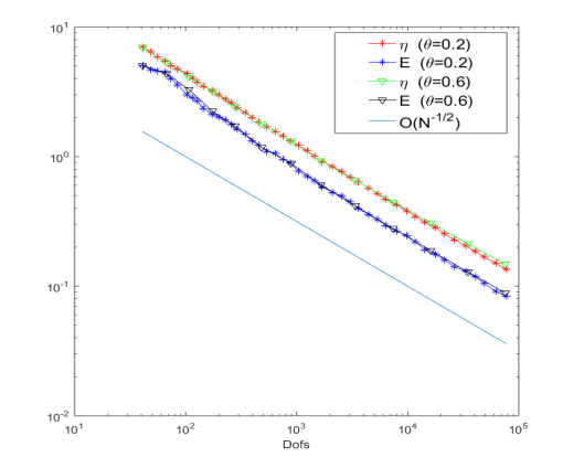
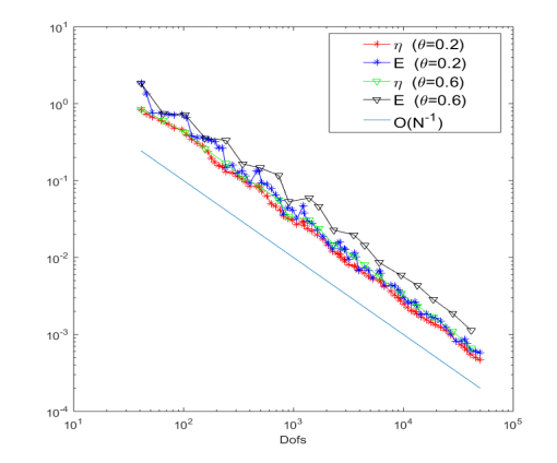
Figure 1. Left: Convergence history for $k=1$. Right: Convergence history for $k=2$.

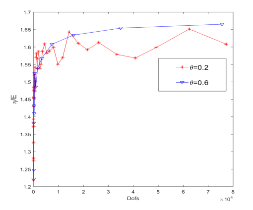
Figure 2. Left: The effectiveness index for $k=1$. Right: The effectiveness index for $k=2$.

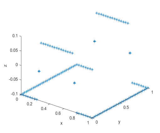
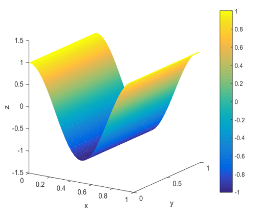
Figure 3. Left: The profile of the numerical control for $k=1$. Right: The profile of the numerical adjoint state for $k=1$.

We test the example for $k=1$ and $k=2$. From the convergence history in Figure 1 for $\theta=0.2$ and $\theta=0.6$, we find that the error $E$ is equivalent to the estimator $\eta$ and the error $E$ and the estimator $\eta$ can achieve the optimal convergence order by adaptive refinement. Furthermore, the effectiveness index is presented in Figure 2, which indicates the obtained a posteriori error estimator is very efficient. Finally, the profiles of the numerical control and adjoint state are shown in Figure 3.

Example 6.2.

We consider an example with a boundary term $\int_{\partial\Omega}yg_{1}dx$ in the objective functional. Then the adjoint problem possesses the Nuemann boundary condition $\nabla z\cdot\textbf{n}=g_{1}$. Here the designed domain is given by $\Omega=(-1,1)^{2}\backslash([0,1]\\ \times(-1,0])$. The control constraints and the regularization parameter are set as $u_{a}=-0.2$, $u_{b}=0.2$ and $\alpha=1$. Furthermore let the functions $f$, $y_{d}$ and $g$ be such that the Neumann boundary control problem has the following exact solutions

$$y(r,\theta_{1}) =0.$$

$$z(r,\theta_{1}) =r^{2/3}\cos\Big{(}\frac{2}{3}\theta_{1}\Big{)},$$

$$u(r,\theta_{1}) =\Pi_{U_{ad}}\Big{(}-r^{2/3}\cos\Big{(}\frac{2}{3}\theta_{1}\Big{)}\Big{)},$$

where $r=\sqrt{x_{1}^{2}+x_{2}^{2}}$, $\theta_{1}=\arccos(r^{-1}x\cdot e_{1})$ and $e_{1}=[1,0]^{T}$.

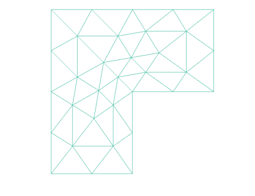
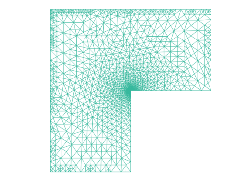
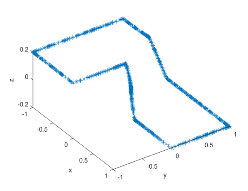
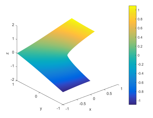
Figure 4. The profiles of the initial mesh (Top-Left), the adaptive mesh (Top-Right), the numerical control (Bottom-Left) and the numerical adjoint state (Bottom-Right) for $k=2$ and $\theta=0.4$.

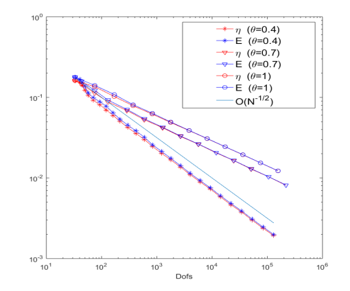
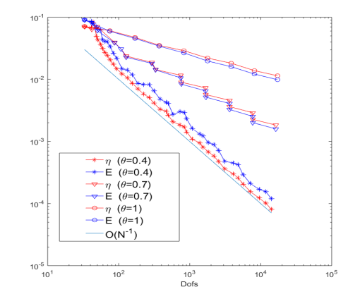
Figure 5. The convergence history for $k=1$ (Left) and $k=2$ (Right).

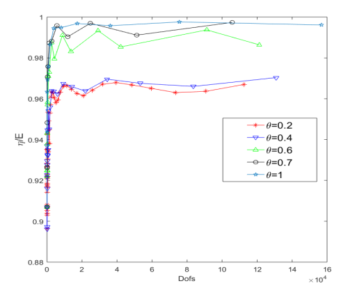
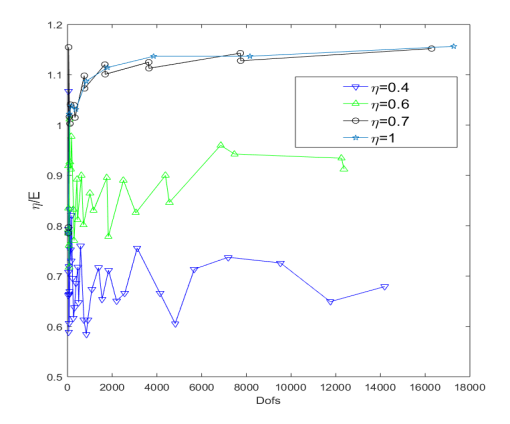
Figure 6. The effectiveness index for $k=1$ (Left) and $k=2$ (Right).

The adjoint exhibits a typical singularity at the reentrant corner of the domain $\Omega$. In Figure 4, we show the profiles of the initial mesh, the adaptive mesh, the numerical control and the numerical adjoint state for $k=2$ and $\theta=0.4$. We can find that the mesh nodes are concentrated around the reentrant corner where the singularity is induced. Hence the obtained a posteriori error estimator can grab efficiently the singularity of the problem. In Figure 5, the convergence history for $k=1$ and $k=2$ is presented, which indicates that the estimator $\eta$ is equivalent to the error $E$ and the estimator $\eta$ and the error $E$ can achieve the optimal convergence order while $\theta$ is less than a certain value. In Figure 6, the effectiveness index for $k=1$ and $k=2$ are provided. We can find that the effectiveness index for $k=1$ is between 0.96 and 1 and the effectiveness index for $k=2$ is between 0.6 and 1.2, which means the obtained a posteriori error estimator is very efficient.

7. Conclusions

In this paper, a Neumann boundary optimal control problem is considered. We use the hybridizable discontinuous Galerkin method as the discretization technique, and the flux variables, the scalar variables and the boundary trace variables are approximated by polynomials of degree $k$. Then an efficient and reliable a posteriori error estimator without any postprocessing solutions is obtained for the errors. Finally, two numerical experiments are provided to verify the performance of the obtained a posteriori error estimator.

This work is just the first step for a posteriori error analysis of HDG methods for boundary control problems. Next we extend the method and the result to the more complicated situations for instance the Dirichlet boundary control problem and the Stokes optimal control problem.

References

- [1] I. Babuška and W.C. Rheinboldt, Error estimates for adaptive finite element computations. SIAM J. Numer. Anal. 15 (1978) 736-754.
- [2] R. Becker, H. Kapp and R. Rannacher, Adaptive finite element methods for optimal control of partial differential equations: Basic concept. SIAM J. Control Optim. 39 (2000) 113-132.
- [3] O. Benedix and B. Vexler, A posteriori error estimation and adaptivety for elliptic optimal control problems with state constraints. Comput. Optim. Appl. 44 (2009) 3-25.
- [4] P. Benner and H. Yücel, Adaptive symmetric interior penalty Galerkin method for boundary control problems. SIAM J. Numer. Anal. 55 (2017) 1101-1133.
- [5] G. Chen, W. Hu, J. Shen, J. Singler, Y. Zhang and X. Zhang, An HDG method for distributed control of convection diffusion PDEs. J. Comput. Appl. Math. 343 (2018) 643-661.
- [6] G. Chen and J. Cui, On the error estimates of a hybridizable discontinuous Galerkin method for second-order elliptic problem with discontinuous coefficients. IMA J. Numer. Anal. 0 (2019) 1-24.
- [7] Z. Cai, C. He and S. Zhang, Discontinuous finite element methods for interface problem: Robus a priori and a posteriori error estimates. SIAM J. Numer. Anal. 55 (2017) 400-418.
- [8] S. Chowdhury, T. Gudi and A.K. Nandakumaran, Error bounds for a Dirichlet boundary control problem based on energy spaces. Math. Comp. 86 (2017) 1103-1126.
- [9] B. Cockburn, J. Gopalakrishnan and R. Lazarov, Unified hybridization of discontinuous Galerkin, mixed, and continuous Galerkin methods for second order elliptic problems. SIAM J. Numer. Anal. 47 (2009) 1319-1365.
- [10] B. Cockburn and W. Zhang, A posteriori error estimates for HDG methods. J. Sci. Comput. 51 (2012) 582-607.
- [11] B. Cockburn and W. Zhang, A posteriori error analysis for hybridizable discontinuous Galerkin methods for second order elliptic problems. SIAM J. Numer. Anal. 51 (2013) 676-693.
- [12] B. Cockburn and W. Zhang, An a posteriori error estimate for the variable-degree Raviart-Thomas method. Math. Comp. 83 (2013) 1063-1082.
- [13] G. Fu, W. Qiu and W. Zhang, An analysis of HDG methods for convection-dominated diffusion problems. ESIAM: M2AN 49 (2015) 225-256.
- [14] A. Gaevskaya, Y. Iliash, M. Kieweg and R.H.W. Hoppe, Convergence analysis of an adaptive finite element method for distributed control problems with control constraints. Control of Coupled Partial Differential Equations, Birkhäuser, Basel, (2007) 47-68.
- [15] W. Gong and N. Yan, Adaptive finite element method for elliptic optimal control problems: Convergence and optimality. Numer. Math. 135 (2017) 1121-1170.
- [16] W. Gong, W. Liu, T. Tan and N. Yan, A convergent adaptive finite element method for elliptic Dirichlet boundary control problems. IMA J. Numer. Anal. 0 (2018) 1-31.
- [17] W. Gong, W. Hu, M. Mateos, J. Singler, X. Zhang and Y. Zhang, A new HDG method for Dirichlet boundary control of convection diffusion PDEs II: Low regularity. SIAM J. Numer. Anal. 56 (2018) 2262-2287.
- [18] M. Hinze, A variational discretization concept in control constrained optimization: The linear quadratic case. Comput. Optim. Appl. 30 (2005) 45-61.
- [19] R.H.W. Hoppe, Y. Iliash, C. Iyyunni and N.H. Sweilam, A posteriori error estimates for adaptive finite element discretizations of boundary control problems. J. Numer. Math. 14 (2006) 57-82.
- [20] M. Hintermüller, R.H.W. Hoppe, Y. Iliash and M. Kieweg, An a posteriori error analysis of adaptive finite element methods for distributed elliptic control problems with control constraints. ESIAM Control Optim. Calc. Var. 14 (2008) 540-560.
- [21] M. Hintermüller and R.H.W. Hoppe, Goal-oriented adaptivety in pointwise state constrained optimal control of partial differential equations. SIAM J. Control Optim. 48 (2010) 5468-5487.
- [22] K. Kohls, A. Rösch and K.G. Siebert, A posteriori error analysis of optimal control problems with control constraints. SIAM J. Control Optim. 52 (2014) 1832-1861.
- [23] K. Kohls, K.G. Siebert and A. Rösch, Convergence of adaptive finite elements for optimal control problems with control constraints. Trends in PDE Constrained Optimization, Springer, Cham, Switzerland, (2014) 403-419.
- [24] J.L. Lions, Optimal control of systems governed by partial differential equations. Spring-Verlag, Berlin (1971)
- [25] W. Liu and N. Yan, A posteriori error estimates for distributed convex optimal control problems. Adv. Comput. Math. 15 (2001) 285-309.
- [26] W. Liu and N. Yan, A posteriori error estimates for convex boundary control problems. SIAM J. Numer. Anal. 39 (2001) 73-99.
- [27] R. Li, W. Liu, H. Ma and T. Tang, Adaptive finite element approximation for distributed elliptic optimal control problems. SIAM J. Control Optim. 41 (2002) 1321-1349.
- [28] H. Leng and Y. Chen, Convergence and quasi-optimality of an adaptive finite element method for optimal control problems with integral control constraint. Adv. Comput. Math. 44 (2018) 367-394.
- [29] N.C. Nguyen, J. Peraire and B. Cockburn, A hybridizable discontinuous Galerkin method for Stokes flow. Comput. Methods Appl. Mech. Engrg. 199 (2010) 582-597.
- [30] R. Stevenson, Optimality of a standard adaptive finite element method. Found. Comput. Math. 2 (2007) 245-269.
- [31] H. Yücel and P. Benner, Adaptive discontinuous Galerkin methods for state constrained optimal control problems governed by convection diffusion equations. Comput. Optim. Appl. 62 (2015) 291-321.
- [32] H. Yücel and B. Karasözen, Adaptive symmetric interior penalty Galerkin (SIPG) method for optimal control of convection diffusion equations with control constraints. Optimization 63 (2014) 145-166.
- [33] Z. Zhou, X. Yu and N. Yan, The local discontinuous Galerkin approximation of convection dominated diffusion optimal control problems with control constraints. Numer. Methods Partial Differential Equations 30 (2014) 339-360.
- [34] Q. Zhang, K. Ito, Z. Li and Z. Zhang, Immersed finite elements for optimal control problems of elliptic PDEs with interfaces. J. Comput. Phys. 298 (2015) 305-319.