A Social Network Analysis of Occupational Segregation

Abstract

We propose an equilibrium interaction model of occupational segregation and labor market inequality between two social groups, generated exclusively through the documented tendency to refer informal job seekers of identical “social color”. The expected social color homophily in job referrals strategically induces distinct career choices for individuals from different social groups, which further translates into stable partial occupational segregation equilibria with sustained wage and employment inequality – in line with observed patterns of racial or gender labor market disparities. Supporting the qualitative analysis with a calibration and simulation exercise, we furthermore show that both first and second best utilitarian social optima entail segregation, any integration policy requiring explicit distributional concerns. Our framework highlights that the mere social interaction through homophilous contact networks can be a pivotal channel for the propagation and persistence of gender and racial labor market gaps, complementary to long studied mechanisms such as taste or statistical discrimination.

JEL: D85, J15, J16, J24, J31

Keywords: Social Networks, Homophily, Job Referrals, Occupational Segregation, Labor Market Inequality, Social Welfare

A Social Network Analysis of Occupational Segregation

1 Introduction

Most studies investigating the causes of labor market inequality agree that classical theories such as taste or statistical discrimination by employers cannot, alone, explain pay, employment, and occupational disparities between genders or races, and their remarkable persistence over time. While several meritorious complementary theories have been advanced, some leading social scientists have suggested that social interactions could also be an important, yet relatively little explored channel in this context, see for instance Arrow (1998).

In this paper, we investigate a potential network channel leading to occupational segregation and wage inequality in the labor market, by developing and analysing an intuitive, parsimonious social interactions model. We construct a four-stage model of occupational segregation between two homogeneous, exogenously given, mutually exclusive social groups (e.g., genders or races) acting in a two-job labor market. While the model stages are formally described and detailed in Section 3, we sketch them intuitively below. In the first stage each individual chooses one of two specialized educations to become a worker. In a second stage individuals randomly form ”friendship” ties with other individuals, with a tendency to form relatively more ties with members of the same social group, what is known in the literature as “(inbreeding) homophily”, “inbreeding bias” or ”assortative matching”. In a third stage individuals search for jobs, either directly or through their networks of employed friendship contacts. In the last stage workers earn a wage and spend their income on a single consumption good.

We obtain the following results. First, unsurprisingly, we show that with inbreeding homophily within social groups, a complete polarization in terms of occupations across the two groups arises as a stable equilibrium outcome. This follows from standard arguments on network effects. If a group is completely segregated and specialized in one type of job, then each individual in the group has many more job contacts if she ”sticks” to her specialization. Hence, sticking to one specialization ensures good job opportunities to group members, and these incentives stabilize segregation.

We next extend the basic model allowing for “good” and “bad” jobs, in order to analyze equilibrium wage and unemployment inequality between the two social groups. We show that with large differences in job attraction (i.e., wages at equal labor supply), the main outcome of the model is that one social group ”fully specializes” in the good job, while the other group ”mixes” over the two jobs. In this partial segregation equilibrium, the group that specializes in the good job always has a higher payoff and a lower unemployment rate. Furthermore, with a sufficiently large intra-group homophily, the fully-specializing group also has a higher equilibrium employment rate and a higher wage rate than the ”mixing” group, thus being twice advantaged. Hence, our model is able to explain typical empirical patterns of gender, race, or ethnic labor market inequality — see, e.g., our next (sub)section reviewing known empirical facts on gender segregation patterns in the labour market. The driving force behind our result is the fact that the group that fully specializes, being homogenous occupationally, is able to create a denser job contact network than the mixing group. We emphasize at this point that we do not intend to imply that there is no more taste or statistical discrimination by employers in the labor market. On the contrary, we regard our social interaction model, classical discrimination theories, as well as other theories such as, e.g., gender-specific work amenity preferences, as complementary bits in explaining observed patterns of labor market inequality.

We finally consider whether society benefits from an integration policy, in the sense that labor inequality between the social groups would be attenuated. To this aim, we analyze a social planner’s first and second-best policy choices. Rather counter-intuitively, segregation is the preferred outcome in the first-best analysis and a laissez-faire policy leading to segregation shaped by individual incentives is always maximizing social welfare in the second-best case. Hence, overall employment is higher under segregation, while laissez-faire wage inequality remains sufficiently small, such that segregation is an overall socially optimal policy. We show that integration policies are justified only in the presence of additional distribution concerns, beyond individual utilities. Our social welfare analysis points out therefore some policy issues unfortunately ignored in most debates concerning anti-segregation legislature, such as the need for the explicit promotion of distributional concerns.

Our model shares similarities with the frameworks by Benabou (1993) and Mailath et al (2000). Benabou (1993) introduces a model in which individuals choose between high and low education; the benefits of education are determined globally, but the costs are determined by local education externalities. As in our model, these local education externalities lead to segregation and inequality at the macro level. Unlike in our model, inequality in education level fully explains pay gaps in Benabou (1993), which, for instance, is at odds with the evidence on gender education gaps — see the discussion in our Section 2.1. Mailath et al (2000) also consider a model in which workers choose between high and low (no) education, but in a setting with search and matching between firms and workers. The features of their and our segregation equilibria are similar, even though the behavioral mechanisms behind them are very different. Crucially, in their model firms may target their search to one group of workers; they show that there exists a segregation equilibrium, in which workers of only one group invest in high skills and firms target their search to this highly-skilled group. In that case, unemployment is lower for the highly-skilled group, whose wage is also higher, since lower unemployment gives them a better bargaining position vis-à-vis the firms. In both Benabou (1993) and Mailath et al (2000) social welfare policies are ambiguous: depending on the parameters, either integration or segregation might be socially optimal. This is in stark contrast to our model, in which a segregation is always a first best optimal policy, and under reasonable assumptions also a second-best optimal policy. It suggests that ignoring the channel of homophilous job contacts may overestimate the welfare effects of integration policies. While we believe the mechanisms considered by Benabou (1993) and Mailath et al (2000) are present as well (and so are other channels, including direct taste discrimination), we show in our paper that neither spatially local education externalities, nor targeted firm search are needed to explain the wage and employment gaps between gender or racial groups: job search through social networks combined with inbreeding homophily is already sufficient. We provide a small calibration and simulation exercise showing that our model generates wage and unemployment gaps in line with actual figures.

Significant progress has been achieved in modeling labor market phenomena by means of social networks. Existing research has for instance investigated the effect of social networks on employment, wage inequality, and labor market transitions. This work points out that individual performance on the labor market crucially depends on the position individuals take in the social network structure. However, these studies typically do not focus on the role that networks play in accounting for persistent patterns of occupational segregation and inequality between races, genders or ethnicities. A recent exception is Bolte et al (2022) who model and discuss how the distribution of job referrals could lead to persistent inequality and intergenerational immobility, also discussing the impact on productivity. While we do not analyse the wider impact and implications of the network structure or the intergenerational dynamic aspects, our simpler, ’reduced form’ approach enables us to focus on and highlight the essential role of the homophilous referral mechanism that relates indirect job finding via social network contacts to occupational segregation and labor market inequality in earnings and employment between social groups. In particular, we use our model to explore strategic career choices in this context of homophilous job contact networks, complementing therefore the scope of Bolte et al (2022).

The next section overviews empirical findings on labor market gaps between genders/ races, on the relevance of job contact networks, and on the extent of social group homophily. We set up our model of occupational segregation in Section 3 and discuss key results on the segregation equilibria in Section 4. Section 5 analyses social welfare optima. We summarize and conclude in Section 6.

2 Empirical background

In this section we review the empirical background that motivates the building blocks of our model. We first discuss evidence on occupational segregation, and the relation to gender and race wage gaps. Next, we overview empirical literature on the role of job contact networks and on homophily.

2.1 Wage gaps and segregation by occupation and education fields, between genders and races

Although labor markets have become more open to traditionally disadvantaged groups, wage differentials by race and gender remain stubbornly persistent, see, e.g., Altonji and Blank (1999), Blau and Kahn (2000, 2006, 2017), England et al (2020), or Jackson (2022). Altonji and Blank (1999) note for instance that in 1995 a full-time employed white male earned on average $ 42,742, whereas a full-time employed black male earned on average $ 29,651, thus 30 % less, and an employed white female $ 27,583, that is, 35 % less. Although the pay gaps diminished over time, especially between genders, in 2018 US women still earned only 83 % of what men did at the median, see, e.g., England et al (2020). Standard wage regressions are typically able to explain only half of this earnings gap, but more detailed analysis reveals more insights. In particular, several authors have found that the inclusion of individual Armed Forces Qualifying Test scores is able to almost fill the wage gap on race. On the one hand, this suggests that the pay gap between whites and blacks might be largely created before individuals enter the labor market, though complementary channels cannot be fully excluded. On the other hand, it is clear that the gender wage gap cannot be fully accounted for by pre-market factors, as women have nowadays caught up and even got ahead men in terms of education levels, see, e.g., Blau and Kahn (2017), England et al (2020); for a more detailed analysis on the difficulty of explaining the gender pay gap with both typical and many atypical observables, see, e.g., Manning and Swaffield (2008).

Much research within social sciences suggests that segregation into separate type of jobs, i.e. occupational segregation, explains a large part of the gender wage gap, as well as part of the race wage gap. One major candidate for the residual wage gap must be the fact that women are underrepresented in higher-paying, typically male-dominated occupations: see, e.g., Macpherson and Hirsch (1995), Bayard et al (2003), Goldin (2014). There are plenty of studies presenting detailed direct statistics on the occupational segregation and wage inequality patterns by gender, race or ethnicity, see, e.g., Beller (1982), Albelda (1986), King (1992), Padavic and Reskin (2002), Charles and Grusky (2004), Cotter et al (2004), Blau and Kahn (2017), England et al (2020). They all agree that, despite substantial expansion in the labor market participation of women and affirmative action programs aimed at labor integration of racial and ethnic minorities, women typically remain clustered in female-dominated occupations, while blacks (as well as some other races or ethnic groups) are over-represented in some occupations and under-represented in others. Moreover, the occupations where women or blacks segregate are usually of lower ’quality’, meaning inter alia that they are paying less on average, which partly explains the male-female and white-black wage differentials.

King (1992) offers, for instance, detailed evidence that throughout 1940-1988 there was a persistent and remarkable level of occupational segregation by race and sex, such that “approximately two-thirds of men or women would have to change jobs to achieve complete gender integration”, with some changes in time for some subgroups. Whereas occupational segregation between white and black women appears to have diminished during the 60’s and the 70’s, occupational segregation between white and black males or between males and females remained remarkable stable. Several studies by Barbara Reskin and her co-authors, c.f. the discussion and references in Padavic and Reskin (2002), document the extent of occupational segregation by narrow race-sex-ethnic cells and find that segregation by gender remained extremely prevalent and that within occupations segregated by gender, racial and ethnic groups are also aligned along stable segregation paths. England et al (2020) summarize the trends in the segregation of occupations by means of an occupational segregation index ranging from 0 (complete integration) to 1 (complete segregation), which ”has fallen steadily since 1970[…] moving from 0.60 to 0.42. However, it moved much faster in the 1970s and 1980s than it has since 1990; segregation dropped by 0.12 in the 20-y period after 1970, but by a much smaller 0.05 in the longer 26-y period after 1990.” Though most of these studies are for the USA, there is also international evidence confirming that, with some variations, similar patterns of segregation hold, e.g., Pettit and Hook (2005) or, especially, EIGE (2020) – which concludes among others that although the gap between male and female employment rates in EU countries has narrowed, labor markets remain highly segregated, about 30 % of employed women working in sectors relatively poorly paid and of lower work quality, such as education, health or social work.

The recent studies by England et al (2020) on US exhaustive CPS data and respectively EIGE (2020) on EU-level data are in fact doubly relevant for our purpose. Next to demonstrating, as already mentioned above, that despite some progress, the convergence on gender pay gaps, employment gaps and occupational desegregation has slowed down, they also show that the gender desegregation by fields of study has stalled — and that despite that women by now overtook men in terms of both bachelor and doctoral degrees. Using a desegregation index for fields of study across genders, similar to the one for occupations, England et al (2020) show that ”[for bachelor degrees] it fell from 0.47 in 1970 to 0.28 in 1998, and has not gone down since, but rather, segregation has risen slightly. For doctoral degrees, segregation went from 0.35 in 1970 to a low of 0.18 in 1987 and has hovered slightly higher since. In neither case has there been any net reduction in segregation for over 20 years.” As the authors of that study also recognize, this is extremely important, as ”segregated fields of study contribute to occupational gender segregation.” At the same time, one of EIGE (2020)’s conclusions is very pertinently worded as follows: ”Gender segregation in education remains a major barrier to gender equality in the EU. In 2017, 43 % of all women at university were studying education, health and welfare, humanities or the arts, with the gender gap in the EU as a whole standing at 22 p.p., unchanged since 2010. This divide is mirrored by gender segregation in the labour market, which determines women’s and men’s earnings, career prospects and working conditions.” In the main part of our paper, we provide a mechanism of exactly how that can happen and how that can then lead to persistent inequality in wages and employment.

2.2 Job contact networks

There is by now an established set of facts showing the importance of the informal job networks in matching job seekers to vacancies. For instance, on average about 50 % of the workers obtain jobs through their personal contacts, e.g. Rees (1966), Granovetter (1995), Holzer (1987), Montgomery (1991), Topa (2001); Bewley (1999) enumerates several studies published before the 90’s, where the fraction of jobs obtained via friends or relatives ranges between 30 and 60 %. It is also established that on average 40-50 % of the employers actively use social networks of their current employees to fill their job openings, e.g. Holzer (1987). Furthermore, employer-employee matches obtained via contacts appear to have some common characteristics. Those who found jobs through personal contacts were on average more satisfied with their job, e.g., Granovetter (1995), and were less likely to quit, e.g. Datcher (1983), Simon and Warner (1992), Datcher Loury (2006). For more detailed overviews of studies on job information networks, see Ioannides and Datcher Loury (2004) or Topa (2011); for more recent empirical research on the influence and value of job referral networks, see, e.g., Bayer et al (2008), Hellerstein et al (2011), Burks et al (2015), or the very recent review by Jackson (2022).

2.3 Intra-group homophily

There is considerable evidence on the existence of social “homophily”, also labeled “assortative matching” or “inbreeding social bias”, that is, there is a higher probability of establishing links among people with similar characteristics. Extensive research shows that people tend to be friends with similar others, see, e.g., McPherson et al (2001) for a good review, with characteristics such as race, ethnicity or gender being essential dimensions of homophily. Friendship patterns appear to be more homophilous than would be expected by chance or availability constraints even after controlling for the unequal distribution of races or sexes through social structure, extensively and repeatedly documented at least since Shrum et al (1988).

In our ”job information network” context, early studies by Rees (1966) and Doeringer and Piore (1971) showed that workers who had been asked for references concerning new hires were in general very likely to refer people ”similar” to themselves. While such similar features could be ability, education, age, race and so on, the focus here is on groups stratified along exogenous characteristics (i.e., one is born in such a group and cannot alter her group membership) such as those divided along gender, race or ethnicity lines. Indeed, most subsequent evidence on homophily was in the context of such ’exogenously given’ social groups. For instance, Marsden (1987) finds using the U.S. General Social Survey that personal contact networks tend to be highly segregated by race, while other studies such as Brass (1985) or Ibarra (1992), using cross-sectional single firm data, find significant gender segregation in personal networks. More recent evidence on various homophilous social networks is also given by Mayer and Puller (2008), Currarini et al (2009), or Zeltzer (2020).

Direct evidence of large gender homophily within job contact networks comes, for instance, from tabulations by Montgomery (1992). Over all occupations in a US sample from the National Longitudinal Study of Youth, 87 % of the jobs men obtained through contacts were based on information received from other men and 70 % of the jobs obtained informally by women were as result of information from other women. Montgomery shows that these outcomes hold even when looking at each narrowly defined occupation categories or one-digit industries, including traditionally male or female dominated occupations, where job referrals for the minority group members were obtained still with a very strong assortative matching via their own gender group. For example, in male-dominated occupations such as machine operators, 81 % of the women who found their job through a referral, had a female reference. Such figures are surprisingly large and are likely to be only lower bounds for magnitudes of inbreeding biases within other social groups.

Another direct evidence for our purpose is the study by Fernandez and Sosa (2005), who use a dataset documenting both the recruitment and the hiring stages for an entry-level job at a call center of a large US bank. This study also finds that contact networks contribute to the gender skewing of jobs, in addition documenting directly that there is strong evidence of gender homophily in the refereeing process: referees of both genders tend to strongly produce same sex referrals.

Some more recent studies are, for instance, by Beaman et al (2018) who ask job applicants to a research organization in Malawi to refer other candidates and find that among referred applicants female applicants are more likely than male applicants to have been referred by a woman; and by Brown et al (2016) who analyze data on applicants and hires at a U.S. corporation, finding that referrers and referrals tend to be similar in terms of age, gender, ethnicity and education. In their data, 64 % of the referral matches are between people of the same gender. Furthermore, an interesting and very recent study by Hederos et al (2022) estimates a measure of gender homophily in job referrals, largely unaffected by the behavior of the referred candidates and the outcome of the hiring process, by directly observing the referral process of Business students in a Stockholm higher-education establishment. Inter alia, they find strong evidence of gender homophily in job referrals, with 73 % of participants referring a candidate of their own gender — and that homophily being equally strong within the men and women student subgroups.

Finally, we want to briefly address the relative importance of homophily within ”exogenously given” versus ”endogenously created” social groups. As mentioned above, assortative matching takes place along a great variety of dimensions. However, there is also an empirical literature suggesting that homophily within exogenous groups such as those divided by race, ethnicity, gender, and- to a certain extent- religion, typically outweighs assortative matching within endogenously formed groups such as those stratified by educational, political or economic lines. E.g., Marsden (1988) finds for US strong inbreeding bias in contacts between individuals of the same race or ethnicity and less pronounced homophily by education level. Another study by Tampubolon (2005), using UK data, documents the dynamics of friendship as strongly affected by gender, marital status and age, but not by education, and only marginally by social class. These facts partly motivate why our focus here is on ”naturally” arising social groups, such as gender, racial or ethnic ones. Nevertheless, as will become clear in the modeling, allowing assortative matching by education, in addition to gender, racial or ethnic homophily, does not matter at all for our results and conclusions.

3 A model of occupational segregation

Based on the stylized facts mentioned in Section 2, we build a parsimonious theoretical model of social network interaction able to explain stable occupational segregation and employment and wage gaps, that can complement existing theories and thus potentially account for the remaining unexplained disparities in labor market outcomes between genders or races.

Let us consider the following setup. A continuum of individuals with measure 1 is equally divided into two social groups, Reds ($R$) and Greens ($G$). The individuals are ex ante homogeneous apart from their social color. They can work in two occupations, $A$ or $B$. Each occupation requires a corresponding thorough specialized education (career track), such that a worker cannot work in it unless she followed that education track. We assume that it is too costly for individuals to follow both educational tracks. Hence, individuals have to choose their education track before they enter the labor market.

Consider now the following order of events:

1. Individuals choose one education in order to specialize in either occupation $A$ or $B$;

2. Individuals randomly establish “friendship” relationships, thus forming a network of contacts;

3. Individuals participate in the labor market. Individual $i$ obtains a job with probability $s^{i}$.

4. Individuals produce a single good for their firms and earn a wage $w^{i}$. They obtain utility from consuming goods that they buy with their wage.

We proceed with an elaboration of these steps.

3.1 Education strategy and equilibrium concept

The choice of education in the first stage involves strategic behavior. Workers choose the education that maximizes their expected payoff given the choices of other workers, and we therefore look for a Nash equilibrium in this stage. This can be formalized as follows.

Denote by $\mu_{R}$ and $\mu_{G}$ the fractions of Reds and respectively Greens that choose education $A$. It follows that $1-\mu_{X}$ of group $X\in\{R,G\}$ chooses education $B$. The payoffs will depend on these strategies: the payoff of a worker of group $X$ that chooses education $A$ is given by $\Pi_{A}^{X}(\mu_{R},\mu_{G})$, and mutatis mutandis, $\Pi_{B}^{X}(\mu_{R},\mu_{G})$. Define $\Delta\Pi^{X}\equiv\Pi_{A}^{X}-\Pi_{B}^{X}$. The functional form of the payoffs is made more specific later, in Subsection 3.4.

In a Nash equilibrium each worker chooses the education that gives her the highest payoff, given the education choices of all other workers. Since workers of the same social group are homogenous, a Nash equilibrium implies that if some worker in a group chooses education $A$ ($B$), then no other worker in the same group should strictly prefer education $B$ ($A$). Hence, we define a pair $(\mu_{R},\mu_{G})$ an equilibrium if and only if, for $X\in\{R,G\}$, the following hold:

(1) $$\Delta\Pi^{X}(\mu_{R},\mu_{G})\leq 0 \mbox{ if }\mu_{X}=0$$

(2) $$\Delta\Pi^{X}(\mu_{R},\mu_{G})=0 \mbox{ if }0<\mu_{X}<1$$

(3) $$\Delta\Pi^{X}(\mu_{R},\mu_{G})\geq 0 \mbox{ if }\mu_{X}=1.$$

To strengthen the equilibrium concept, we restrict ourselves to stable equilibria. We use a simple stability concept based on a standard myopic adjustment process of strategies, which takes place before the education decision is made. That is, we think of the equilibrium as the outcome of an adjustment process. In this process, individuals repeatedly announce their preferred education choice, and more and more workers revise their education choice if it is profitable to do so, given the choice of the other workers. Concretely, we consider stationary points of a dynamic system guided by the differential equation $\dot{\mu}_{X}=k\Delta\Pi^{X}(\mu_{R},\mu_{G})$. We define $\mu\equiv(\mu_{R},\mu_{G})$ a stable equilibrium if and only if it is an equilibrium and (i) for $X\in\{R,G\}$: $\partial\Delta\Pi^{X}/\partial\mu_{X}<0$ if $\Delta\Pi^{X}=0$; (ii) det$(D\Delta\Pi(\mu))>0$ if $\Delta\Pi^{R}=0$ and $\Delta\Pi^{G}=0$, where $D\Delta\Pi(\mu)$ is the Jacobian of $(\Delta\Pi^{R},\Delta\Pi^{G})$ with respect to $\mu$.

We assumed that individuals first choose an education, and then form a network of job contacts (see the next subsection). As a consequence, individuals have to make expectations about the network they could form, and base their education decisions on these expectations. This is in contrast to some of the earlier work on the role of networks in the labor market. In that research, the network was supposed to be already in place, or the network was formed in the first stage (Montgomery (1991), Calvo (2004), Calvo and Jackson (2004)).

Our departure from the earlier frameworks raises legitimate questions about the assumed timing of the education choice. Are crucial career decisions made before or after job contacts are formed? One might be tempted to answer: both. Of course everyone is born with family ties, and both in early school and in the neighborhood children form more ties, etc. It is also known that peer-group pressure among children has a strong effect on decisions to, for instance, smoke or engage in criminal activities and, no doubt, family and early friends do form a non-negligible source of influence when making crucial career decisions. However, we argue that most job-relevant contacts (the so called ’instrumental ties’) are made later, for instance at the university, or early at the workplace, hence after a specialized career track had been chosen. In spite of the fact that those ties are typically not as strong as family ties, they are more likely to provide relevant information on vacancies to job seekers; Granovetter (1973, 1995) and much subsequent literature provide convincing evidence that job seekers more often receive crucial job information from acquaintances (”weak ties”), rather than from early family or close childhood friends (”strong ties”). If a majority of instrumental ties are formed after the individual embarked on a (irreversible) career, then it is justified to consider a model in which the job contact network is formed after making a career choice.

3.2 Network formation

In the second stage, individuals form a network of contacts. We assume this network to be random, but with social color homophily. That is, we assume that the probability for two workers to create a tie is $p\geq 0$ when the workers are from different social groups and follow different education tracks; however, when the workers are from the same social group, the probability of creating a tie increases with $\lambda>0$. Similarly, if two workers choose the same education, then the probability of creating a tie increases with $\kappa\geq 0$. Hence, we also allow for assortative matching by education, in addition to the one by social color. We do not impose any further restrictions on these parameters, other than securing $p+\lambda+\kappa\leq 1.$ This leads to the tie formation probabilities from Table 1. We shall refer to two workers that create a tie as “friends”.

Table 1: Probability of a tie between two individuals, depending on group membership and education choice.

		Education
		same	different
Social	same	$p+\kappa+\lambda$	$p+\lambda$
group
	different	$p+\kappa$	$p$

We assume the probability that an individual $i$ forms a tie with individual $j$ to be exogenously given and constant. In practice, establishing a friendship between two individuals typically involves rational decision making. It is therefore plausible that individuals try to optimize their job contact network in order to maximize their chances on the labor market. In particular, individuals from the disadvantaged social groups should have an incentive to form ties with individuals from the advantaged group. While this argument is probably true, we do not incorporate this aspect of network formation in our model. The reality is that strategic network formation does not appear to dampen the inbreeding bias in social networks significantly; in Section 2.3 we have provided evidence that strong homophily exists even within groups that have strong labor market incentives not to preserve such homophily in forming their ties. The reason could be that the payoff of forming a tie is mainly determined by various social and cultural factors, and only for a smaller part by benefits from the potential transmission of valuable job information. On top of that, studies such as, e.g., Granovetter (2002), also note that many people would feel exploited if they found out that someone befriended them for the selfish reason of obtaining job information. These elements might hinder the role of labor market incentives when forming ties. Hence, while we do not doubt that incentives do play a role when forming ties, we believe that they are not sufficiently strong to undo the effects of the social color homophily. We thus consider that endogenizing network formation in this particular setup would not alter–while needlessly obscuring–the gist of our current analysis.

3.3 Job matching and social networks

The third stage we envision for this model is that of a dynamic labor process, in which information on vacancies is propagated through the social network, as in, e.g., Calvo and Jackson (2004), Calvo and Zenou (2005), Ioannides and Soutevent (2006) or Bramoullé and Saint-Paul (2010). Workers who randomly lose their job are initially unemployed because it takes time to find information on new jobs. The unemployed worker receives such information either directly, through formal search, or indirectly, through employed friends who receive the information and pass it on to her (in the particular case where all her friends are unemployed, only the formal search method works). As the specific details of such a process are irrelevant for our purposes, we do not consider the dynamic aspects explicitly, taking a ”reduced form” approach that highlights our model’s main mechanisms.

In particular, we assume that unemployed workers have a higher propensity to receive job information when they have more friends with the same job background, that is, with the same choice of education. On the one hand, this assumption is based on the result of Ioannides and Soutevent (2006) that in a random network setting the individuals with more friends have a lower unemployment rate. On the other hand, this assumption is based on the conjecture that workers are more likely to receive information about jobs in their own occupation. For example, when a vacancy is opened in a team, the other team members are the first to know this information, and are also the ones that have the highest incentives to spread this information around.

Formally, denote the probability that individual $i$ becomes employed by $s^{i}=s(x_{i})$, where $x_{i}$ is the measure of friends of $i$ with the same education as $i$ has. We thus assume that $s(x)$ is differentiable, $0<s(0)<1$ (there is non-zero amount of direct job search) and $s^{\prime}(x)>0$ for all $x>0$ (the probability of being employed increases in the number of friends with the same education).

It is instructive to show how $s^{i}$ depends on the education choices of $i$ and the choices of all other workers. Remember that the population is equally divided in Reds and Greens and that $\mu_{R}$ and $\mu_{G}$ are the fractions of Reds and respectively Greens that choose education $A$. Given the tie formation probabilities from Table 1 and some algebra, the employment rate $s_{A}^{X}$ of $A$-educated workers in social group $X\in\{R,G\}$ will be given by:

(4) $$s_{A}^{X}(\mu_{R},\mu_{G})=s\left((p+\kappa)\bar{\mu}+\lambda\mu_{X}/2\right)$$

and likewise, the employment rate $s_{B}^{X}$ of $B$-educated workers in social group $X$ will be

(5) $$s_{B}^{X}(\mu_{R},\mu_{G})=s\left((p+\kappa)(1-\bar{\mu})+\lambda(1-\mu_{X})/2\right)$$

where $\bar{\mu}\equiv(\mu_{R}+\mu_{G})/2$.

Note that $s_{A}^{X}>s_{A}^{Y}$ and $s_{B}^{X}<s_{B}^{Y}$ for $X,Y\in\{R,G\}$, $X\neq Y$, if and only if $\mu_{X}>\mu_{Y}$ and $\lambda>0$. We will see in Section 4.1 that the ranking of the employment rates is crucial, as it creates a group-specific network effect. That is, keeping this ordering, if only employment matters (jobs are equally attractive), then individuals have an incentive to choose the same education as other individuals in their social group. Importantly, it is straightforward to see that this ordering of the employment rates depends on $\lambda$, but it does not depend on $\kappa$. Thus, only the homophily among members of the same social group – and not the assortative matching by education – is relevant for our results.

3.4 Wages, consumption and payoffs

The eventual payoff of the workers depends on the wage they receive, the goods they buy with that wage, and the utility they derive from consumption. Without loss of generality we assume that an unemployed worker receives zero wage. However, the wages of employed workers are not exogenously given, but they are determined by supply and demand.

When firms offer wages, they take into account that there are labor market frictions and that it is impossible to employ all workers simultaneously. Thus what matters is the effective supply of labor as determined by the labor market process in stage 3. Let $L_{A}$ be the total measure of employed $A$-educated workers and $L_{B}$ be the total measure of employed $B$-educated workers. Hence,

(6) $$L_{A}(\mu_{R},\mu_{G})=\mu_{R}s_{A}^{R}(\mu_{R},\mu_{G})/2+\mu_{G}s_{A}^{G}(\mu_{R},\mu_{G})/2$$

and

(7) $$L_{B}(\mu_{R},\mu_{G})=(1-\mu_{R})s_{B}^{R}(\mu_{R},\mu_{G})/2+(1-\mu_{G})s_{B}^{G}(\mu_{R},\mu_{G})/2.$$

Given (4) and (5) from above, it is easy to check that $L_{A}$ is increasing with $\mu_{R}$ and $\mu_{G}$, whereas $L_{B}$ is decreasing with $\mu_{R}$, $\mu_{G}$.

As in Benabou (1993), consumption, prices, utility, the demand for labor and the implied wages are determined in a 1-good, 2-factor general equilibrium model. All individuals have the same utility function $U:R_{+}\rightarrow R$, which is strictly increasing and strictly concave with $U(0)=0$. The single consumer good sells at unit price, such that consumption of this good equals wage and indirect utility is given by $U_{i}=U(w_{i})$.

Whereas in Benabou (1993) firms combine high- and low-skilled workers, here firms put $A$-educated and $B$-educated workers together to produce the single good at constant returns to scale. Wages are then determined by the production function $F(L_{A},L_{B})$. As usually, we assume that $F$ is strictly increasing and strictly concave in $L_{A}$ and $L_{B}$ and $\partial^{2}F/\partial L_{A}\partial L_{B}>0$. Writing the wage as function of education choices and using (6) and (7), the wages of $A$-educated and $B$-educated workers, $w_{A}$ and $w_{B}$, are given by

$$w_{A}(\mu_{R},\mu_{G})=\frac{\partial F}{\partial L_{A}}\left(L_{A}(\mu_{R},\mu_{G}),L_{B}(\mu_{R},\mu_{G})\right),$$

and

$$w_{B}(\mu_{R},\mu_{G})=\frac{\partial F}{\partial L_{B}}\left(L_{A}(\mu_{R},\mu_{G}),L_{B}(\mu_{R},\mu_{G})\right).$$

It is easy to check that $w_{A}$ is strictly decreasing with $\mu_{R}$ and $\mu_{G}$, and mutatis mutandis, $w_{B}$.

We can now define the payoff of a worker as her expected utility at the time of decision-making. The payoff function of an $A$-educated worker from social group $X\in\{R,G\}$ is thus

(8) $$\Pi_{A}^{X}(\mu_{R},\mu_{G})=s_{A}^{X}(\mu_{R},\mu_{G})U(w_{A}(\mu_{R},\mu_{G})).$$

Similarly,

(9) $$\Pi_{B}^{X}(\mu_{R},\mu_{G})=s_{B}^{X}(\mu_{R},\mu_{G})U(w_{B}(\mu_{R},\mu_{G})).$$

If we do not impose further restrictions, then there could be multiple equilibria, most of them uninteresting. To ensure a unique equilibrium in our model (actually: two symmetric equilibria), we make the following two assumptions.

Assumption 1

For the wage functions $w_{A}$ and $w_{B}$

$$\lim_{x\downarrow 0}U(w_{A}(x,x))=\lim_{x\downarrow 0}U(w_{B}(1-x,1-x))=\infty.$$

Assumption 2

For $X\in\{R,G\}$, and for all $\mu_{R},\mu_{G}\in[0,1]$

$$\left|\frac{\partial s_{A}^{X}/s_{A}^{X}}{\partial\mu_{X}/\mu_{X}}\ \right|<\left|\frac{\partial U/U}{\partial w_{A}/w_{A}}\right|\left|\frac{\partial w_{A}/w_{A}}{\partial\mu_{X}/\mu_{X}}\right|$$

and

$$\left|\frac{\partial s_{B}^{X}/s_{B}^{X}}{\partial\mu_{X}/\mu_{X}}\ \right|<\left|\frac{\partial U/U}{\partial w_{B}/w_{B}}\right|\left|\frac{\partial w_{B}/w_{B}}{\partial\mu_{X}/\mu_{X}}\right|.$$

Assumptions 1 and 2 guarantee the uniqueness of our results. Assumption 1 implies that the wage for scarce labor is so high that at least some workers always find it attractive to choose education $A$ or respectively $B$; everyone going for one of the two educations cannot be an equilibrium. In Assumption 2 we assume that the education choice of an individual has a smaller marginal effect on the employment probability within a group than on the wages and overall utility. Note that the assumption implies that for $X\in\{R,G\}$

$$\frac{\partial\Pi_{A}^{X}}{\partial\mu_{X}}<0<\frac{\partial\Pi_{B}^{X}}{\partial\mu_{X}},$$

and it is this feature that guarantees the uniqueness of our results. The assumption is not restrictive as long as there is sufficient direct job search, because the employment probability of each individual in our model is bounded between $s(0)>0$ and $1$, with $s(0)$ capturing the employment probability in the absence of any ties and thus induced only by the exogenously given direct job finding rate. Hence, a higher $s(0)$ implies less of an impact of the network effect on the employment rate.

Remark that we make these assumptions above only to focus our analysis on segregation outcomes, for the sake of clarity and brevity. These assumptions are not necessary. For instance, in the calibration from Section 5.2.1, Assumption 2 is violated, but there are still (two) unique equilibria.

4 Equilibrium results

We now present the equilibrium analysis of our model. Formal proofs for all subsequent propositions are relegated to the ”Proofs” appendix. Without loss of generality we assume throughout the section that $w_{A}(1,0)\geq w_{B}(1,0)$, thus that the $A$-occupation is weakly more attractive than the $B$-occupation when effective labor supply is the same. We call $A$ the “good”  and $B$ the “bad” job.

4.1 Occupational segregation

We are in particular interested in those equilibria in which there is segregation. We define complete segregation if $\mu_{R}=0$ and $\mu_{G}=1$, or, vice versa, $\mu_{R}=1$ and $\mu_{G}=0$. On the other hand, we say that there is partial segregation if for $X\in\{R,G\}$ and $Y\in\{R,G\}$, $Y\neq X$: $\mu_{X}=0$ but $\mu_{Y}<1$, or, vice versa, $\mu_{X}=1$ but $\mu_{Y}>0$.

Our first result is that segregation, either complete or partial, is the only stable outcome:

Proposition 1

Suppose Assumptions 1 and 2 hold. Define $s_{H}\equiv s((p+\kappa+\lambda)/2)$ and $s_{L}\equiv s((p+\kappa)/2)$.

1. If

   (10) $$1\leq\frac{U(w_{A}(1,0))}{U(w_{B}(1,0))}\leq\frac{s_{H}}{s_{L}},$$

   then there are exactly two stable equilibria, both with complete segregation.

2. If

   (11) $$\frac{U(w_{A}(1,0))}{U(w_{B}(1,0))}>\frac{s_{H}}{s_{L}},$$

   then there are exactly two stable equilibria, both with partial segregation, in which either $\mu_{R}=1$ or $\mu_{G}=1$.

We first note that a non-segregation equilibrium cannot exist, even in the case of a tiny amount of homophily $\lambda$. The intuition is that homophily in the social network among members of the same social group creates a group-dependent network effect, that is, the utility of a specific education to an individual will increase with the number of individuals from the same social group that pick that same education. This network externality implies, for instance, that if slightly more Red workers choose $A$ than Greens do, then the value of an $A$-education is higher for the Reds than for the Greens, while the value of a $B$-education is lower in the Reds’ group. Positive feedback then ensures that the initially small differences in education choices between the two groups widen and widen, until at least one group segregates completely into one type of education.

Second, if the utility ratio, and hence (since utility is strictly increasing in the wage) the wage ratio or, to make it most intuitive, the wage differential between the two jobs (for equal supply of A-educated and B-educated workers) $w_{A}(1,0)-w_{B}(1,0)$, is not ”too large” vis-à-vis the social network effect (condition 10), complete segregation is the only stable equilibrium outcome, given a positive inbreeding bias in the social group. Thus one social group specializes in one occupation, and the other group in the other occupation. On the other hand, the proposition makes clear that complete segregation cannot be sustained if the wage differential is ”too large” vis-à-vis the social network effect (condition 11). Starting from complete segregation, a large wage differential gives incentives to the group specialized in $B$-jobs to switch to $A$-jobs.

Interestingly, the ”unsustainable” complete segregation equilibrium is then replaced by a partial segregation equilibrium in which a group specializes in the “good” job $A$, while the other has both $A$-educated and $B$-educated workers. Partial segregation in which one group, say the Greens, fully specializes in the “bad” job $B$ is unsustainable, as it would lead to an oversupply of $B$-educated workers and an even larger wage gap. This would provide Red $B$-educated workers with strong incentives to switch en masse to the $A$-job.

4.2 Inequality

The discussion so far ignored eventual equilibrium differentials in wages and unemployment between the two types of jobs. We now tackle that case. We continue to assume that $w_{A}(1,0)\geq w_{B}(1,0)$ and, in light of the results of Proposition 1, we focus without loss of generality on the equilibrium in which $\mu_{R}=1$. Thus, the Reds specialize in the “good” job $A$, while the “bad” job $B$ is only performed by Green workers.

We first consider the case in which wage differentials are small enough so that complete segregation is an equilibrium ($\mu_{R}=1$ and $\mu_{G}=0$). In this case the implications are straightforward. Since both groups specialize in equal amounts, the network effects are equally strong, and the employment rates are equal. Given that employment rates are equal, effective labor supply is also equal, and therefore the wage of the “good” job is weakly higher. We thus have the following result:

Proposition 2

Suppose Assumptions 1 and 2 hold. Define $s_{H}\equiv s((p+\kappa+\lambda)/2)$ and $s_{L}\equiv s((p+\kappa)/2)$ and suppose that $1\leq\frac{w_{A}(1,0)}{w_{B}(1,0)}\leq\frac{s_{H}}{s_{L}}$. Then $(\mu_{R},\mu_{G})=(1,0)$ is a stable equilibrium, in which

$$w_{A}\geq w_{B},$$

$$s_{A}^{R}=s_{B}^{G}>s_{B}^{R}=s_{A}^{G},$$

and

(12) $$\Pi_{A}^{R}\geq\Pi_{B}^{G}\geq\Pi_{A}^{G}\geq\Pi_{B}^{R}.$$

Next, we turn to the analysis of the more interesting case in which wage differentials for equal labour supply are large. In that case there is a partial segregation equilibrium in which $(\mu_{R},\mu_{G})=(1,\mu^{\ast})$ where $\mu^{\ast}\in(0,1)$. First note that according to (2) this implies the following condition:

$$\Pi_{A}^{G}(1,\mu^{\ast})=\Pi_{B}^{G}(1,\mu^{\ast}),$$

or equivalently

$$s_{A}^{G}(1,\mu^{\ast})U(w_{A}(1,\mu^{\ast}))=s_{B}^{G}(1,\mu^{\ast})U(w_{B}(1,\mu^{\ast})).$$

Thus, whereas workers in group $R$ prefer the $A$-job, workers in group $G$ make an individual trade-off: lower wages should be exactly compensated by higher employment probabilities and vice versa.

We are particularly interested in whether this individual trade-off between unemployment and wages translates into a similar trade-off at the group level, in that an equilibrium inter-group wage gap could also be ”compensated” by a reversed employment gap. We have the following proposition.

Proposition 3

Suppose Assumptions 1 and 2 hold. Define $s_{H}\equiv s((p+\kappa+\lambda)/2)$ and $s_{L}\equiv s((p+\kappa)/2)$ and suppose that $\frac{w_{A}(1,0)}{w_{B}(1,0)}>\frac{s_{H}}{s_{L}}$. Define $\hat{\mu}\in(0,1)$, such that

(13) $$w_{A}(1,\hat{\mu})=w_{B}(1,\hat{\mu}),$$

and let $(\mu_{R},\mu_{G})=(1,\mu^{\ast})$ be a stable equilibrium. In that equilibrium

(14) $$\Pi_{A}^{R}>\Pi_{B}^{G}=\Pi_{A}^{G}>\Pi_{B}^{R}.$$

Moreover,

1. if $\hat{\mu}<\frac{\lambda}{2(p+\kappa+\lambda)},$ then

   $$s_{A}^{R}>s_{B}^{G}>s_{A}^{G}>s_{B}^{R},$$

   and

   $$w_{A}(1,\mu^{*})>w_{B}(1,\mu^{*});$$

2. if $\hat{\mu}>\frac{\lambda}{2(p+\kappa+\lambda)},$ then

   $$s_{A}^{R}>s_{A}^{G}>s_{B}^{G}>s_{B}^{R},$$

   and

   $$w_{B}(1,\mu^{*})>w_{A}(1,\mu^{*}).$$

The main implication of this proposition is that an equilibrium inter-group wage gap might not always be compensated by a reversed employment gap. It is thus possible that the group specializing in the good job, here the Reds, both earns a higher wage and has higher employment probabilities than the Greens. Indeed, this is what happens with a large initial differential in attractiveness between good and bad jobs and, when group homophily bias $\lambda$ is large relative to $p$ and $\kappa$ (in fact $p+\kappa$), hence when we are in situation (i) described above. A ”trade-off” between the equilibrium inter-group wage and employment gaps (where, in fact, a reversed equilibrium inter-group wage gap compensates now for the employment gap) only occurs for $\lambda$ sufficiently small relative to $p+\kappa$, hence in case (ii) from above.

These results can be intuitively understood by making the following observations. First, the workers in the ’specializing’ group $R$ have a higher employment probability than all workers in group $G$. This is always the case, regardless of whether the individual in $G$ is an $A$ or a $B$ worker, and whether $s_{B}^{G}>s_{A}^{G}$ or not. As all members of group $R$ choose the same occupation, the Reds remain a strong homogenous social group. Network formation with homophily then implies that they are able to create a lot of ties, and hence, that they benefit most from their social network. On the other hand, the Greens are dispersed between two occupations. This weakens their social network, decreasing their chances on the labor market, for both $A$ and $B$-educated workers belonging to the Greens group. Second, whether the equilibrium wage differential between the workers in the two groups is positive or negative depends on the relative size of $\lambda$ relative to $p+\kappa$, in the term $\frac{\lambda}{2(p+\kappa+\lambda)}$ from the inequality conditions in Proposition 3. This can be roughly assessed in light of the empirical evidence on homophily discussed earlier in this paper. First, as seen from the stylized facts from Section 2.3, the assortative matching by education, $\kappa$, is typically found to be weaker relative to racial, ethnical or gender homophily. The second interesting situation is a scenario where the probability of making contacts in general, $p$, were already extremely high relative to the intra-group homophily bias. However, given the surprisingly large size of intra-group inbreeding biases in personal networks of contacts found empirically, this is also unlikely. Hence, the likelihood is very high that in practice $\lambda$ would dominate the other parameters in the cutoff term $\frac{\lambda}{2(p+\kappa+\lambda)}$ (and thus in practice we would in the world corresponding to case (i) from above).

Let us now summarize all the implications of the latest Proposition. The fully specializing group is always better off in terms of unemployment rate and payoff, independent of either relative or absolute sizes of $\lambda$, $p$ and $\kappa$ (as long as $\lambda>0$), as shown in Proposition 3. Furthermore, given the observed patterns of social networks discussed in Section 2.3, the condition of $\lambda$ dominant relative to $p$ and $\kappa$ is likely to be met. This ensures that the group fully specializing in the good job always has a higher wage in the equilibrium than the group mixing over the two jobs, as proven in Proposition 3. Note that this partial segregation equilibrium is in remarkable agreement with observed occupational, wage and unemployment disparities in the labor market between genders or races, as for instance overviewed in Subsection 2.1 for gender disparities. This suggests that our model offers a plausible explanation for major empirical patterns of labor market inequality.

5 Social welfare

5.1 First best social optimum

In the previous section we obtained that individual incentives lead to occupational segregation and to wage and unemployment inequality. Could this imply that a policy targeting integration may reduce inequality, and in fact may just be socially beneficial – argument often used by proponents of positive discrimination? We thus seek to also analyze the implications of our model from a social planner’s point of view.

Consider a utilitarian social welfare function:

(15) $$W(\mu_{R},\mu_{G})=\mu_{R}\Pi_{A}^{R}/2+(1-\mu_{R})\Pi_{B}^{R}/2+\mu_{G}\Pi_{A}^{G}/2+(1-\mu_{G})\Pi_{B}^{G}/2,$$

where $\Pi_{A}^{X}\equiv\Pi_{A}^{X}(\mu_{R},\mu_{G})$ and $\Pi_{B}^{X}\equiv\Pi_{B}^{X}(\mu_{R},\mu_{G})$ are given by equations (8) and (9). Since unemployed workers obtain zero utility, we can also write the welfare function as

(16) $$W(\mu_{R},\mu_{G})=L_{A}U\left(\frac{\partial F}{\partial L_{A}}(L_{A},L_{B})\right)+L_{B}U\left(\frac{\partial F}{\partial L_{B}}(L_{A},L_{B})\right),$$

where $L_{A}\equiv L_{A}(\mu_{R},\mu_{G})$ and $L_{B}\equiv L_{B}(\mu_{R},\mu_{G})$ were introduced by (6) and (7). The formulation in (16) is useful, because it shows that what matters for social welfare is the effect of a policy on the society’s effective labor supply.

We consider a first-best social optimum, that is, the social planner is able to fully manage $\mu_{R}\in[0,1]$ and $\mu_{G}\in[0,1]$ and therefore the social optimum $\mu^{S}=(\mu_{R}^{S},\mu_{G}^{S})$ is defined as

$$\mu^{S}=\mbox{argmax}_{\mu_{R}\in[0,1],\mu_{G}\in[0,1]}W(\mu_{R},\mu_{G}).$$

We obtain the following result:

Proposition 4

If for all $x\in[0,(p+\kappa+\lambda)/2]:$

(17) $$s^{\prime\prime}(x)>-\frac{4}{\lambda}\ s^{\prime}(x)$$

then any social optima involves complete or partial segregation.

Thus a segregation policy is socially preferred, as long as $s(x)$, the employment probability of having $x$ friends with the same education, is ”not too concave”. This proposition can be intuitively understood as follows. Suppose that there is no segregation, and $0<\mu_{G}<\mu_{R}<1$. In that case the Reds obtain a higher employment probability in an $A$-occupation, $s_{A}^{R}>s_{B}^{R}$, whereas the Greens have a higher employment rate as $B$-educated workers, $s_{B}^{G}>s_{A}^{G}$. Now consider the effect on segregation, wages and employment when a social planner can force a—sufficiently small—measure of Red individuals initially choosing a $B$-occupation and respectively, the same measure of Green individuals initially choosing an $A$-occupation, into switching their occupation choice, such that $\mu_{R}$ slightly increases, whereas $\mu_{G}$ slightly decreases with the same amount. The result of this event is, first, that segregation increases: the gap between $\mu_{R}$ and $\mu_{G}$ becomes larger. Second, the total fraction of individuals that choose occupation $A$, $(\mu_{R}+\mu_{G})/2$, does not change. So the total ratio of $A$-educated to $B$-educated workers does not change, and therefore the ratio of equilibrium wages is not much affected either. Hence, the effect on wage inequality is only marginal. Third, by switching occupations, those Red workers can now benefit from a denser network, and have an employment probability $s_{A}^{R}$ instead of $s_{B}^{R}$. The same is true for the Green workers switching from $A$ to $B$. Thus, the combined payoff of those switching workers increases, as they are all more likely to become employed. We also need to consider the externality on the employment rates of the workers not involved in the occupation switch. In particular, the switch of occupations increases the network effects of the other Red $A$-educated and Green $B$-educated workers, whereas it decreases the network effects of Red $B$-educated and Green $A$-educated workers. The restriction on the concavity of $s(x)$ ensures that the switch of occupations puts on average a positive externality on the employment probabilities of other workers. We conclude that the occupational switch of the two equal measures of Red and Green workers hardly affects wage inequality, while it increases the labor supply of both $A$ and $B$. Therefore, social welfare increases. This is analogous to the so-called ”participation externality” rationale from equilibrium models with positive spillovers and strategic complementarities, where an agent’s decision to participate (i.e., produce) in a market depends on the number of active agents in that market, see, e.g., the ”trading externalities” search equilibrium by Diamond (1982) or the general characterization of such models by Cooper and John (1988).

The general message of this result is that integration policies might also have – unintended – detrimental effects. Under our model’s assumptions, integration might weaken the employment chances of individuals, because network effects are weaker in mixed networks. In the case of complete segregation, individuals are surrounded by similar individuals during their education. Thus, it is easier for them to make many friends they can rely on when searching on the job market. Consequently, employment probabilities are high. On the other hand, if educations are mixed, then individuals have more difficulties in creating useful job contacts, and therefore their employment probabilities are lower. It is worth stressing that the result that integration weakens network effects and decreases labor market opportunities has empirical support in related literature on segregation. For example, Currarini et al (2009) find clear evidence that larger (racial) minorities create more friendships, and Marsden (1987) finds a similar pattern in his network of advice. Therefore, it is more beneficial for a worker to choose an education in which she is only surrounded by similar others, instead of an education in which racial groups are mixed, let alone one in which she is a small minority. In a different but related context, Alesina and La Ferrara (2000, 2002) find that participation in social activities is lower in racially mixed communities and so is the level of trust. These and our results suggest that possible negative impacts of integration on social network effects should also be taken into account – and mitigated where integration is explicitly desired.

Our outcome on the first-best social optimum hinges for a large part on the fact that the social planner is able to increase employment by directly increasing segregation through forced occupational switches of workers, while hardly affecting wage inequality. In reality though, a social planner may not have this amount of control. Perhaps more feasible would be a policy in which the social planner enforces and stabilizes integration, but where the exact allocation of workers to occupations is still determined by individual incentives, thus envisaging a potential trade-off of segregation between network benefits and inequality. This suggests a second-best analysis of social welfare, in which – as more detailed in the next subsection of the paper – the social planner is not able to fully control the measure of workers choosing one (or the other) education, $\mu_{R}$ and $\mu_{G}$, but could nevertheless stabilize a symmetric equilibrium, such that the same measure of workers in both social groups chooses a particular education, $\mu_{R}=\mu_{G}=\mu^{S}$. Such an analysis is however unfeasible without further parameter specifications, hence we will perform that analysis subsequent to calibrating the model for suitable parameters and functional forms.

5.2 Second best social optimum

5.2.1 Numerical simulation

We calibrate the parameters, in order to perform a small numerical simulation of our model. The purpose of this simulation is to get a better feeling on the mechanisms of the model, the restrictiveness of our assumptions, and the magnitude of the wage gap that can be generated. This straightforward simulation also allows us to get some key insights about a second-best welfare policy. A detailed analysis would require an extension of the model and is beyond the scope of this paper.

We first specify functional forms for $s(x)$, the employment probability as function of the number of friends with the same education, $F(L_{A},L_{B})$, the production function and thus the derived wage functions, and $U(x)$, the utility function. Regarding the employment probability, we consider a function that follows from a dynamic labor process, in which employed individuals become unemployed at rate 1, and in which unemployed individuals become employed at rate $c_{0}+c_{1}x$, where $c_{0}$ is the rate at which unemployed workers directly obtain information on job vacancies, and $c_{1}$ measures the strength of having friends. This leads to the following employment function:

$$s(x)=\frac{c_{0}+c_{1}x}{1+c_{0}+c_{1}x}.$$

Since we have defined $s_{0}=s(0)$ as the employment probability when only direct search is used, it follows that $s_{0}=c_{0}/(1+c_{0})$

For the production function we assume the commonly used Cobb-Douglas function with constant returns to scale,

$$F(L_{A},L_{B})=\theta L_{A}^{\alpha}L_{B}^{1-\alpha}.$$

For the utility function we consider a function with constant absolute risk aversion, where $\rho$ is the coefficient of absolute risk aversion. That is

$$U(x)=1-e^{-\rho x}.$$

We calibrate the parameters $s_{0},c_{1}(p+\kappa),c_{1}\lambda,p$ and $\theta$, leaving $\alpha$ as a free parameter. First, we calibrate $s_{0}$, $c_{1}(p+\kappa)$, and $c_{1}\lambda$ from three equations that are motivated by the empirical evidence given in Section 2. This parameterization is sufficient to perform the simulation, and it is thus not necessary to separately specify $c_{1}$, $p$, $\kappa$ and $\lambda$. The first equation is obtained by imposing the restriction that about 50 % of the workers find their job through friends, as suggested in Section 2.2. This restriction implies that the direct job arrival rate $c_{0}$ should equal the indirect job arrival rate through friends $c_{1}x$. The indirect job arrival rate differs, depending on the choices of the individuals, but if we focus on the case complete segregation, in which $\mu_{R}=1$ and $\mu_{G}=0$, then we can impose the following restriction:

$$c_{0}=c_{1}(p+\kappa+\lambda)/2.$$

Next, we calibrate the amount of inbreeding homophily in the social group. This amount typically differs depending on the group defining characteristic. For example, analyzing data on Facebook participants at Texas A&M, Mayer and Puller (2008) find that two students living in the same dorm are 13 times more likely to be friends than two random students, two black students 17 times more likely, but two Asian students 5 times more likely, and two Hispanic students twice as likely to be friends. In light of this evidence, we chose to keep the amount of inbreeding homophily in the simulation modest, imposing $\lambda=3(p+\kappa)$.

We next impose that the employment rate is 95 % in case of complete segregation. Remark that this benchmark employment rate value is chosen for illustration purposes only, and that all outcomes are qualitatively robust for a range of values (we have tried 90 % to 99 %, as realistic in context). Below, at the end of this subsection, we make further comments on the sensitivity of this and all our other relevant parameters. Given the above, we solve

$$\frac{2c_{0}}{1+2c_{0}}=0.95,$$

and this implies that

$$s_{0}=\frac{c_{0}}{1+c_{0}}=\frac{19}{21}\approx.9048.$$

and further that $c_{1}(p+\kappa)=4.75$ and $c_{1}\lambda=14.25$.

Let us consider now the productivity parameter $\theta$ and the coefficient of absolute risk aversion $\rho$. The coefficient of absolute risk aversion has been estimated between $6.6\times 10^{-5}$ and $3.1\times 10^{-4}$ (Gertner (1993), Metrick (1995), Cohen and Einav (2007)). We set the risk aversion at $1.0\times 10^{-4}$, which means a coefficient of relative risk aversion of 4 at a wealth level of $ 40,000, or indifference at participating in a lottery of getting $ 100.00 or losing $ 99.01 with equal probability.

The productivity parameter, $\theta$, is chosen such that average income equal $ 40,000 in the case of complete segregation, $(\mu_{R},\mu_{G})=(1,0)$, and $\alpha=.5$. Since in that situation $w_{A}(1,0)=w_{B}(1,0)=\theta/2$, we have $\theta=80,000$.

Table 2: Chosen parameter values in the simulation and sensitivity w.r.t. $\hat{\alpha}$ and the maximum wage gap.

Parameter	Value	Elasticity of $\hat{\alpha}$	Elasticity of wage gap
		$\hat{\alpha}=.5904$	$G(1,0)=.306$
$s_{0}$	.9048	-1.71	-9.47
$c_{1}(p+\kappa)$	4.75	-.04	-.23
$c_{1}\lambda$	14.25	.08	.46
$\rho$	$1.0\times 10^{-4}$	.38	2.09
$\theta$	80,000	.38	2.09

We now look at the dependence of payoffs, wages and employment on $\alpha$ with $s_{0}$, $c_{1}(p+\kappa)$, $c_{1}\lambda$, $\rho$ and $\theta$ as summarized in Table 2, and in which $\mu_{R}$ and $\mu_{G}$ are determined by equilibrium conditions (1)-(3). Given the result of Proposition 1 that there is either a complete equilibrium or a partial segregation equilibrium, in which one group specializes in the good job, we concentrate our attention to the parameter space in which $\alpha\in[1/2,1)$, $\mu_{R}=1$ and $\mu_{G}\in[0,1)$. Thus occupation $A$ is “good”, and group $R$ specializes in $A$.

We first show a plot of $\Delta\Pi^{G}(1,\mu_{G})$ as a function of $\mu_{G}$ for different values of $\alpha$. This function illustrates the payoff evaluation that a Green individual makes when deciding on its occupation. If $\Delta\Pi^{G}(1,\mu_{G})>(<)0$, then the Green individual prefers $A$ ($B$) if she beliefs that all Reds choose $A$ and fraction $\mu_{G}$ of Greens choose $A$. Clearly, in an equilibrium it should hold that either $\Delta\Pi^{G}(1,0)<0$ or $\Delta\Pi^{G}(1,\mu_{G})=0$.

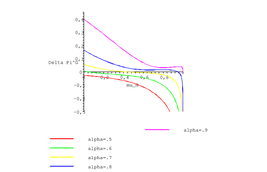
Figure 1: $\Delta\Pi^{G}(1,\mu_{G})$ as a function of $\mu_{G}$ for different values of $\alpha$.

The plot is displayed in Figure 1. This plot nicely illustrates the workings of the model. First, note that for $\alpha=.5$, $\Delta\Pi^{G}(1,\mu_{G})$ is clearly negative, so given that the Reds choose $A,$ the Greens prefer $B$ and complete segregation is an equilibrium. However, $\Delta\Pi^{G}(1,\mu_{G})$ increases with $\alpha$, such that for $\alpha>.5904\equiv\hat{\alpha}$, we have that $\Delta\Pi^{G}(1,0)>0$ and complete segregation is not an equilibrium anymore. In that case, there is a unique partial segregation equilibrium.

If $\alpha<.5904$ we have complete segregation as an equilibrium. In that case the equilibrium employment rates and the wages are characterized by the Proposition 2. Given our parameterization, employment rates are given by:

$$s_{A}^{R}=s_{B}^{G}=.95\mbox{ and }s_{B}^{R}=s_{A}^{G}=.9223.$$

Wages have a particular simple form in the case of complete segregation, being $w_{A}(1,0)=\theta\alpha$ and $w_{B}(1,0)=\theta(1-\alpha)$. Therefore, if we define the wage gap as $G(\mu_{R},\mu_{G})=1-w_{B}(\mu_{R},\mu_{G})/w_{A}(\mu_{R},\mu_{G})$, then the wage gap under complete segregation is $G(1,0)=2-1/\alpha$. Note that at $\alpha=\hat{\alpha}=.5904$, we have

$$w_{A}(1,0)=47,233\mbox{ and }w_{B}(1,0)=32,767$$

and the wage gap is thus $G(1,0)=.306$. Hence, a small employment gap of .9223 versus .95 is only compensated by a wage gap of 30 %!

It is worth elaborating on this potentially large wage gap. In equilibrium, group $R$ is completely specialized in education $A$. Therefore the wage and unemployment gap are determined by the tradeoff that workers from group $G$ are making. Choosing education $A$ gives Greens a higher wage than education $B$, but in education $B$ there would be few Green colleagues, and therefore fewer contacts. Hence, choosing $A$ would result in a lower employment rate for Green workers. Remark that this unemployment gap may be quite small compared to the wage gap. In particular, in our simulation, at $\alpha=\hat{\alpha}\equiv.5904$, the wage gap of 30 % is compensated by an employment gap of about 3 %. The reason for this tenfold magnification is risk aversion of individuals. Individuals try to avoid the (small) risk of unemployment, in which they have a payoff equal to 0, being willing to accept even major losses in income to accomplish that.

We would like to know whether an even larger wage gap can be sustained in a partial segregation equilibrium when $\alpha>\hat{\alpha}=.5904$. We therefore plot the equilibrium wages, $w_{A}(1,\mu^{\ast})$ and $w_{B}(1,\mu^{\ast})$, and equilibrium employments, $s_{A}^{R}(1,\mu^{\ast})$, $s_{B}^{R}(1,\mu^{\ast})$, $s_{A}^{G}(1,\mu^{\ast})$ and $s_{B}^{G}(1,\mu^{\ast})$, as function of $\alpha$. Remember that the equilibrium $\mu^{\ast}$ equals zero when $\alpha\leq\hat{\alpha}$, and solves $\Delta\Pi^{G}(1,\mu^{\ast})=0$ when $\alpha>\hat{\alpha}$. These plots are shown in Figures 2 and 3.

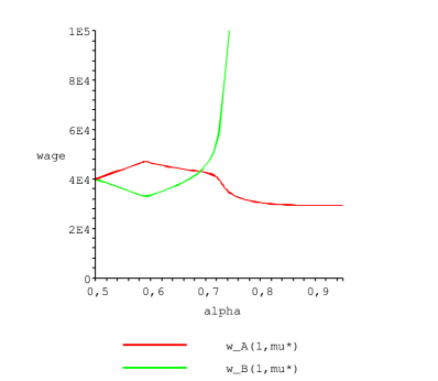
Figure 2: Equilibrium wages as function of $\alpha$.

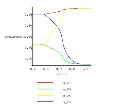
Figure 3: Equilibrium employment rates as function of $\alpha$.

The figures above embody well the qualitative implications of Propositions 2 and 3, for the chosen parameter values/ ranges. Moreover, for the chosen parameters we also observe that the wage gap $G(1,\mu^{\ast})$ is maximized at $\alpha=\hat{\alpha}$. When $\alpha$ becomes larger than $\hat{\alpha}$, the wage of $A$ declines and the wage of $B$ increases until the wage gap is reversed.

We next look at the sensitivity of $\hat{\alpha}$ with respect to the parameter choices, as we saw that at $\alpha=\hat{\alpha}$ the wage gap is maximized. We do this by computing the elasticities of $\hat{\alpha}$ and of the implied wage gap $G(1,0)$ at the chosen parameters. That is, we look at the percentage increase of $\hat{\alpha}$ and the maximum wage gap change when a parameter increases by 1 % . The elasticities are shown in columns 2 and 3 of Table 2. We note that $\hat{\alpha}$ and the implied maximum wage gap are most sensitive to $\rho\theta$, the coefficient of relative risk aversion. A 1 % increase in this coefficient leads to a 2 % increase in the maximum wage gap. On the other hand, our calibration seems least sensitive to the network parameters $c_{1}(p+\kappa)$ and $c_{1}\lambda$. The maximum wage gap seems to be close to linear with respect to $1-s_{0}$, the unemployment rate if a worker only consider direct search techniques. That is, if we chose $s_{0}=.95$ instead of $s_{0}=.90$, it would roughly halve the maximum wage gap.

5.2.2 Implications for the second-best welfare outcome

We now consider explicitly the analysis of a second-best optimum. Namely, as also briefly stated earlier in the paper, we suppose that the government (social planner) does not have the institutions to completely control $\mu_{R}$ and $\mu_{G}$, but that it is still able to stabilize a symmetric equilibrium, such that $\mu_{R}=\mu_{G}=\mu^{S}$. Should the government do this? In case the government stabilizes integration, we still impose the equilibrium condition, which is in this case symmetric. Therefore

$$\Pi_{A}^{R}(\mu^{S},\mu^{S})=\Pi_{B}^{R}(\mu^{S},\mu^{S})=\Pi_{A}^{G}(\mu^{S},\mu^{S})=\Pi_{B}^{G}(\mu^{S},\mu^{S}).$$

Hence, in the symmetric case there is complete equality. On the other hand, in the case of segregation, we consider the equilibrium allocation $(\mu_{R},\mu_{G})=(1,\mu^{\ast})$, such that Reds obtain a higher payoff than Greens. Therefore, we might face a tradeoff when assessing an integration policy. It enforces equality, but it might decrease employment.

To this purpose we plot the increase in social welfare from such an integration policy, $I=W(\mu^{S},\mu^{S})/W(1,\mu^{\ast})-1$, as function of $\alpha$. Figure 4 shows this plot.

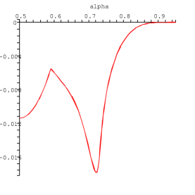
Figure 4: Percentage increase in welfare of a policy that enforces perfect integration.

We observe that $I$ is negative for all values of $\alpha$. So for the chosen parameters the integration policy is never preferred. In this world, people are better off segregated.

Our results are clear: with a utilitarian welfare function, a second best policy involves a “laissez-faire” policy, such that society becomes segregated. The intuition behind this result is twofold. First, in the case of partial segregation the equilibrium is determined by the Green workers. They trade off a benefit in wage against a loss in employment. Their individual incentives therefore already put a limit on the amount of wage inequality that can be sustained in equilibrium. Second, an integration policy would lead to lower employment rates. Or, with risk-averse individuals, the society is willing to tolerate some inequality in exchange for higher employment rates.

We finally remark that an integration policy is only beneficial when society has additional distributional concerns that are not captured by the concavity of the individual utility function. For example, consider the case of a maximin social welfare function: $W_{\min}=\min_{i}\Pi_{i}$. In the integrated case, $\mu_{R}=\mu_{G}=\mu^{S}$, everyone obtains the same payoff, whereas in the segregated case workers from group $G$ are worse off. Therefore, $W_{\min}(1,\mu^{\ast})=\Pi_{B}^{G}(1,\mu^{\ast})$ and $W_{\min}(\mu^{S},\mu^{S})=\Pi_{B}^{G}(\mu^{S},\mu^{S})$. We show a comparison of these two payoffs, $\Pi_{B}^{G}(\mu^{S},\mu^{S})/\Pi_{B}^{G}(1,\mu^{\ast})-1$, in Figure 5.

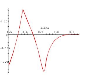
Figure 5: Percentage increase in Green workers’ payoffs of a policy enforcing perfect integration.

Observe that Greens would benefit from integration for values of $\alpha$ around $\hat{\alpha}$, where the wage gap is particularly large. In such case, strong distributional concerns would justify integration.

6 Conclusion

We have proposed a social interaction model with jobs obtained through a stochastic network of contacts, after individual career decisions had been made endogenously. Even with a tiny amount of within-social group homophily, a partial occupational segregation equilibrium, in which one group fully specializes and the other mixes over two career tracks, can be sustainable – with between-group wage and employment gaps also in line with observed gender or racial labor market disparities.

We have also analysed the implications of our model from a social planner’s perspective. In the first best social welfare optimum, segregation is socially preferred. Subject to proper calibration of our model parameters, a second best social welfare analysis supports a laissez-faire policy where society also becomes segregated, shaped by individual incentives. Both conclusions are valid in light of reasonable concavity features of the individual utility function. Our results imply that an integration policy could only be justified under distributional concerns beyond typical individual utilities; or under more complex individual preferences than those analysed in our model, for instance with direct utility derived from exposure to more diversity; and therefore that such justifications should take center stage in social integration debates.

While our model can relate empirical patterns of educational and occupational segregation to wage and employment gaps between gender or racial groups, other factors have also been documented to play a significant role. This framework should thus be seen as complement to a number of alternatives, including the classical theories of taste discrimination or rational bias by employers. In future empirical research it would be pertinent to assess the relative strength of our mechanism vis-à-vis those other channels in explaining labor market disparities.

Our model easily allows for interesting extensions. One such avenue for future research is to extend with an analysis of minority versus majority groups, by modeling the interaction between social groups of unequal sizes. Another avenue is to consider heterogeneity in productivity. The latter would allow to analyze the mismatch of workers to firms due to network effects. Finally, one could further explore whether changes in our parsimonious economy fundamentals, e.g., in the number of (initial or newly entering) occupations and in the degree of complementarity between these occupations, could alter the equilibrium towards less segregation relative to the first-best.

Appendix A Proofs

The proof of Proposition 1 uses the following lemma:

Lemma 1

Suppose Assumptions 1 and 2 hold. A stable equilibrium $(\mu_{R}^{\ast},\mu_{G}^{\ast})$ in which $0<\mu_{R}^{\ast}<1$ and $0<\mu_{G}^{\ast}<1$ does not exist.

Proof A.1.

Suppose $(\mu_{R}^{\ast},\mu_{G}^{\ast})$ is a stable equilibrium, and $\mu_{R}^{\ast}\in(0,1)$ and $\mu_{G}^{\ast}\in(0,1)$. By condition (2)

(18) $$\Pi_{A}^{R}(\mu_{R}^{\ast},\mu_{G}^{\ast})=\Pi_{B}^{R}(\mu_{R}^{\ast},\mu_{G}^{\ast})\mbox{ and }\Pi_{A}^{G}(\mu_{R}^{\ast},\mu_{G}^{\ast})=\Pi_{B}^{G}(\mu_{R}^{\ast},\mu_{G}^{\ast})$$

Substituting (8)-(9) into (18) and rewriting, these equations become

(19) $$\frac{U(w_{A}(\mu_{R}^{\ast},\mu_{G}^{\ast}))}{U(w_{B}((\mu_{R}^{\ast},\mu_{G}^{\ast}))}=\frac{s_{B}^{R}(\mu_{R}^{\ast},\mu_{G}^{\ast})}{s_{A}^{R}(\mu_{R}^{\ast},\mu_{G}^{\ast})}=\frac{s_{B}^{G}(\mu_{R}^{\ast},\mu_{G}^{\ast})}{s_{A}^{G}(\mu_{R}^{\ast},\mu_{G}^{\ast})}.$$

Since $\lambda>0$, $\mu_{R}^{\ast}>\mu_{G}^{\ast}$ implies $s_{A}^{R}>s_{A}^{G}$ and $s_{B}^{R}<s_{B}^{G}$. But this means that if $\mu_{R}^{\ast}>\mu_{G}^{\ast}$, then

$$\frac{s_{B}^{R}(\mu_{R}^{\ast},\mu_{G}^{\ast})}{s_{A}^{R}(\mu_{R}^{\ast},\mu_{G}^{\ast})}<\frac{s_{B}^{G}(\mu_{R}^{\ast},\mu_{G}^{\ast})}{s_{A}^{G}(\mu_{R}^{\ast},\mu_{G}^{\ast})}.$$

which contradicts (19). The same reasoning holds for $\mu_{R}^{\ast}<\mu_{G}^{\ast}$. Hence, it must be that $\mu_{R}^{\ast}=\mu_{G}^{\ast}$. However $(\mu_{R}^{*},\mu_{G}^{*})$ with $\mu_{R}^{*}=\mu_{G}^{*}$ cannot be a stable equilibrium. To see this, suppose that $(\mu^{*},\mu^{*})$ with $\mu^{*}\in(0,1)$ is a stable equilibrium. Hence $\Pi_{A}^{X}(\mu^{*},\mu^{*})=\Pi_{B}^{X}(\mu^{*},\mu^{*})$ for $X\in\{R,G\}$ and $\frac{\partial\Delta\Pi^{X}}{\partial\mu_{X}}<0$ at $\mu_{R}=\mu_{G}=\mu^{*}$, and det$(G(\mu^{*},\mu^{*})>0$, where $G(\mu)=D\Delta\Pi(\mu)$ is the Jacobian of $\Delta\Pi\equiv(\Delta\Pi^{R},\Delta\Pi^{G})$ with respect to $\mu\equiv(\mu_{R},\mu_{G})$. Since $\lambda>0$, it must be that

(20) $$\frac{\partial s_{A}^{X}}{\partial\mu_{X}}>\frac{\partial s_{A}^{X}}{\partial\mu_{Y}}>0$$

and

(21) $$\frac{\partial s_{B}^{X}}{\partial\mu_{X}}<\frac{\partial s_{B}^{X}}{\partial\mu_{Y}}<0$$

for $X,Y\in\{R,G\}$ and $Y\neq X$. Furthermore, if $\mu_{R}=\mu_{G}=\mu^{\ast}$, then $s_{A}^{X}=s_{A}^{Y}$, $\frac{\partial L_{A}}{\partial\mu_{X}}=\frac{\partial L_{A}}{\partial\mu_{Y}}$, $\frac{\partial L_{B}}{\partial\mu_{X}}=\frac{\partial L_{B}}{\partial\mu_{Y}}$, and therefore,

(22) $$\frac{\partial w_{A}}{\partial\mu_{X}}=\frac{\partial w_{A}}{\partial\mu_{Y}}$$

and

(23) $$\frac{\partial w_{B}}{\partial\mu_{X}}=\frac{\partial w_{B}}{\partial\mu_{Y}}.$$

By using (20)-(23) from above, together with a substitution of (8)-(9) in Assumption 2 from the main body of the paper, and a somewhat tedious but straightforward algebra, it follows that, at $\mu_{R}=\mu_{G}=\mu^{\ast}$,

$$\frac{\partial\Delta\Pi^{X}}{\partial\mu_{Y}}<\frac{\partial\Delta\Pi^{X}}{\partial\mu_{X}}<0.$$

for $X,Y\in\{R,G\}$, $X\neq Y$. But given the latest established inequalities, we can immediately see from the expression of the determinant of the Jacobian $G(\mu)=D\Delta\Pi(\mu)$ introduced above, that det$(G(\mu^{\ast},\mu^{\ast}))<0$, which contradicts the stability assumption.

PROPOSITION 1

Proof A.2.

(i) If (10) holds, then

$$\Pi_{A}^{R}(1,0)>\Pi_{B}^{R}(1,0)\mbox{ and }\Pi_{A}^{G}(1,0)<\Pi_{B}^{G}(1,0).$$

Hence, $(\mu_{R},\mu_{G})=(1,0)$ is clearly a stable equilibrium. The same is true for $(\mu_{R},\mu_{G})=(0,1)$. Lemma 1 and Assumption 2 ensure that these are the only two equilibria. (ii) If (11) is true, then

(24) $$\Pi_{A}^{G}(1,0)>\Pi_{B}^{G}(1,0).$$

Furthermore, from Assumption 1 we know that $\frac{\partial\Delta\Pi^{G}(1,\mu_{G})}{\partial\mu_{G}}<0$ for all $\mu_{G}\in[0,1]$. It follows from Assumption 1, equation (24) and continuity of $F$, $U$ and $s$, that there must be a unique $\mu^{*}$, such that

$$\Pi_{A}^{G}(1,\mu^{*})=\Pi_{B}^{G}(1,\mu^{*}).$$

Moreover, $s_{A}^{R}(1,\mu^{*})>s_{A}^{G}(1,\mu^{*})$ and $s_{B}^{G}(1,\mu^{*})>s_{B}^{R}(1,\mu^{*})$, so we have at $(\mu_{R},\mu_{G})=(1,\mu^{*})$

(25) $$\Pi_{A}^{R}>\Pi_{B}^{G}=\Pi_{A}^{G}>\Pi_{B}^{R}.$$

It is therefore clear that $(\mu_{R},\mu_{G})=(1,\mu^{*})$ is a stable equilibrium. The same is true for $(\mu_{R},\mu_{G})=(\mu^{*},1)$. To show that there is no other equilibrium, note that by (11), $\Pi_{A}^{R}(1,0)>\Pi_{B}^{R}(1,0).$ Assumption 2 then implies that $\Pi_{A}^{R}(\mu,0)>\Pi_{B}^{R}(\mu,0)$ for all $\mu\in[0,1]$. Hence, $(\mu,0)$ and, similarly, $(0,\mu)$ cannot be an equilibrium. By Lemma 1 we also know that there is no mixed equilibrium.

PROPOSITION 2

Proof A.3.

The equations follow almost directly. We have

$$s_{A}^{R}(1,0)=s_{B}^{G}(1,0)=s_{H}>s_{L}=s_{B}^{R}(1,0)=s_{A}^{G}(1,0).$$

Further, by assumption $w_{A}\geq w_{B}$ at $(\mu_{R},\mu_{G})=(1,0)$. Finally, at $(\mu_{R},\mu_{G})=(1,0)$

$$U(w_{A})s_{A}^{R}\geq U(w_{B})s_{B}^{G}\geq U(w_{A})s_{A}^{G}\geq U(w_{B})s_{B}^{R},$$

and this is equivalent to (12).

PROPOSITION 3

Proof A.4.

Consider the stable equilibrium at $(1,\mu^{\ast})$. Since it is an equilibrium we know that

$$\Pi_{A}^{G}(1,\mu^{\ast})=\Pi_{B}^{G}(1,\mu^{\ast}).$$

In the proof of Proposition 1, equation (25), we already demonstrated the inequality (14) Further, by Assumption 2 we know that $\Delta\Pi^{G}(1,\mu_{G})$ is strictly monotonically decreasing in $\mu_{G}$. (i) If $\hat{\mu}<\frac{\lambda}{2(p+\kappa+\lambda)}$, then $s_{A}^{G}(1,\hat{\mu})<s_{B}^{G}(1,\hat{\mu})$. As $w_{A}(1,\hat{\mu})=w_{B}(1,\hat{\mu})$ it must be that

$$\Pi_{A}^{G}(1,\hat{\mu})<\Pi_{B}^{G}(1,\hat{\mu}).$$

But then it also must be that $\mu^{\ast}<\hat{\mu}$. As we consider a partial segregation equilibrium, we know that $\mu^{\ast}>0$. Hence, $0<\mu^{\ast}<\hat{\mu}$ and $w_{A}(1,\hat{\mu^{\ast}})>w_{B}(1,\hat{\mu^{\ast}})$, as $w_{A}(\mu_{R},\mu_{G})$ is a decreasing function, whereas $w_{B}(\mu_{R},\mu_{G})$ is increasing. But then it also follows that $s_{A}^{G}(1,\hat{\mu^{\ast}})<s_{B}^{G}(1,\hat{\mu^{\ast}})$, since $\Pi_{A}^{G}(1,\hat{\mu^{\ast}})=\Pi_{B}^{G}(1,\hat{\mu^{\ast}})$ in equilibrium, as stated above.

(ii) If $\hat{\mu}>\frac{\lambda}{2(p+\kappa+\lambda)}$, then $s_{A}^{G}(1,\hat{\mu})>s_{B}^{G}(1,\hat{\mu})$ and $\Pi_{A}^{G}(1,\hat{\mu})<\Pi_{B}^{G}(1,\hat{\mu}).$ But then $\mu^{\ast}>\hat{\mu}$. By Assumption 1 we know that $\mu^{\ast}<1$. Hence, $\hat{\mu}<\mu^{\ast}<1$, and therefore $w_{A}(1,\hat{\mu^{\ast}})<w_{B}(1,\hat{\mu^{\ast}})$. Analous to the above, this also further implies now that $s_{A}^{G}(1,\hat{\mu^{\ast}})>s_{B}^{G}(1,\hat{\mu^{\ast}})$, since $\Pi_{A}^{G}(1,\hat{\mu^{\ast}})=\Pi_{B}^{G}(1,\hat{\mu^{\ast}})$ in equilibrium.

We next continue with the proof of Proposition 4. This proof uses the following lemma:

Lemma A.5.

Suppose that for all $x\in[0,(p+\kappa+\lambda)/2]$

(26) $$s^{\prime\prime}(x)>-\frac{4}{\lambda}\ s^{\prime}(x).$$

• If $\mu_{X}>\mu_{Y}$ for $X,Y\in\{R,G\}$, then

  (27) $$\frac{\partial L_{A}}{\partial\mu_{X}}(\mu_{R},\mu_{G})>\frac{\partial L_{A}}{\partial\mu_{Y}}(\mu_{R},\mu_{G})>0,$$

  and

  (28) $$\frac{\partial L_{B}}{\partial\mu_{Y}}(\mu_{R},\mu_{G})<\frac{\partial L_{B}}{\partial\mu_{X}}(\mu_{R},\mu_{G})<0.$$

• If $\mu_{R}=\mu_{G}=\mu$, then

  (29) $$\frac{\partial^{2}L_{A}}{(\partial\mu_{X})^{2}}(\mu,\mu)>\frac{\partial^{2}L_{A}}{\partial\mu_{X}\partial\mu_{Y}}(\mu,\mu),$$

  and

  (30) $$\frac{\partial^{2}L_{B}}{(\partial\mu_{X})^{2}}(\mu,\mu)>\frac{\partial^{2}L_{B}}{\partial\mu_{X}\partial\mu_{Y}}(\mu,\mu).$$

Proof A.6.

(i) It is easy to derive that for $X\in\{R,G\}$:

(31) $$\frac{\partial L_{A}}{\partial\mu_{X}}=\frac{1}{2}\left(s_{A}^{X}+\mu_{R}\frac{\partial s_{A}^{R}}{\partial\mu_{X}}+\mu_{G}\frac{\partial s_{A}^{G}}{\partial\mu_{X}}\right)>0$$

(32) $$\frac{\partial L_{B}}{\partial\mu_{X}}=\frac{1}{2}\left(-s_{B}^{X}+(1-\mu_{R})\frac{\partial s_{B}^{R}}{\partial\mu_{X}}+(1-\mu_{G})\frac{\partial s_{B}^{G}}{\partial\mu_{X}}\right)<0$$

at $(\mu_{R},\mu_{G})$. From (31) and (32), we find that for all $X,Y\in\{R,G\}:\partial L_{A}/\partial\mu_{X}>\partial L_{A}/\partial\mu_{Y}$ is equivalent to

(33) $$s_{A}^{X}+\mu_{X}\left(\frac{\partial s_{A}^{X}}{\partial\mu_{X}}-\frac{\partial s_{A}^{X}}{\partial\mu_{Y}}\right)>s_{A}^{Y}+\mu_{Y}\left(\frac{\partial s_{A}^{Y}}{\partial\mu_{Y}}-\frac{\partial s_{A}^{Y}}{\partial\mu_{X}}\right).$$

With the definition of $s_{A}^{X}$ in (4) we can write out

(34) $$s_{A}^{X}+\mu_{X}\left(\frac{\partial s_{A}^{X}}{\partial\mu_{X}}-\frac{\partial s_{A}^{X}}{\partial\mu_{Y}}\right)=s\left((p+\kappa)\bar{\mu}+\lambda\mu_{X}/2\right)+\frac{\mu_{X}\lambda}{2}s^{\prime}\left((p+\kappa)\bar{\mu}+\lambda\mu_{X}/2\right)$$

when $X\neq Y$. Therefore $\mu_{X}>\mu_{Y}$ is equivalent to (33), whenever (34) is strictly monotone increasing with $\mu_{X}$, where we can treat $\bar{\mu}=(\mu_{X}+\mu_{Y})/2$ as a constant. It is easy to check that this is indeed the case under condition (26). We conclude that hypothesis (27) holds whenever $\mu_{X}>\mu_{Y}$. With a similar derivation one can show that condition (26) implies (28) as well. (ii) The second derivatives of $L_{A}$ and $L_{B}$ with respect to $\mu_{X}$ and $\mu_{Y}$ are

(35) $$\frac{\partial^{2}L_{A}}{\partial\mu_{X}\partial\mu_{Y}}=\frac{1}{2}\left(\frac{\partial s_{A}^{X}}{\partial\mu_{Y}}+\frac{\partial s_{A}^{Y}}{\partial\mu_{X}}+\mu_{R}\frac{\partial^{2}s_{A}^{R}}{\partial\mu_{X}\partial\mu_{Y}}+\mu_{G}\frac{\partial^{2}s_{A}^{G}}{\partial\mu_{X}\partial\mu_{Y}}\right)$$

(36) $$\frac{\partial^{2}L_{B}}{\partial\mu_{X}\partial\mu_{Y}}=\frac{1}{2}\left(-\frac{\partial s_{B}^{X}}{\partial\mu_{Y}}-\frac{\partial s_{B}^{Y}}{\partial\mu_{X}}+(1-\mu_{R})\frac{\partial^{2}s_{B}^{R}}{\partial\mu_{X}\partial\mu_{Y}}+(1-\mu_{G})\frac{\partial^{2}s_{B}^{G}}{\partial\mu_{X}\partial\mu_{Y}}\right).$$

Taking the second derivatives of $s_{A}^{X}$, evaluating at $\mu_{R}=\mu_{G}=\mu$ and reordering, we get that (29) is equivalent to

(37) $$s^{\prime\prime}((p+\kappa+\lambda)\mu/2)<-\frac{4}{\lambda\mu}s^{\prime}((p+\kappa+\lambda)\mu/2).$$

Inequality (37) clearly holds if condition (26) holds, which proves (29). In a similar fashion, (26) implies (30)

PROPOSITION 4

Proof A.7.

Suppose that $W(\mu_{R},\mu_{G})$ is maximized at $(\mu_{R},\mu_{G})=(\tilde{\mu}_{R},\tilde{\mu}_{G})$, where $\tilde{\mu}_{R}\in(0,1)$ and $\tilde{\mu}_{G}\in(0,1)$. Define $c\equiv L_{A}(\tilde{\mu}_{R},\tilde{\mu}_{G})/L_{B}(\tilde{\mu}_{R},\tilde{\mu}_{G})$, and consider the constrained maximization problem:

(38) $$\max_{\mu_{R}\in[0,1],\mu_{G}\in[0,1]}W(\mu_{R},\mu_{G})\mbox{ s.t. }L_{A}(\mu_{R},\mu_{G})=cL_{B}(\mu_{R},\mu_{G}).$$

Because by definition of $c$, the solution $(\tilde{\mu}_{R},\tilde{\mu}_{G})$ satisfies the restriction

(39) $$g(\mu_{R},\mu_{G})=cL_{B}(\mu_{R},\mu_{G})-L_{A}(\mu_{R},\mu_{G})=0,$$

it actually solves the maximization problem (38). Define the feasible set $C=\{\mu_{R}\in[0,1],\mu_{G}\in[0,1]|g(\mu_{R},\mu_{G})=0\}$. By the assumption of constant returns to scale, we have that for all $(\mu_{R},\mu_{G})\in C$: $w_{A}(\mu_{R},\mu_{G})$ and $w_{B}(\mu_{R},\mu_{G})$ are constant, and therefore, at all $(\mu_{R},\mu_{G})\in C$, the welfare function (16) can be written as

$$W(\mu_{R},\mu_{G})=L_{A}(\mu_{R},\mu_{G})(U(\overline{w_{A}})+U(\overline{w_{B}})/c),$$

which is monotone increasing with $L_{A}(\mu_{R},\mu_{G})$. Therefore, the solution $(\tilde{\mu}_{R},\tilde{\mu}_{G})$ also solves the following maximization problem:

(40) $$\max_{\mu_{R}\in[0,1],\mu_{G}\in[0,1]}L_{A}(\mu_{R},\mu_{G})\mbox{ s.t. }L_{A}(\mu_{R},\mu_{G})=cL_{B}(\mu_{R},\mu_{G}).$$

We verify that $(\tilde{\mu}_{R},\tilde{\mu}_{G})$ indeed satisfy the first- and second-order conditions of problem (40). The Lagrangian is given by

$$\mathcal{L}(\mu_{R},\mu_{G},\psi)=(1-\psi)L_{A}(\mu_{R},\mu_{G})+\psi cL_{B}(\mu_{R},\mu_{G}).$$

Since $(\tilde{\mu}_{R},\tilde{\mu}_{G})$ is supposed to be interior, the following first order constraints should hold:

(41) $$\frac{\partial\mathcal{L}}{\partial\mu_{R}}(\tilde{\mu}_{R},\tilde{\mu}_{G},\psi)=(1-\psi)\frac{\partial L_{A}}{\partial\mu_{R}}(\tilde{\mu}_{R},\tilde{\mu}_{G})+\psi c\frac{\partial L_{B}}{\partial\mu_{R}}(\tilde{\mu}_{R},\tilde{\mu}_{G}) =0$$

(42) $$\frac{\partial\mathcal{L}}{\partial\mu_{G}}(\tilde{\mu}_{R},\tilde{\mu}_{G},\psi)=(1-\psi)\frac{\partial L_{A}}{\partial\mu_{G}}(\tilde{\mu}_{R},\tilde{\mu}_{G})+\psi c\frac{\partial L_{B}}{\partial\mu_{G}}(\tilde{\mu}_{R},\tilde{\mu}_{G}) =0.$$

The first part of Lemma A.5 implies that $\psi\in(0,1)$ and that under condition (26): $\mu_{R}>\mu_{G}$ if and only if $\partial\mathcal{L}/\partial\mu_{R}>\partial\mathcal{L}/\partial\mu_{G}$. Therefore, condition (26) and the first-order conditions imply that $\tilde{\mu}_{R}=\tilde{\mu}_{G}\equiv\tilde{\mu}$. Since $\tilde{\mu}_{R}=\tilde{\mu}_{G}$ defines a unique point in $C$, the second-order condition should hold at $\tilde{\mu}_{R}=\tilde{\mu}_{G}$, which says that the Hessian of the Lagrangian with respect to $(\mu_{R},\mu_{G})$ evaluated at the social optimum, $D_{\mu_{R},\mu_{G}}^{2}\mathcal{L}(\tilde{\mu},\tilde{\mu},\psi)$, is negative definite on the subspace $\{z_{R},z_{G}|z_{R}(\partial g/\partial\mu_{R})+z_{G}(\partial g/\partial\mu_{G})=0\}$. The second order condition is thus that at $(\mu_{R},\mu_{G})=(\tilde{\mu},\tilde{\mu})$:

(43) $$2\frac{\partial g}{\partial\mu_{R}}\frac{\partial g}{\partial\mu_{G}}\frac{\partial^{2}\mathcal{L}}{\partial\mu_{R}\partial\mu_{G}}-\left(\frac{\partial g}{\partial\mu_{R}}\right)^{2}\frac{\partial^{2}\mathcal{L}}{(\partial\mu_{G})^{2}}-\left(\frac{\partial g}{\partial\mu_{G}}\right)^{2}\frac{\partial^{2}\mathcal{L}}{(\partial\mu_{R})^{2}}>0.$$

Because $\frac{\partial g}{\partial\mu_{R}}(\tilde{\mu},\tilde{\mu})=\frac{\partial g}{\partial\mu_{G}}(\tilde{\mu},\tilde{\mu}),$ and $\frac{\partial^{2}\mathcal{L}}{(\partial\mu_{G})^{2}}(\tilde{\mu},\tilde{\mu})=\frac{\partial^{2}\mathcal{L}}{(\partial\mu_{R})^{2}}(\tilde{\mu},\tilde{\mu}),$ the second order condition (43) simplifies to $\frac{\partial^{2}\mathcal{L}}{\partial\mu_{R}\partial\mu_{G}}(\tilde{\mu},\tilde{\mu})>\frac{\partial^{2}\mathcal{L}}{(\partial\mu_{R})^{2}}(\tilde{\mu},\tilde{\mu}),$ or equivalently

(44) $$(1-\psi)\frac{\partial^{2}L_{A}}{\partial\mu_{R}\partial\mu_{G}}(\tilde{\mu},\tilde{\mu})+\psi c\frac{\partial^{2}L_{B}}{\partial\mu_{R}\partial\mu_{G}}(\tilde{\mu},\tilde{\mu})>(1-\psi)\frac{\partial^{2}L_{A}}{(\partial\mu_{R})^{2}}(\tilde{\mu},\tilde{\mu})+\psi c\frac{\partial^{2}L_{B}}{(\partial\mu_{R})^{2}}(\tilde{\mu},\tilde{\mu}).$$

By the second part of Lemma A.5, inequality (44) cannot hold under condition (26). Therefore we have a contradiction and the non-segregation allocation $(\tilde{\mu}_{R},\tilde{\mu}_{G})$ cannot be a social optimum. Since a social optimum exists by continuity of $W$ and compactness of $[0,1]^{2}$, the social optimum necessarily has to involve complete or partial segregation.

References

- Albelda (1986) Albelda, R.P. 1986. Occupational Segregation by Race and Gender: 1958–1981. Industrial and Labor Relations Review 39 404-411.
- Alesina and La Ferrara (2000) Alesina, A. and E. La Ferrara. 2000. Participation in Heterogeneous Communities. Quarterly Journal of Economics 115 847-904.
- Alesina and La Ferrara (2002) Alesina, A. and E. La Ferrara. 2002. Who Trusts Others?. Journal of Public Economics 85 207-234.
- Altonji and Blank (1999) Altonji, J.G. and R.M. Blank. 1999. Race and Gender in the Labor Market. in O. Ashenfelter and D. Card (eds). Handbook of Labor Economics 3 3143-3259.
- Arrow (1998) Arrow, K. 1998. What Has Economics to Say about Racial Discrimination?. Journal of Economic Perspectives 12 91-100.
- Bayard et al (2003) Bayard, K., J. Hellerstein, D. Neumark, and K. Troske. 2003. New Evidence on Sex Segregation and Sex Differences in Wages from Matched Employee-Employer Data. Journal of Labor Economics 21(4) 887-922.
- Bayer et al (2008) Bayer, P., S. L. Ross, and G. Topa. 2008. Place of Work and Place of Residence: Informal Hiring Networks and Labor Market Outcomes. Journal of Political Economy 116(6) 1150-1196.
- Beaman et al (2018) Beaman, L., N. Keleher, and J. Magruder. 2018. Do job networks disadvantage women? Evidence from a recruitment experiment in Malawi. Journal of Labor Economics 36(1) 121-157.
- Beller (1982) Beller, A. 1982. Occupational Segregation by Sex: Determinants and Changes. Journal of Human Resources 17 371-392.
- Benabou (1993) Benabou, R. 1993. Workings of a City: Location, Education, and Production. Quarterly Journal of Economics 108 619-652.
- Bertrand (2011) Bertrand, M. 2011. New Perspectives on Gender. in: O. Ashenfelter and D. Card (eds). Handbook of Labor Economics 4B 1545-1592.
- Bewley (1999) Bewley, T.F. 1999. Why Wages Don’t Fall During a Recession, Harvard University Press.
- Blau and Kahn (2000) Blau, F.D. and L.M. Kahn. 2000. Gender Differences in Pay. Journal of Economic Perspectives 14(4) 75-99.
- Blau and Kahn (2006) Blau, F.D. and L.M. Kahn. 2006. The U.S. Gender Pay Gap in the 1990s: Slowing Convergence. Industrial and Labor Relations Review 60(1) 45-65.
- Blau and Kahn (2017) Blau, F.D. and L.M. Kahn. 2017. The Gender Wage Gap: Extent, Trends, and Explanations. Journal of Economic Literature 55(3) 789-865.
- Bolte et al (2022) Bolte, L, N. Immorlica and M. Jackson. 2022. The Role of Referrals in Inequality, Immobility, and Inneficiency in Labor Markets. mimeo at https://papers.ssrn.com/sol3/papers.cfm?abstractid=3512293.
- Bramoullé and Saint-Paul (2010) Bramoullé, Y. and G. Saint-Paul. 2010. Social Networks and Labor Market Transitions. Labour Economics 17 188-195.
- Brass (1985) Brass, D.J. 1985. Men’s and Women’s Networks: A Study of Interaction Patterns and Influence in an Organization. Academy of Management Journal 28 327-343.
- Brown et al (2016) Brown, M., E. Setren, and G. Topa. 2016. Do informal referrals lead to better matches? Evidence from a firm’s employee referral system. Journal of Labor Economics 28(1) 161-209.
- Burks et al (2015) Burks, S. V., B. Cowgill, M. Hoffman, and M. Housman. 2015. The Value of Hiring through Employee Referrals. Quarterly Journal of Economics 130(2) 805-839.
- Burt (1992) Burt, R. S. 1992. Structural Holes: The Social Structure of Competition. Harvard University Press.
- Burt (1998) Burt, R. S. 1998. The Gender of Social Capital. Rationality and Society 10(1) 5-46.
- Calvo (2004) Calvó-Armengol, A. 2004. Job Contact Networks. Journal of Economic Theory 115 191-206.
- Calvo and Jackson (2004) Calvó-Armengol, A. and M.O. Jackson. 2004. The Effects of Social Networks on Employment and Inequality. American Economic Review 94 426-454.
- Calvo and Jackson (2007) Calvó-Armengol, A. and M.O. Jackson. 2007. Networks in Labor Markets: Wage and Employment Dynamics and Inequality. Journal of Economic Theory. 132 27-46.
- Calvo and Zenou (2005) Calvó-Armengol, A. and Y. Zenou. 2005. Job Matching, Social Network and Word-of-Mouth Communication. Journal of Urban Economics. 57 500-522.
- Charles and Grusky (2004) Charles, M. and D.B. Grusky. 2004. Occupational Ghettos: The Worldwide Segregation of Women and Men. Stanford University Press.
- Cohen and Einav (2007) Cohen, A. and L. Einav. 2007. Estimating Risk Preferences from Deductible Choices. American Economic Review. 97 745-788.
- Coleman (1958) Coleman, J. S. 1958. Relational Analysis: The Study of Social Organizations with Survey Methods. Human Organization 17(4) 28-36.
- Cooper and John (1988) Cooper, R. and A. John. Coordination Failures in Keynesian Models. Quarterly Journal of Economics 103(3) 441-463.
- Cotter et al (2004) Cotter, D.A, J. M. Hermsen and R. Vanneman. 2004. Gender Inequality at Work. Russell Sage Foundation.
- Currarini et al (2009) Currarini, S., M.O. Jackson and P. Pin. 2009. An Economic Model of Friendship: Homophily, Minorities and Segregation. Econometrica 77 1003-1045.
- Datcher (1983) Datcher, L. 1983. The Impact of Informal Networks on Quit Behavior. Review of Economics and Statistics 65 491-495.
- Datcher Loury (2006) Datcher Loury, L. 2006. Some Contacts Are More Equal than Others: Informal Networks, Job Tenure, and Wages. Journal of Labor Economics 24 299-318.
- Diamond (1982) Diamond, P. 1982. Aggregate Demand Management in Search Equilibrium. Journal of Political Economy 905 881-894.
- Doeringer and Piore (1971) Doeringer P.B. and M.J. Piore. 1971. Internal Labor Markets and Manpower Analysis. Lexington Books.
- EIGE (2020) European Institute for Gender Equality (EIGE). 2020. Gender Equality Index 2020. Digitalisation and the Future of Work. Luxembourg: Publications Office of the European Union.
- England et al (2020) England, P., A. Levine, and E. Mishel. 2020. Progress toward gender equality in the United States has slowed or stalled. Proceedings of the National Academy of Sciences 117(13) 6990-6997.
- Fernandez and Sosa (2005) Fernandez, R.M. and M.L. Sosa. 2005. Gendering the job: Networks and Recruitment at a Call Centre. American Journal of Sociology 111 859-904.
- Gertner (1993) Gertner, R. 1993. Game Shows and Economic Behavior: Risk Taking on “Card Sharks”. Quarterly Journal of Economics 108 507-521.
- Goyal (2007) Goyal, S. 2007. Connections: An Introduction to the Economics of Networks. Princeton University Press.
- Goyal (2016) Goyal, S. 2016. Networks in Economics: A Perspective on the Literature. The Oxford Handbook of the Economics of Networks.
- Goldin (2014) Goldin, C. 2014. A Grand Gender Convergence: Its Last Chapter. American Economic Review 104(4) 1091-1119.
- Goldin and Katz (2011) Goldin, C. and L.F. Katz. 2011. The Cost of Work Place Flexibility of High Powered Professionals. The Annals of the American Academy 638(1) 45-64.
- Goldin and Katz (2016) Goldin, C. and L. F. Katz. 2016. The Most Egalitarian Profession: Pharmacy and the Evolution of a Family–Friendly Occupation. Journal of Labor Economics 34(3) 705-746.
- Graham et al (2010) Graham, B.S., G.W. Imbens, and G. Ridder. 2010. Measuring the Effects of Segregation in the Presence of Social Spillovers: A Nonparametric Approach. NBER Working Paper No. 16499.
- Granovetter (1973) Granovetter, M.S. 1973. The Strength of Weak Ties. American Journal of Sociology 78 1360-1380.
- Granovetter (1995) Granovetter, M.S. 1995. Getting a Job: A Study of Contacts and Careers (2nd). University of Chicago Press.
- Granovetter (2002) Granovetter, M.S. 2002. A Theoretical Agenda for Economic Sociology. in Guillén, Collins, England and Meyer (eds). The New Economic Sociology: Developments in an Emerging Field. Russell Sage Found.
- Hederos et al (2022) Hederos, K., A. Sandberg, L. Kvissberg, and E. Polano. 2022. Gender Homophily in Job Referrals: Evidence From a Field Study Among University Students. mimeo at http://dx.doi.org/10.2139/ssrn.4103637.
- Hellerstein et al (2011) Hellerstein, J. K., M. McInerney, and D. Neumark. 2011. Neighbors and Coworkers: The Importance of Residential Labor Market Networks. Journal of Labor Economics 29(4) 659-695.
- Holzer (1987) Holzer, H.J. 1987. ”Informal Job Search and Black Youth Unemployment. American Economic Review. 77 446-452.
- Ibarra (1992) Ibarra, H. 1992. Homophily and Differential Returns: Sex Differences in Network Structure and Access in an Advertising Firm. Administrative Science Quarterly 37 422-447.
- Ioannides and Datcher Loury (2004) Ioannides, Y.M. and L. Datcher Loury. 2004. Job Information Networks, Neighborhood Effects, and Inequality. Journal of Economic Literature 42 1056-1093.
- Ioannides and Soutevent (2006) Ioannides, Y.M. and A.R. Soetevent. 2006. Wages and Employment in a Random Social Network with Arbitrary Degree Distribution. American Economic Review P and P 96 270-274.
- Jackson (2008) Jackson, M. 2008. Social and Economic Networks. Princeton University Press.
- Jackson (2022) Jackson, M. 2022. Inequality’s Economic and Social Roots: the Role of Social Networks and Homophily. mimeo at https://ssrn.com/abstract=3795626.
- Kahneman and Tversky (1979) Kahneman, D., and A. Tversky. 1979. Prospect Theory: An Analysis of Decision under Risk. Econometrica 47 263-292.
- King (1992) King, M.C. 1992. The Evolution of Occupational Segregation by Race and Gender, 1940-1988. Monthly Labor Review 115 30-36.
- Lazarsfeld and Merton (1954) Lazarsfeld, P.F. and R.K. Merton. 1954. ”Friendship as Social Process: A Substantive and Methodological Analysis,” in Berger, Abel and Page (eds). Freedom and Control in Modern Society. Van Nostrand
- Lindenlaub and Prummer (2021) Lindenlaub, I. and A. Prummer. 2021. Network Structure and Performance. Economic Journal 131 851-898.
- Macpherson and Hirsch (1995) Macpherson, D.A. and B.T. Hirsch. 1995. Wages and Gender Composition: Why Do Women’s Jobs Pay Less?. Journal of Labor Economics 13(3) 426-471.
- Mailath et al (2000) Mailath, G. J., L. Samuelson, and A. Shaked. 2000. Endogenous Inequality in Integrated Labor Markets with Two-Sided Search. American Economic Review 90(1) 46-72.
- Manning and Swaffield (2008) Manning, A. and J. Swaffield. 2008. The Gender Gap in Early-Career Wage Growth. Economic Journal 118 987-1024.
- Marsden (1987) Marsden, P.V. 1987. Core Discussion Networks of Americans. American Sociological Review 52 122-131.
- Marsden (1988) Marsden, P.V. 1988. Homogeneity in Confiding Relations. Social Networks 10 57-76.
- Mayer and Puller (2008) Mayer, A. and S.L. Puller. 2008. The Old Boy (and Girl) Network: Social Network Formation on University Campuses. Journal of Public Economics 92 329-347.
- McPherson et al (2001) McPherson, M., L. Smith-Lovin and J.M. Cook. 2001. Birds of a Feather: Homophily in Social Networks. Annual Review of Sociology 27 415-444.
- Mengel (2020) Mengel, F. 2020. Gender differences in networking. Economic Journal 130 1842-1873.
- Metrick (1995) Metrick, A. 1995. A Natural Experiment in ”Jeopardy!”. American Economic Review 85 240-253.
- Montgomery (1991) Montgomery, J.D. 1991. Social Networks and Labor-Market Outcomes: Toward an Economic Analysis. American Economic Review 81 1408-1418.
- Montgomery (1992) Montgomery, J.D. 1992. Social Networks and Persistent Inequality in the Labor Market. mimeo, available at https://www.sebastianbuhai.com/papers/publications/aux/montgomery1992.pdf.
- Okafor (2020) Okafor, C.O. 2020. All Things Equal? Social Networks as a Mechanism for Discrimination. mimeo, available at https://arxiv.org/abs/2006.15988.
- Padavic and Reskin (2002) Padavic, B.F. and I. Reskin. 2002. Women and Men at Work(2nd). Pine Forge Press.
- Pettit and Hook (2005) Pettit, B. and J. Hook. 2005. The Structure of Women’s Employment in Comparative Perspective. Social Forces 84 779-801.
- Rees (1966) Rees, A. 1966. Information Networks in Labor Markets. American Economic Review 56 559-566.
- Shrum et al (1988) Shrum, W., N.H. Cheek and S.M. Hunter. 1988. Friendship in School: Gender and Racial Homophily. Sociology of Education 61 227-239.
- Simon and Warner (1992) Simon, C.J. and J.T. Warner. 1992. Matchmaker, Matchmaker: The Effect of Old Boy Networks on Job Match Quality, Earnings, and Tenure. Journal of Labor Economics 10 306-330.
- Sørensen (2004) Sørensen, J.B. 2004. The Organizational Demography of Racial Employment Segregation. American Journal of Sociology 110 626-671.
- Tampubolon (2005) Tampubolon, G. 2005. Fluxes and Constants in the Dynamics of Friendships. ESRC Working Paper No. 25.
- Topa (2001) Topa, G. 2001. Social Interactions, Local Spillovers and Unemployment. Review of Economic Studies 68 261-295.
- Topa (2011) Topa, G. 2011. Labor Markets and Referrals. Handbook of Social Economics. Elsevier North Holland.
- Weeden and Sørensen (2004) Weeden, K.A. and J.B. Sørensen. 2004. Two-Dimensional Models of Sex Segregation: Industries and Occupations. in – the above cited – Charles and Grusky (2004), 245-294.
- Zeltzer (2020) Zeltzer, D. 2020. Gender Homophily in Referral Networks: Consequences for the Medicare Physician Earnings Gap. American Economic Journal: Applied Economics 12(2) 169-197.