Space of Functions Computed by Deep-Layered Machines

Abstract

We study the space of functions computed by random-layered machines, including deep neural networks and Boolean circuits. Investigating the distribution of Boolean functions computed on the recurrent and layer-dependent architectures, we find that it is the same in both models. Depending on the initial conditions and computing elements used, we characterize the space of functions computed at the large depth limit and show that the macroscopic entropy of Boolean functions is either monotonically increasing or decreasing with the growing depth.

Deep-layered machines comprise multiple consecutive layers of basic computing elements aimed at representing an arbitrary function, where the first and final layers represent its input and output arguments, respectively. Notable examples include deep neural networks (DNNs) composed of perceptrons LeCun2015 and Boolean circuits constructed from logical gates ODonnell2014 . Being universal approximators Hornik1989 ; Poole2016 , DNNs have been successfully employed in different machine learning applications LeCun2015 . Similarly, Boolean circuits can compute any Boolean function even when constructed from a single gate Nisan2008 .

While the majority of DNN research focuses on their application in carrying out various learning tasks, it is equally important to establish the space of functions they typically represent for a given architecture and the computing elements used. One way to address such a generic study is to consider a random ensemble of DNNs. The study of random neural networks using methods of statistical physics has played an important role in understanding their typical properties for storage capacity and generalization ability Engel2001 ; Saad1998 and properties of energy-based Agliari2012 ; Huang2015 ; Gabrie2015 ; Mezard2017 ; Barra2018 and associative memory models Hopfield1982 ; Hertz1991 , as well as the links between energy-based models and feed-forward layered machines Hopfield1987 . In parallel, there have been theoretical studies within the computer science community of the range of Boolean functions generated by random Boolean circuits Savicky1990 ; Brodsky2005 . Both the DNNs and the Boolean circuits share common basic properties.

Characterizing the space of functions computed by random-layered machines is of great importance, since it sheds light on their approximation and generalization properties. However, it is also highly challenging due to the inherent recursiveness of computation and randomness in their architecture and/or computing elements. Existing theoretical studies of the function space of deep-layered machines are mostly based on the mean field approach, which allows for a sensitivity analysis of the functions realized by deep-layered machines due to input or parameter perturbations Poole2016 ; Lee2018 ; BoLi2018 ; BoLi2020 .

To gain a complete and detailed understanding of the function space, we develop a path-integral formalism that directly examines individual functions computed. This is carried out by processing all possible input configurations simultaneously and the corresponding outputs. For simplicity, we always consider Boolean functions with binary input and output variables.

The main contribution of this Letter is in providing a detailed understanding of the distribution of Boolean functions computed at each layer. It points to the equivalence between recurrent and layer-dependent architectures, and consequently to the potential significant reduction in the number of trained free variables. Additionally, the complexity of Boolean functions implemented measured by their entropy, which depends on the number of layers and computing elements used, exhibits a rapid simplification when rectified linear unit (ReLU) components are employed, which arguably explains their generalization successes.

Framework.––The layered machines considered consist of $L+1$ layers, each with $N$ nodes. Node $i$ at layer $l$ is connected to the set of nodes $\{i_{1},i_{2},...,i_{k}\}$ of layer $l-1$; its activity is determined by the gate $\alpha_{i}^{l}$, computing a function of $k$ inputs, according to the propagation rule

$$P(S_{i}^{l}|\vec{S}^{l-1})=\delta\big{[}S_{i}^{l},\alpha_{i}^{l}(S_{i_{1}}^{l-1},S_{i_{2}}^{l-1},...,S_{i_{k}}^{l-1})\big{]},$$ (1)

where $\delta$ is the Dirac or Kronecker delta function, depending on the domain of $S_{i}^{l}$. The probabilistic form of Eq. (1) adopted here is convenient for the generating functional analysis and inclusion of noise Mozeika2009 ; BoLi2018 . We primarily consider two structures here: (i) densely connected models where $k=N$ and node $i$ is connected to all nodes from the previous layer––one such example is the fully connected neural network with $S_{i}^{l}=\alpha^{l}(H_{i}^{l})$, where $H_{i}^{l}=\sum_{j=1}^{N}W_{j}^{l}S_{j}^{l-1}/\sqrt{N}+b_{i}^{l}$ is the preactivation field and $\alpha^{l}$ is the activation function at layer $l$, (we will mainly focus on the case $b_{i}^{l}=0$; the effect of nonzero bias is discussed in Mozeika2020sup ); (ii) sparsely connected models where $k\in O(N^{0})$––examples include the sparse neural networks and layered Boolean circuits where $\alpha_{i}^{l}$ is a Boolean gate with $k$ inputs, e.g., majority gate.

Consider a binary input vector $\vec{s}=(s_{1},\ldots,s_{n})\in\{-1,1\}^{n}$, which is fed to the initial layer $l=0$. To accommodate a broader set of functions, we also consider an augmented input vector, e.g., (i) $\vec{S}^{I}=(\vec{s},1)$, which is equivalent to adding a bias variable in the context of neural networks; (ii) $\vec{S}^{I}=(\vec{s},-\vec{s},1,-1)$, which has been used to construct all Boolean functions Savicky1990 . Each node $i$ at layer $0$ points to a randomly chosen element of $\vec{S}^{I}$ such that

$$P^{0}(\vec{S}^{0}|\vec{s})=\prod_{i=1}^{N}P^{0}\big{[}S_{i}^{0}|S_{n_{i}}^{I}(\vec{s})\big{]}=\prod_{i=1}^{N}\delta\big{[}S_{i}^{0},S_{n_{i}}^{I}(\vec{s})\big{]},$$ (2)

where $n_{i}=1,...,|\vec{S}^{I}|$ is an index chosen from the flat distribution $P(n_{i})=1/|\vec{S}^{I}|$.

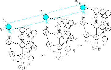
Figure 1: A deep-layered machine computing all possible $2^{n}$ inputs. The direction of computation is from bottom to top. The binary string $\bm{S}^{L}\in\{-1,1\}^{2^{n}}$ represents the Boolean function computed on the blue nodes of the output layer $L$. The augmented vector $\vec{S}^{I}=(\vec{s},1)$ is used as an example of input here. The constant $1$ is represented by the dashed circle.

The computation of the layered machine is governed by the propagator $P(\vec{S}^{L}|\vec{s})=\sum_{\vec{S}^{L-1}\cdots\vec{S}^{0}}P(\vec{S}^{0}|\vec{s})\prod_{l=1}^{L}P(\vec{S}^{l}|\vec{S}^{l-1})$, where each node at layer $L$ computes a Boolean function $\{-1,1\}^{n}\to\{-1,1\}$. When the gates $\alpha_{i}^{l}$ or the network topology are random, then the layered machine can be viewed as a disordered dynamical system with quenched disorder Mozeika2009 ; BoLi2018 . To probe the functions being computed, we consider the simultaneous layer propagation of all possible inputs $\vec{s}_{\gamma}\in\{-1,1\}^{n}$, labeled by $\gamma=1,\ldots,2^{n}$ governed by the product propagator $\prod_{\gamma=1}^{2^{n}}P(\vec{S}_{\gamma}^{L}|\vec{s}_{\gamma})$. The binary string $\bm{S}_{i}^{L}\in\{-1,1\}^{2^{n}}$ represents the Boolean function computed at node $i$ at layer $L$, as illustrated in Fig. 1. Note that we use the vector notation $\vec{S}^{l}=(S_{1}^{l},...,S_{i}^{l},...,S_{N}^{l})$ and $\bm{S}_{i}^{l}=(S_{i,1}^{l},...,S_{i,\gamma}^{l},...,S_{i,2^{n}}^{l})$ to represent the states and functions, respectively. Using the above formalism, the distribution of Boolean functions $\bm{f}$ computed on the final layer is given by

$$P_{N}^{L}(\bm{f}) = \frac{1}{N}\sum_{i=1}^{N}\left\langle\prod_{\gamma=1}^{2^{n}}\delta\left(f_{\gamma},S_{i,\gamma}^{L}\right)\right\rangle,$$ (3)

where components of $\bm{f}$ satisfy $f_{\gamma}=f(\vec{s}_{\gamma})$, and angular brackets represent the average generated by $\prod_{\gamma=1}^{2^{n}}P(\vec{S}_{\gamma}^{L}|\vec{s}_{\gamma})$. To compute $P_{N}^{L}(\bm{f})$ and averages of other macroscopic observables, which are expected to be self-averaging for $N\to\infty$ Mezard1987 , we introduce the disorder-averaged generating functional (GF) $\overline{\Gamma[\{\psi_{i,\gamma}^{l}\}]}=\overline{\sum_{\{\vec{S}_{\gamma}^{l}\}}\prod_{\gamma}P(\vec{S}_{\gamma}^{0}|\vec{S}_{\gamma}^{I})\prod_{l}P(\vec{S}_{\gamma}^{l}|\vec{S}_{\gamma}^{l-1})e^{-\mathrm{i}\sum_{i}\psi_{i,\gamma}^{l}S_{i,\gamma}^{l}}}$, where the overline denotes an average over the quenched disorder. To keep the presentation concise, we outline the GF formalism only for DNNs in the following and refer the reader to Mozeika2020sup for the details of the derivation used in Boolean circuits.

Layer-dependent and recurrent architectures.––We focus on two different architectures: layer-dependent architectures, where the gates and/or connections are different from layer to layer, and recurrent, where the gates and connections are shared across all layers. Both architectures represent feed-forward machines that implement input-output mappings.

Specifically, we assume that the weights $W_{ij}^{l}$ in fully connected DNNs with layer-dependent architectures are independent Gaussian random variables sampled from $\mathcal{N}(0,\sigma^{2})$. In DNNs with recurrent architectures, the weights are sampled once and are shared among layers, i.e. $W_{ij}^{l+1}=W_{ij}^{l}$. We apply the sign activation function in the final layer, i.e. $\alpha^{L}(h_{i}^{L})=\mathrm{sgn}(h_{i}^{L})$, to ensure that the output of the DNN is Boolean.

We first outline the derivation for fully connected recurrent architectures. It is sufficient to characterize the disorder-averaged GF by introducing cross-layer overlaps $q_{\gamma\gamma^{\prime}}^{l,l^{\prime}}=(1/N)\sum_{i}\overline{\langle S_{i,\gamma}^{l}S_{i,\gamma^{\prime}}^{l^{\prime}}\rangle}$ as order parameters and the corresponding conjugate order parameter $Q_{\gamma\gamma^{\prime}}^{l,l^{\prime}}$, which leads to a saddle-point integral $\overline{\Gamma}=\int\{\mathrm{d}\bm{q}\,\mathrm{d}\bm{Q}\}\mathrm{e}^{N\Psi[\bm{q},\bm{Q}]}$ with the potential Mozeika2020sup

$$\Psi\!=\mathrm{i}\mathrm{Tr}\left\{\bm{q}\,\bm{Q}\right\}+\sum_{m=1}^{|\vec{S}^{I}|}P(m)\ln\sum_{\bm{S}}\!\int\!\mathrm{d}\bm{H}\mathcal{M}_{m}[\bm{H},\bm{S}],$$ (4)

where $\mathcal{M}_{m}[\bm{H},\bm{S}]$ is an effective single-site measure

$$\mathcal{M}_{m} = \mathrm{e}^{-\mathrm{i}\sum_{l,\gamma}\psi_{\gamma}^{l}S_{\gamma}^{l}-\mathrm{i}\sum_{ll^{\prime},\gamma\gamma^{\prime}}Q_{\gamma\gamma^{\prime}}^{l,l^{\prime}}S_{\gamma}^{l}S_{\gamma^{\prime}}^{l^{\prime}}}$$

$$\times\mathcal{N}\big{(}\bm{H}|\bm{0},\bm{C}\big{)}\prod_{\gamma=1}^{2^{n}}P^{0}(S_{\gamma}^{0}|S_{m,\gamma}^{I})\prod_{l=1}^{L}\delta\big{[}S_{\gamma}^{l},\alpha^{l}(h_{\gamma}^{l})\big{]}.$$

Due to weight sharing, the preactivation fields $\bm{H}=(\bm{h}^{1},\ldots,\bm{h}^{L})$, where $\bm{h}^{l}\in\mathbb{R}^{2^{n}}$, are governed by the Gaussian distribution $\mathcal{N}\left(\bm{H}|\bm{0},\bm{C}\right)$ and correlated across layers with covariance $[\bm{C}\,]_{\gamma\gamma^{\prime}}^{l,l^{\prime}}=\sigma^{2}q_{\gamma\gamma^{\prime}}^{l-1,l^{\prime}-1}$. Setting $\psi_{\gamma}^{l}$ to zero and differentiating $\Psi$ with respect to $\{q_{\gamma\gamma^{\prime}}^{l,l^{\prime}},Q_{\gamma\gamma^{\prime}}^{l,l^{\prime}}\}$ yields the saddle point of the potential $\Psi$ dominating $\overline{\Gamma}$ for $N\rightarrow\infty$, at which the conjugate order parameters $Q_{\gamma\gamma^{\prime}}^{l,l^{\prime}}$ vanish Mozeika2020sup , leading to

$$q_{\gamma\gamma^{\prime}}^{l,l^{\prime}}=\begin{cases}\sum_{m}P(m)\big{\langle}S_{\gamma}^{l}S_{\gamma^{\prime}}^{0}\big{\rangle}_{\mathcal{M}_{m}},&l^{\prime}=0\\ \int\mathrm{d}\bm{H}\,\alpha^{l}(h_{\gamma}^{l})\,\alpha^{l^{\prime}}(h_{\gamma^{\prime}}^{l^{\prime}})\,\mathcal{N}\big{(}\bm{H}|\bm{0},\bm{C}\big{)}.&l^{\prime}>0\end{cases}$$ (6)

Notice that in the above Gaussian average, all preactivation fields but the pair $\{h^{l}_{\gamma},h^{l^{\prime}}_{\gamma^{\prime}}\}$ can be integrated out, reducing it to a tractable two-dimensional integral.

The GF analysis can be performed similarly for layer-dependent architectures. Here the result has the same form as Eq. (6) with $q_{\gamma\gamma^{\prime}}^{l,l^{\prime}}=\delta_{l,l^{\prime}}q_{\gamma\gamma^{\prime}}^{l,l^{\prime}}$, i.e. the overlaps between different layers are absent Mozeika2020sup , implying $[\bm{C}\,]_{\gamma\gamma^{\prime}}^{l,l^{\prime}}=\sigma^{2}\delta_{l-1,l^{\prime}-1}q_{\gamma\gamma^{\prime}}^{l-1,l^{\prime}-1}$ for the covariances of preactivation fields. In this case, we denote the equal-layer covariance matrix as $\bm{c}^{l}:=\bm{C}^{l,l}$.

We remark that the behavior of DNNs with layer-dependent architectures in the limit of $N\to\infty$ can also be studied by mapping to Gaussian processes Poole2016 ; Lee2018 ; Yang2019 . However, it is not clear if such analysis is possible in the highly correlated recurrent case while the GF or path-integral framework is still applicable Coolen2001 ; Toyoizumi2015 ; Crisanti2018 .

Marginalizing the effective single-site measure in Eq. (Space of Functions Computed by Deep-Layered Machines) gives rise to the distribution of Boolean functions $\bm{f}\in\{-1,1\}^{2^{n}}$ computed at layer $L$ of DNNs with recurrent architectures

$$P^{L}(\bm{f})=\int\mathrm{d}\bm{h}\,\mathcal{N}(\bm{h}|\bm{0},\bm{c}^{L})\prod_{\gamma=1}^{2^{n}}\delta\big{[}f_{\gamma},\alpha^{L}(h_{\gamma})\big{]},$$ (7)

where in the above the element of the covariance matrix is $\big{[}\bm{c}^{L}\big{]}_{\gamma\gamma^{\prime}}=\big{[}\bm{C}\big{]}^{L,L}_{\gamma\gamma^{\prime}}=\sigma^{2}q^{L-1,L-1}_{\gamma\gamma^{\prime}}$. Note that the physical meaning of $P^{L}(\bm{f})$ is the distribution of Boolean functions defined in Eq. (3) averaged over disorder $P^{L}(\bm{f})=\lim_{N\to\infty}\overline{P^{L}_{N}(\bm{f})}$.

Moreover, Eq. (7) also applies to layer-dependent architectures since the equal-layer covariance matrix $\bm{c}^{L}$ is the same in two scenarios. Therefore we arrive at the first important conclusion that the typical sets of Boolean functions computed at the output layer $L$ by the layer-dependent and recurrent architectures are identical. Furthermore, if the gate functions $\alpha^{l}$ are odd, then it can be shown that all the cross-layer overlaps $q_{\gamma\gamma^{\prime}}^{l,l^{\prime}}$ of the recurrent architectures vanish, implying the statistical equivalence of the hidden layer activities to the layered architectures as well Mozeika2020sup .

A similar GF analysis can be applied to sparsely connected Boolean circuits constructed from a single Boolean gate $\alpha$, keeping in mind that distributions of gates can be easily accommodated. In such models, the source of disorder are random connections. In layer-dependent architectures, a gate is connected randomly to exactly $k\in O(N^{0})$ gates from the previous layer and this connectivity pattern is changing from layer to layer. In recurrent architectures, on the other hand, the random connections are sampled once and the connectivity pattern is shared among layers. Note that in Boolean circuits, the activities at every layer $\bm{S}_{i}^{l}$ always represent a Boolean function. For layer-dependent architectures, investigating the distribution of activities gives rise to

$$P^{l+1}(\bm{f}) = \sum_{\bm{f}_{1},\ldots,\bm{f}_{k}}\bigg{\{}\prod_{j=1}^{k}P^{l}(\bm{f}_{j})\bigg{\}}$$

$$\times\prod_{\gamma=1}^{2^{n}}\delta\big{[}f_{\gamma},\alpha(f_{1,\gamma},\ldots,f_{k,\gamma})\big{]},$$

which describes how the probability of the Boolean function $\bm{f}\in\{-1,1\}^{2^{n}}$ is evolving from layer to layer  Mozeika2020sup . We note that for recurrent architecture the equation for the probability of Boolean functions computed is exactly the same as above Mozeika2020sup , suggesting that in random Boolean circuits the typical sets of Boolean functions computed on layers in the layer-dependent and recurrent architectures are identical. Note that the coupling asymmetry plays a crucial role in this equivalence property Cessac1995 ; Hatchett2004 ; Mozeika2020sup .

The equivalence between two architectures points to a potential reduction in the number of free parameters in layered machines by weight sharing or connectivity sharing among layers, useful in devices with limited computation resources Cheng2018 . For illustration, we consider the image recognition task of Modified National Institute of Standards and Technology (MNIST) handwritten digit data LeCun1998 using DNNs with both layer-dependent and recurrent architectures (weight shared from hidden to hidden layers only; for details see Mozeika2020sup ). The experiment shown in Fig. 2 demonstrates the feasibility of using recurrent architectures to perform image classification tasks with a slightly lower accuracy but significant saving in the number of trained parameters.

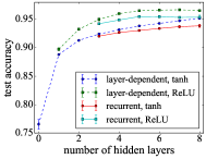
Figure 2: Test accuracy of trained fully connected DNNs applied on the MNIST dataset. Images have been downsampled by a factor of $2$ to reduce training time, and each hidden layer has $128$ nodes. Each data point is averaged over $5$ random initializations. The accuracies of recurrent architectures, with weight Fsharing between hidden layers, are comparable to those of layer-dependent architectures.

Boolean functions computed at large depth.––We consider the typical Boolean functions computed in random-layered machines by examining $P^{L}(\bm{f})$ in the large depth limit $L\rightarrow\infty$ for specific gates in the following examples.

In DNNs using the ReLU activation function $\alpha^{l}(x)=\max(x,0)$, in the hidden layers (the sign activation function is always used in the output layer), which is commonly used in applications, all covariance matrix elements $\left[\bm{c}^{L}\right]_{\gamma\gamma^{\prime}}$ in the Eq. (7) converge to the same value in the limit $L\to\infty$, implying that all components of the preactivation field vector $\bm{h}$ are also the same and hence the components of $\bm{f}$ are identical. Therefore, random deep ReLU networks compute only constant Boolean functions in the infinite depth limit, echoing recent findings of a bias toward simple functions in random DNNs constructed from ReLUs Mozeika2020sup , which arguably plays a role in their generalization ability Valle-Perez2018 ; Palma2019 .

In DNNs using sign activation function also in hidden layers, i.e., Eq. (1) enforces the rule $S_{i}^{l}=\mathrm{sgn}(\sum_{j}W_{ij}^{l}S_{j}^{l-1}/\sqrt{N})$, those cross-pattern overlaps $q_{\gamma\gamma^{\prime}}^{l}=(1/N)\sum_{i}\overline{\langle S_{i,\gamma}^{l}S_{i,\gamma^{\prime}}^{l}\rangle}$ satisfying $|q_{\gamma\gamma^{\prime}}^{l}|<1$ monotonically decrease with an increasing number of layers and vanish as $l\rightarrow\infty$, such “chaotic” nature of dynamics also holds in random DNNs with other sigmoidal activation functions such as the error and hyperbolic tangent functions Poole2016 ; Yang2019 . The consequences of this behavior is that for the input vector $\vec{S}^{I}=\vec{s}$, $P^{L}(\bm{f})$ is uniform on the set of all odd functions Mozeika2020sup , i.e., functions satisfying $f(-\vec{s})=-f(\vec{s})$. Furthermore, for $\vec{S}^{I}=(\vec{s},1)$, $P^{L}(\bm{f})$ is uniform on the set of all Boolean functions Mozeika2020sup .

For Boolean circuits, there are also scenarios where the distribution $P^{L}(\bm{f})$ has a single Boolean function in its support or it is uniform over some set of functions Savicky1990 ; Brodsky2005 ; Mozeika2010 . The latter depends on the gates $\alpha$ used in Eq. (1) and input vector $\vec{S}^{I}$. For example, in the AND gate with $\alpha(S_{1},S_{2})=\mathrm{sgn}(S_{1}+S_{2}+1)$ or the OR gate with $\alpha(S_{1},S_{2})=\mathrm{sgn}(S_{1}+S_{2}-1)$ Mozeika2020sup , their output is biased, respectively, toward $+1$ or $-1$ Savicky1990 ; Mozeika2010 ; Mozeika2020sup . The consequence of the latter is that the distribution $P^{L}(\bm{f})$ has only a single Boolean function in its support Mozeika2010 ; Mozeika2020sup . On the other hand, when the majority gate $\alpha(S_{1},...,S_{k})=\mathrm{sgn}(\sum_{j=1}^{k}S_{j})$, which is balanced $\sum_{S_{1},...,S_{k}}\alpha(S_{1},...,S_{k})=0$ and nonlinear , is used with the input vector $\vec{S}^{I}=(\vec{s},-\vec{s},1,-1)$, then the distribution $P^{L}(\bm{f})$ is uniform over all Boolean functions Mozeika2010 , which is consistent with the result of Savicky1990 .

Entropy of Boolean functions.––Having considered the distribution of Boolean functions for a few different examples, we observed that random-layered machines either reduce to a single Boolean function or compute all (or a subset of) functions with a uniform probability on the layer $L$, as $L\rightarrow\infty$. We note that for the Shannon entropy over Boolean functions $\mathcal{H}^{L}=-\sum_{\bm{f}}P^{L}(\bm{f})\log P^{L}(\bm{f})$, these two scenarios saturate its lower and upper bounds, respectively, given by $0$ and $2^{n}\log 2$. Thus, the entropy $\mathcal{H}^{L}$ can be seen, at least intuitively, as a measure of function space complexity.

In Fig. 3, we study the entropy $\mathcal{H}^{L}$, computed using Eqs. (7) and (Space of Functions Computed by Deep-Layered Machines), as a function of the depth $L$ in random-layered machines constructed from different activation functions or gates and computing different inputs. The initial increase in entropy after layer $L=0$, seen in Fig. 3(a), (b), can be explained by the properties of gates used and the initial set of (simple) Boolean functions at layer $L=0$; functions from the layer $L=0$ are “copied” onto layer $L=1$, while new functions are also created, as illustrated in Fig. 3(c), (d). Note that the minimal depth in ReLU networks to produce a Boolean function is $L=2$. The dependence of entropy $\mathcal{H}^{L}$ on $L$ after the initial increase depends on the specific gate functions used. For the ReLU activation function in DNNs and the AND gate in Boolean circuits, the entropies $\mathcal{H}^{L}$ monotonically decrease with $L$, suggesting that sizes of sets of typical Boolean functions computed are decreasing with increasing numbers of layers $L$. Random initialization of layered machines with such gates/activation functions serves as a biasing prior toward a more restricted set of functions Valle-Perez2018 ; Palma2019 . On the other hand, for balanced gates, with appropriate initial conditions, e.g., sign in DNNs and majority vote in Boolean circuits, the entropy $\mathcal{H}^{L}$ is monotonically increasing with the depth $L$, indicating that the sizes of sets of the typical Boolean functions computed are increasing.

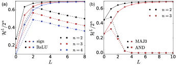
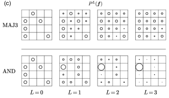
Figure 3: Normalized entropy and distribution of functions of deep-layered machines. (a) Normalized entropy $\mathcal{H}^{L}/2^{n}$ of Boolean functions computed by DNNs with sign or ReLU activation in the hidden layers as a function of the network depth $L$; the initial condition is set as $\vec{S}^{I}=(\vec{s},1)$. (b) $\mathcal{H}^{L}/2^{n}$ vs $L$ for Boolean circuits constructed by MAJ3 or the AND gate with initial condition $\vec{S}^{I}=(\vec{s},-\vec{s},1,-1)$. (c) The distribution of Boolean functions $P^{L}(\bm{f})$ computed by Boolean circuits with two inputs $n=2$ (the number of all possible functions is $16$) is represented by the sizes of circles on a $4\times 4$ grid. Upper panel: MAJ3-gate-based circuits, in which more functions are created at larger depth $L$ and $P^{L}(\bm{f})$ converges to a uniform distribution. Lower panel: AND-gate-based circuits, in which new functions are created from $L=0$ to $L=1$, while $P^{L}(\bm{f})$ converges to a distribution with supports in a single Boolean function as network depth increases.

In summary, we present an analytical framework to examine Boolean functions represented by random deep-layered machines, by considering all possible inputs simultaneously and applying the generating functional analysis to compute various relevant macroscopic quantities. We derived the probability of Boolean functions computed on the output nodes. Surprisingly, we discover that the typical sets of Boolean functions computed by the layer-dependent and recurrent architectures are identical. It points to the possibility of computing complex functions with a reduced number of parameters by weight or connection sharing, as showcased in an image classification experiment. We also study the Boolean functions computed by specific random-layered machines. Biased activation functions (e.g., ReLU) or biased Boolean gates (e.g., AND/OR) can lead to more restricted typical sets of Boolean functions found at deeper layers, which may explain their generalization ability. On the other hand, balanced activation functions (e.g., sign) or Boolean gates (e.g., majority) complemented with appropriate initial conditions, lead to a uniform distribution on all Boolean functions at the infinite depth limit. It will be interesting to investigate the functions realized by different DNN architectures with structured data and by different learning algorithms Saad1998 ; Goldt2020 ; Pastore2020 ; Rotondo2020 ; Zdeborova2020 .

We also showed the monotonic behavior of the entropy of Boolean functions as a function of depth, which is of interest in the field of computer science. We envisage that the insights gained and the methods developed will facilitate further study of deep-layered machines.

- [1] Yann LeCun, Yoshua Bengio, and Geoffrey Hinton. Deep learning. Nature, 521(7553):436–444, 2015.
- [2] Ryan O’Donnell. Analysis of Boolean Functions. Cambridge University Press, New York, 2014.
- [3] Kurt Hornik, Maxwell Stinchcombe, and Halbert White. Multilayer feedforward networks are universal approximators. Neural Networks, 2(5):359 – 366, 1989.
- [4] Ben Poole, Subhaneil Lahiri, Maithreyi Raghu, Jascha Sohl-Dickstein, and Surya Ganguli. Exponential expressivity in deep neural networks through transient chaos. In D. D. Lee, M. Sugiyama, U. V. Luxburg, I. Guyon, and R. Garnett, editors, Advances in Neural Information Processing Systems 29, pages 3360–3368. Curran Associates, Inc., New York, 2016.
- [5] N. Nisan and S. Schocken. The Elements of Computing Systems: Building a Modern Computer from First Principles. MIT Press, 2008.
- [6] Andreas Engel and Christian Van den Broeck. Statistical Mechanics of Learning. Cambridge University Press, New York, 2001.
- [7] David Saad, editor. On-Line Learning in Neural Networks. Cambridge University Press, New York, 1998.
- [8] Elena Agliari, Adriano Barra, Andrea Galluzzi, Francesco Guerra, and Francesco Moauro. Multitasking associative networks. Phys. Rev. Lett., 109:268101, 2012.
- [9] Haiping Huang and Taro Toyoizumi. Advanced mean-field theory of the restricted boltzmann machine. Phys. Rev. E, 91:050101, 2015.
- [10] Marylou Gabrié, Eric W Tramel, and Florent Krzakala. Training restricted boltzmann machine via the thouless-anderson-palmer free energy. In C. Cortes, N. D. Lawrence, D. D. Lee, M. Sugiyama, and R. Garnett, editors, Advances in Neural Information Processing Systems 28, pages 640–648. Curran Associates, Inc., 2015.
- [11] Marc Mézard. Mean-field message-passing equations in the hopfield model and its generalizations. Phys. Rev. E, 95:022117, 2017.
- [12] Adriano Barra, Giuseppe Genovese, Peter Sollich, and Daniele Tantari. Phase diagram of restricted boltzmann machines and generalized hopfield networks with arbitrary priors. Phys. Rev. E, 97:022310, 2018.
- [13] J J Hopfield. Neural networks and physical systems with emergent collective computational abilities. Proceedings of the National Academy of Sciences, 79(8):2554–2558, 1982.
- [14] J.A. Hertz, A.S. Krogh, and R.G. Palmer. Introduction To The Theory Of Neural Computation. Addison-Wesley, 1991.
- [15] J. J. Hopfield. Learning algorithms and probability distributions in feed-forward and feed-back networks. Proceedings of the National Academy of Sciences, 84(23):8429–8433, 1987.
- [16] Petr Savický. Random boolean formulas representing any boolean function with asymptotically equal probability. Discrete Mathematics, 83(1):95 – 103, 1990.
- [17] Alex Brodsky and Nicholas Pippenger. The boolean functions computed by random boolean formulas or how to grow the right function. Random Structures & Algorithms, 27(4):490–519, 2005.
- [18] Jaehoon Lee, Jascha Sohl-dickstein, Jeffrey Pennington, Roman Novak, Sam Schoenholz, and Yasaman Bahri. Deep neural networks as gaussian processes. In Proceedings of the 6th International Conference on Learning Representations, 2018.
- [19] Bo Li and David Saad. Exploring the function space of deep-learning machines. Phys. Rev. Lett., 120:248301, 2018.
- [20] Bo Li and David Saad. Large deviation analysis of function sensitivity in random deep neural networks. Journal of Physics A: Mathematical and Theoretical, 53(10):104002, 2020.
- [21] Alexander Mozeika, David Saad, and Jack Raymond. Computing with noise: Phase transitions in boolean formulas. Phys. Rev. Lett., 103:248701, 2009.
- [22] See Supplemental Material for details, which includes Refs. [41, 42, 43].
- [23] Marc Mézard, Giorgio Parisi, and Miguel Virasoro. Spin glass theory and beyond: An Introduction to the Replica Method and Its Applications, volume 9. World Scientific Publishing Co Inc, 1987.
- [24] Greg Yang and Hadi Salman. A fine-grained spectral perspective on neural networks. arXiv:1907.10599, 2019.
- [25] A.C.C. Coolen. Chapter 15 statistical mechanics of recurrent neural networks ii - dynamics. In F. Moss and S. Gielen, editors, Neuro-Informatics and Neural Modelling, volume 4 of Handbook of Biological Physics, pages 619 – 684. North-Holland, 2001.
- [26] Taro Toyoizumi and Haiping Huang. Structure of attractors in randomly connected networks. Phys. Rev. E, 91:032802, 2015.
- [27] A. Crisanti and H. Sompolinsky. Path integral approach to random neural networks. Phys. Rev. E, 98:062120, 2018.
- [28] Viewing the layers as time steps, the functions can be seen as molecules of gas undergoing -body collisions.
- [29] B. Cessac. Increase in complexity in random neural networks. J. Phys. I France, 5(3):409–432, 1995.
- [30] J P L Hatchett, B Wemmenhove, I Pérez Castillo, T Nikoletopoulos, N S Skantzos, and A C C Coolen. Parallel dynamics of disordered ising spin systems on finitely connected random graphs. Journal of Physics A: Mathematical and General, 37(24):6201–6220, 2004.
- [31] Y. Cheng, D. Wang, P. Zhou, and T. Zhang. Model compression and acceleration for deep neural networks: The principles, progress, and challenges. IEEE Signal Processing Magazine, 35(1):126–136, 2018.
- [32] Yann LeCun, Corinna Cortes, and Christopher J. Burges. The MNIST Database of Handwritten Digits (1998), http://yann.lecun.com/exdb/mnist/.
- [33] Guillermo Valle-Perez, Chico Q. Camargo, and Ard A. Louis. Deep learning generalizes because the parameter-function map is biased towards simple functions. In Proceedings of the 7th International Conference on Learning Representations. 2019.
- [34] Giacomo De Palma, Bobak Kiani, and Seth Lloyd. Random deep neural networks are biased towards simple functions. In H. Wallach, H. Larochelle, A. Beygelzimer, F. d'Alché-Buc, E. Fox, and R. Garnett, editors, Advances in Neural Information Processing Systems 32, pages 1962–1974. Curran Associates, Inc., 2019.
- [35] Alexander Mozeika, David Saad, and Jack Raymond. Noisy random boolean formulae: A statistical physics perspective. Phys. Rev. E, 82:041112, 2010.
- [36] Since are binary variables in the context of Boolean circuits, linearity is defined in the finite field [16, 17].
- [37] Sebastian Goldt, Marc Mézard, Florent Krzakala, and Lenka Zdeborová. Modelling the influence of data structure on learning in neural networks: the hidden manifold model. arXiv:1909.11500, 2019.
- [38] Pietro Rotondo, Mauro Pastore, and Marco Gherardi. Beyond the storage capacity: Data-driven satisfiability transition. Phys. Rev. Lett., 125:120601, Sep 2020.
- [39] Mauro Pastore, Pietro Rotondo, Vittorio Erba, and Marco Gherardi. Statistical learning theory of structured data. Phys. Rev. E, 102:032119, Sep 2020.
- [40] Lenka Zdeborová. Understanding deep learning is also a job for physicists. Nature Physics, 16(6):602–604, 2020.
- [41] B Derrida, E Gardner, and A Zippelius. An exactly solvable asymmetric neural network model. Europhysics Letters (EPL), 4(2):167–173, 1987.
- [42] R. Kree and A. Zippelius. Continuous-time dynamics of asymmetrically diluted neural networks. Phys. Rev. A, 36:4421–4427, 1987.
- [43] Diederik P. Kingma and Jimmy Ba. Adam: A method for stochastic optimization. In Proceedings of the 3rd International Conference on Learning Representations. 2015.