Can axion clumps be formed in a pre-inflationary scenario?

Abstract

The QCD axion and an axion-like particle (ALP) are compelling candidates of dark matter. For the QCD axion, it is known that when the Peccei-Quinn (PQ) symmetry is spontaneously broken after inflation, the large initial fluctuation can lead to axion clump formation. On the other hand, when the symmetry is already broken during inflation, it has been believed that the axion clump formation does not occur due to the small amplitude of the initial axion fluctuation. We revisit this prevailing understanding, considering both the QCD axion and an ALP. We find that for the QCD axion, the clump formation does not occur even if we consider an extremely fine-tuned initial condition. Meanwhile, it turns out that for an ALP which allows a more general potential form, the clump formation can take place through the tachyonic instability or/and the resonance instability, considering a multiple cosine potential.

1 Introduction

Dark matter (DM) is one of the puzzles in cosmology and particle physics to be solved. Since this essence cannot be explained within the standard model of particle physics, a new physics beyond the standard model is required to approach DM. Up until now, a variety of DM candidates have been considered. Axion or more generally axion-like particle (ALP) is one of the best-motivated candidates of DM.

Axion is a hypothetical particle introduced to solve the strong CP problem in quantum chromodynamics (QCD). The strong CP problem is related to a term that breaks CP symmetry in the QCD Lagrangian. The CP violation is characterized by a constant parameter $\theta_{{\rm QCD}}$, which can be examined by measuring the neutron electric dipole moment. From the current measurement, $\theta_{{\rm QCD}}$ is bounded as $|\theta_{{\rm QCD}}|\lesssim 10^{-10}$ [1]. Such an unnaturally small CP violation cannot be explained within the standard model. In the Peccei-Quinn (PQ) mechanism, which was proposed to solve this problem [2, 3], the $\theta_{\rm QCD}$ term goes to zero dynamically. The additionally introduced field for a realization of this mechanism is called QCD axion [4, 5]. Soon after the original QCD axion model was ruled out because of the inconsistency with the electroweak physics, the invisible axion models were proposed [6, 7, 8, 9]. In Refs. [10, 11, 12], it was pointed out that the invisible axion can play the role of DM, when it oscillates coherently around the potential minimum. For a review, see e.g., Refs. [13, 14, 15].

Regarding cosmological aspect of the QCD axion, the key indicator is whether the PQ symmetry was already broken during inflation or has been broken after inflation. The former is the case when the PQ symmetry breaking scale, $f$, is comparable to or larger than the energy scale of inflation, characterized by the Gibbons-Hawking temperature, $T_{\rm GH}=H_{I}/2\pi$, with $H_{I}$ being the Hubble parameter during inflation, while the latter is the case when $f$ is smaller than $T_{\rm GH}$. The former is called pre-inflationary scenario and the latter is called post-inflationary scenario. When the PQ symmetry is already broken during inflation, satisfying $f>H_{I}/2\pi$, the inflation makes the axion field value almost homogeneous at least in our observable patch of the Universe. Then, the field fluctuation, corresponding to isocurvature fluctuation, is typically small, being consistent with CMB observations. On the other hand, when the PQ symmetry is restored during inflation, i.e. $f<H_{I}/2\pi$, the spontaneous symmetry breaking occurs after inflation, which results in a lot of causally-disconnected patches that have different initial field values. It leads to the formation of topological defects [16]. After the decay of topological defects, the field fluctuation can be $\mathcal{O}(1)$ on sub-horizon scales.

In the post-inflationary scenario, Kolb and Tkachev [17, 18, 19] pointed out that when the axion potential switches on in the QCD epoch and the the axion commences the coherent oscillation, the fluctuation in the initial misalignment is transformed into the fluctuation in the energy density of the axion. Subsequently, the non-linear dynamics driven by the attractive self-interaction of the axion leads to formation of overdense axion clumps, called axiton [18] or axion miniclusters [20]. The formed axion overdense clumps undergo the non-linear gravitational collapse, as was addressed by conducting the $N$-body simulation in Ref. [21]. More recently, in Ref. [22], the formation and clustering of axion minihalos were studied based on $N$-body simulation to date. In Ref. [23], it was argued that the tidal disruption may have a significant impact on the succeeding evolution. A semi-analytic computation of the mass function for axion miniclusters can be found in Ref. [24]. A review on axion miniclusters can be found e.g., in Ref. [25].

The formation of axion clumps can leave an interesting phenomenological consequence, opening a window for axion search. In Refs. [17, 26], it was conjectured that axion stars, which are gravitationally bound and stable, may appear in the center of axion miniclusters through further contraction. More recent studies on axion stars include [27, 28, 29, 30]. Axion clumps can cause gravitational lensing effect, which may be detectable through femtolensing and picolensing measurements [31] and microlensing measurements [32, 33, 34].

On the other hand, the possibility of the clump formation has not been well investigated, when the PQ symmetry was already broken during inflation, i.e., in pre-inflationary scenario. This is presumably because the initial fluctuation of the axion has been considered to be too small for the formation of axiton or axion miniclusters. Meanwhile, especially in the context of reheating, it is known that a similar overdense clump, called oscillons [35, 36, 37, 38, 39, 40, 41], can be formed for a wide class of scalar field models with an attractive self-interaction, even if we start with an almost homogeneous initial condition. As we increase the misalignment angle, being away from the potential minimum, the quartic term, which yields an attractive force, becomes more important. In an extreme case where the axion was located around the hilltop of the potential just after it acquires the potential, the fluctuation of the axion is expected to be enhanced by the tachyonic instability. Furthermore, since the tachyonic mass of the axion, $-m^{2}$, increases with time through the QCD instanton effect, one may expect that the tachyonic instability can be more efficient in the QCD epoch. A possible impact of the tachyonic instability on the axion isocurvature was studied in Ref. [42] by taking the large scale limit, where the $\delta N$ formalism [43, 44, 45] can be adopted. In this paper, we study the possibility of QCD axion clump formation in the pre-inflationary scenario, while accepting a fine-tuned initial condition. In Ref. [46], a dynamical mechanism which places the axion at the hilltop was proposed. For our purpose, we should also take into account the spatial gradient of the axion configuration, in contrast to the situation addressed in Ref. [42].

The compelling aspect of the QCD axion which enables to play the role of dark matter motivates us to consider a more general framework of axion like particle (ALP). Furthermore, ALPs are ubiquitously predicted in low energy effective field theories of string theory [47] (see also Refs. [48, 49]). ALPs have various common aspects with the QCD axion e.g., behaving as non-relativistic matter during the coherent oscillation and an anomalous coupling with photons. Meanwhile, unlike the QCD axion, the shape and height of ALP potential are not necessarily determined by the QCD dynamics. This leaves a wider parameter space for ALPs to become dark matter. Taking the uncertainty of the ALP potential granted, in this paper, we also address the possibility of ALP clump formation for a generalized form of the potential that includes several cosine terms. We maintain the quadratic form around the potential minimum so that the ALP can become dark matter at a later time. Such a multiple cosine potential has been discussed for axion inflation models [50, 51].

The ALP potential with two cosine terms can have a shallower region than the quadratic form. It has been widely known that the tachyonic instability and/or the resonance instability can be significant for such a potential (see e.g., Refs. [52, 53, 54]). When the potential is shallow enough, subsequently, overdense clumps, called oscillon, can be formed. It was pointed out that during the oscillon formation process, the gravitational waves can be copiously produced by considering axion inflation [55, 56, 57, 58, 59] and axion dark matter [53, 60]. In Refs. [61, 62], it was shown that these instabilities of ALPs also can provide a primordial origin of intergalactic magnetic fields.

This paper is organized as follows. In Sec. 2 we briefly summarize the property of QCD axion and ALP. In Sec. 3, we investigate the clump formation of the QCD axion when the PQ symmetry was already broken during inflation. In Sec. 4, we analyze clump formation for ALPs, clarifying several different formation processes. Finally, in Sec. 5, we summarize our results.

2 Basic property of QCD axion and ALPs

In this section, first we describe the setup of the problem with a brief review. Focusing on the axion which commences its oscillation during radiation domination, we ignore the contribution of the axion to the geometry of the Universe.

2.1 Axion potential and relic abundance

At the QCD phase transition, the QCD axion acquires the potential through the QCD instanton effect. The height of the potential is determined by the QCD scale, $\chi_{{\rm QCD}}$, which is called the QCD topological susceptibility. Here we adopt the results of the lattice QCD simulation in Ref. [63], where $\chi_{{\rm QCD}}$ is approximately given by

$$\chi_{{\rm QCD}}(T)=\frac{\chi_{0}}{1+(T/T_{c})^{b}},$$ (2.1)

with $\chi_{0}=(7.6\times 10^{-2}\ {\rm GeV})^{4}$, $T_{c}=0.16$ GeV and $b=8.2$. Here, $T$ should be understood as the temperature of the relativistic species, which dominate the Universe. When the dilute instanton gas approximation (DIGA) holds, the potential of the QCD axion, $\phi$, is given by

$$V(\phi)=\chi_{{\rm QCD}}(T)(1-\cos(\phi/f)).$$ (2.2)

The potential form slightly differs from the one computed from the low energy effective Lagrangian in Ref. [64]. A detailed study about the potential form of the QCD axion and the coupling with the standard model sector can be found, e.g., in Refs. [65, 66, 67, 68].

For $T>T_{\rm c}$, as the temperature decreases, the mass of axion, given by

$$m(T)=\sqrt{\chi_{\rm QCD}(T)}/f\,,$$ (2.3)

increases as $m(T)\propto T^{-b/2}$. Meanwhile, for $T<T_{\rm c}$, $m(T)$ approaches to a constant value, given by

$$m_{0}\simeq 6\,\mu{\rm eV}\left(\frac{10^{12}\,{\rm GeV}}{f}\right).$$ (2.4)

The axion commences oscillation at $T_{\ast}$ satisfying $3H(T_{\ast})=m(T_{\ast})\equiv m_{\ast}$ with $H(T)$ the Hubble parameter, and for $T_{\ast}>T_{c}$, $T_{\ast}$ is given by

$$T_{\ast}\simeq 1.0\,{\rm GeV}\left(\frac{10^{12}\,{\rm GeV}}{f}\right)^{0.16}.$$ (2.5)

Then, one can obtain the final QCD axion abundance as (see also Refs. [69, 66, 70])

$$\Omega_{a}h^{2}=0.10\kappa\left(\frac{f\tilde{\phi}_{i}}{10^{12}\,{\rm GeV}}\right)^{1.16}F(\tilde{\phi}_{i}),$$ (2.6)

where $\kappa$ is ${\cal O}(1)$ numerical factor characterizing nonadiabaticity and $F(\tilde{\phi}_{i})$ is anharmonic correction factor which is a function of the initial value of $\tilde{\phi}=\phi/f$, which becomes significant when the initial value is placed near the top of the cosine potential. The anharmonic correction $F(\tilde{\phi}_{i})$ was computed, e.g., in Refs. [69, 71, 72]. Note that the QCD axion with the decay constant being $f\sim 10^{12}$ GeV and the initial value being $\tilde{\phi}_{i}\sim 1$ saturates the DM relic abundance in the Universe, corresponding to the upper bound of the so called "classical axion window" [73], given by

$$4\times 10^{8}{\rm GeV}<f<10^{12}{\rm GeV},$$ (2.7)

where the lower bound comes from neutrino burst duration of SN1987A [74]. Note that this upper bound includes a large ambiguity, because $\Omega_{a}h^{2}$ highly depends on the cosmological scenario.

2.2 Potential of ALPs

In the case of ALPs, the potential can take a more general form, since it is not necessarily determined by the QCD physics. It is known that ALPs predicted in string theory generically acquire multiple cosine terms through the non-perturbative corrections as

$$V(\phi)=-\sum_{i=1}^{n}\Lambda_{i}^{4}\cos\left(\frac{\phi}{f_{i}}+\Theta_{i}\right)+{\rm const.},$$ (2.8)

where $\Lambda_{i}$, $f_{i}$ and $\Theta_{i}$ are model parameters. An inflation model with multiple cosine terms was studied e.g., in alignment models [75, 76] and multi-natural inflation model [50].

Here and in what follows, generalizing a single cosine potential, we consider two cosine terms whose amplitudes are given by $\Lambda_{1}^{4}=\Lambda_{2}^{4}/(4+\epsilon)=m^{2}(T)f^{2}$ and the periods are given by $f_{1}=f_{2}/2=f$ as

$$V(\phi)=\frac{m^{2}(T)f^{2}}{2(1+\epsilon/8)}\left[5+\epsilon-\cos\left(\frac{\phi}{f}\right)-(4+\epsilon)\cos\left(\frac{\phi}{2f}\right)\right]$$ (2.9)

with a constant parameter $\epsilon$ and $\Theta_{1}=\Theta_{2}=0$. With this choice, the potential satisfies

$$V(0)=0\,,\qquad V(\phi)\sim\frac{m^{2}(T)}{2}\phi^{2}\quad(|\phi|\to 0)\,,$$ (2.10)

where the second condition ensures that the ALP can behave as dark matter at a later time. When we set $\epsilon=-4$, the potential (2.9) corresponds to the single cosine case given by Eq. (2.2). Figure 1 shows the potential shape of Eq. (2.9) for several values of $\epsilon$. It should be emphasized that, in the limit $\epsilon\to 0$, the quadratic term in the power series of cosine terms vanishes around the maximum of the potential and the quartic term becomes important. In that case, the potential hill becomes flatter as one can see in Fig. 1.

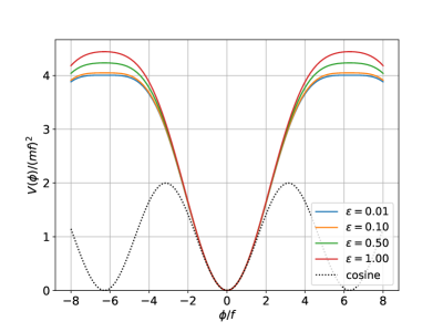
Figure 1: This plot shows the potential (2.9) for $\epsilon=0.01,0.1,0.5,1.0$. The vertical axis denotes $V/(m(T)f)^{2}$. The black dotted line shows the cosine potential, given in Eq. (2.2), which corresponds to $\epsilon=-4$.

Here we consider the temperature dependence of the ALP mass since interactions between the ALP and hidden sector gauge fields can in general introduce such a temperature dependence. Likewise the QCD axion, we parametrize the temperature dependence of the ALP mass as

$$m^{2}(T)=\frac{m^{2}_{0}}{1+(T/T_{c})^{b}},$$ (2.11)

where $m_{0}$ denotes the ALP mass evaluated at $T=0$ and $T_{c}$ and $b$ are parameters depending on the hidden sector physics. In particular, $T_{c}$ can be different from the QCD confinement scale.

2.3 Field evolution

In the flat-FLRW Universe, the evolution equation of the axion is given by

$$\frac{\partial^{2}}{\partial\tilde{t}^{2}}\tilde{\phi}+3\frac{H}{m_{\ast}}\frac{\partial}{\partial\tilde{t}}\tilde{\phi}-\frac{\partial^{2}_{\tilde{\hbox{\boldmath{\scriptsize$x$}}}}}{a^{2}}\tilde{\phi}+\tilde{V}_{\tilde{\phi}}=0,$$ (2.12)

where $\tilde{t}\equiv m_{\ast}t$, $\tilde{\hbox{\boldmath{$x$}}}\equiv m_{\ast}\hbox{\boldmath{$x$}}$, $\tilde{V}=V/(m_{\ast}f)^{2}$, $\tilde{V}_{\tilde{\phi}}=d\tilde{V}/d\tilde{\phi}$ and $a$ is the scale factor. In the radiation dominated Universe with $a\propto t^{1/2}$, the Hubble parameter is given by $H/m_{*}=1/(2\tilde{t})\propto T^{2}$.

For the homogeneous mode of $\tilde{\phi}$, the evolution equation is given by

$$\frac{d^{2}}{d\tilde{t}^{2}}\tilde{\phi}+3\frac{H}{m_{\ast}}\frac{d}{d\tilde{t}}\tilde{\phi}+\tilde{V}_{\tilde{\phi}}=0.$$ (2.13)

When the axion mass is much smaller than the Hubble parameter, the axion field remains a constant value. On the other hand, when the temperature becomes lower than $T_{\ast}$ and the mass of the axion becomes larger than the Hubble parameter, the axion starts to oscillate. Perturbing Eq.(2.12), the evolution equation of the linear perturbation $\delta\tilde{\phi}\equiv\delta\phi/f$ reads

$$\frac{d^{2}}{d\tilde{t}^{2}}\delta\tilde{\phi}_{k}+3\frac{H}{m_{\ast}}\frac{d}{d\tilde{t}}\delta\tilde{\phi}_{k}+\left(\left(\frac{k}{am_{\ast}}\right)^{2}+\tilde{V}_{\tilde{\phi}\tilde{\phi}}\right)\delta\tilde{\phi}_{k}=0,$$ (2.14)

where $\delta\tilde{\phi}_{k}$ denotes the Fourier mode of $\delta\tilde{\phi}$, $\tilde{V}_{\tilde{\phi}\tilde{\phi}}\equiv d^{2}\tilde{V}/d\tilde{\phi}^{2}$, and we neglect the metric perturbation. From the next section, we analyze clump formation, considering the QCD axion and ALPs in turn.

3 Clump formation: QCD axion

In this section, we discuss the possibility of the clump formation for the QCD axion which commences the oscillation at the QCD epoch, taking into account the thermal correction to the axion mass [63].

3.1 Linear calculation

When the misalignment axion is initially located around the top of the potential, it rolls down the region where the potential curvature, given by $\tilde{V}_{\tilde{\phi}\tilde{\phi}}=(m(T)/m_{\ast})^{2}\cos\tilde{\phi}$, becomes negative before the onset of the oscillation. Then, the the coefficient of $\delta\tilde{\phi}_{k}$ in Eq.(2.14) can be negative for the modes that satisfy

$$\frac{k}{am_{\ast}}<\frac{m(T)}{m_{\ast}}.$$ (3.1)

Using Eqs.(2.13) and (2.14), the temperature dependence of the axion mass is given by

$$\left(\frac{m(T)}{m_{\ast}}\right)^{2}=\left(\frac{f}{10^{12}{\rm GeV}}\right)^{-2}\left(\frac{m_{\ast}}{10^{-9}{\rm eV}}\right)^{-2}\frac{(7.6\times 10^{-2})^{4}}{1+(T/T_{c})^{b}}.$$ (3.2)

The Fourier mode of the fluctuation that satisfy Eq. (3.1) grows exponentially due to tachyonic instability. As discussed in Ref. [54], the parametric resonance instability hardly takes place for the cosine potential. Furthermore, the time variation of $m$ makes the resonance even more difficult, since the periodicity of the oscillation changes in time. Therefore, the efficiency of the tachyonic instability is an important factor for the clump formation. As a situation where we expect the maximum enhancement through the tachyonic instability, we consider the case where the axion was initially located around the hilltop of the cosine potential, i.e., $\tilde{\phi}_{i}\simeq\pi$. An interesting example where tachyonic instability leads to formation of clumpy structure is Q-ball formation, studied e.g., in Refs. [77, 78, 79] (see also Ref. [80]).

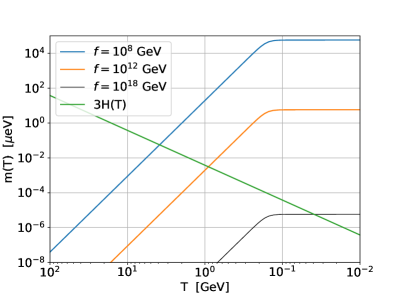
Figure 2: This plot shows the $T$ dependence of the Hubble parameter $H$ and the axion mass $m$.

For a given decay constant $f$, the temperature $T_{\ast}$ with $3H(T_{\ast})=m(T_{\ast})$ is uniquely determined. Figure 2 shows the evolution of the Hubble parameter $H$ and the axion mass $m$ for $f=10^{8}$ GeV (blue) and $f=10^{12}$ GeV (orange). Notice that as long as the phenomenological constraint on $f$, given in Eq. (2.7), is satisfied, the QCD axion commences the oscillation in the QCD epoch, taking $T_{\ast}\sim{\cal O}({\rm GeV})$. For a comparison, we also show the axion mass for $f=10^{18}$ GeV, for which, the axion mass has already reached $m_{0}$ at $T=T_{\ast}$.

The Fourier modes in the range (3.1) exponentially grow as $\delta\tilde{\phi}_{k}\propto e^{\mu_{k}m_{\ast}t}$ with the dimensionless growth rate $\mu_{k}$, which is roughly estimated as

$$\mu_{k}\simeq\sqrt{\left(\frac{m(T)}{m_{\ast}}\right)^{2}-\left(\frac{k}{am_{\ast}}\right)^{2}}$$ (3.3)

for $\tilde{\phi}\sim\pi$. For a smaller $k$, the growth rate becomes larger. In the limit $k/a\ll m(T)$, $\mu_{k}$ is given by $\mu_{k}\simeq m(T)/m_{\ast}$, implying that the growth rate $\mu_{k}$ becomes larger and larger as $m(T)$ increases.

The clump formation becomes more probable as $\tilde{\phi}_{i}$ is closer to $\pi$ and as the initial amplitude of the fluctuation $\delta\phi_{i}$ is larger. Meanwhile, when the amplitude of the initial fluctuation $\delta\phi_{i}$ is larger than the initial deviation from the top of the potential $|\tilde{\phi}_{i}-\pi|$, one spatial patch rolls down towards $\tilde{\phi}=0$ and another towards $\tilde{\phi}=2\pi$, leading to formation of domain walls. Therefore, an initial condition where the clump formation is the most probable but the domain wall formation can be marginally avoided, we employ

$$\tilde{\phi}_{i}=\pi\times(1-10^{-8})\,,\qquad\delta\tilde{\phi}_{i}=\pi\times 10^{-8}\,.$$ (3.4)

The initial velocity of $\tilde{\phi}$ is determined by imposing the slow-roll condition as

$$\frac{d\tilde{\phi}}{d\tilde{t}}\bigg{|}_{\tilde{t}=\tilde{t}_{i}}=-\frac{\tilde{V}_{\tilde{\phi}}(\tilde{\phi}_{i})}{3H_{i}/m_{\ast}}=-\left(\frac{T_{\ast}}{T_{i}}\right)^{2}\frac{7.6^{4}\times 10^{-8}}{(f/10^{12}{\rm GeV})^{2}(m_{\ast}/10^{-9}{\rm eV})^{2}(1+(T_{i}/T_{c})^{b})}\sin\tilde{\phi}_{i}.$$ (3.5)

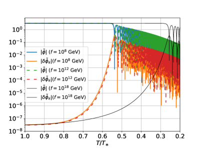
Figure 3: This panel shows the time evolution of the background homogeneous mode and the inhomogeneous mode with $k/(a_{\ast}m_{\ast})=0.1$ for $f=10^{8}$ GeV and $f=10^{12}$ GeV. The horizontal axis is the temperature normalized by $T_{\ast}$. For a comparison, we also show the time evolution for $f=10^{18}$ GeV, for which the axion mass remains time independent during the tachyonic instability.

Figure 3 shows the time evolution of $\tilde{\phi}$ and $\delta\tilde{\phi}_{k}$. Here, the temperature of radiation is used as a corresponding time variable. The wavenumber $k$ is set to $k/(a_{\ast}m_{\ast})=0.1$, which satisfies the condition for the tachyonic instability, (3.1). The temperature in the horizontal axis is normalized by $T_{\ast}$ to compare the evolution for different values of $f$, for which the axion commences the oscillation at different moments. For $f=10^{8}$ GeV and $f=10^{12}$ GeV, the period of the oscillation becomes shorter and shorter, since the axion mass still keeps on changing for a while after $T_{\ast}$. In both cases, the axion mass keeps on increasing as $m(T)\propto T^{-b/2}$ during the growth due to the tachyonic instability, the time evolution remains almost the same. The tachyonic instability terminates at the commencement of the oscillation.

For a comparison, in Fig. 3, we have also plotted the evolution of $\tilde{\phi}$ and $\delta\tilde{\phi}_{k}$ for $f=10^{18}$ GeV, while it does not satisfy Eq. (2.7). In this case, as shown in Fig. 2, the axion starts to oscillate after $m(T)$ has reached the value at $T=0$. Since the smaller growth rate is compensated by the longer duration of the tachyonic instability, the total enhancement for $f=10^{18}$ GeV turns out to be almost the same as the one for $f=10^{8}$ GeV and $f=10^{12}$ GeV.

3.2 Non-linear calculation

In the previous subsection, we computed the evolution of the inhomogeneous mode based on linear analysis. As a consequence of the exponential growth due to the tachyonic instability, the fluctuation ceases to be negligibly small when the initial condition is tuned around the top of the potential. In this subsection, we consider the nonlinear dynamics, solving Eq. (2.12) with the use of the lattice simulation. We set the number of grid points per edge, $N$, to $N=128$. Correspondingly, the cubic simulation box includes $128^{3}$ points on the lattice.

Because of the limited dynamic range in the lattice simulation, one has to carefully choose the box size and the grid number, which determine the minimum wavenumber $k_{\rm min}$ and the maximum wavenumber $k_{\rm max}$. In particular, the dynamic range should be properly determined in order to follow the tachyonic instability for the modes satisfying Eq. (3.1) and the subsequent subhorizon-scale dynamics such as the oscillon formation. Using the comoving box size of the lattice simulation, $L$, the maximum and minimum wavenumbers are given by $k_{\rm min}=2\pi/L$ and $k_{\rm max}=\pi N/L$.

For computational simplicity, we assume that the initial field value for each grid point is determined by the Gaussian distribution, with the mean $\mu$ and the standard deviation $\sigma$. As a corresponding initial condition to Eq. (3.4), we set

$$\mu=\pi\times(1-10^{-8})\,,\qquad\sigma=\pi\times 10^{-8}\,.$$ (3.6)

For a later use, let us introduce the minimum and maximum wavenumbres of the initial spectrum as $k_{\rm min,i}$ and $k_{\rm max,i}$, respectively. This initial condition corresponds to the white noise in the dynamic range, i.e., each Fourier mode has the same amplitude from $k_{\rm min,i}=k_{\rm min}$ till $k_{\rm max,i}=k_{\rm max}$.

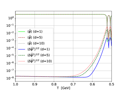
Figure 4: This plot shows the evolution of the mean and variance value. We chose the three different values of $d$ as $d=1$ (solid line), 5 (dashed line), and 10 (dotted line). Here, we chose $L=2\pi/(m_{\ast}a_{\ast})$.

Figure 4 shows the evolution of the homogeneous mode $\langle\tilde{\phi}\rangle$ and the root mean square of the fluctuation, $\langle\delta\tilde{\phi}^{2}\rangle^{1/2}$, where the brackets express the spatial average. Here, the simulation box size is set to $L=2\pi/(m_{\ast}a_{\ast})$, corresponding to $k_{\rm min}=m_{\ast}a_{\ast}$. While keeping $k_{\rm min,i}=k_{\rm min}$, we chose several different values of $k_{\rm max,i}$ by assigning the same field values for neighbor $d^{3}$ grids with $d=1,5,10$. This corresponds to introducing a UV cut-off of the initial spectrum at $k_{\rm max,i}=\pi/L\times N/d$. For a given $\sigma$, the initial amplitude of the field fluctuation $\delta\phi$ is given by $|\delta\phi|\sim\sigma/({\rm number~{}of~{}the~{}modes})^{1/2}$ with the number of the modes being roughly $(k_{\rm max,i}/k_{\rm min,i})^{3}\sim(N/d)^{3}$. Therefore, the maximum amplitude of the fluctuation increases as we increase $d$, correspondingly as we decrease $k_{\rm max,i}$, while the homogeneous mode is independent of $d$. As shown in Fig. 4, once the axion has started the oscillation, the exponential growth due to the tachyonic instability terminates, because the amplitude of the axion rapidly decreases due to the Hubble friction (a more detailed analysis can be found in Ref. [54]). As a result, before the inhomogeneity reaches ${\cal O}(1)$, the axion is settled down around the potential minimum, where the deviation from the quadratic potential is negligible.

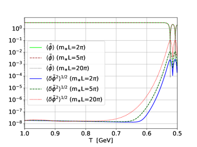
Figure 5: This plot shows the evolution of the mean and the variance value. We chose the three box size as $m_{\ast}L=2\pi$ (solid line), $m_{\ast}L=5\pi$ (dashed line), and $m_{\ast}L=20\pi$ (dotted line).

In Fig. 5, choosing $k_{\rm max,i}=k_{\rm max}=\pi N/L$, we have changed $k_{\rm min,i}=k_{\rm min}$ as $k_{\rm min,i}/(m_{\ast}a_{\ast})=1,\,2/5,1/10$ by choosing $m_{\ast}a_{\ast}L=2\pi,\,5\pi,\,20\pi$, respectively. As discussed in the previous subsection, the spatial gradient term disturbs the tachyonic instability, reducing the growth rate $\mu_{k}$. As we increase the box size, more and more low-$k$ modes, which undergo the tachyonic instability with the maximum growth rate $\mu_{k}\sim m(T)/m_{\ast}$ start to be included in the simulation. Therefore, the enhancement due to the tachyonic instability becomes more prominent for a larger box size. The $L$ dependence disappears, when we choose a sufficiently large $L$ so that the majority of the modes included in the simulation undergo the tachyonic instability, verifying that the result should not be altered by the change of the simulation setup.

Even for the largest simulation box with $m_{\ast}L=20\pi$, where the tachyonic instability becomes the most prominent, the instability has finished before the clump formation, being disturbed by the cosmic expansion. Here, we have chosen the size of the simulation box so that the minimum wavenumber becomes at most comparable to the Hubble scale. For example, for $m_{\ast}L=20\pi$, $k_{\rm min}$ amounts to $k_{\rm min}/(a_{\ast}H_{\ast})=0.3$. When we consider the super Hubble fluctuations, the metric perturbations, which are ignored in our computation, should be carefully considered.

3.3 Uncertainty at high temperature

In the previous subsection, we considered the cosine potential, which is predicted based on the DIGA. In Refs. [68, 63, 81, 82], it was shown that the DIGA well reproduces the lattice result in the high temperature range roughly above $T_{c}$. Meanwhile, it is known that for $T\geq{\cal O}(1)$ GeV, the lattice computation becomes rather challenging, because of the difficulty in sampling topologically non-trivial configurations. See Refs. [63, 83, 81, 84] for the recent studies about the lattice simulation in the high temperature range. Because of that, for $T\geq{\cal O}(1)$ GeV, the temperature dependence and the potential form of the axion have not been clearly understood as much as for $T<{\cal O}(1)$ GeV. Having considered this, in this subsection, we investigate whether the axion clump can be formed or not, when the temperature dependence of the axion mass or the potential form is modified for $T\geq{\cal O}(1)$ GeV.

First, we consider the case where the temperature dependence of $m$ becomes different for $T\geq T_{\ast\ast}=1.5$GeV as $m(T)\propto T^{-b_{\rm H}}$, while keeping $m(T)\propto T^{-b_{\rm L}}$ with $b_{\rm L}=8.7$ for $T\leq T_{\ast\ast}=1.5$GeV.

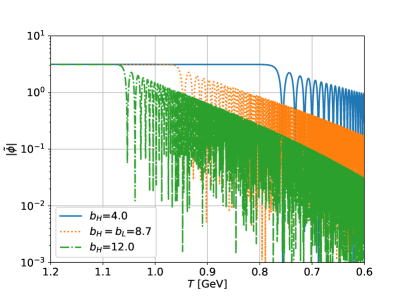
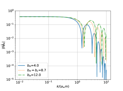
Figure 6: The left panel shows the evolution of background homogeneous mode for different $b_{H}$. Here, we set $b_{H}=4.0,8.7,12.0$, $T_{\ast\ast}=1.5$GeV, and $f=10^{11}$GeV. The right panel shows the spectrum for different $b_{H}$ when $|\delta\tilde{\phi}_{k}|$ has reached the maximum amplitude.

Figure 6 shows the evolution of the background field $\tilde{\phi}$ and the amplitude of the linear perturbation $\delta\tilde{\phi}_{k}$ for $b_{\rm H}=4.0,8.7,12.0$. Here we set the initial condition as Eqs. (3.4) and (3.5) and the decay constant as $f=10^{11}$GeV. The amplitude of $\delta\tilde{\phi}_{k}$ is evaluated at $t=t_{\ast}$, where $|\delta\tilde{\phi}_{k}|$ has reached the maximum value through the tacyonic growth. In Sec. 3.1, we argued that the temperature dependence of $m(T)$ does not significantly change the net enhancement due to the tachyonic instability. As is expected from this, the maximum amplitude of $\delta\tilde{\phi}_{k}$ remains almost the same, even if we change the value of $b_{\rm H}$.

Our next target is considering the case where the potential form is modified from Eq. (2.2) at $T\geq T_{\ast\ast}=1.5$GeV. Here, instead of considering a modified potential directly, we consider a modification of the initial velocity as $d\tilde{\phi}/d\tilde{t}|_{\tilde{t}_{i}=\tilde{t}_{\ast\ast}}=d\tilde{\phi}/d\tilde{t}|_{{\rm SR}}\times 10^{c}$ choosing the initial time as $\tilde{t}_{\ast\ast}=\tilde{t}(T_{\ast\ast})$, where $d\tilde{\phi}/d\tilde{t}|_{{\rm SR}}$ denotes the initial velocity determined by imposing the slow-roll condition, (3.5). Choosing $c<0$ ($c>0$) corresponds to considering the case where the axion was initially located at a shallower (steeper) potential region than Eq. (2.2) under the slow-roll condition.

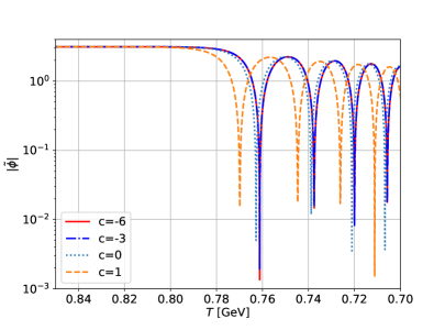
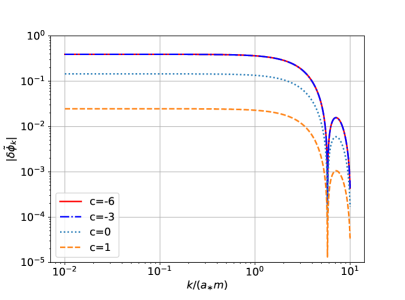
Figure 7: The left panel shows the evolution of background homogeneous mode and the right panel shows the spectrum when $|\delta\tilde{\phi}_{k}|$ has reached the maximum amplitude. Here, we set $c$ to $c=-6,-3,0,1$.

Figure 7 shows the evolution of the background field $\tilde{\phi}$ and the amplitude of the linear perturbation $\delta\tilde{\phi}_{k}$ for $c=-6,-3,0,1$. Again, we set the initial condition as Eqs. (3.4) and (3.5) and the decay constant as $f=10^{11}$GeV. For $c<0$, the enhancement due to the tachyonic instability becomes slightly larger than $c=0$, addressed in the previous subsection. However, even with this modification, the tachyonic instability terminates before the inhomogeneity $|\delta\tilde{\phi}_{k}|$, which roughly amounts to $|\delta\phi/\phi|$, becomes ${\cal O}(1)$. This is because the sustainability of the tachyonic instability is mainly determined by the dynamics around $T=T_{\ast}$.

In this section, we have shown that the inhomogeneity of the axion grows exponentially due to the tachyonic instability. Nevertheless, the enhancement has turned out to be insufficient for the axion clump formation in the pre-inflationary scenario, verifying the prevailing understanding.

4 Clump formation: ALPs

In the previous section, focusing on QCD axion, we showed that the tachyonic instability is not enough for the clump formation in the scenario where the PQ symmetry breaking takes place before or during inflation. In this section, we investigate the possibility of the clump formation for ALPs, which can have a more general form of the potential. There are only few studies about ALP clump formation in the pre-inflationary scenario. In Ref. [85], Hardy considered a scenario where a hidden sector from which an ALP acquires the mass undergoes the first order phase transition. As a consequence, it was argued that the ALP mass inside formed bubbles becomes larger than the one outside bubbles. The difference in the ALP mass results in the difference in the commencement time of the oscillation, generating the inhomogeneity of the energy density due to the difference in the dilution factor. In Refs. [54, 86], it was shown that when the ALP potential has an extensive shallow region likewise the potential proposed in Ref. [87], the parametric resonance becomes rather efficient, leading to ${\cal O}(1)$ inhomogeneity [54] and subsequently to the formation of overdense clumps [86], called oscillons, also in the pre-inflationary scenario. Since the potential addressed in Refs. [54, 86] is very different from the cosine potential, one may wonder whether a similar situation can be realized just with a milder modification from the conventional cosine potential. In this section, we investigate the possibility of ALP clump formation for a potential with multiple cosine terms, presented in 2.2.

4.1 Linear calculation

In this section, we investigate whether the ALP fluctuation can be saturated to the background homogeneous mode, considering the potential (2.9) with several different values of $\epsilon$. When the value of $\epsilon$ is close to zero, the top of the potential becomes flatter (see $\epsilon=0.01$ in Fig. 1.). Then, the low-$k$ modes of $\delta\tilde{\phi}_{k}$ can stay long in the tachyonic region, growing exponentially. Furthermore, when the ALP is located at a shallow potential region before the commencement of the oscillation, the parametric resonance sustains longer, since the delay of the onset of the oscillation makes the effect of the cosmic expansion less effective. Changing the initial condition and the potential parameter $\epsilon$, we consider the instabilities classified into the following three categories:

$$|\delta{\phi}/\phi|\ {\rm becomes}\ {\cal O}(1)\ {\rm by}=\begin{cases}{\rm tachyonic\ instability}&{\rm(i)}\\ {\rm tachyonic\ instability\ \&\ parametric\ resonance}&{\rm(ii)}\\ {\rm parametric\ resonance}&{\rm(iii)}\end{cases}$$

one by one.

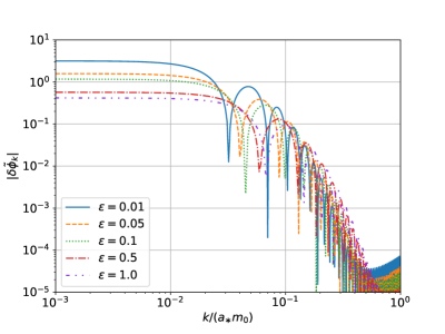
Figure 8: This plot shows the spectrum of the ALP field fluctuation for the potential (2.9) with $\epsilon$=0.01 (blue solid), 0.05 (orange dashed), 0.1 (green dotted), 0.5 (red dash-dotted), and 1.0 (purple dash-dot-dotted), respectively. Each spectrum is evaluated, when the amplitude has reached the maximum value. Here, the initial condition is set as $\tilde{\phi}_{i}=2\pi\times(1-10^{-7})$ and $\delta\tilde{\phi}_{k,i}=2\pi\times 10^{-8}$ at $\tilde{T}_{i}=5.0$. In this case, the ALP fluctuation is solely enhanced by the tachyonic instability (type (i)). For $\epsilon=0.01,\,0.05,\,0.1$, since $|\delta\tilde{\phi}_{k}|$, which roughly corresponds to $|\delta\phi/\phi|$, reaches ${\cal O}(1)$, the computation based on the linear analysis is not reliable.

4.1.1 Type i: Tachyonic instability

When we consider the case where $\phi$ is tuned around the top of the potential ($\tilde{\phi}\simeq 2\pi$) before the onset of the oscillation, the tachyonic instability can enhance the inhomogeneity of the ALP field. We have numerically followed the evolution of each Fourier mode of field fluctuation together with the background field. We start our calculation at $\tilde{T}_{*}=T_{*}/T_{c}$. In what follows, we express $\tilde{\phi}$ and $\delta\tilde{\phi}$ evaluated at $T=T_{*}$ as

$$\tilde{\phi}_{i}\equiv\tilde{\phi}(T_{*})\,,\qquad\quad\delta\tilde{\phi}_{k,i}\equiv\delta\tilde{\phi}_{k}(T_{*})$$ (4.1)

For $\tilde{T}_{*}\ll 1$ or equivalently $T_{*}\ll T_{c}$, the ALP mass remains constant. On the other hand, for $\tilde{T}_{*}\geq 1$ or $T_{*}\geq T_{c}$, $m(T)$ varies as the temperature decreases during the oscillation.

Figure 8 shows the resultant spectrum of $\delta\tilde{\phi}_{k}$ for five different values of $\epsilon$, evaluated when the fluctuation has reached the maximum amplitude. Here, we set $b=8.0$ and employ the initial condition for the background and fluctuation as

$$\tilde{\phi}_{i}=2\pi\times(1-10^{-7})\,,\qquad\delta\tilde{\phi}_{k,i}=2\pi\times 10^{-8}\,,$$ (4.2)

at $\tilde{T}_{*}=5.0$. Since the dominant instability is the tachyonic instability, all the low $k$ modes are uniformly enhanced. In the previous section, for the QCD axion with the cosine potential, we showed that the tachyonic instability terminates before $|\delta\phi/\phi|$ reaches ${\cal O}(1)$, since the axion field rapidly rolls down the potential, exiting the negative curvature region of the potential. For the potential (2.9) with $\epsilon<1$, since the gradient of the potential around the hilltop is shallower than the one for the cosine potential, the tachyonic instability continues longer. As a result, when $\tilde{\phi}_{i}$ is tuned around $\pi$, $|\delta\phi/\phi|$ can reach ${\cal O}(1)$ only through the exponential growth due to the tachyonic instability. For $\epsilon=0.01,\,0.05,\,0.1$, since $|\delta\tilde{\phi}_{k}|$, which roughly corresponds to $|\delta\phi/\phi|$, is enhanced to be ${\cal O}(1)$, we need to take into account the non-linearity to compute the dynamics properly.

When the ALP fluctuation is significantly enhanced by the tachyonic instability, we also need to make sure that this does not contradict to the isocurvature constraint in the CMB scales [88]. To solve the super Hubble evolution, we also need to take into account the metric perturbations, which are ignored in this paper. The impact of the self-interaction on the isocurvature constraint was discussed in Ref. [42].

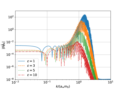
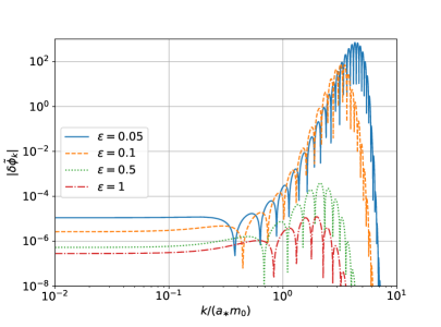
Figure 9: The left panel shows the spectrum for $\epsilon$=1 (blue solid), 3 (orange dashed), 5 (green dotted), 10 (red dash-dotted). The initial condition is given by $\tilde{\phi}_{i}=2\pi\times(1-10^{-5})$ and $\delta\tilde{\phi}_{i}=2\pi\times 10^{-8}$ at $\tilde{T}_{*}=T_{*}/T_{c}=5.0$. In this case, the inhomogeneity becomes ${\cal O}(1)$ through the tachyonic instability and the succeeding resonance instability (type (ii)). The right panel shows the spectrum for $\epsilon$=0.05 (blue solid), 0.1 (orange dashed), 0.5 (green dotted), 1 (red dash-dotted). The initial condition is set by $\tilde{\phi}_{i}=2\pi\times(1-10^{-2})$ and $\delta\tilde{\phi}_{k,i}=2\pi\times 10^{-8}$ at $\tilde{T}_{i}=0.5$. In this case, the inhomogeneity becomes ${\cal O}(1)$ solely through the resonance instability (type (iii)). For $\epsilon=5,10$ in the left panel and for $\epsilon=0.5,1$ in the right panel, the spectra are evaluated, when they have reached the maximum values, while for the rest, they are evaluated right after $|\delta\tilde{\phi}_{k}|$ has reached ${\cal O}(1)$, where the non-linear analysis is required.

4.1.2 Type ii: Tachyonic & Parametric resonance instabilities

When $\phi_{i}$ is not fine-tuned around a shallow potential region as much as type (i), the tachyonic instability finishes before the inhomogeneity becomes ${\cal O}(1)$. Nevertheless, in some cases, the tachyonic instability is followed by the resonance instability. In the end, the amplitude of $\delta\phi/\phi$ can reach ${\cal O}(1)$ through the tachyonic instability and the succeeding resonance instability.

The left panel of Fig. 9 shows the spectrum for $\epsilon=1$ (blue solid), $\epsilon=3$ (orange dashed), $\epsilon=5$ (green dotted), $\epsilon=10$ (red dash-dotted). The initial values of the background and each Fourier mode are set as

$$\tilde{\phi}_{i}=2\pi\times(1-10^{-5})\,,\qquad\delta\tilde{\phi}_{k,i}=2\pi\times 10^{-8}\,,$$ (4.3)

at $\tilde{T}_{*}=5$. After the low-$k$ modes are enhanced by the tachyonic instability, the resonance instability creates a peak in the spectrum corresponding to the first resonance band. We will discuss the time evolution in more detail in the next subsection.

4.1.3 Type iii: Resonance instability

In general, when the frequency of the oscillation, $\omega$, significantly changes in time, taking $|\dot{\omega}/\omega^{2}|\geq{\cal O}(1)$, a sustainable parametric resonance hardly takes place. Meanwhile, for $T_{*}\ll T_{c}$, $m(T)$ has already stopped evolving, when the ALP commences the oscillation. In that case, the parametric resonance can efficiently enhance the inhomogeneous mode of $\phi$ during the oscillation. In addition, when the oscillation starts much later than the time $t=t_{\ast}$ with $3H_{\ast}=m_{\ast}$, the time scale of the oscillation is much shorter than the one of the cosmic expansion already just after the commencement of the oscillation. In this case, the sustained parametric resonance can take place without being disturbed by the cosmic expansion. As discussed in Refs. [60, 54], the delayed onset is characterized by

$$H_{\rm osc}\sim\sqrt{|(dV(\phi_{i})/d\phi_{i})/\phi_{i}|}\quad{\rm or}\quad H_{\rm osc}/m\sim\sqrt{|(d\tilde{V}(\tilde{\phi}_{i})/d\tilde{\phi}_{i})/\tilde{\phi}_{i}|}\,,$$ (4.4)

when $\phi$ is not the dominant component of the Universe (see Ref. [62] about the evaluation of $H_{\rm osc}/m$ when $\phi$ is the dominant component). Therefore, when $\phi$ was initially located at a potential region where the gradient is shallower than the one for the quadratic one, the oscillation starts much later than $t=t_{\ast}$, leading to the efficient parametric resonance.

The right panel of Fig. 9 shows the spectrum for $\epsilon=0.05$ (blue solid), 0.1 (orange dashed), 0.5 (green dotted), 1 (red dash-dotted). The initial condition is set as

$$\tilde{\phi}_{i}=2\pi\times(1-10^{-2})\,,\qquad\delta\tilde{\phi}_{k,i}=2\pi\times 10^{-8}\,,$$ (4.5)

at $\tilde{T}_{*}=0.5$. In these cases, while the tachyonic instability does not persist, the succeeding resonance instability leads to the ${\cal O}(1)$ inhomogeneity. As a result, the resonance instability creates a peak around the first resonance band. This case was addressed in Refs. [54, 86].

4.2 Nonlinear calculation

As discussed in the previous subsection, even if we start with an almost homogeneous initial condition, corresponding to the case where the symmetry breaking takes place before or during inflation, the tachyonic instability and/or the resonance instability can enhance the inhomogeneity to be $|\delta\phi/\phi|\sim{\cal O}(1)$. In this case, the dynamics cannot be described by the linear analysis. In this subsection, we solve the Klein-Gordon equation (2.12) for the potential (2.9), using (3+1) dimensional lattice simulation with $128^{3}$ grids. We consider three examples that correspond to type (i), (ii) and (iii), respectively, as summarized in Table 1.

Table 1: Simulation setup

Type	$\langle\tilde{\phi}_{i}\rangle$	$\langle\delta\tilde{\phi}^{2}\rangle^{1/2}$	$\epsilon$	$\tilde{T}_{*}$	$m_{0}L$
(i)	$2\pi\times(1-10^{-9})$	$2\pi\times 10^{-8}$	0.01	5	$4\pi$
(ii)	$2\pi\times(1-10^{-7})$	$2\pi\times 10^{-8}$	0.05	5	$2\pi$
(iii)	$2\pi\times(1-10^{-2})$	$2\pi\times 10^{-8}$	0.05	0.5	$2\pi$

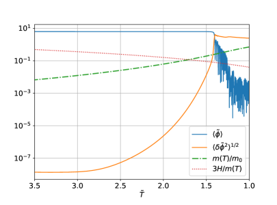
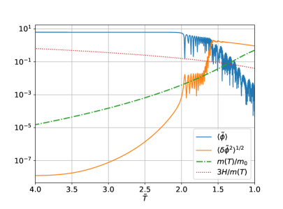
Figure 10: These plots show the evolution of the spatial average of $\tilde{\phi}$(blue), the root-mean-square of field fluctuation $\langle\delta\tilde{\phi}^{2}\rangle^{1/2}$(orange), $m(T)/m_{0}$ (green dashed), and $3H/m(T)$. The left and right panels are for the type (i) and (ii), respectively.

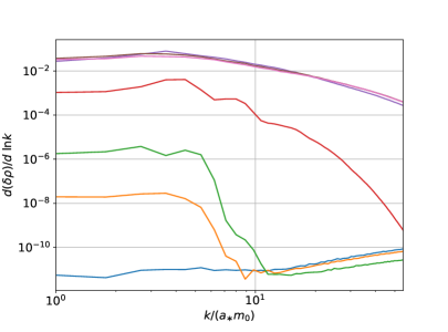
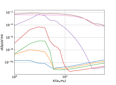
Figure 11: The left and right panels show the evolution of the energy density fluctuation for type (i) and (iii). Time evolves from bottom to top.

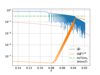
Figure 12: Same as Fig. 10 but for type (iii).

4.2.1 Type i: Tachyonic instability

As type (i), we consider the case where the inhomogeneity grows solely due to the tachypnic isntability. The left panel of Fig. 10 shows the evolution of the homogeneous mode (blue) and the root-mean-square of the fluctuation (orange). In type (i), the fluctuation grows exponentially due to the tachyonic instability. The green dotted line shows the time variation of the ALP mass. As the inhomogeneity grows, the spatial gradient term that disturbs the tachyonic growth becomes more prominent. When the amplitude of the inhomogeneous fluctuation becomes comparable to the homogeneous one, the tachyonic growth terminates.

The left panel of Fig. 11 shows the evolution of the spectrum of the energy density. Different colours show spectra evaluated at different times. Figure 13 shows the snapshot of the time evolution of the energy density distribution. As is shown, the tachyonic instability leads to the formation of a number of ALP clumps, which is also known as the oscillon. Usually, oscillons are formed through the parametric resonance instability. Here, we have shown that ALP oscillons can be formed through the tachyonic instability only.

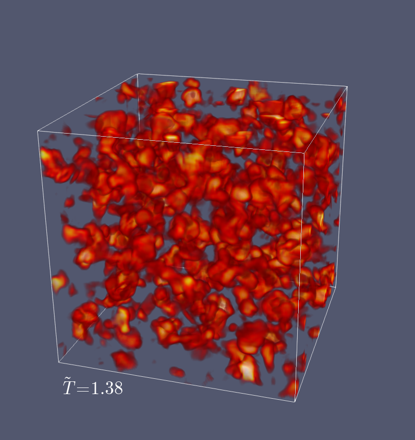
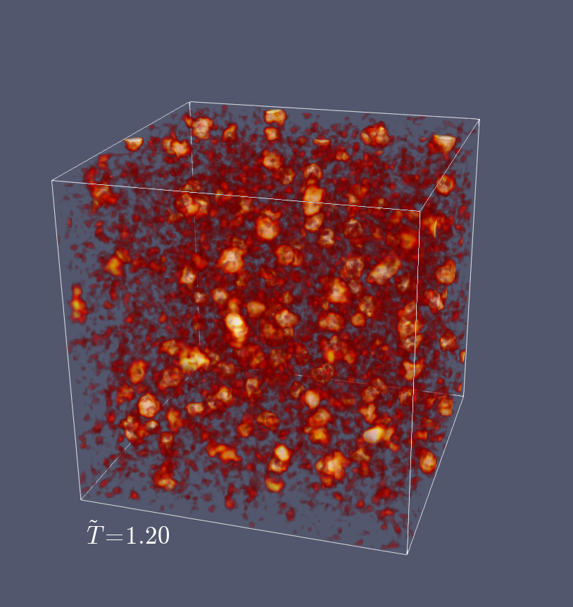
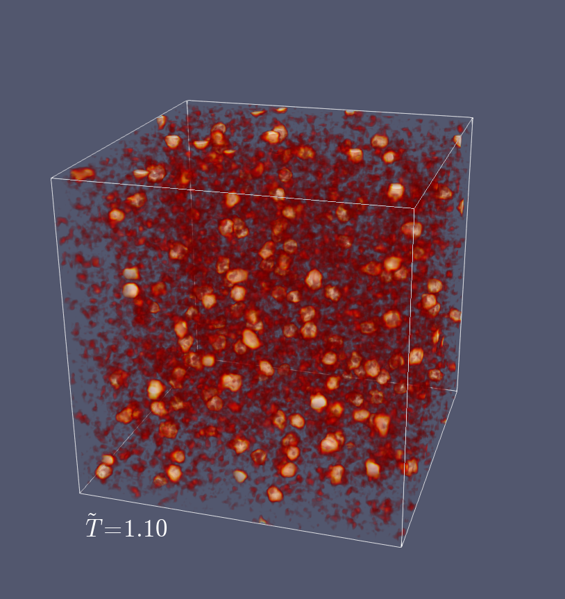
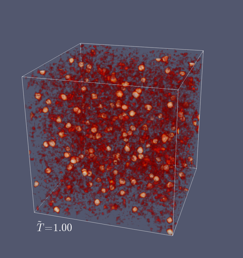
Figure 13: Snapshot of the evolution of the axion energy density evaluated at $\tilde{T}=$1.38, 1.20, 1.10 and 1.00 for type (i). The red and yellow region correspond to $\rho/\langle\rho\rangle>2$ and 4 respectively.

4.2.2 Type ii: Tachyonic & Resonance instability

Next, we consider an example of type (ii), where the fluctuation grows due to both the tahyonic instability and the resonance instability. In this case, after the tachyonic instability stops being effective, the fluctuation starts to grow subsequently due to the resonance instability. The right panel of Fig. 10 shows the time evolution of the homogeneous and inhomogeneous modes of $\phi$. As shown by the green dotted line, the exponential growth due to the resonance instability takes place also during the ALP mass keeps on growing. This is possible because when the resonance instability started, the time scale of the oscillation has become shorter than the one of the variation of $m(T)$, which is of order of the time scale of the cosmic expansion.

As shown in Fig. 10, the fluctuation once stops growing for a while around $\tilde{T}\sim 2.0$. This is because the Fourier modes enhanced by the tachyonic instability differ from those enhanced by the resonance instability. The first stage of the growth is driven by the former and the second stage is driven by the latter. When the tachyonic growth terminated and the resonance instability set in, the contributions from the modes in the resonance band are still subdominant, compared to those enhanced by the tachyonic instability. Therefore, their exponential growth is not visible in the spatial average of the squared fluctuation, which sums up all the modes in the simulation. Finally, the exponential growth due to the resonance terminates, when the inhomogeneity becomes ${\cal O}(1)$ and the backreaction turns on.

4.2.3 Type iii: Resonance instability

For $T_{*}/T_{c}\ll 1$, when the ALP started the oscillation, $m(T)$ had already settled down at the constant value, $m_{0}$. The coherent oscillation with the constant period leads to the parametric resonance as discussed in the previous subsection based on the linear analysis. Figure 12 shows the time evolution of the homogeneous and inhomogeneous modes of $\phi$. Also in this case, the backreaction terminates the exponential growth due to the parametric resonance.

The right panel of Fig. 11 shows the evolution of the spectrum of the energy density. Figure 14 shows the snapshot of the energy density. The resonance instablity also leads to the formation of a number of oscillons made of the oscillating ALP field. In Fig. 13, the size of the oscillons is much smaller than the one in Fig. 14. This is because the typical length scale of the system $1/m$ becomes smaller and smaller due to the increasing mass for type (i).

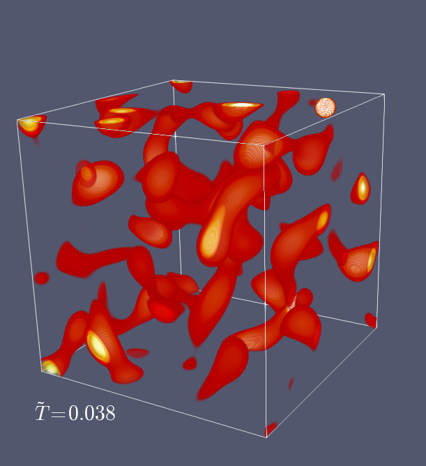
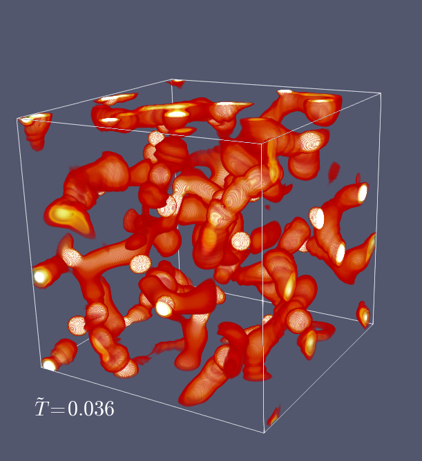
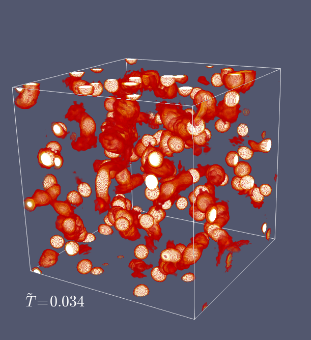
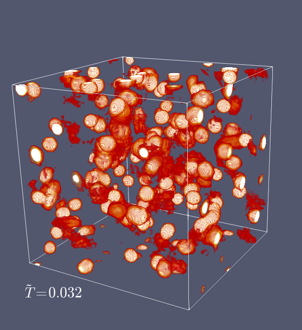
Figure 14: Snapshot of the evolution of the axion energy density evaluated at $\tilde{T}=0.038$, 0.036, 0.034, and 0.032 for type (iii). The red and yellow region correspond to $\rho/\langle\rho\rangle>2$ and 4, respectively.

5 Conclusion

In this paper, we investigated the possibility of clump formation for QCD axion and ALPs, considering the case where the PQ symmetry was already broken during inflation. For the QCD axion, while the inhomogeneity grows exponentially due to the tachyonic instability, it turned out that fluctuation does not grow sufficiently to become ${\cal O}(1)$, even for a fine-tuned initial condition. Therefore, a future discovery of the QCD axion clump strongly suggests that the PQ symmetry was broken after inflation, verifying the prevailing understanding.

Meanwhile, for ALPs, the axion clumps or the oscillons can be formed through: (i) the tachyonic instability, (ii) the tachyonic instability and the parametric resonance instability, and (iii) the parametric resonance instability. In most of the existing studies, the oscillons are formed as a consequence of the resonance instability. In this paper, we pointed out that the oscillons can be formed through the tachyonic instability only.

In order to discuss a possible phenomenological consequence of ALP clumps or ALP oscillons, we need to understand their lifetime. According to numerical simulations, it has been known that oscillons are typically long-lived. In Ref. [89], it was shown that the longevity of oscillons can be understood from an approximate U(1) symmetry, which is realized in the non-relativistic limit. The approximate symmetry correspondingly ensures an approximate conservation of particle number. Meanwhile, oscillons are not absolutely stable. As discussed in Refs. [90, 41], the decay of oscillons is caused by a deviation from the quadratic potential, that leads to a classical emission of relativistic particles, violating the number conservation. It is interesting to see whether the lifetime of osciilons differs among type (i), (ii), and (iii). We will report this analysis in our forthcoming paper.

References

- [1] B. Graner, Y. Chen, E. G. Lindahl and B. R. Heckel, Reduced Limit on the Permanent Electric Dipole Moment of Hg199, Phys. Rev. Lett. 116 (2016) 161601 [1601.04339].
- [2] R. D. Peccei and H. R. Quinn, CP Conservation in the Presence of Instantons, Phys. Rev. Lett. 38 (1977) 1440.
- [3] R. D. Peccei and H. R. Quinn, Constraints Imposed by CP Conservation in the Presence of Instantons, Phys. Rev. D16 (1977) 1791.
- [4] S. Weinberg, A New Light Boson?, Phys. Rev. Lett. 40 (1978) 223.
- [5] F. Wilczek, Problem of Strong and Invariance in the Presence of Instantons, Phys. Rev. Lett. 40 (1978) 279.
- [6] J. E. Kim, Weak Interaction Singlet and Strong CP Invariance, Phys. Rev. Lett. 43 (1979) 103.
- [7] M. A. Shifman, A. I. Vainshtein and V. I. Zakharov, QCD and Resonance Physics. Theoretical Foundations, Nucl. Phys. B147 (1979) 385.
- [8] M. Dine, W. Fischler and M. Srednicki, A Simple Solution to the Strong CP Problem with a Harmless Axion, Phys. Lett. 104B (1981) 199.
- [9] A. Zhitnitsky, On possible suppression of the axion-hadron interactions, Sov. J. Nucl. Phys. 31 (1980) 260.
- [10] J. Preskill, M. B. Wise and F. Wilczek, Cosmology of the Invisible Axion, Phys. Lett. 120B (1983) 127.
- [11] L. F. Abbott and P. Sikivie, A Cosmological Bound on the Invisible Axion, Phys. Lett. 120B (1983) 133.
- [12] M. Dine and W. Fischler, The Not So Harmless Axion, Phys. Lett. 120B (1983) 137.
- [13] P. Sikivie, Axion Cosmology, Lect. Notes Phys. 741 (2008) 19 [astro-ph/0610440].
- [14] D. J. E. Marsh, Axion Cosmology, Phys. Rept. 643 (2016) 1 [1510.07633].
- [15] I. G. Irastorza and J. Redondo, New experimental approaches in the search for axion-like particles, Prog. Part. Nucl. Phys. 102 (2018) 89 [1801.08127].
- [16] P. Sikivie, Of Axions, Domain Walls and the Early Universe, Phys. Rev. Lett. 48 (1982) 1156.
- [17] E. W. Kolb and I. I. Tkachev, Axion miniclusters and Bose stars, Phys. Rev. Lett. 71 (1993) 3051 [hep-ph/9303313].
- [18] E. W. Kolb and I. I. Tkachev, Nonlinear axion dynamics and formation of cosmological pseudosolitons, Phys. Rev. D49 (1994) 5040 [astro-ph/9311037].
- [19] E. W. Kolb and I. I. Tkachev, Large amplitude isothermal fluctuations and high density dark matter clumps, Phys. Rev. D50 (1994) 769 [astro-ph/9403011].
- [20] C. J. Hogan and M. J. Rees, AXION MINICLUSTERS, Phys. Lett. B205 (1988) 228.
- [21] K. M. Zurek, C. J. Hogan and T. R. Quinn, Astrophysical Effects of Scalar Dark Matter Miniclusters, Phys. Rev. D75 (2007) 043511 [astro-ph/0607341].
- [22] B. Eggemeier, J. Redondo, K. Dolag, J. C. Niemeyer and A. Vaquero, First simulations of axion minicluster halos, 1911.09417.
- [23] P. Tinyakov, I. Tkachev and K. Zioutas, Tidal streams from axion miniclusters and direct axion searches, JCAP 1601 (2016) 035 [1512.02884].
- [24] J. Enander, A. Pargner and T. Schwetz, Axion minicluster power spectrum and mass function, JCAP 12 (2017) 038 [1708.04466].
- [25] I. Tkachev, Phenomenology of Axion Miniclusters, in Proceedings, 11th Patras Workshop on Axions, WIMPs and WISPs (Axion-WIMP 2015): Zaragoza, Spain, June 22-26, 2015, pp. 173–178, 2015, DOI.
- [26] E. Seidel and W.-M. Suen, Formation of solitonic stars through gravitational cooling, Phys. Rev. Lett. 72 (1994) 2516 [gr-qc/9309015].
- [27] E. Braaten, A. Mohapatra and H. Zhang, Dense Axion Stars, Phys. Rev. Lett. 117 (2016) 121801 [1512.00108].
- [28] D. G. Levkov, A. G. Panin and I. I. Tkachev, Relativistic axions from collapsing Bose stars, Phys. Rev. Lett. 118 (2017) 011301 [1609.03611].
- [29] L. Visinelli, S. Baum, J. Redondo, K. Freese and F. Wilczek, Dilute and dense axion stars, Phys. Lett. B777 (2018) 64 [1710.08910].
- [30] J. C. Niemeyer, Small-scale structure of fuzzy and axion-like dark matter, 1912.07064.
- [31] E. W. Kolb and I. I. Tkachev, Femtolensing and picolensing by axion miniclusters, Astrophys. J. 460 (1996) L25 [astro-ph/9510043].
- [32] M. Fairbairn, D. J. E. Marsh and J. Quevillon, Searching for the QCD Axion with Gravitational Microlensing, Phys. Rev. Lett. 119 (2017) 021101 [1701.04787].
- [33] M. Fairbairn, D. J. E. Marsh, J. Quevillon and S. Rozier, Structure formation and microlensing with axion miniclusters, Phys. Rev. D97 (2018) 083502 [1707.03310].
- [34] L. Dai and J. Miralda-Escudé, Gravitational Lensing Signatures of Axion Dark Matter Minihalos in Highly Magnified Stars, Astron. J. 159 (2020) 49 [1908.01773].
- [35] M. Gleiser, Pseudostable bubbles, Physical Review D 49 (1994) 2978.
- [36] P. Salmi and M. Hindmarsh, Radiation and Relaxation of Oscillons, Phys. Rev. D85 (2012) 085033 [1201.1934].
- [37] E. J. Copeland, M. Gleiser and H.-R. Müller, Oscillons: Resonant configurations during bubble collapse, Physical Review D 52 (1995) 1920.
- [38] M. A. Amin, R. Easther and H. Finkel, Inflaton fragmentation and oscillon formation in three dimensions, Journal of Cosmology and Astroparticle Physics 2010 (2010) 001.
- [39] M. A. Amin, R. Easther, H. Finkel, R. Flauger and M. P. Hertzberg, Oscillons after inflation, Physical Review Letters 108 (2012) .
- [40] K. D. Lozanov and M. A. Amin, Self-resonance after inflation: Oscillons, transients, and radiation domination, Physical Review D 97 (2018) .
- [41] J. Ollé, O. Pujolàs and F. Rompineve, Oscillons and Dark Matter, JCAP 2002 (2020) 006 [1906.06352].
- [42] T. Kobayashi, R. Kurematsu and F. Takahashi, Isocurvature Constraints and Anharmonic Effects on QCD Axion Dark Matter, JCAP 1309 (2013) 032 [1304.0922].
- [43] A. A. Starobinsky, Dynamics of Phase Transition in the New Inflationary Universe Scenario and Generation of Perturbations, Phys. Lett. 117B (1982) 175.
- [44] M. Sasaki and E. D. Stewart, A General analytic formula for the spectral index of the density perturbations produced during inflation, Prog. Theor. Phys. 95 (1996) 71 [astro-ph/9507001].
- [45] M. Sasaki and T. Tanaka, Superhorizon scale dynamics of multiscalar inflation, Prog. Theor. Phys. 99 (1998) 763 [gr-qc/9801017].
- [46] R. T. Co, E. Gonzalez and K. Harigaya, Axion Misalignment Driven to the Hilltop, JHEP 05 (2019) 163 [1812.11192].
- [47] E. Witten, Some Properties of O(32) Superstrings, Phys. Lett. 149B (1984) 351.
- [48] P. Svrcek and E. Witten, Axions In String Theory, JHEP 06 (2006) 051 [hep-th/0605206].
- [49] A. Arvanitaki, S. Dimopoulos, S. Dubovsky, N. Kaloper and J. March-Russell, String Axiverse, Phys. Rev. D81 (2010) 123530 [0905.4720].
- [50] M. Czerny and F. Takahashi, Multi-Natural Inflation, Phys. Lett. B733 (2014) 241 [1401.5212].
- [51] M. Czerny, T. Higaki and F. Takahashi, Multi-Natural Inflation in Supergravity, JHEP 05 (2014) 144 [1403.0410].
- [52] P. B. Greene, L. Kofman and A. A. Starobinsky, Sine-Gordon parametric resonance, Nucl. Phys. B543 (1999) 423 [hep-ph/9808477].
- [53] J. Soda and Y. Urakawa, Cosmological imprints of string axions in plateau, Eur. Phys. J. C78 (2018) 779 [1710.00305].
- [54] H. Fukunaga, N. Kitajima and Y. Urakawa, Efficient self-resonance instability from axions, Journal of Cosmology and Astroparticle Physics 2019 (2019) 055.
- [55] S.-Y. Zhou, E. J. Copeland, R. Easther, H. Finkel, Z.-G. Mou and P. M. Saffin, Gravitational Waves from Oscillon Preheating, JHEP 10 (2013) 026 [1304.6094].
- [56] S. Antusch, F. Cefala and S. Orani, Gravitational waves from oscillons after inflation, Phys. Rev. Lett. 118 (2017) 011303 [1607.01314].
- [57] J. Liu, Z.-K. Guo, R.-G. Cai and G. Shiu, Gravitational Waves from Oscillons with Cuspy Potentials, Phys. Rev. Lett. 120 (2018) 031301 [1707.09841].
- [58] S. Antusch, F. Cefala and S. Orani, What can we learn from the stochastic gravitational wave background produced by oscillons?, JCAP 1803 (2018) 032 [1712.03231].
- [59] S. Antusch, F. Cefala, S. Krippendorf, F. Muia, S. Orani and F. Quevedo, Oscillons from String Moduli, JHEP 01 (2018) 083 [1708.08922].
- [60] N. Kitajima, J. Soda and Y. Urakawa, Gravitational wave forest from string axiverse, JCAP 1810 (2018) 008 [1807.07037].
- [61] P. Adshead, J. T. Giblin, T. R. Scully and E. I. Sfakianakis, Magnetogenesis from axion inflation, JCAP 1610 (2016) 039 [1606.08474].
- [62] T. Patel, H. Tashiro and Y. Urakawa, Resonant magnetogenesis from axions, JCAP 2001 (2020) 043 [1909.00288].
- [63] S. Borsanyi et al., Lattice QCD for Cosmology, Nature 539 (2016) 69 [1606.07494].
- [64] P. Di Vecchia and G. Veneziano, Chiral Dynamics in the Large n Limit, Nucl. Phys. B171 (1980) 253.
- [65] G. Grilli di Cortona, E. Hardy, J. Pardo Vega and G. Villadoro, The QCD axion, precisely, JHEP 01 (2016) 034 [1511.02867].
- [66] P. Fox, A. Pierce and S. D. Thomas, Probing a QCD string axion with precision cosmological measurements, hep-th/0409059.
- [67] E. Berkowitz, M. I. Buchoff and E. Rinaldi, Lattice QCD input for axion cosmology, Phys. Rev. D92 (2015) 034507 [1505.07455].
- [68] S. Borsanyi, M. Dierigl, Z. Fodor, S. D. Katz, S. W. Mages, D. Nogradi et al., Axion cosmology, lattice QCD and the dilute instanton gas, Phys. Lett. B752 (2016) 175 [1508.06917].
- [69] M. S. Turner, Cosmic and Local Mass Density of Invisible Axions, Phys. Rev. D33 (1986) 889.
- [70] L. Visinelli and P. Gondolo, Dark Matter Axions Revisited, Phys. Rev. D 80 (2009) 035024 [0903.4377].
- [71] D. H. Lyth, Axions and inflation: Sitting in the vacuum, Phys. Rev. D45 (1992) 3394.
- [72] K. J. Bae, J.-H. Huh and J. E. Kim, Update of axion CDM energy, JCAP 0809 (2008) 005 [0806.0497].
- [73] L. Abbott and P. Sikivie, A cosmological bound on the invisible axion, Physics Letters B 120 (1983) 133 .
- [74] R. Mayle, J. R. Wilson, J. R. Ellis, K. A. Olive, D. N. Schramm and G. Steigman, Constraints on Axions from SN 1987a, Phys. Lett. B203 (1988) 188.
- [75] J. E. Kim, H. P. Nilles and M. Peloso, Completing natural inflation, JCAP 0501 (2005) 005 [hep-ph/0409138].
- [76] M. Peloso and C. Unal, Trajectories with suppressed tensor-to-scalar ratio in Aligned Natural Inflation, JCAP 1506 (2015) 040 [1504.02784].
- [77] S. R. Coleman, Q Balls, Nucl. Phys. B262 (1985) 263.
- [78] A. Kusenko and M. E. Shaposhnikov, Supersymmetric Q balls as dark matter, Phys. Lett. B418 (1998) 46 [hep-ph/9709492].
- [79] S. Kasuya and M. Kawasaki, Q ball formation through Affleck-Dine mechanism, Phys. Rev. D61 (2000) 041301 [hep-ph/9909509].
- [80] T. Hiramatsu, M. Kawasaki and F. Takahashi, Numerical study of Q-ball formation in gravity mediation, JCAP 1006 (2010) 008 [1003.1779].
- [81] Y. Taniguchi, K. Kanaya, H. Suzuki and T. Umeda, Topological susceptibility in finite temperature ( 2+1 )-flavor QCD using gradient flow, Phys. Rev. D95 (2017) 054502 [1611.02411].
- [82] P. Petreczky, H.-P. Schadler and S. Sharma, The topological susceptibility in finite temperature QCD and axion cosmology, Phys. Lett. B762 (2016) 498 [1606.03145].
- [83] J. Frison, R. Kitano, H. Matsufuru, S. Mori and N. Yamada, Topological susceptibility at high temperature on the lattice, JHEP 09 (2016) 021 [1606.07175].
- [84] P. T. Jahn, G. D. Moore and D. Robaina, Topological Susceptibility to High Temperatures via Reweighting, PoS LATTICE2018 (2018) 155 [1810.13218].
- [85] E. Hardy, Miniclusters in the Axiverse, JHEP 02 (2017) 046 [1609.00208].
- [86] M. Kawasaki, W. Nakano and E. Sonomoto, Oscillon of Ultra-Light Axion-like Particle, JCAP 2001 (2020) 047 [1909.10805].
- [87] Y. Nomura, T. Watari and M. Yamazaki, Pure Natural Inflation, Phys. Lett. B776 (2018) 227 [1706.08522].
- [88] Planck collaboration, Planck 2018 results. X. Constraints on inflation, 1807.06211.
- [89] K. Mukaida, M. Takimoto and M. Yamada, On Longevity of I-ball/Oscillon, JHEP 03 (2017) 122 [1612.07750].
- [90] M. Ibe, M. Kawasaki, W. Nakano and E. Sonomoto, Decay of I-ball/Oscillon in Classical Field Theory, JHEP 04 (2019) 030 [1901.06130].