A New Smoothing Algorithm for
Jump Markov Linear Systems

Abstract

This paper presents a method for calculating the smoothed state distribution for Jump Markov Linear Systems. More specifically, the paper details a novel two-filter smoother that provides closed-form expressions for the smoothed hybrid state distribution. This distribution can be expressed as a Gaussian mixture with a known, but exponentially increasing, number of Gaussian components as the time index increases. This is accompanied by exponential growth in memory and computational requirements, which rapidly becomes intractable. To ameliorate this, we limit the number of allowed mixture terms by employing a Gaussian mixture reduction strategy, which results in a computationally tractable, but approximate smoothed distribution. The approximation error can be balanced against computational complexity in order to provide an accurate and practical smoothing algorithm that compares favourably to existing state-of-the-art approaches.

Faculty of Engineering and Built Environment, The University of Newcastle, Callaghan, NSW 2308 Australia

1 Introduction

Abrupt and unexpected changes in system behaviour can often lead to highly undesirable outcomes. For example, mechanical failure of aircraft flight-control surfaces can have devastating consequences if not detected and compensated for [7]. This particular example of change is caused by a system failure or fault, but more generally there are many other possible causes of abrupt change including environmental influences, modified operating conditions, and reconfiguration of system networks. These types of changes and their potential impact on system performance have been observed in a wide range of applications including econometrics [16], telecommunications [19], target tracking [20], and fault detection and isolation (FDI) [11], to name but a few.

Mitigating the potential impact of these abrupt changes relies on timely and reliable detection of such events, which is the primary aim of this paper. From a control perspective, modelling the possibility of these events within a dynamic system structure has received significant attention for several decades now [7]. System models that cater for these abrupt changes are often afforded the epithets of either jump or switched to indicate that the system can rapidly change behaviour. Within this broad class of systems are the particular class of interest in this paper, namely discrete-time jump-Markov-linear-systems (JMLS), or as sometimes called, switched-linear-dynamical-systems (SLDS) [3]. The primary reason for restricting our attention to this subclass of systems is that they are relatively simple, and yet offer enough flexibility to model the types of real-world phenomena mentioned above.

In order to make this discussion more concrete, the JMLS class we are concerned with in this paper can be expressed as

$$x_{k+1} =\mathbf{A}_{k}(z_{k})x_{k}+\mathbf{B}_{k}(z_{k})u_{k}+v_{k},$$ (1a)

$$y_{k} =\mathbf{C}_{k}(z_{k})x_{k}+\mathbf{D}_{k}(z_{k})u_{k}+e_{k},$$ (1b)

where $$x_{k}\in\mathbb{R}^{{n_{x}}} y_{k}\in\mathbb{R}^{n_{y}} u_{k}\in\mathbb{R}^{{n_{u}}} z_{k}\in\{1,\dots,m_{k}\} v_{k} e_{k}$$ is the system state, is the system output, is the system input, is a discrete random variable that is often called the model index, and the noise terms and originate from the Gaussian white noise process

$$v_{k} \sim\mathcal{N}(v_{k}\mid{0},\mathbf{Q}_{k}(z_{k})),$$ (1c)

$$e_{k} \sim\mathcal{N}(e_{k}\mid{0},\mathbf{R}_{k}(z_{k})).$$ (1d)

The system matrices $\{\mathbf{A}_{k},\mathbf{B}_{k},\mathbf{C}_{k},\mathbf{D}_{k},\mathbf{Q}_{k},\mathbf{R}_{k}\}$ are allowed to randomly jump or switch values for each time-index $k$ as a function of the model index $z_{k}$. The switch event is captured by allowing $z_{k}$ to transition to $z_{k+1}$ stochastically with the probability of transitioning from the $j_{\text{th}}$ model at time-index $k$ to the $i_{\text{th}}$ model at time-index $k+1$ is expressed as

$$\mathbb{P}(z_{k+1}=i|z_{k}=j)=T_{k}(i|j).$$ (2a)

The transition probabilities must satisfy typical mass function requirements

$$0\leq T_{k}(i|j)\leq 1\quad \forall i,j,$$ (2b)

$$\sum_{i=1}^{m_{k+1}}T_{k}(i|j)=1\quad \forall j.$$ (2c)

This transition probability mass function (PMF) encodes the type of stochastic switching exhibited by the system. For example, consider a situation where normal system operation is adequately modelled as a linear state-space model, but where a known failure mode of the sensor results in constant output reading around zero. This may be modelled using $m_{k}=2$ systems modes, where for example $z_{k}=1$ indicates normal operation and $z_{k}=2$ indicates a fault (here $\mathbf{C}=0$, $\mathbf{D}=0$ and $\mathbf{R}>0$ model the observed zero reading). Assuming that normal operation cannot be resumed following a fault, then the transition PMF for this example might be modelled as (for some $0<\epsilon<1$)

$$T_{k}(1\mid 1) =1-\epsilon,\quad T_{k}(2\mid 1) =\epsilon,$$ (3)

$$T_{k}(1\mid 2) =0,\quad T_{k}(2\mid 2) =1.$$ (4)

In this and many other applications, it is vital to obtain accurate knowledge of both the model index $z_{k}$ and the states $x_{k}$ in order to reliably detect change, make accurate predictions and take appropriate actions. At the same time, direct observation of either $z_{k}$ or $x_{k}$ is rarely, if ever, available in most practical situations. Instead, these quantities must be inferred from available noisy observations of the system; known as the state inference or state estimation problem.

In general terms, the problem of estimating the state based on available system measurements has received significant research attention over several decades (see e.g. [14]). Among the many possible approaches, Bayesian estimation methods have emerged as a strong contender, and this is the approach adopted in the current paper. More specifically, the inference problem we are targeting in this paper is the marginal smoothing problem; provided with $N$ input-output data $u_{1:N}\triangleq\{u_{1},\ldots,u_{N}\}$ and $y_{1:N}\triangleq\{y_{1},\ldots,y_{N}\}$, determine the joint probability distribution

$$p(x_{k},z_{k}\mid y_{1:N}).$$ (5)

Our particular interest in the smoothing problem is connected with fault diagnosis [2], where smoothing can offer significant improvements over filtering or prediction estimates. Another important motivation for smoothing arises when considering the system identification problem of estimating system parameters based on observed data. Within the most successful methods in this area is the so-called Expectation-Maximisation (EM) approach that aims to provide maximum-likelihood estimates (see e.g. [24]) and relies on fast and reliable computation of expectation with respect to smoothed distributions.

It is well known that for linear systems with additive Gaussian noise, the Kalman filter and associated linear smoothing techniques provide full state distribution descriptions (see e.g. [15]). More generally, for a very general class of nonlinear state-space systems, it is possible to employ sequential Monte Carlo (SMC) approaches to provide estimates of the smoothed state distribution (see e.g. [9]).

Smoothing for the JMLS class falls somewhere in-between linear and nonlinear smoothing. On the one hand, it is tantalising that full knowledge of the model index $z_{k}$ for each timestep $k$, written as $z_{1:N}$, renders the problem as a linear time-varying state estimation problem, for which linear smoothing techniques are directly applicable [15]. On the other hand, naïve application of general SMC-based methods does not necessarily pay attention to the highly structured JMLS model class, and may be highly inefficient [25].

The inherent difficulty in smoothing for the JMLS class may be elucidated by previewing the closed-form expression for the smoothed distribution $p(x_{k},z_{k}\mid y_{1:N})$ (see Section 3), which can be expressed as an indexed Gaussian mixture distribution (see e.g. [10]) as follows

$$p(x_{k},z_{k}|y_{1:N})=\sum_{j=1}^{{M^{\text{s}}_{k}}}w_{k|N}^{j}(z_{k})\,\mathcal{N}\left(x_{k}\mid\mu_{k|N}^{j}(z_{k}),\mathbf{P}_{k|N}^{j}(z_{k})\right),$$ (6)

where $w_{k|N}^{j}(z_{k})$ are non-negative mixture weights. Importantly, the number of components ${M^{\text{s}}_{k}}$ is given by (for a unimodal initial state distribution)

$${M^{\text{s}}_{k}}=\prod_{k=1}^{N}m_{k},$$ (7)

which for the case where $m_{k}=2$ for all $k=1,\ldots,N$ implies that ${M^{\text{s}}_{k}}=2^{N}$. Therefore, the number of terms that must be computed in the mixture (6) becomes impractical, even for small data lengths $N$ and a modest number of models $m_{k}$, which is well known [6, 5, 3, 12, 16].

Perhaps not surprisingly then, the main approaches to solving the smoothed state estimation problem for JMLS all employ some form of approximation. Methods can be broadly categorised into two main areas: 1. modified linear smoothing strategies, and 2. dedicated SMC methods that exploit the JMLS structure. The former use linear estimation theory while maintaining a practical number of components ${M^{\text{s}}_{k}}$ in the mixture (6) for each $z_{k}$. In particular, to prevent the number of mixture components from growing exponentially, these approaches employ standard mixture reduction strategies that replace one mixture with another that has a smaller number of components (see e.g. [23]), thus providing an approximate distribution. The second main approach, the so-called Rao-Blackwellized method, exploits the conditionally linear model structure and describes the model index trajectories $z_{1:N}$ using particle methods [25], where the number of particles are also moderated to practical levels. For the remainder of this paper we will focus on the first group of methods.

Further categorisation of available methods can be made by considering the two main approaches to state smoothing, namely, forward-backward smoothing, and two-filter smoothing. These two methods stem from two different derivations of the smoothed state distribution (see e.g. [9]).

Forward-backward smoothers for JMLS include the second order generalized pseudo-Bayesian (GPB2) [16] and the expectation correction (aSLDS EC) smoother [4]. The GPB2 approach reduces the filtering and smoothing distributions to a single Gaussian component for each model index $z_{k}=\{1,\ldots,m_{k}\}$, whereas the expectation correction smoother allows a more general Gaussian-mixture for each model index. Both approaches use standard reduction techniques to achieve this and both smoothers make unimodal forward prediction approximations, and hence can make use of a Rauch–Tung–Striebel (RTS) correction. A detailed discussion of this approximation and its justification can be found in [16, 4], but nevertheless this approximation degrades the solution accuracy.

Two-filter formulations also employ a forward filtering stage where standard reduction methods regulate the number of modes to practical levels, but avoid the unimodal forward prediction approximations required in the forward-backward smoother. However, the two-filter approach is not one without challenges. It is also necessary to reduce the number of modes during backward filtering step, and this reduction requires some careful treatment [17, 12, 22, 2]. As detailed in [22], traditional reduction methods do not necessarily apply to this case since the objects involved are not distributions and may not be integrable over the state variables.

Strategies have been proposed for avoiding this issue for a less general class of systems [17], called Gaussian mixture models (GMMs). These suggestions include the use of additional prior information in the backward filter, which forces integrability, but ultimately degrades the estimate. A further suggestion in [17] involves a batch calculation of the backward filter in order to potentially avoid this problem. In a similar manner, [22] augments observations and performs a reduction in dimension when (or if) integrable likelihoods are formed, but also prunes unlikely model sequences based off the probability of smoothed offspring. The original two-filter interacting multiple model (IMM) smoother [12] suggests an alternative approximation that employs pseudo-inverses and arbitrary values.

The contributions of this paper are therefore:

1. Provide exact closed-form expressions for the smoothed hybrid distribution for jump Markov linear systems.

2. As is well-known [1, 22], (1) involves an exponentially increasing number of mixture components, and as such we also provide a new backward filter likelihood reduction method. This method merges likelihood components in a manner that respects the system model and maintains zeroth, first and second order properties of the reduced components.

3. We present a counter-example to a commonly held conjecture regarding differential entropy of the mixture reduction method employed in this paper.

The resulting two-filter algorithm is both accurate and computationally tractable and compares favourably with state-of-the-art methods.

The remainder of the paper is organised as follows. Section 2 provides a more detailed description of the state smoothing problem considered in this paper. In Section 3 we provide an exact solution to the smoothing problem. Section 4 presents a practical algorithm where the number of modes are moderated to manageable levels as the forward and backward filters progress. Section 5 provides simulations results that compare the new algorithm with existing approaches and Section 6 provides some concluding remarks.

2 Problem formulation

Assuming that the system is described by the JMLS model in (1)–(2) and provided with $N$ input-output data

$$u_{1:N}\triangleq\{u_{1},\ldots,u_{N}\},\qquad y_{1:N}\triangleq\{y_{1},\ldots,y_{N}\},$$ (8)

this paper is directed towards calculating the following joint continuous-discrete hybrid smoothed distribution

$$p(x_{k},z_{k}|y_{1:N}).$$ (9)

For ease of exposition, we introduce a hybrid continuous-discrete state variable $\xi_{k}$ defined as

$$\xi_{k}\triangleq\{x_{k},z_{k}\},$$ (10)

and note that integration with respect to $\xi_{k}$ is defined as $\int f(\xi_{k})d\xi_{k}=\sum_{z_{k}=1}^{m_{k}}\int f(x_{k},z_{k})dx_{k}$. To solve the smoothing problem (9), we employ a two-filter approach, which can be summarised as follows. By splitting the output measurements into two parts $y_{1:k}$ and $y_{k+1:N}$, we can express the smoothed distribution as

$$p(\xi_{k}|y_{1:N}) =p(\xi_{k}|y_{1:k},y_{k+1:N}).$$ (11)

Straightforward application of Bayes’ rule to right-hand-side of (11) provides a smoothed state distribution according to

$$p(\xi_{k}|y_{1:N}) =\frac{p(y_{k+1:N}|\xi_{k},y_{1:k})\,p(\xi_{k}|y_{1:k})}{p(y_{k+1:N}|y_{1:k})},$$ (12)

and by the Markov property, $p(y_{k+1:N}|\xi_{k},y_{1:k})=p(y_{k+1:N}|\xi_{k})$ so that

$$p(\xi_{k}|y_{1:N}) =\frac{p(y_{k+1:N}|\xi_{k})\,p(\xi_{k}|y_{1:k})}{p(y_{k+1:N}|y_{1:k})},$$ (13)

which is known as the two-filter smoothing formulation. The above distribution requires the forward filter $p(\xi_{k}|y_{1:k})$ and the so-called backwards filter (BF) likelihood $p(y_{k+1:N}|\xi_{k})$. Importantly, both can be defined recursively. The forward filter recursion is well known and provided here for completeness (it relies on Bayes’ rule, the Markov property and law of total probability)

$$p(\xi_{k}\mid y_{1:k}) =\frac{p(y_{k}\mid\xi_{k})\,p(\xi_{k}\mid y_{1:k-1})}{p(y_{k}\mid y_{1:k-1})},$$ (14a)

$$p(\xi_{k+1}\mid y_{1:k}) =\int p(\xi_{k+1}\mid\xi_{k})\,p(\xi_{k}\mid y_{1:k})d\xi_{k}.$$ (14b)

The backward filter recursions, which contain all of the information from future measurements about the hybrid state, are provided by (again, this relies on Bayes’ rule, the Markov property and the law of total probability)

$$p(y_{k:N}|\xi_{k}) =p(y_{k}|\xi_{k})\,p(y_{k+1:N}|\xi_{k}),$$ (15a)

$$p(y_{k:N}|\xi_{k-1}) =\int p(y_{k:N}|\xi_{k})p(\xi_{k}|\xi_{k-1})\,d\xi_{k}.$$ (15b)

In the following section, we provide instructions for recursively calculating the statistics of the forward filter distribution $p(\xi_{k}|y_{1:k})$ and backward filter likelihood $p(y_{k+1:N}|\xi_{k})$, before providing instructions on how these objects can be used to generate the smoothed hybrid state distribution $p(\xi_{k}|y_{1:N})$.

3 The exact solution

Here we present a generalised set of equations for calculating the exact hybrid smoothed distribution for the JMLS model class. This is achieved by employing the two-filter formulations given by (13), (14) and (15). We progress by treating the forward filter in Section 3.1 and the backward filter in Section 3.2. The smoother will combine the outputs from these two filters and is detailed in Section 3.3. This will produce solutions that have an unmanageable number of components, which will be attended to in Section 4 by use of an approximation. All proofs are provided in the Appendix.

3.1 Forwards filter

The forward filter and predicted distributions are provided in the following lemma.

Lemma 3.1.

Under the model class (1)–(2) with initial prior prediction distribution given by

$$p(x_{1},z_{1})=\sum_{i=1}^{{M^{\text{p}}_{1}}}w^{i}_{1|0}(z_{1})\mathcal{N}\left(x_{1}\big{|}\mu^{i}_{1|0}(z_{1}),\mathbf{P}^{i}_{1|0}(z_{1})\right),$$ (16)

then the subsequent filtering and prediction distributions for $k=1,\dots,N$ are given by

$$p (x_{k},z_{k}|y_{1:k})=\sum_{i=1}^{M^{\text{f}}_{k}}w^{i}_{k|k}(z_{k})\,\mathcal{N}\left(x_{k}\big{|}\mu^{i}_{k|k}(z_{k}),\mathbf{P}^{i}_{k|k}(z_{k})\right),$$

$$p (x_{k+1},z_{k+1}|y_{1:k})=$$

$$\sum_{j=1}^{{M^{\text{p}}_{k+1}}}w^{j}_{k+1|k}(z_{k+1})\,\mathcal{N}\left(x_{k+1}\big{|}\mu^{j}_{k+1|k}(z_{k+1}),\mathbf{P}^{j}_{k+1|k}(z_{k+1})\right),$$

respectively, where ${M^{\text{f}}_{k}}={M^{\text{p}}_{k}}$ and for each $i=1,\ldots,{M^{\text{p}}_{k}}$ and $z_{k}=1,\ldots,m_{k}$,

$$w^{i}_{k|k}(z_{k}) =\frac{\tilde{w}^{i}_{k|k}(z_{k})}{\sum_{z_{k}=1}^{m_{k}}\sum_{i=1}^{{M^{\text{p}}_{k}}}\tilde{w}^{i}_{k|k}(z_{k})},$$ (17a)

$$\tilde{w}^{i}_{k|k}(z_{k}) =w^{i}_{k|k-1}(z_{k})\cdot\mathcal{N}\left(y_{k}|\eta_{k}^{i}(z_{k}),\boldsymbol{\Xi}_{k}^{i}(z_{k})\right),$$ (17b)

$$\mu^{i}_{k|k}(z_{k}) =\mu^{i}_{k|k-1}(z_{k})+\mathbf{K}_{k}^{i}(z_{k})[y_{k}-\eta_{k}^{i}(z_{k})],$$ (17c)

$$\eta_{k}^{i}(z_{k}) =\mathbf{C}_{k}(z_{k})\mu^{i}_{k|k-1}(z_{k})+\mathbf{D}_{k}(z_{k})u_{k},$$ (17d)

$$\mathbf{P}^{i}_{k|k}(z_{k}) =\mathbf{P}^{i}_{k|k-1}(z_{k})-\mathbf{K}_{k}^{i}(z_{k})\mathbf{C}_{k}(z_{k})\mathbf{P}^{i}_{k|k-1}(z_{k}),$$ (17e)

$$\mathbf{K}_{k}^{i}(z_{k}) =\mathbf{P}^{i}_{k|k-1}(z_{k})\mathbf{C}^{T}_{k}(z_{k})(\boldsymbol{\Xi}_{k}^{i}(z_{k}))^{-1},$$ (17f)

$$\boldsymbol{\Xi}_{k}^{i}(z_{k}) =\ \mathbf{C}_{k}(z_{k})\mathbf{P}^{i}_{k|k-1}(z_{k})\mathbf{C}^{T}_{k}(z_{k})+\mathbf{R}_{k}(z_{k}),$$ (17g)

and ${M^{\text{p}}_{k+1}}=m_{k}\cdot{M^{\text{f}}_{k}}$, then for each $i=1,\ldots,{M^{\text{f}}_{k}}$,
$\ell=1,\ldots,m_{k}$ and $z_{k+1}=1,\ldots,m_{k+1}$,

$$w^{j}_{k+1|k}(z_{k+1}) =T_{k}(z_{k+1}|\ell)\cdot w^{i}_{k|k}(\ell),$$ (18a)

$$\mu^{j}_{k+1|k}(z_{k+1}) =\mathbf{A}_{k}(\ell)\mu_{k|k}^{i}(\ell)+\mathbf{B}_{k}(\ell)u_{k},$$ (18b)

$$\mathbf{P}^{j}_{k+1|k}(z_{k+1}) =\mathbf{A}_{k}(\ell)\mathbf{P}^{i}_{k|k}(\ell)\mathbf{A}^{T}_{k}(\ell)+\mathbf{Q}_{k}(\ell),$$ (18c)

$$j ={M^{\text{f}}_{k}}\cdot(\ell-1)+i.$$ (18d)

Proof.

This lemma is included for completeness and is not considered to be original work. A proof of this lemma is provided in [4]. Note that the formulas for the mean $\mu^{j}_{k+1|k}(z_{k+1})$ and covariance $\mathbf{P}^{j}_{k+1|k}(z_{k+1})$ provided in Lemma 3.1 do not depend on $z_{k+1}$. This flexibility will become useful when we discuss reduction techniques in Section 4, in which case the mean and covariance terms may depend on $z_{k+1}$.

3.2 Backwards information filter

In this section we detail the backwards filter. We will make extensive use of the so-called information form in order to express the likelihood, which can be defined as

$$\mathcal{L}\left(x\,|\,r,\,s,\,\mathbf{L}\right) \triangleq e^{-\frac{1}{2}\left(r+2x^{T}s+x^{T}\mathbf{L}x\right)}.$$ (19)

The utility of the information formulation is that it naturally caters for cases where the information matrix $\mathbf{L}$ is not invertible. This is important for capturing the sufficient statistics of backwards filter, since they are not guaranteed to be integrable over $x_{k}$ (see e.g. [17]), and therefore do not always have the same form as a Gaussian mixture distribution describing a probability density over $x_{k}$.

The equations for calculating backward information filter (BIF) likelihoods are provided by the following lemma.

Lemma 3.2.

Under the model class (1)–(2), then

$$p (y_{N}|x_{N},z_{N})=\sum_{i=1}^{{M^{\text{c}}_{N}}}\mathcal{L}\left(x_{N}\,|\,\bar{r}_{N}^{i}(z_{N}),\,\bar{s}_{N}^{i}(z_{N}),\,\bar{\mathbf{L}}_{N}^{i}(z_{N})\right),$$ (20)

where ${M^{\text{c}}_{N}}=1$ and for $z_{N}=1,\ldots,m_{N}$,

$$\bar{r}_{N}^{1}(z_{N}) =\zeta^{T}_{N}(z_{N})\mathbf{R}^{-1}_{N}(z_{N})\zeta_{N}(z_{N})+\ln{|2\pi\mathbf{R}_{N}(z_{N})|},$$ (21a)

$$\bar{s}_{N}^{1}(z_{N}) =\mathbf{C}^{T}_{N}(z_{N})\mathbf{R}^{-1}_{N}(z_{N})\zeta_{N}(z_{N}),$$ (21b)

$$\bar{\mathbf{L}}_{N}^{1}(z_{N}) =\mathbf{C}^{T}_{N}(z_{N})\mathbf{R}^{-1}_{N}(z_{N})\mathbf{C}_{N}(i),$$ (21c)

$$\zeta_{N}(z_{N}) =\mathbf{D}_{N}(z_{N})u_{N}-y_{N}.$$ (21d)

For subsequent $k=N-1,\ldots,1$, it follows that the backwards-propagated and corrected likelihoods are given by

$$p(y_{k+1:N}|x_{k},z_{k}) =\sum_{j=1}^{{M^{\text{b}}_{k}}}\mathcal{L}\left(x_{k}\,|\,r_{k}^{j}(z_{k}),\,s_{k}^{j}(z_{k}),\,\mathbf{L}_{k}^{j}(z_{k})\right),$$ (22a)

and

$$p(y_{k:N}|x_{k},z_{k}) =\sum_{j=1}^{{M^{\text{c}}_{k}}}{\mathcal{L}}\left(x_{k}\,|\,\bar{r}_{k}^{j}(z_{k}),\,\bar{s}_{k}^{j}(z_{k}),\,\bar{\mathbf{L}}_{k}^{j}(z_{k})\right),$$ (22b)

respectively, where ${M^{\text{b}}_{k}}=m_{k+1}\cdot{M^{\text{c}}_{k+1}}$ and for each
$\ell=1,\ldots,m_{k+1}$, $i=1,\ldots,{M^{\text{b}}_{k+1}}$ and $z_{k}=1,\ldots,m_{k}$,

$$\mathbf{L}_{k}^{j}(z_{k}) =\mathbf{A}_{k}^{T}(z_{k})\boldsymbol{\Phi}_{k}^{j}(z_{k})\mathbf{A}_{k}(z_{k}),$$ (23a)

$$s^{j}_{k}(z_{k}) =\mathbf{A}_{k}^{T}(z_{k})\bigl{[}\boldsymbol{\Phi}_{k}^{j}(z_{k})\mathbf{B}_{k}(z_{k})u_{k}+(\boldsymbol{\Gamma}^{j}_{k}(z_{k}))^{T}\bar{s}_{k+1}^{i}(\ell)\bigr{]},$$ (23b)

$$r_{k}^{j}(z_{k}) =\bar{r}_{k+1}^{i}(\ell)-\ln{|\boldsymbol{\Gamma}^{j}_{k}(z_{k})|}-2\ln{T_{k}(\ell|z_{k})}$$

$$\ +\begin{bmatrix}\bar{s}_{k+1}^{i}(\ell)\\ \mathbf{B}_{k}(z_{k})u_{k}\end{bmatrix}^{T}\begin{bmatrix}\boldsymbol{\Psi}_{k}^{j}(z_{k})&\boldsymbol{\Gamma}_{k}^{j}(z_{k})\\ (\boldsymbol{\Gamma}_{k}^{j}(z_{k}))^{T}&\boldsymbol{\Phi}_{k}^{j}(z_{k})\end{bmatrix}\begin{bmatrix}\bar{s}_{k+1}^{i}(\ell)\\ \mathbf{B}_{k}(z_{k})u_{k}\end{bmatrix},$$ (23c)

$$\boldsymbol{\Gamma}_{k}^{j}(z_{k}) =\mathbf{I}-\mathbf{Q}_{k}(z_{k})\boldsymbol{\Phi}_{k}^{j}(z_{k}),$$ (23d)

$$\boldsymbol{\Psi}_{k}^{j}(z_{k}) =\mathbf{Q}_{k}(z_{k})\boldsymbol{\Phi}_{k}^{j}(z_{k})\mathbf{Q}_{k}(z_{k})-\mathbf{Q}_{k}(z_{k}),$$ (23e)

$$\boldsymbol{\Phi}_{k}^{j}(z_{k}) =\Bigl{(}\mathbf{I}+\bar{\mathbf{L}}_{k+1}^{i}(\ell)\mathbf{Q}_{k}(z_{k})\Bigr{)}^{-1}\bar{\mathbf{L}}_{k+1}^{i}(\ell),$$ (23f)

$$j ={M^{\text{b}}_{k+1}}\cdot(\ell-1)+i,$$ (23g)

where $\mathbf{I}$ is the identity matrix and ${M^{\text{c}}_{k}}={M^{\text{b}}_{k}}$, then for each $j=1,\ldots,{M^{\text{b}}_{k}}$ and $z_{k}=1,\ldots,m_{k}$,

$$\bar{\mathbf{L}}_{k}^{j}(z_{k}) =\mathbf{L}_{k}^{j}(z_{k})+\mathbf{C}_{k}^{T}(z_{k})\mathbf{R}_{k}^{-1}(z_{k})\mathbf{C}_{k}(z_{k}),$$ (24a)

$$\bar{s}_{k}^{j}(z_{k}) =s_{k}^{j}(z_{k})+\mathbf{C}_{k}^{T}(z_{k})\mathbf{R}_{k}^{-1}(z_{k})\zeta_{k}(z_{k}),$$ (24b)

$$\bar{r}_{k}^{j}(z_{k}) =r_{k}^{j}(z_{k})+\ln{|2\pi\mathbf{R}_{k}(z_{k})|}$$

$$\qquad+\zeta_{k}^{T}(z_{k})\mathbf{R}_{k}^{-1}(z_{k})\zeta_{k}(z_{k}),$$ (24c)

$$\zeta_{k}(z_{k}) =\mathbf{D}_{k}(z_{k})u_{k}-y_{k}.$$ (24d)

3.3 Two-filter smoother for JMLS

In the following lemma, we provide the equations for combining the forward filter distribution with the backward filter likelihood to generate the smoothed distribution.

Lemma 3.3.

The smoothed state distribution can be expressed for each $k=1,\ldots,N-1$ as

$$p(x_{k},z_{k}|y_{1:N}) =\sum_{j=1}^{{M^{\text{s}}_{k}}}w_{k|N}^{j}(z_{k})\mathcal{N}\left(x_{k}\mid\mu_{k|N}^{j}(z_{k}),\mathbf{P}_{k|N}^{j}(z_{k})\right),$$ (25)

where ${M^{\text{s}}_{k}}={M^{\text{b}}_{k}}\cdot{M^{\text{f}}_{k}}$ and for each $\ell=1,\ldots,{M^{\text{b}}_{k}}$, $i=1,\ldots,{M^{\text{f}}_{k}}$ and $z_{k}=1,\ldots,m_{k}$,

$${w}_{k|N}^{j}(z_{k}) =\frac{\tilde{w}_{k|N}^{j}(z_{k})}{\sum_{a=1}^{m_{k}}\sum_{p=1}^{m_{k|N}}\tilde{w}_{k|N}^{p}(a)},$$ (26a)

$$\tilde{w}_{k|N}^{j}(z_{k}) =\frac{w^{i}_{k|k}(z_{k})\sqrt{|\mathbf{P}^{j}_{k|N}(z_{k})|}}{\sqrt{|\mathbf{P}^{i}_{k|k}(z_{k})|}}e^{\frac{1}{2}\beta^{j}},$$ (26b)

$$\beta^{j} =\left(\mu_{k|N}^{j}(z_{k})\right)^{T}\left(\mathbf{P}^{j}_{k|N}(z_{k})\right)^{-1}\mu_{k|N}^{j}(z_{k})$$

$$\quad-\left(\mu_{k|k}^{i}(z_{k})\right)^{T}\left(\mathbf{P}_{k|k}^{i}(z_{k})\right)^{-1}\mu_{k|k}^{i}(z_{k})-r_{k}^{\ell}(z_{k}),$$ (26c)

$$\mu_{k|N}^{j}(z_{k}) =\mathbf{P}^{j}_{k|N}(z_{k})\left(\left(\mathbf{P}_{k|k}^{i}(z_{k})\right)^{-1}\mu_{k|k}^{i}(z_{k})-s^{\ell}_{k}(z_{k})\right),$$ (26d)

$$\mathbf{P}_{k|N}^{j}(z_{k}) =\left(\mathbf{L}_{k}^{\ell}(z_{k})+\left(\mathbf{P}_{k|k}^{i}(z_{k})\right)^{-1}\right)^{-1},$$ (26e)

$$j ={M^{\text{f}}_{k}}\cdot(\ell-1)+i.$$ (26f)

The number of terms in both the forward and backward filter recursions grows exponentially. This implies that the above solution is not practical, except for cases where the number of observations $N$ is small, or for example, where a fixed-lag smoother is required with small lag-length. Otherwise, we are forced to maintain a practical number of terms in these filters, which is discussed in the following section.

4 A practical algorithm

In this section we provide suitable approximations to reduce the number of components in forward and backward filters. This ultimately leads to a computationally tractable algorithm that is profiled against existing approaches in Section 5. To achieve this, we here employ a reduction strategy that chooses components to merge via the use of Kullback–Leibler divergence [23]. This approach can be applied straightforwardly during forward filter operation, but must be applied carefully within backward filter operation.

4.1 Kullback–Leibler reduction of Gaussian-mixtures

Kullback–Leibler reduction (KLR) uses a Kullback–Leibler divergence derived algorithm in order to repeatedly choose pairs of weighted Gaussian components that are approximated by a single weighted Gaussian [23], i.e.,

$$w_{i}\mathcal{N}(x|\mu_{i},\mathbf{P}_{i})+w_{j}\mathcal{N}(x|\mu_{j},\mathbf{P}_{j})\approx w_{ij}\mathcal{N}(x|\mu_{ij},\mathbf{P}_{ij}),$$ (27)

where the statistics of the replacement weighted Gaussian are calculated using moment-matching by implementation of

$$\mu_{ij}= w_{i|ij}\mu_{i}+w_{j|ij}\mu_{j},$$ (28a)

$$\mathbf{P}_{ij}= w_{i|ij}\mathbf{P}_{i}+w_{j|ij}\mathbf{P}_{j}$$

$$+w_{i|ij}w_{j|ij}(\mu_{i}-\mu_{j})(\mu_{i}-\mu_{j})^{T},$$ (28b)

$$w_{i|ij}= \frac{w_{i}}{w_{ij}},$$ (28c)

$$w_{j|ij}= \frac{w_{j}}{w_{ij}},$$ (28d)

$$w_{ij}= w_{i}+w_{j}.$$ (28e)

The $i$-$j$ pair of components to be merged has the lowest $B(i,j)$ value, where

$$B(i,j)= \frac{1}{2}\Big{(}w_{ij}\ln|\mathbf{P}_{ij}|-w_{i}\ln|\mathbf{P}_{i}|-w_{j}\ln|\mathbf{P}_{j}|\Big{)}.$$ (29)

This $B(i,j)$ value is an upper bound of the KL divergence on the overall Gaussian mixture (GM) from each successive approximation.

4.1.1 Entropy and merging methods

Mixture reduction strategies may lose information during the reduction process and it is arguably desirable that the overall uncertainty should not decrease as a result of this loss of information [13]. From an information theoretic perspective, this would require that the differential entropy between the reduced and original mixtures to be non-negative, thus affirming that uncertainty has not decreased as a result of approximation. More precisely, when any distribution $p(x)$ is approximated with $q(x)$, the differential entropy can be calculated as

$$\Delta h(p,q)=\int_{-\infty}^{\infty}p(x)\ln\left(p(x)\right)-q(x)\ln\left(q(x)\right)\,dx.$$ (30)

Merging based approximations were originally thought to be favorable over pruning or re-sampling methods due to a guarantee of non-negative differential entropy values [13]. This conjecture is shown to not hold in general by way of counter example below.

For convenience, we use a shorthand for a weighted normal function $\tilde{\mathcal{N}}=w\mathcal{N}(x|\mu,P)$. Consider the three component GM defined by the statistics

$$\tilde{\mathcal{N}_{1}}:\{w=0.25,\mu=-0.9,P=1\},$$

$$\tilde{\mathcal{N}_{2}}:\{w=0.25,\mu=0.9,P=1\},$$

$$\tilde{\mathcal{N}_{3}}:\{w=0.5,\mu=0,P=0.1\}.$$

Performing KL Reduction on this mixture will result in the following values for $B(i,j)$

$$B(1,2)=0.1483,\quad B(1,3)=0.3714,\quad B(2,3)=0.3714,$$

so that the $(1,2)$ pair will be selected since it has the lowest KL bound. That is $\tilde{\mathcal{N}_{1}}$ and $\tilde{\mathcal{N}_{2}}$ will be merged into a new component $\tilde{\mathcal{N}_{c}}$ with statistics

$$\tilde{\mathcal{N}_{c}}:\{w=0.5,\mu=0,P=1.81\}.$$

The resulting differential entropy is $-0.0177$, meaning the entropy of the mixture has decreased. This is because the merge has increased the apparent confidence about $x=0$. This contradicts the conjecture in Theorem 4.4 of [13]. However, it should be noted that reducing a mixture to a single component using the KLR merging technique guarantees a non-negative differential entropy as claimed in [13].

4.2 Likelihood reduction

Similar to the forward filter, the backward filter requires an approximation to be made to prevent the computational complexity growing exponentially with each iteration. Likelihood mixture reduction presents additional challenges compared to probability distributions. This fundamental difficulty with merging components from the backward filter stems from the possibility of the likelihood functions having a constant value over a subspace of the state-space [22]. Because of this, known function approximators for density functions cannot be applied straightforwardly.

Therefore, consider the reduction of two likelihood components $\mathcal{L}\left(x\,|\,r_{i},\,s_{i},\,\mathbf{L}_{i}\right)$ and $\mathcal{L}\left(x\,|\,r_{j},\,s_{j},\,\mathbf{L}_{j}\right)$ to a single likelihood $\mathcal{L}\left(x\,|\,r_{ij},\,s_{ij},\,\mathbf{L}_{ij}\right)$, where $\{\mathbf{L}_{ij},{s}_{ij},r_{ij}\}$ is to be determined from the merge operation. We will restrict the merge operation to $(i,j)$ pairs that satisfy a range-space condition that

$$\mathcal{R}(\mathbf{L}_{i})=\mathcal{R}(\mathbf{L}_{j}),\qquad{s}_{i},{s}_{j}\in\mathcal{R}(\mathbf{L}_{i}),$$ (31)

where $\mathcal{R}(\mathbf{A})\subseteq\mathbb{R}^{m}$ is the range of a matrix $\mathbf{A}\in\mathbb{R}^{m\times n}$ and is given by

$$\mathcal{R}(\mathbf{A})=\{\mathbf{A}x|x\in\mathbb{R}^{n}\}.$$ (32)

Since the two input likelihood modes must satisfy a range-space condition, we will further enforce that the output likelihood mode should also satisfy the same range-space condition, otherwise the replacement likelihood component offers new information that was not present in the original modes. That is

$$\mathcal{R}(\mathbf{L}_{ij})=\mathcal{R}(\mathbf{L}_{i})=\mathcal{R}(\mathbf{L}_{j}),\qquad{s}_{ij}\in\mathcal{R}(\mathbf{L}_{ij}).$$ (33)

The information matrix $\mathbf{L}_{i}$ is positive semi-definite and symmetric, so that it affords a singular value decomposition (SVD)

$$\mathbf{L}_{i}=\begin{bmatrix}\mathbf{U}&\mathbf{Z}\end{bmatrix}\begin{bmatrix}\boldsymbol{\Sigma}_{i}&\mathbf{0}\\ \mathbf{0}&\mathbf{0}\end{bmatrix}\begin{bmatrix}\mathbf{U}^{T}\\ \mathbf{Z}^{T}\end{bmatrix},$$ (34)

where $\mathbf{0}$ is the zeros matrix, $\boldsymbol{\Sigma}_{i}\in\mathbb{R}^{d\times d}$ is a diagonal matrix whose diagonal entries are the non-negative singular values, the columns of $\mathbf{U}\in\mathbb{R}^{n\times d}$ provide an orthonormal basis for the range-space of $\mathbf{L}_{i}$ and where the columns of $\mathbf{Z}\in\mathbb{R}^{n\times n-d}$ provide an orthonormal basis for the null-space of $\mathbf{L}_{i}$. Further, by assumption $\mathcal{R}(\mathbf{L}_{i})=\mathcal{R}(\mathbf{L}_{j})=\mathcal{R}(\mathbf{L}_{ij})$ and therefore

$$\mathbf{L}_{j} =\mathbf{U}\boldsymbol{\Sigma}_{j}\mathbf{U}^{T},\qquad\boldsymbol{\Sigma}_{j}=\boldsymbol{\Sigma}_{j}^{T}\succ 0,$$ (35a)

$$\mathbf{L}_{ij} =\mathbf{U}\boldsymbol{\Sigma}_{ij}\mathbf{U}^{T},\qquad\boldsymbol{\Sigma}_{ij}=\boldsymbol{\Sigma}_{ij}^{T}\succ 0,$$ (35b)

$${s}_{i} =\mathbf{U}\eta_{i},\qquad\text{for some}\quad\eta_{j}\in\mathbb{R}^{d},$$ (35c)

$${s}_{j} =\mathbf{U}\eta_{j},\qquad\text{for some}\quad\eta_{i}\in\mathbb{R}^{d},$$ (35d)

$${s}_{ij} =\mathbf{U}\eta_{ij},\qquad\text{for some}\quad\eta_{ij}\in\mathbb{R}^{d}.$$ (35e)

Note that $\boldsymbol{\Sigma}_{j}$ and $\boldsymbol{\Sigma}_{ij}$ are not necessarily diagonal, and $\boldsymbol{\Sigma}_{j}$ can be conveniently computed via $\mathbf{U}^{T}\mathbf{L}_{j}\mathbf{U}$. Additionally, $\eta_{i}$ and $\eta_{j}$ can be computed using $\mathbf{U}^{T}s_{i}$, and $\mathbf{U}^{T}s_{j}$ respectively.

It follows immediately from the fundamental theorem of linear algebra that

$$x\in\mathcal{R}(\mathbf{L}_{i})\,\iff\,x=\mathbf{U}\tilde{x},\quad\text{for some}\quad\tilde{x}\in\mathbb{R}^{d}.$$ (36)

Therefore, the following equalities hold (by substitution) for any $\tilde{x}\in\mathbb{R}^{d}$

$$\mathcal{L}(x|r_{i},{s}_{i},\mathbf{L}_{i}) =\mathcal{L}(\tilde{x}|r_{i},\eta_{i},\boldsymbol{\Sigma}_{i}),$$ (37a)

$$\mathcal{L}(x|r_{j},{s}_{j},\mathbf{L}_{j}) =\mathcal{L}(\tilde{x}|r_{j},\eta_{j},\boldsymbol{\Sigma}_{j}),$$ (37b)

$$\mathcal{L}(x|r_{ij},{s}_{ij},\mathbf{L}_{ij}) =\mathcal{L}(\tilde{x}|r_{ij},\eta_{ij},\boldsymbol{\Sigma}_{ij}).$$ (37c)

Since $\boldsymbol{\Sigma}_{i},\boldsymbol{\Sigma}_{j}$ and $\boldsymbol{\Sigma}_{ij}$ are all full rank, then each exponential term can be expressed as a scaled multivariate Normal distribution according to

$$\mathcal{L}(\tilde{x}|r,\eta,\boldsymbol{\Sigma}) =\alpha\ \mathcal{N}\left(\tilde{x}\ |\boldsymbol{\Sigma}^{-1}\eta,\boldsymbol{\Sigma}^{-1}\right),$$ (38)

where

$$\alpha=e^{-\frac{1}{2}\left(r-\eta^{T}\boldsymbol{\Sigma}^{-1}\eta-\ln|2\pi\boldsymbol{\Sigma}^{-1}|\right)}.$$ (39)

Importantly, we can then employ the standard KL reduction approach from Section 4.1 to provide

$$r_{ij} =\eta_{ij}^{T}\boldsymbol{\Sigma}_{ij}^{-1}\eta_{ij}-2\ln\left(\alpha_{i}+\alpha_{j}\right)+\ln|2\pi\boldsymbol{\Sigma}_{ij}^{-1}|,$$ (40a)

$$\eta_{ij} =\boldsymbol{\Sigma}_{ij}\left(v_{i}\mu_{i}+v_{j}\mu_{j}\right),$$ (40b)

$$\boldsymbol{\Sigma}_{ij}^{-1} =v_{i}\boldsymbol{\Sigma}_{i}^{-1}+v_{j}\boldsymbol{\Sigma}_{j}^{-1}+v_{i}v_{j}\left(\mu_{i}-\mu_{j}\right)\left(\mu_{i}-\mu_{j}\right)^{T},$$ (40c)

$$\mu_{i} =\boldsymbol{\Sigma}_{i}^{-1}\eta_{i},$$ (40d)

$$\mu_{j} =\boldsymbol{\Sigma}_{j}^{-1}\eta_{j},$$ (40e)

$$v_{i} =\frac{\alpha_{i}}{\alpha_{i}+\alpha_{j}},$$ (40f)

$$v_{j} =\frac{\alpha_{j}}{\alpha_{i}+\alpha_{j}}.$$ (40g)

When multiple likelihoods share a common range-space, the next pair to be merged has the lowest upper bound of the relative Kullback–Leibler divergence given by

$$\bar{B}(i,j)=(\alpha_{i}+\alpha_{j})\ln|\boldsymbol{\Sigma}^{-1}_{ij}|+\alpha_{i}\ln|\boldsymbol{\Sigma}_{i}|+\alpha_{j}\ln|\boldsymbol{\Sigma}_{j}|.$$ (41)

Using the above procedure, we can merge likelihood components within a common range-space until a desired maximum number of components is achieved. Following this reduction process, the generated components can be transformed back into the original state-space using

$${s} =\mathbf{U}\eta,$$ (42a)

$$\mathbf{L} =\mathbf{U}\boldsymbol{\Sigma}\mathbf{U}^{T},$$ (42b)

where $\mathbf{U}$ is common to each component sharing the range-space. This approach outlined by (31)-(42) is repeated for each range-space likelihood modes occupy.

For illustration, Figure 1 shows the scenario where two likelihood components have a common range-space. These likelihood components contain no information about state $x_{2}$ and have been superimposed to generate the surface mesh. Using the method provided, a transformation was made to describe these likelihood components in terms of the common range-space before super imposing them to produce the solid green line. Next the KLR method was used to combine these components in the range-space, resulting in the approximation shown in dotted red. Following this, the approximated likelihood can be transformed back into the original 2D space. Note that very seldom does the observed space align with the basis for the states, but this case is automatically handled by use of the SVD.

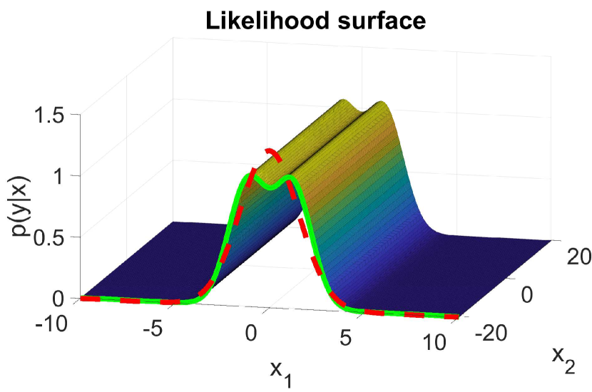
Figure 1: A likelihood surface with two components comprising $p(y|x)$ is shown, which can also be described in a reduced space shown in solid green. After component reduction, the likelihood function is approximated in the reduced space by the dashed red line, before being transformed back into the full state-space.

4.3 Algorithm overview

Algorithm 1 is provided to clarify the overall operation of the proposed solution to JMLS smoothing. We recommend implementing the proposed algorithm using square-root factors and log-weights for numerically stability. Additionally, for computational efficiency, components with zero weight do not need to be stored, and their statistics need not be calculated, this is often encountered when there is zero probability from transitioning from one model to another.

Algorithm 1 The Two-filter JMLS Smoother

1:The JMLS system parameters $\{\mathbf{A}_{k}(z_{k}),\mathbf{B}_{k}(z_{k}),\mathbf{Q}_{k}(z_{k}),\mathbf{C}_{k}(z_{k}),\mathbf{D}_{k}(z_{k}),\mathbf{R}_{k}(z_{k})\}_{z_{k}=1}^{m_{k}}$, defined model transition function $T_{k}$, measurement vector $y_{k}$ for timesteps $k=1,..,N$. The statistics for the prior $p(x_{1},z_{1})$ is also required.

2:for $k=1,\dots,N$ do

3:     Calculate the statistics of the forward filtered distribution $p(x_{k},z_{k}|y_{1:k})$ using Lemma 3.1.

4:     Perform KL reduction, detailed in Subsection 4.1, over the subsets of components in $p(x_{k},z_{k}|y_{1:k})$ with a common $z_{k}$ value.

5:     Calculate the statistics of the prediction distribution $p(x_{k+1},z_{k+1}|y_{1:k})$ using Lemma 3.1.

6:end for

7:Initialise the backwards information filter likelihood with $p(y_{N}|x_{N},z_{N})$ using Lemma 3.2.

8:for $k=N-1,\dots,1$ do

9:     Calculate the statistics of the backwards propagated likelihood $p(y_{k+1:N}|x_{k},z_{k})$ using Lemma 3.2.

10:     Using the method outlined in Subsection 4.2, perform likelihood reduction over the subsets of likelihood components in $p(y_{k+1:N}|x_{k},z_{k})$ with a common range-space and $z_{k}$ value.

11:     Calculate the statistics of the corrected likelihood $p(y_{k:N}|x_{k},z_{k})$ using Lemma 3.2.

12:end for

13:for $k=1,\dots,N-1$ do

14:     Generate the statistics for the hybrid smoothed distribution $p(x_{k},z_{k}|y_{1:N})$ using Lemma 3.3.

15:     (Optional) Perform KL reduction detailed in Subsection 4.1, over the subsets of components in $p(x_{k},z_{k}|y_{1:N})$ with a common $z_{k}$ value.

16:end for

5 Simulations

Here we provide the results from smoothing three different systems to demonstrate the effectiveness and versatility of the proposed solution.

5.1 Example 1 - Unimodal system

In this example we consider the unimodal linear Gaussian system

$$x_{k+1} =\mathbf{A}x_{k}+\mathbf{B}u_{k}+v_{k},$$ (43a)

$$y_{k} =\mathbf{C}x_{k}+\mathbf{D}u_{k}+e_{k},$$ (43b)

$$v_{k} \sim\mathcal{N}(v_{k}\mid{0},\mathbf{Q}),$$ (43c)

$$e_{k} \sim\mathcal{N}(e_{k}\mid{0},\mathbf{R}),$$ (43d)

which can be thought of as a single model JMLS with a model transition function of $T_{k}(z_{k+1}\mid z_{k})=1$. This system boycotts much of the difficulty with estimation of JMLS, as it does not require an exponentially growing number of components to be handled, and is included here for validation purposes of the smoothing equations.

The data for this example was generated using an input generated according to ${u}_{k}\sim\mathcal{N}(0,1)$ and the parameters

$$\mathbf{A} =0.9, \,\mathbf{B} =0.1, \,\mathbf{Q} =0.45,$$ (44)

$$\mathbf{C} =0.9, \,\mathbf{D} =0.05, \,\mathbf{R} =0.5.$$ (45)

Smoothing for this system was conducted for 13 timesteps using the proposed method and a RTS smoother to generate the ground truth data. Resulting smoothed distributions from both of these methods is shown in Figure 2 for comparison. As shown by this figure, both methods produce the same density, and are both exact for this system class.

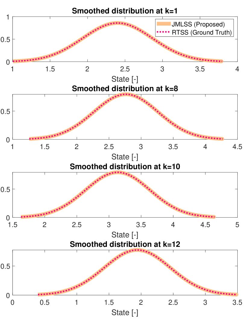
Figure 2: Generated smoothed distribution for Example 1, where the Rauch–Tung–Striebel smoother (RTSS) density (dotted red) is used as the ground truth, which can be compared to the JMLS smoother (JMLSS) density (solid orange).

5.2 Example 2 - A Jump Markov linear system

In this example we consider a JMLS system in the following form as used in [12, 16, 8, 3],

$$x_{k}=\mathbf{A}_{k}(z_{k})x_{k-1}+\mathbf{B}_{k}(z_{k})u_{k}+v_{k-1},$$ (46a)

$$y_{k}=\mathbf{C}_{k}(z_{k})x_{k}+\mathbf{D}_{k}(z_{k})u_{k}+e_{k},$$ (46b)

$$v_{k-1}\sim\mathcal{N}(v_{k-1}\mid{0},\mathbf{Q}_{k}(z_{k})),$$ (46c)

$$e_{k}\sim\mathcal{N}(e_{k}\mid{0},\mathbf{R}_{k}(z_{k})),$$ (46d)

this form differs from the system described in (1), as the above system uses a different time index for the switching parameter in the prediction step. To accommodate this, we modify the forward filter and proposed backward filter such that the model switches before the prediction step, and not after.

Since some of the alternate algorithms do not explain in detail how to perform likelihood reduction in the case of non-integrable likelihood functions, we use a single state system to circumvent this problem in order to compare their performance to the proposed method.

The parameters used for data generation and smoothing of this system were $u_{k}=1$ for all $k$ and

$$\mathbf{A}_{k}(1) =0.9,\ \mathbf{B}_{k}(1)=0.1,\ \mathbf{C}_{k}(1)=0.9,\ \mathbf{D}_{k}(1)=0.05,$$

$$\mathbf{A}_{k}(2) =0.9,\ \mathbf{B}_{k}(2)=0.12,\ \mathbf{C}_{k}(2)=0.85,\ \mathbf{D}_{k}(2)=0.05,$$

$$\mathbf{Q}_{k}(1) =0.45,\ \mathbf{R}_{k}(1)=0.5,$$

$$\mathbf{Q}_{k}(2) =0.01,\ \mathbf{R}_{k}(2)=1.5,\ \mathbf{T}=\begin{bmatrix}0.6&0.4\\ 0.4&0.6\end{bmatrix},$$ (47)

where $T_{k}(i|j)=\mathbf{T}_{i,j}$.

The system was simulated for $N=15$ time steps to produce input-output data. A range of smoothers were run on this data including the proposed method (abbreviated as JMLSS) and other smothers including the IMM, GPB2, and aSLDS EC smoother. A particle smoother (PS) solution was also implemented to provide a ground truth estimate, however it took orders of magnitude longer to run. This experiment repeated 250 times with different datasets, where the distributions were used to calculate a mean KL divergence error over each timeseries for each of the methods, which in turn was used to generate the boxplot in Figure 3. Figure 3 shows that the proposed methods outperformed the alterative approaches in each of these 250 runs, often by an order of magnitude. Additionally Figure 4 shows distributions from each of the smoothers during one of these runs.

It is important to also compare the computation time for these methods, since it can be argued that the approximation error of the JMLS smoother presented in this paper can always be reduced by allowing more components. Table 1 records the computation time for each method (all methods were implemented in native Matlab code). It may be concluded that the computation time associated with the JMLSS is an order of magnitude more than the fastest method, but around two orders of magnitude better in terms of accuracy.

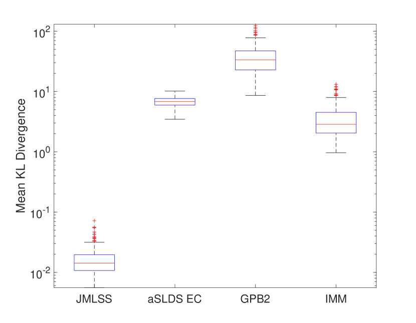
Figure 3: Boxplot [21] of KL divergence over 250 random smoothed datasets for Example 2 using the proposed JMLS smoother (JMLSS), and other alternative IMM, GPB2, and aSLDS EC smoothers.

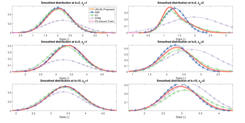
Figure 4: Generated smoothed distributions for the JMLS system from Example 2, where the Particle Smoother (PS) density (dotted red) is used as the ground truth, and the distribution from the proposed JMLS smoother (JMLSS) (solid orange) is compared against the distributions from the alternate interacting multiple model (IMM) (blue with triangles), expectation correction (aSLDS EC) (green with circles), generalised pseudo-Bayesian (GPB2) (light purple with squares) smoothers.

Table 1: Computation time (seconds) for Example 2.

PS	JMLSS	aSLSDS EC	GPB2	IMM
16598	0.39	0.45	0.02	0.04

5.3 Example 3 - Dynamic JMLS system

In this example we consider a two-state problem, which takes full advantage of the proposed likelihood reduction strategy, as it is a multi-state problem which presents with non-integrable likelihood components in the BIF. The example considers the dynamical model of a mass-spring-damper (MSD) system with a position sensor

$$m\ddot{x}(t)+b\dot{x}(t)+kx(t) =F(t),$$ (48a)

$$y(t) =x(t),$$ (48b)

where $x(t)$ is the mass position, $F(t)$ is the applied external force, $m$ is the system mass, $b$ is the damping coefficient and $k$ is the spring constant. We further assume that the system can use one of two available sets of parameters, indicated by a superscript, at any timestep,

$$m^{1}=8[\textrm{kg}],\,b^{1}=12[\textrm{Ns/m}],\,k^{1}=10[\textrm{N/m}],$$

$$m^{2}=8[\textrm{kg}],\,b^{2}=0[\textrm{Ns/m}],\,k^{2}=0[\textrm{N/m}].$$ (49)

The second parameter set represents a possible fault scenario, where the the spring and damper have become disconnected from the mass, the transition matrix for this example was chosen to reflect a 1% chance of permanent failure

$$\mathbf{T}_{i,j}=\begin{bmatrix}0.99&0\\ 0.01&1\end{bmatrix}.$$ (50)

Using an approach similar to that in [18, 26], the models were discretised and converted into the model class (1) using a sample rate of 100Hz and simulated ADC sample time of $0.1$ms. The system was assumed to be driven by $F[k]=2000\sin(k/(20\pi))$, then smoothed using the proposed method and a particle smoother (PS) to provide a ground truth. As other alternative smoothers without modification do not support the system form (1) required for this discretisation, they do not appear in this experiment.

The resulting marginalised distributions from this experiment are shown in Figure 5. Note that the system could easily be smoothed for a larger number of timesteps using the proposed computationally inexpensive closed-form solution, but was set to $N=10$ due to the large computational expense of the particle smoother. It is also possible to increase number of models to accommodate a variety of other fault scenarios, such as sensor failure.

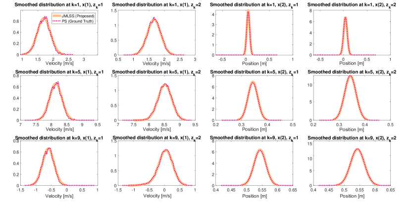
Figure 5: Generated smoothed distributions for the dynamic JMLS system from Example 3, where the particle smoother (PS) distribution (dotted red) is used as the ground truth, and compared against the distribution from the proposed JMLS smoother (JMLSS) (solid orange).

6 Conclusion

We have developed a new smoothing algorithm for jump-Markov-linear-systems using a two-filter approach. This contribution has two components. Firstly, we have developed an algorithm that implements the two-filter smoothing formulas exactly, therefore relaxing assumptions imposed by competing methods. Secondly, we have developed an approximation method that allows likelihood reduction that, contrary to existing methods, does not require likelihoods to have a Gaussian form in order to perform merging. The implication is that the new method presents the user with a mechanism to choose between computational cost and accuracy, making it suitable for both real-time and post processing applications. This accuracy-computational cost tradeoff was demonstrated by way of example.

Compared to alternatives, the proposed approach is very well suited to applications where likelihood modes in the BIF are non-integrable over $x_{k}$. This can be encountered for a number of reasons, and is a common occurrence in the first few iterations of the BIF. This property allows the JMLS estimator to handle models with only partial observability of the system state, which is useful for applications in fault diagnosis.

Appendix A Forward and backward filtering Lemmata

Recall the definition of $\xi\triangleq\{x_{k},z_{k}\}$ from Section 2, and recall that for an integrable function $f$,

$$\int f(\xi_{k})p(\xi_{k})d\xi_{k}\triangleq\sum_{z_{k}=1}^{m_{k}}\int f(x_{k},z_{k})p(x_{k},z_{k})dx_{k}.$$ (51)

A.1 Proof of Lemma 3.2

Begin by constructing

$$p (y_{k+1:N}|\xi_{k})$$

$$= \int p(y_{k+1:N}|\xi_{k+1})p(\xi_{k+1}|\xi_{k})\,d\xi_{k+1}$$

$$= \int\sum_{i=1}^{M^{\text{c}}_{k+1}}\mathcal{L}(x_{k+1}|\bar{r}^{i}_{k+1}(z_{k+1}),\bar{s}^{i}_{k+1}(z_{k+1}),\bar{\mathbf{L}}^{i}_{k+1}(z_{k+1}))$$

$$\cdot T(z_{k+1}|z_{k})\mathcal{N}(x_{k+1}|\mathbf{A}_{k}(z_{k})x_{k}+b_{k}(z_{k}),\mathbf{Q}_{k}(z_{k}))\,d\xi_{k+1}$$

$$= \sum_{z_{k+1}=1}^{m_{k+1}}\int\sum_{i=1}^{M^{\text{c}}_{k+1}}\mathcal{L}(x_{k+1}|\bar{r}^{i}_{k+1}(z_{k+1}),\bar{s}^{i}_{k+1}(z_{k+1}),\bar{\mathbf{L}}^{i}_{k+1}(z_{k+1}))$$

$$\cdot T(z_{k+1}|z_{k})\mathcal{N}(x_{k+1}|\mathbf{A}_{k}(z_{k})x_{k}+b_{k}(z_{k}),\mathbf{Q}_{k}(z_{k}))\,d\xi_{k+1}$$

$$= \sum_{z_{k+1}=1}^{m_{k+1}}\sum_{i=1}^{M^{\text{c}}_{k+1}}T(z_{k+1}|z_{k})$$

$$\cdot\int\mathcal{L}(x_{k+1}|\bar{r}^{i}_{k+1}(z_{k+1}),\bar{s}^{i}_{k+1}(z_{k+1}),\bar{\mathbf{L}}^{i}_{k+1}(z_{k+1}))$$

$$\cdot\mathcal{N}(x_{k+1}|\mathbf{A}_{k}(z_{k})x_{k}+b_{k}(z_{k}),\mathbf{Q}_{k}(z_{k}))\,d\xi_{k+1}.$$ (52)

Applying Lemma B.1 yields

$$= \sum_{z_{k+1}=1}^{m_{k+1}}\sum_{i=1}^{M^{\text{c}}_{k+1}}T(z_{k+1}|z_{k})$$

$$\cdot\mathcal{L}(x_{k}|\tilde{r}^{i}_{k}(z_{k},z_{k+1}),{s}^{i}_{k}(z_{k},z_{k+1}),\mathbf{L}^{i}_{k}(z_{k},z_{k+1})).$$ (53)

Absorbing the transition probability into the information scalar yields

$$= \sum_{z_{k+1}=1}^{m_{k+1}}\sum_{i=1}^{M^{\text{c}}_{k+1}}\mathcal{L}(x_{k}|{r}^{i}_{k}(z_{k},z_{k+1}),{s}^{i}_{k}(z_{k},z_{k+1}),\mathbf{L}^{i}_{k}(z_{k},z_{k+1})),$$ (54)

where

$${r}^{i}_{k}(z_{k},z_{k+1})=\tilde{r}^{i}_{k}(z_{k},z_{k+1})-2\ln(T(z_{k+1}|z_{k})).$$ (55)

Finally, the double sum indices $\{z_{k+1},i\}$ can be collapsed into single index $j$,

$$= \sum_{j=1}^{M^{\text{b}}_{k}}\mathcal{L}(x_{k}|r^{j}_{k}(z_{k}),s^{j}_{k}(z_{k}),\mathbf{L}^{j}_{k}(z_{k})),$$ (56)

where ${M^{\text{b}}_{k}}=m_{k+1}{M^{\text{c}}_{k+1}}$.

The proof for the expressions in (23) and (24) is provided below

$$p (y_{k+1:N}|\xi_{k+1})$$

$$= p(y_{k+2:N}|\xi_{k+1})p(y_{k+1}|\xi_{k+1})$$

$$= \sum_{i=1}^{{M^{\text{b}}_{k+1}}}\mathcal{L}(x_{k+1}|r_{k+1}^{i}(z_{k+1}),s_{k+1}^{i}(z_{k+1}),\mathbf{L}_{k+1}^{i}(z_{k+1}))$$

$$\cdot\mathcal{N}(y_{k+1}|\mathbf{C}_{k+1}(z_{k+1})x_{k+1}+d_{k+1}(z_{k+1}),\mathbf{R}_{k+1}(z_{k+1})).$$ (57)

Using Lemma B.2,

$$= \sum_{i=1}^{{M^{\text{b}}_{k+1}}}\mathcal{L}(x_{k+1}|\bar{r}_{k+1}^{i}(z_{k+1}),\bar{s}_{k+1}^{i}(z_{k+1}),\bar{\mathbf{L}}_{k+1}^{i}(z_{k+1})),$$ (58)

finally let ${M^{\text{c}}_{k+1}}={M^{\text{b}}_{k+1}}$,

$$= \sum_{i=1}^{{M^{\text{c}}_{k+1}}}\mathcal{L}(x_{k+1}|\bar{r}_{k+1}^{i}(z_{k+1}),\bar{s}_{k+1}^{i}(z_{k+1}),\bar{\mathbf{L}}_{k+1}^{i}(z_{k+1})).$$ (59)

∎

A.2 Proof of Lemma 3.3

Begin by constructing

$$p (y_{k+1:N}|\xi_{k})p(\xi_{k}|y_{1:k})$$

$$= \sum_{\ell=1}^{{M^{\text{b}}_{k}}}\mathcal{L}(x_{k}|\bar{r}_{k}^{\ell}(z_{k}),\bar{s}_{k}^{\ell}(z_{k}),\bar{\mathbf{L}}_{k}^{\ell}(z_{k}))$$

$$\cdot\sum_{i=1}^{M^{\text{f}}_{k}}w_{k|k}^{i}(z_{k})\mathcal{N}(x_{k}|\mu_{k|k}^{i}(z_{k}),\mathbf{P}_{k|k}^{i}(z_{k})),$$ (60)

before using Lemma B.3 to yield

$$= \sum_{\ell=1}^{{M^{\text{b}}_{k}}}\sum_{i=1}^{M^{\text{f}}_{k}}\tilde{w}_{k|N}^{(i,\ell)}(z_{k})\mathcal{N}(x_{k}|\mu_{k|N}^{(i,\ell)}(z_{k}),\mathbf{P}_{k|N}^{(i,\ell)}(z_{k})).$$ (61)

Collapse double sum indices $\{i,\ell\}$ into single sum $j$

$$= \sum_{j=1}^{{M^{\text{s}}_{k}}}\tilde{w}_{k|N}^{j}(z_{k})\mathcal{N}(x_{k}|\mu_{k|N}^{j}(z_{k}),\mathbf{P}_{k|N}^{j}(z_{k})),$$ (62)

where ${M^{\text{s}}_{k}}={M^{\text{f}}_{k}}{M^{\text{b}}_{k}}$. Now concentrating on the smoothed distribution

$$p(\xi_{k}|y_{1:N})= \frac{p(y_{k+1:N}|\xi_{k})p(\xi_{k}|y_{1:k})}{p(y_{k+1:N}|y_{1:k})}$$

$$= \frac{p(y_{k+1:N}|\xi_{k})p(\xi_{k}|y_{1:k})}{\int p(y_{k+1:N}|\xi_{k})p(\xi_{k}|y_{1:k})\,d\xi_{k}}$$

$$= \frac{p(y_{k+1:N}|\xi_{k})p(\xi_{k}|y_{1:k})}{\sum_{z_{k}=1}^{m_{k}}\int p(y_{k+1:N}|\xi_{k})p(\xi_{k}|y_{1:k})\,dx_{k}},$$ (63)

now substituting (62) yields

$$= \frac{\sum_{j=1}^{{M^{\text{s}}_{k}}}\tilde{w}_{k|N}^{j}(z_{k})\mathcal{N}(x_{k}|\mu_{k|N}^{j}(z_{k}),\mathbf{P}_{k|N}^{j}(z_{k}))}{\sum_{z_{k}=1}^{m_{k}}\int\sum_{j=1}^{{M^{\text{s}}_{k}}}\tilde{w}_{k|N}^{j}(z_{k})\mathcal{N}(x_{k}|\mu_{k|N}^{j}(z_{k}),\mathbf{P}_{k|N}^{j}(z_{k}))\,dx_{k}}$$

$$= \frac{\sum_{j=1}^{{M^{\text{s}}_{k}}}\tilde{w}_{k|N}^{j}(z_{k})\mathcal{N}(x_{k}|\mu_{k|N}^{j}(z_{k}),\mathbf{P}_{k|N}^{j}(z_{k}))}{\sum_{z_{k}=1}^{m_{k}}\sum_{j=1}^{{M^{\text{s}}_{k}}}\tilde{w}_{k|N}^{j}(z_{k})}$$

$$= \sum_{j=1}^{{M^{\text{s}}_{k}}}{w}_{k|N}^{j}(z_{k})\mathcal{N}(x_{k}|\mu_{k|N}^{j}(z_{k}),\mathbf{P}_{k|N}^{j}(z_{k})),$$ (64)

where

$${w}_{k|N}^{j}(z_{k})=\frac{\tilde{w}_{k|N}^{j}(z_{k})}{\sum_{z_{k}=1}^{m_{k}}\sum_{j=1}^{{M^{\text{s}}_{k}}}\tilde{w}_{k|N}^{j}(z_{k})}.$$ (65)

∎

Appendix B Additional Lemata

Lemma B.1.

Let ${\bar{\mathbf{L}}}$, $\bar{s}$, and $\bar{r}$ be the information matrix, information vector and information scalar respectively, the sufficient statistics for a likelihood component in the BIF. Then given a Gaussian state-transition distribution parameterised by $\mathbf{A}$, and $b$, with an invertible process covariance $\mathbf{Q}$, then the statistics for the BIF likelihood can be backwards propagated as

$$\mathcal{L}(x|r,s,\mathbf{L})$$

$$=\int\mathcal{N}(\hat{x}|\mathbf{A}x+b,\mathbf{Q})\mathcal{L}(\hat{x}|\bar{r},\bar{s},\bar{\mathbf{L}})\,d\hat{x},$$ (66)

where ${\mathbf{L}}$, ${s}$, and ${r}$ are the updated statistics. These statistics can be calculated using

$$\mathbf{L} =\mathbf{A}^{T}\boldsymbol{\Phi}\mathbf{A},$$ (67)

$$s =\mathbf{A}^{T}(\boldsymbol{\Phi}b+\boldsymbol{\Gamma}^{T}\bar{s}),$$ (68)

$$r =\bar{r}-\ln{|\boldsymbol{\Gamma}|}+\begin{bmatrix}\bar{s}\\ b\end{bmatrix}^{T}\begin{bmatrix}\boldsymbol{\Psi}&\boldsymbol{\Gamma}\\ \boldsymbol{\Gamma}^{T}&\boldsymbol{\Phi}\end{bmatrix}\begin{bmatrix}\bar{s}\\ b\end{bmatrix},$$ (69)

$$\boldsymbol{\Gamma} =\mathbf{I}-\mathbf{Q}\boldsymbol{\Phi},$$ (70)

$$\boldsymbol{\Psi} =\mathbf{Q}\boldsymbol{\Phi}\mathbf{Q}-\mathbf{Q},$$ (71)

$$\boldsymbol{\Phi} =\Bigl{(}\mathbf{I}+\bar{\mathbf{L}}\mathbf{Q}\Bigr{)}^{-1}\bar{\mathbf{L}}.$$ (72)

Proof.

Begin with the Gaussian state-transition distribution

$$\mathcal{N} (\hat{x}|\mathbf{A}x+b,\mathbf{Q})$$

$$= e^{-0.5(x^{p}-\hat{x})^{T}\mathbf{Q}^{-1}(x^{p}-\hat{x})-0.5\ln|2\pi\mathbf{Q}|}$$

$$= e^{-0.5(\hat{x}^{T}\mathbf{Q}^{-1}\hat{x}-2\hat{x}^{T}\mathbf{Q}^{-1}x^{p}+(x^{p})^{T}\mathbf{Q}^{-1}x^{p}+\ln|2\pi\mathbf{Q}|)},$$ (73)

where $x^{p}=\mathbf{A}x+b.$ Therefore

$$\int \mathcal{N}(\hat{x}|\mathbf{A}x+b,\mathbf{Q})\mathcal{L}(\hat{x}|\bar{r},\bar{s},\bar{\mathbf{L}})\,d\hat{x}$$

$$=\int\mathcal{N}(\hat{x}|\mathbf{A}x+b,\mathbf{Q})e^{-0.5(\hat{x}^{T}\bar{\mathbf{L}}\hat{x}+2\hat{x}^{T}\bar{s}+\bar{r})}\,d\hat{x}$$

$$=\int e^{-0.5(\hat{x}^{T}\hat{\mathbf{L}}\hat{x}+2\hat{x}^{T}\hat{s}+\hat{r})}\,d\hat{x}$$

$$=\int e^{-0.5\hat{r}}e^{-0.5(\hat{x}^{T}\hat{\mathbf{L}}\hat{x}+2\hat{x}^{T}\hat{s})}\,d\hat{x},$$ (74)

where,

$$\hat{\mathbf{L}} =\bar{\mathbf{L}}+\mathbf{Q}^{-1},$$ (75a)

$$\hat{s} =\bar{s}-\mathbf{Q}^{-1}x^{p},$$ (75b)

$$\hat{r} =\bar{r}+(x^{p})^{T}\mathbf{Q}^{-1}x^{p}+\ln|2\pi\mathbf{Q}|.$$ (75c)

Using the normalising constant for a Gaussian we can derive an expression to perform the required integration,

$$|2\pi\mathbf{P}|^{0.5}=\int e^{-0.5(x^{T}\mathbf{P}^{-1}x-2x^{T}\mathbf{P}^{-1}\mu+\mu^{T}\mathbf{P}^{-1}\mu)}\,dx,$$ (76)

$$\therefore\int e^{-0.5(x^{T}\mathbf{P}^{-1}x-2x^{T}\mathbf{P}^{-1}\mu)}\,dx=|2\pi\mathbf{P}|^{0.5}e^{0.5\mu^{T}\mathbf{P}^{-1}\mu}.$$ (77)

Substituting in the relationship to information form,
$\mathbf{P}^{-1}=\hat{\mathbf{L}}$, $\mu=-\hat{\mathbf{L}}^{-1}\hat{s}$, and noting that $\hat{\mathbf{L}}^{T}=\hat{\mathbf{L}}$ yields

$$\int e^{-0.5(x^{T}\hat{\mathbf{L}}x+2x^{T}\hat{\mathbf{L}}\hat{\mathbf{L}}^{-1}\hat{s})}\,dx=|2\pi\hat{\mathbf{L}}^{-1}|^{0.5}e^{0.5\hat{s}^{T}\hat{\mathbf{L}}^{-1}\hat{\mathbf{L}}\hat{\mathbf{L}}^{-1}\hat{s}},$$ (78)

$$\int e^{-0.5(x^{T}\hat{\mathbf{L}}x+2x^{T}\hat{s})}\,dx=|2\pi\hat{\mathbf{L}}^{-1}|^{0.5}e^{0.5\hat{s}^{T}\hat{\mathbf{L}}^{-1}\hat{s}}.$$ (79)

We can now use this result to integrate (74) over $\hat{x}$,

$$\int \mathcal{N}(\hat{x}|\mathbf{A}x+b,\mathbf{Q})\mathcal{L}(\hat{x}|\bar{r},\bar{s},\bar{\mathbf{L}})\,d\hat{x}$$

$$=e^{-0.5\hat{r}}\int e^{-0.5(\hat{x}^{T}\hat{\mathbf{L}}\hat{x}+2\hat{x}^{T}\hat{s})}\,d\hat{x}$$

$$=e^{-0.5\hat{r}}|2\pi\hat{\mathbf{L}}^{-1}|^{0.5}e^{0.5\hat{s}^{T}\hat{\mathbf{L}}^{-1}\hat{s}}$$

$$=e^{-0.5(\hat{r}-\hat{s}^{T}\hat{\mathbf{L}}^{-1}\hat{s}-\ln|2\pi\hat{\mathbf{L}}^{-1}|)}.$$ (80)

Back substituting (75b) and (75c)

$$= \exp\bigg{[}-0.5\bigg{(}\bar{r}+(x^{p})^{T}\mathbf{Q}^{-1}x^{p}+\ln|2\pi\mathbf{Q}|$$

$$-(\bar{s}-\mathbf{Q}^{-1}x^{p})^{T}\hat{\mathbf{L}}^{-1}(\bar{s}-\mathbf{Q}^{-1}x^{p})-\ln|2\pi\hat{\mathbf{L}}^{-1}|\bigg{)}\bigg{]}$$

$$= \exp\bigg{[}-0.5\bigg{(}\bar{r}+\ln|2\pi\mathbf{Q}|-\ln|2\pi\hat{\mathbf{L}}^{-1}|+(x^{p})^{T}\mathbf{Q}^{-1}x^{p}$$

$$-\bar{s}^{T}\hat{\mathbf{L}}^{-1}\bar{s}+2\bar{s}^{T}\hat{\mathbf{L}}^{-1}\mathbf{Q}^{-1}x^{p}-(x^{p})^{T}\mathbf{Q}^{-1}\hat{\mathbf{L}}^{-1}\mathbf{Q}^{-1}x^{p}\bigg{)}\bigg{]}$$

$$= \exp\bigg{[}-0.5\bigg{(}\bar{r}+\ln|2\pi\mathbf{Q}|-\ln|2\pi\hat{\mathbf{L}}^{-1}|-\bar{s}^{T}\hat{\mathbf{L}}^{-1}\bar{s}$$

$$+(x^{p})^{T}(\mathbf{Q}^{-1}-\mathbf{Q}^{-1}\hat{\mathbf{L}}^{-1}\mathbf{Q}^{-1})x^{p}+2\bar{s}^{T}\hat{\mathbf{L}}^{-1}\mathbf{Q}^{-1}x^{p}\bigg{)}\bigg{]}$$

$$= \exp\bigg{[}-0.5\bigg{(}\bar{r}+\ln|\mathbf{Q}|-\ln|\hat{\mathbf{L}}^{-1}|-\bar{s}^{T}\hat{\mathbf{L}}^{-1}\bar{s}$$

$$+(x^{p})^{T}(\mathbf{Q}^{-1}-\mathbf{Q}^{-1}\hat{\mathbf{L}}^{-1}\mathbf{Q}^{-1})x^{p}+2\bar{s}^{T}\hat{\mathbf{L}}^{-1}\mathbf{Q}^{-1}x^{p}\bigg{)}\bigg{]}.$$ (81)

Using the Woodbury matrix identity:
$A^{-1}-(UCV+A)^{-1}=A^{-1}U(C^{-1}+VA^{-1}U)^{-1}VA^{-1}$ with $U=C=\mathbf{I}$, $V=\bar{\mathbf{L}}$, and $A=\mathbf{Q}^{-1}$ yields the useful relations

$$\mathbf{Q}-(\underbrace{\bar{\mathbf{L}}+\mathbf{Q}^{-1}}_{\hat{\mathbf{L}}})^{-1}=\mathbf{Q}\underbrace{(\mathbf{I}+\bar{\mathbf{L}}\mathbf{Q})^{-1}\bar{\mathbf{L}}}_{\boldsymbol{\Phi}}\mathbf{Q},$$ (82)

and

$$\therefore\mathbf{Q}^{-1}-\mathbf{Q}^{-1}(\underbrace{\bar{\mathbf{L}}+\mathbf{Q}^{-1}}_{\hat{\mathbf{L}}})^{-1}\mathbf{Q}^{-1}=(\mathbf{I}+\bar{\mathbf{L}}\mathbf{Q})^{-1}\bar{\mathbf{L}}=\boldsymbol{\Phi}.$$ (83)

Substituting (83) into (B)

$$= \exp\bigg{[}-0.5\bigg{(}\bar{r}+\ln|\mathbf{Q}|-\ln|\hat{\mathbf{L}}^{-1}|-\bar{s}^{T}\hat{\mathbf{L}}^{-1}\bar{s}$$

$$+(x^{p})^{T}\boldsymbol{\Phi}x^{p}+2\bar{s}^{T}\hat{\mathbf{L}}^{-1}\mathbf{Q}^{-1}x^{p}\bigg{)}\bigg{]}.$$ (84)

From (82) $\mathbf{Q}-\hat{\mathbf{L}}^{-1}=\mathbf{Q}\boldsymbol{\Phi}\mathbf{Q}$, $\therefore\hat{\mathbf{L}}=(\mathbf{Q}-\mathbf{Q}\boldsymbol{\Phi}\mathbf{Q})^{-1}$, and therefore

$$\ln|\mathbf{Q}|-\ln|\hat{\mathbf{L}}^{-1}|=\ln|\mathbf{Q}\hat{\mathbf{L}}|$$

$$=\ln|\mathbf{Q}(\mathbf{Q}-\mathbf{Q}\boldsymbol{\Phi}\mathbf{Q})^{-1}|=\ln|(\mathbf{I}-\mathbf{Q}\boldsymbol{\Phi})^{-1}|$$

$$=-\ln|\boldsymbol{\Gamma}|,\text{where }\boldsymbol{\Gamma}=(\mathbf{I}-\mathbf{Q}\boldsymbol{\Phi}),$$ (85)

which can be substituted into (B) to yield

$$= \exp\bigg{[}-0.5\bigg{(}\bar{r}-\ln|\boldsymbol{\Gamma}|-\bar{s}^{T}\hat{\mathbf{L}}^{-1}\bar{s}+(x^{p})^{T}\boldsymbol{\Phi}x^{p}$$

$$+2\bar{s}^{T}\hat{\mathbf{L}}^{-1}\mathbf{Q}^{-1}x^{p}\bigg{)}\bigg{]}.$$ (86)

By rearrangement of (82)

$$\hat{\mathbf{L}}^{-1}\mathbf{Q}^{-1}=(\mathbf{Q}-\mathbf{Q}\boldsymbol{\Phi}\mathbf{Q})\mathbf{Q}^{-1}=\mathbf{I}-\mathbf{Q}\boldsymbol{\Phi}=\boldsymbol{\Gamma},$$ (87)

and

$$\hat{\mathbf{L}}^{-1}=\mathbf{Q}-\mathbf{Q}\boldsymbol{\Phi}\mathbf{Q}=-\boldsymbol{\Psi}.$$ (88)

Substituting (87) and (88) into (B) yields

$$= \exp\bigg{[}-0.5\bigg{(}\bar{r}-\ln|\boldsymbol{\Gamma}|+\bar{s}^{T}\boldsymbol{\Psi}\bar{s} +(x^{p})^{T}\boldsymbol{\Phi}x^{p}+2\bar{s}^{T}\boldsymbol{\Gamma}x^{p}\bigg{)}\bigg{]}.$$ (89)

Finally, by back substituting $x^{p}=\mathbf{A}x+b$,

$$= \exp\bigg{[}-0.5\bigg{(}\bar{r}-\ln|\boldsymbol{\Gamma}|+\bar{s}^{T}\boldsymbol{\Psi}\bar{s}$$

$$+(\mathbf{A}x+b)^{T}\boldsymbol{\Phi}(\mathbf{A}x+b)+2\bar{s}^{T}\boldsymbol{\Gamma}(\mathbf{A}x+b)\bigg{)}\bigg{]}$$ (90)

$$= \exp\bigg{[}-0.5\bigg{(}\bar{r}-\ln|\boldsymbol{\Gamma}|+\bar{s}^{T}\boldsymbol{\Psi}\bar{s}$$

$$+x^{T}\mathbf{A}^{T}\boldsymbol{\Phi}\mathbf{A}x+2b^{T}\boldsymbol{\Phi}\mathbf{A}x+b^{T}\boldsymbol{\Phi}b+2\bar{s}^{T}\boldsymbol{\Gamma}\mathbf{A}x+2\bar{s}^{T}\boldsymbol{\Gamma}b\bigg{)}\bigg{]}$$ (91)

$$= \exp\bigg{[}-0.5\bigg{(}\bar{r}-\ln|\boldsymbol{\Gamma}|+\bar{s}^{T}\boldsymbol{\Psi}\bar{s}+\bar{s}^{T}\boldsymbol{\Gamma}b+b^{T}\boldsymbol{\Gamma}^{T}\bar{s}+b^{T}\boldsymbol{\Phi}b$$

$$+x^{T}\mathbf{A}^{T}\boldsymbol{\Phi}\mathbf{A}x+2(b^{T}\boldsymbol{\Phi}\mathbf{A}+\bar{s}^{T}\boldsymbol{\Gamma}\mathbf{A})x\bigg{)}\bigg{]}$$ (92)

$$= \exp\bigg{[}-0.5\bigg{(}x^{T}\underbrace{\mathbf{A}^{T}\boldsymbol{\Phi}\mathbf{A}}_{\mathbf{L}}x+2x^{T}\underbrace{\mathbf{A}^{T}(\boldsymbol{\Phi}b+\boldsymbol{\Gamma}^{T}\bar{s})}_{s}$$

$$+\underbrace{\bar{r}-\ln|\boldsymbol{\Gamma}|+\begin{bmatrix}\bar{s}\\ b\end{bmatrix}^{T}\begin{bmatrix}\boldsymbol{\Psi}&\boldsymbol{\Gamma}\\ \boldsymbol{\Gamma}^{T}&\boldsymbol{\Phi}\end{bmatrix}\begin{bmatrix}\bar{s}\\ b\end{bmatrix}}_{r}\bigg{)}\bigg{]},$$

$$= \mathcal{L}(x|r,s,\mathbf{L}).$$ (93)

Note that unlike $\boldsymbol{\Psi}$ and $\boldsymbol{\Phi}$, $\boldsymbol{\Gamma}$ is not necessarily symmetric. ∎

Lemma B.2.

Let ${\mathbf{L}}$, ${s}$, and ${r}$ be the information matrix, information vector and information scalar respectively, the sufficient statistics for a likelihood component in the BIF. Then given a measurement $y$, and the parameters for the output equation $\mathbf{C}$, and $d$, with an invertible measurement covariance $\mathbf{R}$, then the statistics for the BIF likelihood component can be corrected by the a Gaussian likelihood as

$$\mathcal{L}(x|\bar{r},\bar{s},\bar{\mathbf{L}})=\mathcal{N}(y|\mathbf{C}x+d,\mathbf{R})\mathcal{L}(x|{r},{s},{\mathbf{L}}),$$ (94)

where $\bar{\mathbf{L}}$, $\bar{s}$, and $\bar{r}$ are the corrected statistics. These statistics can be calculated using

$$\bar{\mathbf{L}} =\mathbf{L}+\mathbf{C}^{T}\mathbf{R}^{-1}\mathbf{C},$$ (95)

$$\bar{s} =s+\mathbf{C}^{T}\mathbf{R}^{-1}\zeta,$$ (96)

$$\bar{r} =r+\zeta^{T}\mathbf{R}^{-1}\zeta+\ln|2\pi\mathbf{R}|,$$ (97)

$$\zeta =d-y.$$ (98)

Proof.

Begin with the linear Gaussian measurement likelihood

$$\mathcal{N}( y|\mathbf{C}x+d,\mathbf{R})$$

$$= e^{-0.5(x^{T}\mathbf{C}^{T}+\zeta^{T})\mathbf{R}^{-1}(\mathbf{C}x+\zeta)-0.5\ln|2\pi\mathbf{R}|}$$

$$= \exp[-0.5(x^{T}\mathbf{C}^{T}\mathbf{R}^{-1}\mathbf{C}x+2x^{T}\mathbf{C}^{T}\mathbf{R}^{-1}\zeta$$

$$+\zeta^{T}\mathbf{R}^{-1}\zeta+\ln|2\pi\mathbf{R}|)].$$ (99)

Therefore

$$\mathcal{N} (y|\mathbf{C}x+d,\mathbf{R})\mathcal{L}(x|{r},{s},{\mathbf{L}})$$

$$= \mathcal{N}(y|\mathbf{C}x+d,\mathbf{R})e^{-0.5(x^{T}\mathbf{L}x+2x^{T}s+r)}$$

$$= \exp[-0.5(x^{T}(\mathbf{L}+\mathbf{C}^{T}\mathbf{R}^{-1}\mathbf{C})x+2x^{T}(s+\mathbf{C}^{T}\mathbf{R}^{-1}\zeta)$$

$$+r+\zeta^{T}\mathbf{R}^{-1}\zeta+\ln|2\pi\mathbf{R}|)]$$

$$= e^{-0.5(x^{T}\bar{\mathbf{L}}x+2x^{T}\bar{s}+\bar{r})}=\mathcal{L}(x|\bar{r},\bar{s},\bar{\mathbf{L}}).$$ (100)

∎

Lemma B.3.

Let ${\bar{\mathbf{L}}}$, $\bar{s}$, and $\bar{r}$ be the information matrix, information vector and information scalar respectively, the sufficient statistics for a likelihood component in the BIF. Additionally, let $\mathbf{P}$, $\mu$, and $w$ be the covariance matrix, mean and weight of a Gaussian mode. Then the statistics of the combined smoothed component $\{\bar{\mathbf{P}},\bar{\mu},\bar{w}\}$ can be computed as

$$\bar{w}\mathcal{N}(x|\bar{\mu},\bar{\mathbf{P}})=w\mathcal{N}(x|\mu,\mathbf{P})\mathcal{L}(x|r,s,\mathbf{L}),$$ (101)

where

$$\bar{\mathbf{P}} =(\mathbf{P}^{-1}+\mathbf{L})^{-1},$$ (102a)

$$\bar{\mu} =\bar{\mathbf{P}}(\mathbf{P}^{-1}\mu-s),$$ (102b)

$$\bar{w} =\frac{w{|2\pi\bar{\mathbf{P}}|}^{\frac{1}{2}}e^{\frac{1}{2}\beta}}{{|2\pi\mathbf{P}|}^{\frac{1}{2}}},$$ (102c)

$$\beta =\bar{\mu}^{T}\bar{\mathbf{P}}^{-1}\bar{\mu}-\mu^{T}\mathbf{P}^{-1}\mu-r$$ (102d)

Proof.

$$w \mathcal{N}(x|\mu,\mathbf{P})\mathcal{L}(x|r,s,\mathbf{L})$$

$$=\frac{w}{{|2\pi\mathbf{P}|}^{\frac{1}{2}}}e^{-\frac{1}{2}(x^{T}\mathbf{P}^{-1}x-2x^{T}\mathbf{P}^{-1}\mu+\mu^{T}\mathbf{P}^{-1}\mu)}e^{-\frac{1}{2}(x^{T}\mathbf{L}x+2x^{T}s+r)}$$

$$=\frac{we^{-\frac{1}{2}(\mu^{T}\mathbf{P}^{-1}\mu+r)}}{{|2\pi\mathbf{P}|}^{\frac{1}{2}}}e^{-\frac{1}{2}\left(x^{T}(\mathbf{P}^{-1}+\mathbf{L})x-2x^{T}(\mathbf{P}^{-1}\mu-s)\right)}$$ (103)

let $\bar{\mathbf{P}}^{-1}=\mathbf{P}^{-1}+\mathbf{L}$, and $\bar{\mu}=\bar{\mathbf{P}}(\mathbf{P}^{-1}\mu-s)$

$$= \frac{we^{-\frac{1}{2}(\mu^{T}\mathbf{P}^{-1}\mu+r)}}{{|2\pi\mathbf{P}|}^{\frac{1}{2}}}e^{-\frac{1}{2}(x^{T}\bar{\mathbf{P}}^{-1}x-2x^{T}\bar{\mathbf{P}}^{-1}\bar{\mu})}$$

$$= \frac{w{|2\pi\bar{\mathbf{P}}|}^{\frac{1}{2}}e^{-\frac{1}{2}(\mu^{T}\mathbf{P}^{-1}\mu+r-\bar{\mu}^{T}\bar{\mathbf{P}}^{-1}\bar{\mu})}}{{|2\pi\mathbf{P}|}^{\frac{1}{2}}{|2\pi\bar{\mathbf{P}}|}^{\frac{1}{2}}}$$

$$\cdot e^{-\frac{1}{2}(x^{T}\bar{\mathbf{P}}^{-1}x-2x^{T}\bar{\mathbf{P}}^{-1}\bar{\mu}+\bar{\mu}^{T}\bar{\mathbf{P}}^{-1}\bar{\mu})}$$ (104)

let $\beta=\bar{\mu}^{T}\bar{\mathbf{P}}^{-1}\bar{\mu}-\mu^{T}\mathbf{P}^{-1}\mu-r$, and substitute for $\mathcal{N}(x|\bar{\mu},\bar{\mathbf{P}})$

$$=\frac{w{|2\pi\bar{\mathbf{P}}|}^{\frac{1}{2}}e^{\frac{1}{2}\beta}}{{|2\pi\mathbf{P}|}^{\frac{1}{2}}}\mathcal{N}(x|\bar{\mu},\bar{\mathbf{P}})$$ (105)

∎

References

- [1] Daniel Alspach and Harold Sorenson. Nonlinear Bayesian estimation using Gaussian sum approximations. IEEE transactions on automatic control, 17(4):439–448, 1972.
- [2] Mark P. Balenzuela, Johan Dahlin, Nathan Bartlett, Adrian G. Wills, Christopher Renton, and Brett Ninness. Accurate Gaussian Mixture model Smoothing using a Two-Filter Approach. In Decision and Control, 2018 57th IEEE Conference on. IEEE, 2018.
- [3] David Barber. Expectation correction for smoothed inference in switching linear dynamical systems. Journal of Machine Learning Research, 7(Nov):2515–2540, 2006.
- [4] David Barber. Bayesian reasoning and machine learning. Cambridge University Press, 2012.
- [5] Niclas Bergman and Arnaud Doucet. Markov chain monte carlo data association for target tracking. In Acoustics, Speech, and Signal Processing, 2000. ICASSP’00. Proceedings. 2000 IEEE International Conference on, volume 2, pages II705–II708. IEEE, 2000.
- [6] Henk AP Blom and Yaakov Bar-Shalom. The interacting multiple model algorithm for systems with markovian switching coefficients. IEEE transactions on Automatic Control, 33(8):780–783, 1988.
- [7] Oswaldo Luiz Valle Costa, Marcelo Dutra Fragoso, and Ricardo Paulino Marques. Discrete-time Markov jump linear systems. Springer Science & Business Media, 2006.
- [8] Arnaud Doucet, Neil J Gordon, and Vikram Krishnamurthy. Particle filters for state estimation of jump Markov linear systems. IEEE Transactions on signal processing, 49(3):613–624, 2001.
- [9] Arnaud Doucet and Adam M. Johansen. A tutorial on particle filtering and smoothing: fifteen years later, 2011.
- [10] Brian S Everitt. Finite mixture distributions. Wiley StatsRef: Statistics Reference Online, 2014.
- [11] Masafumi Hashimoto, Hiroyuki Kawashima, Takashi Nakagami, and Fuminori Oba. Sensor fault detection and identification in dead-reckoning system of mobile robot: interacting multiple model approach. In Intelligent Robots and Systems, 2001. Proceedings. 2001 IEEE/RSJ International Conference on, volume 3, pages 1321–1326. IEEE, 2001.
- [12] Ronald E Helmick, W Dale Blair, and Scott A Hoffman. Fixed-interval smoothing for Markovian switching systems. IEEE Transactions on Information Theory, 41(6):1845–1855, 1995.
- [13] Marco Huber. Probabilistic Framework for Sensor Management., volume 7. KIT Scientific Publishing, 2009.
- [14] A. H. Jazwinski. Stochastic processes and filtering theory. Mathematics in science and engineering. New York, USA, 1970.
- [15] Thomas Kailath, Ali H Sayed, and Babak Hassibi. Linear estimation. Number EPFL-BOOK-233814. Prentice Hall, 2000.
- [16] Chang-Jin Kim. Dynamic linear models with Markov-switching. Journal of Econometrics, 60(1-2):1–22, 1994.
- [17] Genshiro Kitagawa. The two-filter formula for smoothing and an implementation of the Gaussian-sum smoother. Annals of the Institute of Statistical Mathematics, 46(4):605–623, 1994.
- [18] Lennart Ljung and Adrian Wills. Issues in sampling and estimating continuous-time models with stochastic disturbances. Automatica, 46(5):925–931, 2010.
- [19] Andrew Logothetis and Vikram Krishnamurthy. Expectation maximization algorithms for MAP estimation of jump Markov linear systems. IEEE Transactions on Signal Processing, 47(8):2139–2156, 1999.
- [20] Efim Mazor, Amir Averbuch, Yakov Bar-Shalom, and Joshua Dayan. Interacting multiple model methods in target tracking: a survey. IEEE Transactions on aerospace and electronic systems, 34(1):103–123, 1998.
- [21] Robert McGill, John W. Tukey, and Wayne A. Larsen. Variations of box plots. The American Statistician, 32:12–16, 1978.
- [22] Abu Sajana Rahmathullah, Lennart Svensson, and Daniel Svensson. Two-filter gaussian mixture smoothing with posterior pruning. In Information Fusion (FUSION), 2014 17th International Conference on, pages 1–8. IEEE, 2014.
- [23] Andrew R Runnalls. Kullback-leibler approach to Gaussian mixture reduction. IEEE Transactions on Aerospace and Electronic Systems, 43(3), 2007.
- [24] T. B. Schön, A. Wills, and B. Ninness. System identification of nonlinear state-space models. Automatica, 47(1):39–49, January 2011.
- [25] Nick Whiteley, Christophe Andrieu, and Arnaud Doucet. Efficient Bayesian inference for switching state-space models using discrete particle Markov chain Monte Carlo methods. arXiv preprint arXiv:1011.2437, 2010.
- [26] Adrian Wills, Thomas B Schön, Fredrik Lindsten, and Brett Ninness. Estimation of linear systems using a gibbs sampler. IFAC Proceedings Volumes, 45(16):203–208, 2012.