Deep Learning on Traffic Prediction: Methods, Analysis and Future Directions
Abstract
Traffic prediction plays an essential role in intelligent transportation system. Accurate traffic prediction can assist route planing, guide vehicle dispatching, and mitigate traffic congestion. This problem is challenging due to the complicated and dynamic spatio-temporal dependencies between different regions in the road network. Recently, a significant amount of research efforts have been devoted to this area, especially deep learning method, greatly advancing traffic prediction abilities. The purpose of this paper is to provide a comprehensive survey on deep learning-based approaches in traffic prediction from multiple perspectives. Specifically, we first summarize the existing traffic prediction methods, and give a taxonomy. Second, we list the state-of-the-art approaches in different traffic prediction applications. Third, we comprehensively collect and organize widely used public datasets in the existing literature to facilitate other researchers. Furthermore, we give an evaluation and analysis by conducting extensive experiments to compare the performance of different methods on a real-world public dataset. Finally, we discuss open challenges in this field.
Index Terms:
Traffic Prediction, Deep Learning, Spatial-Temporal Dependency Modeling.I Introduction
The modern city is gradually developing into a smart city. The acceleration of urbanization and the rapid growth of urban population bring great pressure to urban traffic management. Intelligent Transportation System (ITS) is an indispensable part of smart city, and traffic prediction is an important component of ITS. Accurate traffic prediction is essential to many real-world applications. For example, traffic flow prediction can help city alleviate congestion; car-hailing demand prediction can prompt car-sharing companies pre-allocate cars to high demand regions. The growing available traffic related datasets provide us potential new perspectives to explore this problem.
Challenges Traffic prediction is very challenging, mainly affected by the following complex factors:
(1) Because traffic data is spatio-temporal, it is constantly changing with time and space, and has complex and dynamic spatio-temporal dependencies.
-
•
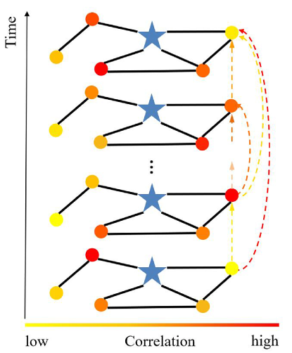
Complex spatial dependencies. Fig.1 demonstrates that the influence of different positions on the predicted position is different, and the influence of the same position on the predicted position is also varying with time. The spatial correlation between different positions is highly dynamic.
-
•
Dynamic temporal dependencies. The observed values at different times of the same position show non-linear changes, and the traffic state of the far time step sometimes has greater influence on the predicted time step than that of the recent time step, as shown in Fig.1. Meanwhile, [1] pointed out that traffic data usually presents periodicity, such as closeness, period and trend. Therefore, how to select the most relevant historical observations for prediction remains a challenging problem.
(2) External factors. Traffic spatio-temporal sequence data is also influenced by some external factors, such as weather conditions, events or road attributes.
Since traffic data shows strong dynamic correlation in both spatial and temporal dimensions, it is an important research topic to mine the non-linear and complicated spatial-temporal patterns, making accurate traffic predictions. Traffic prediction involves various application tasks. Here, we list the main application tasks of the existing traffic prediction work, which are as follows:
-
•
Flow
Traffic flow refers to the number of vehicles passing through a given point on the roadway in a certain period of time.
-
•
Speed
The actual speed of vehicles is defined as the distance it travels per unit of time. Most of the time, due to factors such as geographical location, traffic conditions, driving time, environment and personal circumstances of the driver, each vehicle on the roadway will have a speed that is somewhat different from those around it.
-
•
Demand
The problem is how to use historical requesting data to predict the number of requests for a region in a future time step, where the number of start/pick-up or end/drop-off is used as a representation of the demand in a region at a given time.
-
•
Travel time
In the case of obtaining the route of any two points in the road network, estimating the travel time is required. In general, the travel time should include the waiting time at the intersection.
-
•
Occupancy
The occupancy rate explains the extent to which vehicles occupy road space, and is an important indicator to measure whether roads are fully utilized.
Related surveys on traffic prediction There are a few recent surveys that have reviewed the literatures on traffic prediction in certain contexts from different perspectives. [2] reviewed the methods and applications from 2004 to 2013, and discussed ten challenges that were significant at the time. It is more focused on considering short-term traffic prediction and the literatures involved are mainly based on the traditional methods. Another work [3] also paid attention to short-term traffic prediction, which briefly introduced the techniques used in traffic prediction and gave some research suggestions. [4] provided sources of traffic data acquisition, and mainly focused on traditional machine learning methods. [5] outlined the significance and research directions of traffic prediction. [6] and [7] summarized relevant models based on classical methods and some early deep learning methods. Alexander et al. [8] presented a survey of deep neural network for traffic prediction. It discussed three common deep neural architectures, including convolutional neural network, recurrent neural network, and feedforward neural network. However, some recent advancements, e.g., graph-based deep learning, were not covered in [8]. [9] is an overview of graph-based deep learning architecture, with applications in the general traffic domain. [10] provided a survey focusing specifically on the use of deep learning models for analyzing traffic data. However, it only investigates the traffic flow prediction. In general, different traffic prediction tasks have common characteristics, and it is beneficial to consider them jointly. Therefore, there is still a lack of broad and systematic survey on exploring traffic prediction in general.
Our contributions To our knowledge, this is the first comprehensive survey on deep learning-based works in traffic prediction from multiple perspectives, including approaches, applications, datasets, experiments, analysis and future directions. Specifically, the contributions of this survey can be summarized as follows:
-
•
We first do a taxonomy for existing approaches, describing their key design choices.
-
•
We collect and summarize available traffic prediction datasets, which provide a useful pointer for other researches.
-
•
We perform a comparative experimental study to evaluate different models, identifying the most effective component.
-
•
We further discuss possible limitations of current solutions, and list promising future research directions.
A Taxonomy of Existing Approaches After years of efforts, the research on traffic prediction has achieved great progresses. In light of the development process, these methods can be broadly divided into two categories: classical methods and deep learning-based methods. Classical methods include statistical methods and traditional machine learning methods. The statistical method is to build a data-driven statistical model for prediction. The most representative algorithms are Historical Average (HA), Auto-Regressive Integrated Moving Average (ARIMA)[11], and Vector Auto-Regressive (VAR)[12]. Nevertheless, these methods require data to satisfy certain assumptions, and time-varying traffic data is too complex to satisfy these assumptions. Moreover, these methods are only applicable to relatively small datasets. Later, a number of traditional machine learning methods, such as Support Vector Regression (SVR)[13] and Random Forest Regression (RFR)[14], were proposed for traffic prediction problem. Such methods have the ability to process high-dimensional data and capture complex non-linear relationships.
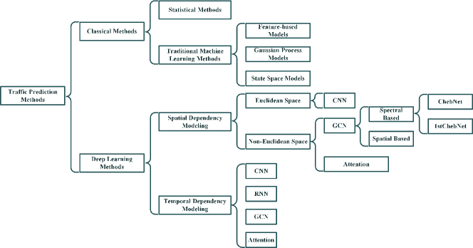
It was not until the advent of deep learning-based methods that the full potential of artificial intelligence in traffic prediction was developed [15]. This technology studies how to learn a hierarchical model to map the original input directly to the expected output [16]. In general, deep learning models stack up basic learnable blocks or layers to form a deep architecture, and the entire network is trained end-to-end. Several architectures have been developed to handle large-scale and complex spatio-temporal data. Generally, Convolutional Neural Network (CNN) [17] is employed to extract spatial correlation of the grid-structured data described by images or videos, and Graph Convolutional Network (GCN) [18] extends convolution operation to more general graph-structured data, which is more suitable to represent the traffic network structure. Furthermore, Recurrent Neural Network (RNN) [19, 20] and its variants LSTM [21] or GRU [22] are commonly utilized to model temporal dependency. Here, we summarize the key techniques commonly used in existing traffic prediction methods, as shown in Fig. 2.
Organization of this survey The rest of this paper is organized as follows. Section II covers the classical methods for traffic prediction. Section III reviews the work based on deep learning methods for traffic prediction, including the commonly used methods of modeling spatial correlation and temporal correlation, as well as some other new variants. Section IV lists some representative results in each task. Section V collects and organizes related datasets and commonly used external data types for traffic prediction. Section VI provides some comparisons and evaluates the performance of the relevant methods. Section VII discusses several significant and important directions of future traffic prediction. Finally, we conclude this paper in Section VIII.
II Classical Methods
Statistical and traditional machine learning models are two major representative data-driven methods for traffic prediction. In time-series analysis, autoregressive integrated moving average (ARIMA)[11] and its variants are one of the most consolidated approaches based on classical statistics and have been widely applied for traffic prediction problems ([11, 23, 24, 25, 26, 27] ). However, these methods are generally designed for small datasets, and are not suitable to deal with complex and dynamic time series data. In addition, since usually only temporal information is considered, the spatial dependency of traffic data is ignored or barely considered.
Traditional machine learning methods, which can model more complex data, are broadly divided into three categories: feature-based models, Gaussian process models and state space models. Feature-based methods solve traffic prediction problem ([28, 29, 30] ) by training a regression model based on human-engineered traffic features. These methods are simple to implement and can provide predictions in some practical situations. Gaussian process models the inner characteristics of traffic data through different kernel functions, which need to contain spatial and temporal correlations simultaneously. Although this kind of methods is proved to be effective and feasible in traffic prediction ([31, 32, 33] ), compared to feature-based models, they generally have higher computational load and storage pressure, which is not appropriate when a mass of training samples are available. State space models assume that the observations are generated by Markovian hidden states. The advantage of this model is that it can naturally model the uncertainty of the system and better capture the latent structure of the spatio-temporal data. However, the overall non-linearity of these models ([34, 35, 36, 37, 38, 39, 40, 41, 42, 43, 44, 45, 46, 47, 48] ) is limited, and most of the time they are not optimal for modeling complex and dynamic traffic data. Table I summarizes some recent representative classical approaches.
| Category | Application task | Approach | |
| Statistical methods | Flow | [11, 23, 26, 27] | |
| Demand | [24, 25] | ||
| Traditional machine learning methods | Feature-based models | Flow | [30] |
| Demand | [28, 29] | ||
| Gaussian process models | Flow | [31] | |
| Speed | [33] | ||
| Demand | [32] | ||
| Occupancy | [32] | ||
| State space models | Flow | [35, 39, 38, 34, 47, 48, 40, 45, 46] | |
| Speed | [42, 43, 36] | ||
| Demand | [37] | ||
| Travel time | [44] | ||
| Occupancy | [44, 41] | ||
III Deep Learning Methods
Deep learning models exploit much more features and complex architectures than the classical methods, and can achieve better performance. In Table II, we summarize the deep learning architectures in the existing traffic prediction literature, and we will review these commonly components in this section.
III-A Modeling Spatial Dependency
CNN. A series of studies have applied CNN to capture spatial correlations in traffic networks from two-dimensional spatio-temporal traffic data[3]. Since the traffic network is difficult to be described by 2D matrices, several researches try to convert the traffic network structure at different times into images and divide these images into standard grids, with each grid representing a region. In this way, CNNs can be used to learn spatial features among different regions.
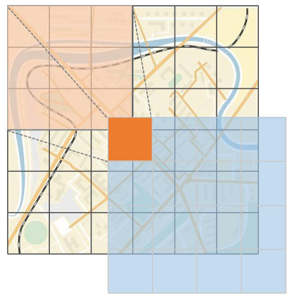
As shown in Fig. 3, each region is directly connected to its nearby regions. With a window, the neighborhood of each region is its surrounding eight regions. The positions of these eight regions indicate an ordering of a region’s neighbors. A filter is then applied to this patch by taking the weighted average of the central region and its neighbors across each channel. Due to the specific ordering of neighboring regions, the trainable weights are able to be shared across different locations.
In the division of traffic road network structure, there are many different definitions of positions according to different granularity and semantic meanings. [1] divided a city into I J grid maps based on the longitude and latitude where a grid represented a region. Then, a CNN was applied to extract the spatial correlation between different regions for traffic flow prediction.
GCN. Traditional CNN is limited to modeling Euclidean data, and GCN is therefore used to model non-Euclidean spatial structure data, which is more in line with the structure of traffic road network. GCN generally consists of two type of methods, spectral-based and spatial-based methods. Spectral-based approaches define graph convolutions by introducing filters from the perspective of graph signal processing where the graph convolution operation is interpreted as removing noise from graph signals. Spatial-based approaches formulate graph convolutions as aggregating feature information from neighbors. In the following, we will introduce spectral-based GCNs and spatial-based GCNs respectively.
(1) Spectral Methods. Bruna et al. [18] first developed spectral network, which performed convolution operation for graph data from spectral domain by computing the eigen-decomposition of the graph Laplacian matrix . Specifically, the graph convolution operation of a signal with a filter can be defined as:
| (1) |
where is the matrix of eigenvectors of normalized graph Laplacian , which is defined as , is the diagonal matrix, , is the adjacency matrix of the graph, is the diagonal matrix of eigenvalues, . If we denote a filter as parameterized by , the graph convolution can be simplified as:
| (2) |
where a graph signal is filtered by with multiplication between and graph transform . Though the computation of filter in graph convolution can be expensive due to multiplications with matrix , two approximation strategies have been successively proposed to solve this issue.
ChebNet. Defferrard et al. [49] introduced a filter as Chebyshev polynomials of the diagonal matrix of eigenvalues, i.e, , where is now a vector of Chebyshev coefficients, , and denotes the largest eigenvalue. The Chebyshev polynomials are defined as with and . Then, the convolution operation of a graph signal with the defined filter is:
| (3) | ||||
where .
First order of ChebNet (1stChebNet). An first-order approximation of ChebNet introduced by Kipf and Welling [50] further simplified the filtering by assuming and , we can obtain the following simplified expression:
| (4) |
where and are learnable parameters. After further assuming these two free parameters with . This can be obtained equivalently in the following matrix form:
| (5) |
To avoid numerical instabilities and exploding/vanishing gradients due to stack operations, another normalization technique is introduced: , with and . Finally, a graph convolution operation can be changed to:
| (6) |
where is a signal, is a matrix of filter parameters, is the input channels, is the number of filters, and is the transformed signal matrix.
To fully utilize spatial information, [51] modeled the traffic network as a general graph rather than treating it as grids, where the monitoring stations in a traffic network represent the nodes in the graph, the connections between stations represent the edges, and the adjacency matrix is computed based on the distances among stations, which is a natural and reasonable way to formulate the road network. Afterwards, two graph convolution approximation strategies based on spectral methods were used to extract patterns and features in the spatial domain, and the computational complexity was also reduced. [52] first used graphs to encode different kinds of correlations among regions, including neighborhood, functional similarity, and transportation connectivity. Then, three groups of GCN based on ChebNet were used to model spatial correlations respectively, and traffic demand prediction was made after further integrating temporal information.
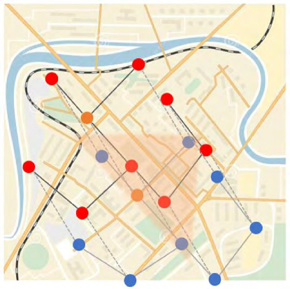
(2) Spatial Methods. Spatial methods define convolutions directly on the graph through the aggregation process that operates on the central node and its neighbors to obtain a new representation of the central node, as depicted by Fig.4. In [53], traffic network was firstly modeled as a directed graph, the dynamics of the traffic flow was captured based on the diffusion process. Then a diffusion convolution operation is applied to model the spatial correlation, which is a more intuitive interpretation and proves to be effective in spatial-temporal modeling. Specifically, diffusion convolution models the bidirectional diffusion process, enabling the model to capture the influence of upstream and downstream traffic. This process can be defined as:
| (7) |
where is the input, represents the number of input features of each node. denotes the diffusion convolution, is the diffusion step, is a filter and are learnable parameters. and are out-degree and in-degree matrices respectively. To allow multiple input and output channels, DCRNN [53] proposes a diffusion convolution layer, defined as:
| (8) |
where is the output, parameterizes the convolutional filter , is the number of output features, is the activation function. Based on the diffusion convolution process, [54] designed a new neural network layer that can map the transformation of different dimensional features and extract patterns and features in spatial domain. [55] modified the diffusion process in [53] by utilizing a self-adaptive adjacency matrix, which allowed the model to mine hidden spatial dependency by itself. [56] introduced the notion of aggregation to define graph convolution. This operation can assemble the features of each node with its neighbors. The aggregate function is a linear combination whose weights are equal to the weights of the edges between the node and its neighbors. This graph convolutional operation can be expressed as follow:
| (9) |
where is the input of the -th graph convolutional layer, and are parameters, and is the activation function.
Attention. Attention mechanism is first proposed for natural language processing[57], and has been widely used in various fields. The traffic condition of a road is affected by other roads with different impacts. Such impact is highly dynamic, changing over time. To model these properties, the spatial attention mechanism is often used to adaptively capture the correlations between regions in the road network ([58, 59, 60, 61, 62, 63, 64, 65, 66] ). The key idea is to dynamically assign different weights to different regions at different time steps. For the sake of simplicity, we ignore time coordinates for the moment. Attention mechanism operates on a set of input sequence with elements where , and computes a new sequence with the same length where . Each output element is computed as a weighted sum of a linear transformed input elements:
| (10) |
The weight coefficient indicates the importance of to , and it is computed by a softmax function:
| (11) |
where is computed using a compatibility function that compares two input elements:
| (12) |
and generally Perceptron is chosen for the compatibility function. Here, the learnable parameters are , , and . This mechanism has proven effective, but when the number of elements in a sequence is large, we need to calculate weight coefficients, and therefore the time and memory consumption are heavy.
In traffic speed prediction, [60] used attention mechanism to dynamically capture the spatial correlation between the target region and the first-order neighboring regions of the road network. [67] combined the GCN based on ChebNet with attention mechanism to make full use of the topological properties of the traffic network and dynamically adjust the correlations between different regions.
III-B Modeling Temporal Dependency
CNN. [68] first introduced the fully convolutional model for sequence to sequence learning. A representative work in traffic research, [51] applied purely convolutional structures to simultaneously extract spatio-temporal features from graph-structured time series data. In addition, dilated causal convolution is a special kind of standard one-dimensional convolution. It adjusts the size of the receptive field by changing the value of the dilation rate, which is conducive to capture the long-term periodic dependence. [69] and [70] therefore adopted the dilated causal convolution as the temporal convolution layer of their models to capture a node’s temporal trends. Compared to recurrent models, convolutions create representations for fixed size contexts, however, the effective context size of the network can easily be made larger by stacking several layers on top of each other. This allows to precisely control the maximum length of dependencies to be modeled. The convolutional network does not rely on the calculation of the previous time step, so it allows parallelization of every element in the sequence, which can make better use of GPU hardware, and easier to optimize. This is superior to RNNs, which maintain the entire hidden state of the past, preventing parallel calculations in a sequence.
RNN. RNN and its variant LSTM or GRU, are neural networks for processing sequential data. To model the non-linear temporal dependency of traffic data, RNN-based approaches have been applied to traffic prediction[3]. These models rely on the order of data to process data in turn, and therefore one disadvantage of these models is that when modeling long sequences, their ability to remember what they learned before many time steps may decline.
In RNN-based sequence learning, a special network structure known as encoder-decoder has been applied for traffic prediction ( [71, 61, 72, 53, 73, 74, 62, 75, 76, 77, 63, 78, 58, 79, 64, 65, 66] ). The key idea is to encode the source sequence as a fixed-length vector and use the decoder to generate the prediction.
| (13) |
| (14) |
where is the encoder and is the decoder. denotes the input information available at timestamp , is a transformed semantic vector representation, is the value of -step-ahead prediction, and are learning parameters.
One potential problem with encoder-decoder structure is that regardless of the length of the input and output sequences, the length of semantic vector between encoding and decoding is always fixed, and therefore when the input information is too long, some information will be lost.
Attention. To resolve the above issue, an important extension is to use an attention mechanism on time axis, which can adaptively select the relevant hidden states of the encoder to produce output sequence. This is similar to attention in the spatial methods. Such a temporal attention mechanism can not only model the non-linear correlation between the current traffic condition and the previous observations at a certain position in the road network, but also model the long-term sequence data to solve the deficiencies of RNN.
[62] designed a temporal attention mechanism to adaptively model the non-linear correlations between different time steps. [67] incorporated a standard convolution and attention mechanism to update the information of a node by fusing the information at the neighboring time steps, and semantically express the dependency intensity between different time steps. Considering that traffic data is highly periodic, but not strictly periodic, [80] designed a periodically shifted attention mechanism to deal with long-term periodic dependency and periodic temporal shifting.
GCN. Song et al. first constructed a localized spatio-temporal graph that includes both temporal and spatial attributes, and then used the proposed spatial-based GCN method to model the spatio-temporal correlations simultaneously [56].
III-C Joint Spatio-Temporal Relationships Modeling
As shown in Table II, most methods use a hybrid deep learning framework, which combines different types of techniques to capture the spatial dependencies and temporal correlations of traffic data separately. They assume that the relations of geographic information and temporal information are independent and do not consider their joint relations. Therefore, the spatial and temporal correlations are not fully exploited to obtain better accuracy. To solve this limitation, researchers have attempted to integrate spatial and temporal information into an adjacency graph matrix or tensor. For example, [56] got a localized spatio-temporal graph by connecting all nodes with themselves at the previous moment and the next moment. According to the topological structure of the localized spatial-temporal graph, the correlations between each node and its spatio-temporal neighbors can be captured directly. In [81], Fang et al. constructed three matrices for the historical traffic conditions of different links, the features of the neighbor links, and the features of the historical time slots, in which each row of the matrix corresponds to the information of a link. Finally, these three matrices were concatenated into a matrix and reshaped into a 3D spatio-temporal tensor. Attention mechanism was then used to obtain the relations between the traffic conditions.
III-D Deep Learning plus Classical Models
Recently, more and more researches are combining deep learning with classical methods, and some advanced methods have been used in traffic prediction ([82, 83, 84, 85] ). This kind of method not only makes up for the weak ability of non-linear representation of classical models but also makes up for the poor interpretability of deep learning methods. [82] proposed a method based on the generation model of state space and the inference model based on filtering, using deep neural networks to realize the non-linearity of the emission and the transition models, and using the recurrent neural network to realize the dependence over time. Such a non-linear network based parameterization provides the flexibility to deal with arbitrary data distribution. [83] proposed a deep learning framework that introduced matrix factorization method into deep learning model, which can model the latent region functions along with the correlations among regions, and further improve the model capability of the citywide flow prediction. [84] developed a hybrid model that associated a global matrix decomposition model regularized by a temporal deep network with a local deep temporal model that captured patterns specific to each dimension. Global and local models are combined through a data-driven attention mechanism for each dimension. Therefore, global patterns of the data can be utilized and combined with local calibration for better prediction. [85] combined a latent model and multi-layer perceptrons (MLP) to design a network for addressing multivariate spatio-temporal time series prediction problems. The model captures the dynamics and correlations of multiple series at the spatial and temporal levels. Table III summarizes relevant literatures in terms of deep learning plus classical methods.
III-E Limitations of the Deep Learning-based Method
The strengths of the deep neural network model make it very attractive and indeed greatly promote the progress in the field of traffic prediction. However, it also possess several disadvantages compared with classical methods.
-
•
High data demand. Deep learning is highly data-dependent, and typically the larger the amount of data, the better it performs. In many cases, such data is not readily available, for example, some cities may release taxi data for multiple years, while others release data for just a few days.
-
•
High computational complexity. Deep learning requires high computing power, and ordinary CPUs can no longer meet the requirements of deep learning. The mainstream computing uses GPU and TPU. At the same time, with the increase of model complexity and the number of parameters, the demand for memory is also gradually increasing. In general, deep neural networks are more computationally expensive than classical algorithms.
-
•
Lack of interpretability. Deep learning models are mostly considered as “black-boxs” that lack interpretability. In general, the prediction accuracy of deep learning models is higher than that of classical methods. However, there is no explanation as to why these results are obtained or how parameters can be determined to make the results better.
IV Representative Results
| Application task | Spatial modeling type | Temporal modeling type | Approach | |
| Flow | CNN | – | [86, 1, 87, 88, 89, 90] | |
| RNN | [70, 91, 92, 93, 74, 94] | |||
| 1stChebNet | RNN | [79, 95] | ||
| ChebNet | CNN (Causal CNN) | [69] | ||
| RNN | [96] | |||
| GCN+Attention | CNN (1-D Conv) +Attention | [67] | ||
| Attention only | – | [97] | ||
| RNN | [58] | |||
| RNN+Attention | [65, 66] | |||
| Attention only | [62] | |||
| Speed | – | RNN | [98, 99] | |
| CNN | RNN | [100, 101] | ||
| 1stChebNet | CNN (1-D Conv) | [51] | ||
| RNN | [102] | |||
| ChebNet | CNN | (1-D Conv) | [51] | |
| (2-D Conv) | [103] | |||
| RNN | [73, 104, 96, 105] | |||
| RNN+Attention | [75] | |||
| GCN(spatial-based) | CNN (Causal CNN) | [55] | ||
| RNN | [53, 54] | |||
| GCN+Attention | CNN (1-D Conv) | [106] | ||
| RNN | [107] | |||
| Attention only | RNN | [60, 58] | ||
| Attention only | [62, 63] | |||
| Demand | – | RNN | [108] | |
| CNN | – | [109] | ||
| RNN | [110, 72, 111, 112] | |||
| RNN+Attention | [80] | |||
| 1stChebNet | Attention only | [77] | ||
| RNN | [76, 113] | |||
| ChebNet | RNN | [52] | ||
| Attention only | RNN | [59] | ||
| Attention only | [64, 61] | |||
| Travel time | – | RNN | [114, 115] | |
| CNN | RNN | [116] | ||
| ChebNet | CNN (1-D Conv) | [117] | ||
| Occupancy | – | RNN | [78] | |
| CNN | RNN | [118] | ||
| Application task | Approach | Spatio-temporal modeling |
| Flow | [85] | State space model+MLP |
| [83] | State space model+CNN+RNN | |
| Demand | [83] | State space model+CNN+RNN |
| Occupancy | [82] | State space model+RNN |
| [84] | State space model+CNN |
In this section, we summarize some representative results of different application tasks. Based on the literature studied on different tasks, we list the current best performance methods under commonly used public datasets, as shown in Table IV. We can have the following observations: First, the results on different datasets vary greatly under the same prediction task. For example, in the demand prediction task, the NYC Taxi and TaxiBJ datasets obtained the accuracy of 8.385 and 17.24, respectively, under the same time interval and prediction time. Under the same condition of the prediction task and the dataset, the performance decreases with the increase of prediction time, as shown in the speed prediction results on Q-Traffic. For the dataset of the same data source, due to the different time and region selected, it also has a greater impact on the accuracy, e.g., related datasets based on PeMS under the speed prediction task. Second, in different prediction tasks, the accuracy of speed prediction task can reach above 90% in general, which is significantly higher than other tasks whose accuracy rate is close to or more than 80%. Therefore, there is still much room for improvement in these tasks.
| Application task | Dataset | Time interval | Prediction window | MAPE | RMSE |
| Flow | TaxiBJ | 30min | 30min | 25.97%[90] | 15.88[90] |
| PeMSD3 | 5min | 60min | 16.78%[56] | 29.21[56] | |
| PeMSD4 | 5min | 60min | 11.09%[65] | 31.00[65] | |
| PEMS07 | 5min | 60min | 10.21%[56] | 38.58[53] | |
| PeMSD8 | 5min | 60min | 8.31%[65] | 24.74[65] | |
| NYC Bike | 60min | 60min | – | 6.33[87] | |
| T-Drive | 60min | 60/120/180min | – | 29.9/34.7/37.1[58] | |
| Speed | METR-LA | 5min | 5/15/30/60min | 4.90%[54]/6.80%/8.30%/10.00%[107] | 3.57[54]/5.12/6.17/7.30[107] |
| PeMS-BAY | 5min | 15/30/60min | 2.73%[55]/3.63%[62]/4.31%[62] | 2.74[55]/3.70[55]/4.32[62] | |
| PeMSD4 | 5min | 15/30/45/60min | 2.68%[53]/3.71%[53]/4.42%/4.85%[106] | 2.93/3.92/4.47/4.83[106] | |
| PeMSD7 | 5min | 15/30/45/60min | 5.14%/7.18%/8.51%/9.60%[106] | 3.98/5.47/6.39/7.09[106] | |
| PeMSD7(M) | 5min | 15/30/45min | 5.24%/7.33%/8.69%[51] | 4.04/5.70/6.77[51] | |
| PeMSD8 | 5min | 15/30/45/60min | 2.24%/3.02%/3.51%/3.89%[106] | 2.45/3.28/3.75/4.11[106] | |
| SZ-taxi | 15min | 15/30/45/60min | – | 3.92/3.96/3.98/4.00[102] | |
| Los-loop | 5min | 15/30/45/60min | – | 5.12/6.05/6.70/7.26[102] | |
| LOOP | 5min | 5min | 6.01%[105] | 4.63[105] | |
| Q-Traffic | 15min | 15/30/45/60/ 75/90/105/120min | 4.52%/7.93%/8.89%/9.24%/ 9.43%/9.56%/9.69%/9.78% [73] | – | |
| Demand | NYC Taxi | 30min | 30min | – | 8.38[72] |
| NYC Bike | 60min | 60min | 21.00%[77] | 4.51[77] | |
| TaxiBJ | 30min | 30min | 13.80%[77] | 17.24[77] | |
| Travel time | Chengdu | – | – | 11.89%[116] | – |
| Occupancy | PeMSD-SF | 60min | 7 rolling time windows (24 time-points at a time) | 16.80%[84] | – |
Some companies are currently conducting intelligent transportation research, such as amap, DiDi, and Baidu maps. According to amap technology annual in 2019[119], amap has carried out the exploration and practice of deep learning in the prediction of the historical speed of amap driving navigation, which is different from the common historical average method and takes into account the timeliness and annual periodicity characteristics presented in the historical data. By introducing the Temporal Convolutional Network (TCN) [120] model for industrial practice, and combining feature engineering (extracting dynamic and static features, introducing annual periodicity, etc.), the shortcomings of existing models are successfully solved. The arrival time of a given week is measured based on the order data, and it has a badcase rate of 10.1%, which is 0.9% lower than the baseline. For the travel time prediction in the next hour, [117] designed a multi-model architecture to infer the future travel time by adding contextual information using the upcoming traffic flow data. Using anonymous user data from amap, MAPE can be reduced to around 16% in Beijing.
The Estimated Time of Arrival (ETA), supply and demand and speed prediction are the key technologies in DiDi’s platform. DiDi has applied artificial intelligence technology in ETA, reduced MAPE index to 11% by utilizing neural network and DiDi’s massive order data, and realized the ability to provide users with accurate expectation of arrival time and multi-strategy path planning under real-time large-scale requests. In the prediction and scheduling, DiDi has used deep learning model to predict the difference between supply and demand after some time in the future, and provided driver scheduling service. The prediction accuracy of the gap between supply and demand in the next 30 minutes has reached 85%. In the urban road speed prediction task, DiDi proposed a prediction model based on driving trajectory calibration[121]. Through comparison experiments based on Chengdu and Xi’an data in the DiDi gaia dataset, it was concluded that the overall MSE indicator for speed prediction was reduced to 3.8 and 3.4.
Baidu has solved the traffic prediction task of online route queries by integrating auxiliary information into deep learning technology, and released a large-scale traffic prediction dataset from Baidu Map with offline and online auxiliary information[73]. The overall MAPE and 2-hour MAPE of speed prediction on this dataset decreased to 8.63% and 9.78%, respectively. In [81], the researchers proposed an end-to-end neural framework as an industrial solution for the travel time prediction function in mobile map applications, aiming at exploration of spatio-temporal relation and contextual information in traffic prediction. The MAPE in Taiyuan, Hefei and Huizhou, sampled on the Baidu maps, can be reduced to 21.79%, 25.99% and 27.10% respectively, which proves the superiority of the model. The model is already in production on Baidu maps and successfully handles tens of billions of requests a day.
V Public datasets
High-quality datasets are essential for accurate traffic forecasting. In this section, we comprehensively summarize the public data information used for the prediction task, which mainly consists of two parts: one is the public spatio-temporal sequence data commonly used in the prediction, and the other is the external data to improve the prediction accuracy. However, the latter data is not used by all models due to the design of different model frameworks or the availability of the data.
Public datasets Here, we list public, commonly used and large-scale real-world datasets in traffic prediction.
-
•
PeMS: It is an abbreviation from the California Transportation Agency Performance Measurement System (PeMS), which is displayed on the map and collected in real-time by more than 39000 independent detectors. These sensors span the freeway system across all major metropolitan areas of the State of California. The source is available at: http://pems.dot.ca.gov/. Based on this system, several sub-dataset versions (PeMSD3/4/7(M)/7/8/-SF/-BAY) have appeared and are widely used. The main difference is the range of time and space, as well as the number of sensors included in the data collection.
PeMSD3: This dataset is a piece of data processed by Song et al. It includes 358 sensors and flow information from 9/1/2018 to 11/30/2018. A processed version is available at: https://github.com/Davidham3/STSGCN.
PeMSD4: It describes the San Francisco Bay Area, and contains 3848 sensors on 29 roads dated from 1/1/2018 until 2/28/2018, 59 days in total. A processed version is available at: https://github.com/Davidham3/ASTGCN/tree/master/data/ PEMS04.
PeMSD7(M): It describes the District 7 of California containing 228 stations, and The time range of it is in the weekdays of May and June of 2012. A processed version is available at: https://github.com/Davidham3/STGCN/tree/master/ datasets.
PeMSD7: This version was publicly released by Song et al. It contains traffic flow information from 883 sensor stations, covering the period from 7/1/2016 to 8/31/2016. A processed version is available at: https://github.com/Davidham3/STSGCN.
PeMSD8: It depicts the San Bernardino Area, and contains 1979 sensors on 8 roads dated from 7/1/2016 until 8/31/2016, 62 days in total. A processed version is available at: https://github.com/Davidham3/ASTGCN/tree/master/ data/PEMS08.
PeMSD-SF: This dataset describes the occupancy rate, between 0 and 1, of different car lanes of San Francisco bay area freeways. The time span of these measurements is from 1/1/2008 to 3/30/2009 and the data is sampled every 10 minutes. The source is available at: http://archive.ics.uci.edu/ml/datasets/PEMS-SF.
PeMSD-BAY: It contains 6 months of statistics on traffic speed, ranging from 1/1/2017 to 6/30/2017, including 325 sensors in the Bay area. The source is available at: https://github.com/liyaguang/DCRNN.
-
•
METR-LA: It records four months of statistics on traffic speed, ranging from 3/1/2012 to 6/30/2012, including 207 sensors on the highways of Los Angeles County. The source is available at: https://github.com/liyaguang/DCRNN.
-
•
LOOP: It is collected from loop detectors deployed on four connected freeways (I-5, I-405, I-90 and SR-520) in the Greater Seattle Area. It contains traffic state data from 323 sensor stations over the entirely of 2015 at 5-minute intervals. The source is available at: https://github.com/zhiyongc/Seattle-Loop-Data.
-
•
Los-loop: This dataset is collected in the highway of Los Angeles County in real time by loop detectors. It includes 207 sensors and its traffic speed is collected from 3/1/2012 to 3/7/2012. These traffic speed data is aggregated every 5 minutes. The source is available at: https://github.com/lehaifeng/T-GCN/tree/master/data.
-
•
TaxiBJ: Trajectory data is the taxicab GPS data and meteorology data in Beijing from four time intervals: 1st Jul. 2013 - 30th Otc. 2013, 1st Mar. 2014 - 30th Jun. 2014, 1st Mar. 2015 - 30th Jun. 2015, 1st Nov. 2015 - 10th Apr. 2016. The source is available at: https://github.com/lucktroy/DeepST/tree/master/ data/TaxiBJ.
-
•
SZ-taxi: This is the taxi trajectory of Shenzhen from Jan.1 to Jan.31, 2015. It contains 156 major roads of Luohu District as the study area. The speed of traffic on each road is calculated every 15 minutes. The source is available at: https://github.com/lehaifeng/T-GCN/tree/master/data.
-
•
NYC Bike: The bike trajectories are collected from NYC CitiBike system. There are about 13000 bikes and 800 stations in total. The source is available at: https://www.citibikenyc.com/system-data. A processed version is available at: https://github.com/lucktroy/DeepST/tree/master/data/ BikeNYC.
-
•
NYC Taxi: The trajectory data is taxi GPS data for New York City from 2009 to 2018. The source is available at: https://www1.nyc.gov/site/tlc/about/tlc-trip-record-data.page.
-
•
Q-Traffic dataset: It consists of three sub-datasets: query sub-dataset, traffic speed sub-dataset and road network sub-dataset. These data are collected in Beijing, China between April 1, 2017 and May 31, 2017, from the Baidu Map. The source is available at: https://github.com/JingqingZ/BaiduTraffic#Dataset.
-
•
Chicago: This is the trajectory of shared bikes in Chicago from 2013 to 2018. The source is available at: https://www.divvybikes.com/system-data.
-
•
BikeDC: It is taken from the Washington D.C.Bike System. The dataset includes data from 472 stations and four time intervals of 2011, 2012, 2014 and 2016. The source is available at: https://www.capitalbikeshare.com/system-data.
-
•
ENG-HW: It contains traffic flow information from inter-city highways between three cities, recorded by British Government, with a time range of 2006 to 2014. The source is available at: http://tris.highwaysengland.co.uk/detail/trafficflowdata.
-
•
T-Drive: It consists of tremendous amounts of trajectories of Beijing taxicabs from Feb.1st, 2015 to Jun. 2nd 2015. These trajectories can be used to calculate the traffic flow in each region. The source is available at: https://www.microsoft.com/en-us/research/publication/t-drive-driving-directions-based-on-taxi-trajectories/.
-
•
I-80: It is collected detailed vehicle trajectory data on eastbound I-80 in the San Francisco Bay area in Emeryville, CA, on April 13, 2005. The dataset is 45 minutes long, and the vehicle trajectory data provides the precise location of each vehicle in the study area every tenth of a second. The source is available at: http://ops.fhwa.dot.gov/trafficanalysistools/ngsim.htm.
-
•
DiDi chuxing: DiDi gaia data open program provides real and free desensitization data resources to the academic community. It mainly includes travel time index, travel and trajectory datasets of multiple cities. The source is available at: https://gaia.didichuxing.com.
-
•
Travel Time Index data:
The dataset includes the travel time index of Shenzhen, Suzhou, Jinan, and Haikou, including travel time index and average driving speed of city-level, district-level, and road-level, and time range is from 1/1/2018 to 12/31/2018. It also includes the trajectory data of the Didi taxi platform from 10/1/2018 to 12/1/2018 in the second ring road area of Chengdu and Xi’an, as well as travel time index and average driving speed of road-level in the region, and Chengdu and Xi’an city-level. Moreover, the city-level, district-level, road-level travel time index and average driving speed of Chengdu and Xi’an from 1/1/2018 to 12/31/2018 is contained.
Travel data:
This dataset contains daily order data from 5/1/2017 to 10/31/2017 in Haikou City, including the latitude and longitude of the start and end of the order, as well as the order attribute of the order type, travel category, and number of passengers.
Trajectory data:
This dataset comes from the order driver trajectory data of the Didi taxi platform in October and November 2016 in the Second Ring Area of Xi’an and Chengdu. The trajectory point collection interval is 2-4s. The trajectory points have been processed for road binding, ensuring that the data corresponds to the actual road information. The driver and order information were encrypted, desensitized and anonymized.
Common external data Traffic prediction is often influenced by a number of complex factors, which are usually called external data. Here, we list common external data items.
-
•
Weather condition: temperature, humidity, wind speed, visibility and weather state (sunny/rainy/windy/cloudy etc.)
-
•
Driver ID:
Due to the different personal conditions of drivers, the prediction will have a certain impact, therefore, it is necessary to label the driver, and this information is mainly used for personal prediction.
-
•
Event: It includes various holidays, traffic control, traffic accidents, sports events, concerts and other activities.
-
•
Time information: day-of-week, time-of-day.
(1) day-of-week usually includes weekdays and weekends due to the distinguished properties.
(2) time-of-day generally has two division methods, one is to empirically examine the distribution with respect to time in the training dataset, 24 hours in each day can be intuitively divided into 3 periods: peak hours, off-peak hours, and sleep hours. The other is to manually divide one day into several timeslots, each timeslot corresponds to an interval.
VI Experimental analysis and discussions
In this section, we conduct experimental studies for several deep learning based traffic prediction methods, to identify the key components in each model. To this end, we utilize METR-LA dataset for speed prediction, evaluate the state-of-the-art approaches with public codes on this dataset, and investigate the performance limits.
VI-A Experimental Setup
In the experiment, we compare the performance of six typical speed prediction methods with public codes on a public dataset. Table V summarizes the links of public source codes for related comparison methods.
| Approach | Link |
| STGCN[51] | https://github.com/VeritasYin/STGCN_IJCAI-18 |
| DCRNN[53] | https://github.com/liyaguang/DCRNN |
| ASTGCN[67] | https://github.com/guoshnBJTU/ASTGCN-r-pytorch |
| Graph WaveNet[55] | https://github.com/nnzhan/Graph-WaveNet |
| STSGCN[56] | https://github.com/Davidham3/STSGCN |
| GMAN[62] | https://github.com/zhengchuanpan/GMAN |
METR-LA dataset: This dataset contains 207 sensors and collects 4 months of data ranging from Mar 1st 2012 to Jun 30th 2012 for the experiment. 70% of data is used for training, 20% is used for testing while the remaining 10% for validation. Traffic speed readings are aggregated into 5 minutes windows, and Z-Score is applied for normalization. To construct the road network graph, each traffic sensor is considered as a node, and the adjacency matrix of the nodes is constructed by road network distance with a thresholded Gaussian kernel[122].
We use the following three metrics to evaluate different models: Mean Absolute Error (MAE), Rooted Mean Squared Error (RMSE), and Mean Absolute Percent Error (MAPE).
| (15) |
| (16) |
| (17) |
where and denote the predicted value and the ground truth of region for predicted time step, and is the total number of samples.
For hyperparameter settings in the comparison algorithms, we set their values according to the experiments in the corresponding literatures ( [51, 53, 67, 55, 62, 56] ).
| Metric | STGCN | DCRNN | ASTGCN | Graph WaveNet | STSGCN | GMAN | ||
| METR-LA | 15min | MAE | 2.88 | 2.77 | 4.86 | 2.69 | 3.01 | 2.77 |
| RMSE | 5.74 | 5.38 | 9.27 | 5.15 | 6.69 | 5.48 | ||
| MAPE | 7.62% | 7.30% | 9.21% | 6.90% | 7.27% | 7.25% | ||
| 30min | MAE | 3.47 | 3.15 | 5.43 | 3.07 | 3.42 | 3.07 | |
| RMSE | 7.24 | 6.45 | 10.61 | 6.22 | 7.93 | 6.34 | ||
| MAPE | 9.57% | 8.80% | 10.13% | 8.37% | 8.49% | 8.35% | ||
| 60min | MAE | 4.59 | 3.60 | 6.51 | 3.53 | 4.09 | 3.40 | |
| RMSE | 9.40 | 7.59 | 12.52 | 7.37 | 9.65 | 7.21 | ||
| MAPE | 12.70% | 10.50% | 11.64% | 10.01% | 10.44% | 9.72% |
VI-B Experimental Results and Analysis
In this section, we evaluate the performance of various advanced traffic speed prediction methods on the graph-structured data, and the prediction results in the next 15 minute, 30 minute, and 60 minute (=3, 6, 12) are shown in Table VI.
STGCN applied ChebNet graph convolution and 1D convolution to extract spatial dependencies and temporal correlations. ASTGCN leveraged two attention layers on the basis of STGCN to capture the dynamic correlations of traffic network in spatial dimension and temporal dimension, respectively. DCRNN was a cutting edge deep learning model for prediction, which used diffusion graph convolutional networks and RNN during training stage to learn the representations of spatial dependencies and temporal relations. Graph WaveNet combined graph convolution with dilated casual convolution to capture spatial-temporal dependencies. STSGCN simultaneously extracted localized spatio-temporal correlation information based on the adjacency matrix of localized spatio-temporal graph. GMAN used purely attention structures in spatial and temporal dimensions to model dynamic spatio-temporal correlations.
As can be seen from the experimental results in Table VI: First, the attention-based methods (GMAN) perform better than other GCN-based methods in extracting spatial correlations. When modeling spatial correlations, GCN uses sum, mean or max functions to aggregate the features of each node’s neighbors, ignoring the relative importance of different neighbors. On the contrary, the attention mechanism introduces the idea of weighting to realize adaptive updating of nodes at different times according to the importance of neighbor information, leading to better results. Second, the performance of the spectral models (STGCN and ASTGCN) is generally lower than that of the spatial models (DCRNN, Graph WaveNet and STSGCN). In addition, the results of most methods are not significantly different for 15min, but with the increase of the predicted time length, the performance of the attention-based method (GMAN) is significantly better than other GCN-based methods. Since most existing methods predict traffic conditions in an iterative manner, and their performance may not be greatly affected in short-term predictions because all historical observations used for prediction are error-free. However, as long-term prediction has to produce the results conditioned on previous predictions, resulting in error accumulations and reducing the accuracy of prediction greatly. Since the attention mechanism can directly perform multi-step predictions, ground-truth historical observations can be used regardless of short-term or long-term predictions, without the need to use error-prone values. Therefore, the above observations suggest possible ways to improve the prediction accuracy. First, the attention mechanism can extract the spatial information of road network more effectively. Second, the spatial-based approaches are generally more efficient than the spectral-based approaches when working with GCN. Third, the attention mechanism is more effective to improving the performance of long-term prediction when modeling temporal correlation. It is worth mentioning that adding an external data component is also beneficial for performance when external data is available.
VI-C Computational complexity
To evaluate the computation complexity, we compare the computation time and the number of parameters among these models on the METR-LA dataset. All the experiments are conducted on the Tesla K80 with 12GB memory, the batchsize of each method is uniformly set to 64, is set to 12, and we report the average training time of one epoch. For inference, we compute the time cost on the validation data. The results are shown in Table VII. STGCN adopts fully convolutional structures so that it is the fastest in training, and DRCNN uses the recurrent structures, which are very time consuming. Compared to methods (e.g., STGCN, DCRNN, ASTGCN, STSGCN) that require iterative calculations to generate 12 predicted results, Graph WaveNet can predict 12 steps ahead of time in one run, thus requiring less time for inference. STSGCN integrates three graphs at different moments into one graph as the adjacency matrix, which greatly increases the number of model parameters. Since GMAN is a pure attention mechanism model that consists of multiple attention mechanisms, it is necessary to calculate the relation between pairs of multiple variables, so the number of parameters is also high. Note that, when calculating the computation time of GMAN, it displays “out of memory” on our device, due to the relatively complex design of the model.
| Method | Computation time | Number of parameters | |
| Training(s/epoch) | Inference(s) | ||
| STGCN | 49.24 | 28.13 | 320143 |
| DCRNN | 775.31 | 56.09 | 372352 |
| ASTGCN | 570.34 | 25.51 | 262379 |
| Graph WaveNet | 234.82 | 11.89 | 309400 |
| STSGCN | 560.29 | 25.56 | 1921886 |
| GMAN | – | – | 900801 |
VII Future Directions
Although traffic prediction has made great progress in recent years, there are still many open challenges that have not been fully investigated. These issues need to be addressed in future work. In the following discussion, we will state some future directions for further researches.
-
•
Few shot problem: Most existing solutions are data intensive. However, abnormal conditions (extreme weather, temporary traffic control, etc) are usually non-recurrent, it is difficult to obtain data, which makes the training sample size smaller and learning more difficult than that under normal traffic conditions. In addition, due to the uneven development level of different cities, many cities have the problem of insufficient data. However, sufficient data is usually a prerequisite for deep learning methods. One possible solution to this problem is to use transfer learning techniques to perform deep spatio-temporal prediction tasks across cities. This technology aims to effectively transfer knowledge from a data-rich source city to a data-scarce target city. Although recent approaches have been proposed ([70, 123, 91, 124] ), these researches have not been thoroughly studied, such as how to design a high-quality mathematical model to match two regions, or how to integrate other available auxiliary data sources, etc., are still worth considering and investigating.
-
•
Knowledge graph fusion: Knowledge graph is an important tool for knowledge integration. It is a complex relational network composed of a large number of concepts, entities, entity relations and attributes. Transportation domain knowledge is hidden in multi-source and massive traffic big data. The construction, learning and deep knowledge search of large-scale transportation knowledge graph can help to dig deeper traffic semantic information and improve the prediction performance.
-
•
Long-term prediction: Existing traffic prediction methods are mainly based on short-to-medium-term prediction, and there are very few studies on long-term forecasting ( [125, 100, 126]). Long-term prediction is more difficult due to the more complex spatio-temporal dependencies and more uncertain factors. For long-term prediction, historical information may not have as much impact on short-to-medium-term prediction methods, and it may need to consider additional supplementary information.
-
•
Multi-source data: Sensors, such as loop detectors or cameras, are currently the mainstream devices for collecting traffic data. However, due to the expensive installation and maintenance costs of sensors, the data is sparse. At the same time, most existing technologies based on previous and current traffic conditions are not suited to real-world factors, such as traffic accidents. In the big data era, a large amount of data has been produced in the field of transportation. When predicting traffic conditions, we can consider using several different datasets. In fact, these data are highly correlated. For example, to improve the performance of traffic flow prediction, we can consider information such as road network structure, traffic volume data, points of interests (POIs), and populations in a city. Effective fusion of multiple data can fill in the missing data and improve the accuracy of prediction.
-
•
Real-time prediction: The purpose of real-time traffic prediction is to conduct data processing and traffic condition assessment in a short time. However, due to the increase of data, model size and parameters, the running time of the algorithm is too long to guarantee the requirement of real-time prediction. The scarce real-time prediction currently found in the literature [127], it is a great challenge to design an effective lightweight neural network to reduce the amount of network computation and improve network speed up.
-
•
Interpretability of models: Due to the complex structure, large amount of parameters, low algorithm transparency, for neural networks, it is well known to verify its reliability. Lack of interpretability may bring potential problems to traffic prediction. Considering the complex data types and representations of traffic data, designing an interpretable deep learning model is more challenging than other types of data, such as images and text. Although some previous work combined the state space model to increase the interpretability of the model ([82, 83, 84, 85]), how to establish a more interpretable deep learning model of traffic prediction has not been well studied and is still a problem to be solved.
-
•
Benchmarking traffic prediction: As the field grows, more and more models have been proposed, and these models are often presented in a similar way. It has been increasingly difficult to gauge the effectiveness of new traffic prediction methods and compare models in the absence of a standardized benchmark with consistent experimental settings and large datasets. In addition, the design of models is becoming more and more complex. Although ablation studies have been done in most methods, it is still not clear how each component improves the algorithm. Therefore, it is of great importance to design a reproducible benchmarking framework with a standard common dataset.
-
•
High dimensionality. At present, traffic prediction still mainly stays at the level of a single data source, with less consideration of influencing factors. With more collected datasets, we can obtain more influencing factors. However, high-dimensional features often bring about “curse of dimensionality” and high computational costs. Therefore, how to extract the key factors from the large amount of influencing factors is an important issue to be resolved.
-
•
Prediction under perturbation. In the process of collecting traffic data, due to factors such as equipment failures, the collected information deviates from the true value. Therefore, the actual sampled data is generally subject to noise pollution to varying degrees. The use of contaminated data for modeling will affect the prediction accuracy of the model. Existing methods usually treat data processing and model prediction as two separate tasks. It is of great practical significance to design a robust and effective traffic prediction model in the case of various noises and errors in the data.
-
•
The optimal network architecture choice: For a given traffic prediction task, how to choose a suitable network architecture has not been well studied. For example, some works model the historical traffic data of each road as a time series and use networks such as RNN for prediction; some works model the traffic data of multiple roads as 2D spatial maps and use networks such as CNN to make predictions. In addition, some works model traffic data as a road network graph, so network architectures such as GNN are adopted. There is still a lack of more in-depth research on how to optimally choose a deep learning network architecture to better solve the prediction task studied.
VIII Conclusion
In this paper, we conduct a comprehensive survey of various deep learning architectures fot traffic prediction. More specifically, we first summarize the existing traffic prediction methods, and give a taxonomy of them. Then, we list the representative results in different traffic prediction tasks, comprehensively provide public available traffic datasets, and conduct a series of experiments to investigate the performance of existing traffic prediction methods. Finally, some major challenges and future research directions are discussed. This paper is suitable for participators to quickly understand the traffic prediction, so as to find branches they are interested in. It also provides a good reference and inquiry for researchers in this field, which can facilitate the relevant research.
References
- [1] J. Zhang, Y. Zheng, D. Qi, R. Li, and X. Yi, “Dnn-based prediction model for spatio-temporal data,” in Proceedings of the 24th ACM SIGSPATIAL International Conference on Advances in Geographic Information Systems, 2016, pp. 1–4.
- [2] E. Vlahogianni, M. Karlaftis, and J. Golias, “Short-term traffic forecasting: Where we are and where we’re going,” Transportation Research Part C Emerging Technologies, vol. 43, no. 1, 2014.
- [3] Y. Li and S. Cyrus, “A brief overview of machine learning methods for short-term traffic forecasting and future directions,” SIGSPATIAL Special, vol. 10, no. 1, pp. 3––9, 2018. [Online]. Available: https://doi.org/10.1145/3231541.3231544
- [4] A. M. Nagy and V. Simon, “Survey on traffic prediction in smart cities,” Pervasive and Mobile Computing, vol. 50, pp. 148–163, 2018.
- [5] A. Singh, A. Shadan, R. Singh, and Ranjeet, “Traffic forecasting,” International Journal of Scientific Research and Review, vol. 7, no. 3, pp. 1565–1568, 2019.
- [6] A. Boukerche and J. Wang, “Machine learning-based traffic prediction models for intelligent transportation systems,” Computer Networks, vol. 181, p. 107530, 2020.
- [7] I. Lana, J. Del Ser, M. Velez, and E. I. Vlahogianni, “Road traffic forecasting: Recent advances and new challenges,” IEEE Intelligent Transportation Systems Magazine, vol. 10, no. 2, pp. 93–109, 2018.
- [8] D. A. Tedjopurnomo, Z. Bao, B. Zheng, F. Choudhury, and A. Qin, “A survey on modern deep neural network for traffic prediction: Trends, methods and challenges,” IEEE Transactions on Knowledge and Data Engineering, 2020.
- [9] J. Ye, J. Zhao, K. Ye, and C. Xu, “How to build a graph-based deep learning architecture in traffic domain: A survey,” arXiv preprint arXiv:2005.11691, 2020.
- [10] P. Xie, T. Li, J. Liu, S. Du, X. Yang, and J. Zhang, “Urban flow prediction from spatiotemporal data using machine learning: A survey,” Information Fusion, 2020. [Online]. Available: https://doi.org/10.1016/j.inffus.2020.01.002
- [11] B. Williams and L. Hoel, “Modeling and forecasting vehicular traffic flow as a seasonal arima process: Theoretical basis and empirical results,” Journal of transportation engineering, vol. 129, no. 6, pp. 664–672, 2003.
- [12] E. Zivot and J. Wang, “Vector autoregressive models for multivariate time series,” Modeling Financial Time Series with S-Plus®, Springer New York: New York, NY, USA, pp. 385–429, 2006.
- [13] R. Chen, C. Liang, W. Hong, and D. Gu, “Forecasting holiday daily tourist flow based on seasonal support vector regression with adaptive genetic algorithm,” Applied Soft Computing, vol. 26, pp. 435–443, 2015.
- [14] U. Johansson, H. Boström, T. Löfström, and H. Linusson, “Regression conformal prediction with random forests,” Machine Learning, vol. 97, no. 1-2, pp. 155–176, 2014.
- [15] Y. Lv, Y. Duan, W. Kang, Z. Li, and F. Wang, “Traffic flow prediction with big data: A deep learning approach,” IEEE Transactions on Intelligent Transportation Systems, vol. 16, no. 2, pp. 865–873, 2015.
- [16] I. Goodfellow, Y. Bengio, and A. Courville, Deep learning. MIT press, 2016.
- [17] N. Kalchbrenner and P. Blunsom, “Recurrent continuous translation models,” in Proceedings of the 2013 Conference on Empirical Methods in Natural Language Processing, 2013, pp. 1700–1709.
- [18] J. Bruna, W. Zaremba, A. Szlam, and Y. LeCun, “Spectral networks and locally connected networks on graphs,” in Proceedings of International Conference on Learning Representations, 2014.
- [19] D. Rumelhart, G. Hinton, and R. Williams, “Learning representations by back-propagating errors,” Nature, vol. 323, no. 6088, pp. 533–536, 1986.
- [20] J. Elman, “Distributed representations, simple recurrent networks, and grammatical structure,” Machine learning, vol. 7, no. 2-3, pp. 195–225, 1991.
- [21] S. Hochreiter and J. Schmidhuber, “Long short-term memory,” Neural computation, vol. 9, no. 8, pp. 1735–1780, 1997.
- [22] K. Cho, B. Van Merriënboer, C. Gulcehre, D. Bahdanau, F. Bougares, H. Schwenk, and Y. Bengio, “Learning phrase representations using rnn encoder-decoder for statistical machine translation,” arXiv preprint arXiv:1406.1078, 2014.
- [23] S. Shekhar and B. Williams, “Adaptive seasonal time series models for forecasting short-term traffic flow,” Transportation Research Record, vol. 2024, no. 1, pp. 116–125, 2007.
- [24] X. Li, G. Pan, Z. Wu, G. Qi, S. Li, D. Zhang, W. Zhang, and Z. Wang, “Prediction of urban human mobility using large-scale taxi traces and its applications,” Frontiers of Computer Science, vol. 6, no. 1, pp. 111–121, 2012.
- [25] L. Moreira-Matias, J. Gama, M. Ferreira, J. Mendes-Moreira, and L. Damas, “Predicting taxi–passenger demand using streaming data,” IEEE Transactions on Intelligent Transportation Systems, vol. 14, no. 3, pp. 1393–1402, 2013.
- [26] M. Lippi, M. Bertini, and P. Frasconi, “Short-term traffic flow forecasting: An experimental comparison of time-series analysis and supervised learning,” IEEE Transactions on Intelligent Transportation Systems, vol. 14, no. 2, pp. 871–882, 2013.
- [27] I. Wagner-Muns, I. Guardiola, V. Samaranayke, and W. Kayani, “A functional data analysis approach to traffic volume forecasting,” IEEE Transactions on Intelligent Transportation Systems, vol. 19, no. 3, pp. 878–888, 2017.
- [28] W. Li, J. Cao, J. Guan, S. Zhou, G. Liang, W. So, and M. Szczecinski, “A general framework for unmet demand prediction in on-demand transport services,” IEEE Transactions on Intelligent Transportation Systems, vol. 20, no. 8, pp. 2820–2830, 2018.
- [29] J. Guan, W. Wang, W. Li, and S. Zhou, “A unified framework for predicting kpis of on-demand transport services,” IEEE Access, vol. 6, pp. 32 005–32 014, 2018.
- [30] L. Tang, Y. Zhao, J. Cabrera, J. Ma, and K. L. Tsui, “Forecasting short-term passenger flow: An empirical study on shenzhen metro,” IEEE Transactions on Intelligent Transportation Systems, vol. PP, no. 99, pp. 1–10, 2018.
- [31] Z. Diao, D. Zhang, X. Wang, K. Xie, S. He, X. Lu, and Y. Li, “A hybrid model for short-term traffic volume prediction in massive transportation systems,” IEEE Transactions on Intelligent Transportation Systems, vol. 20, no. 3, pp. 935–946, 2018.
- [32] D. Salinas, M. Bohlke-Schneider, L. Callot, R. Medico, and J. Gasthaus, “High-dimensional multivariate forecasting with low-rank gaussian copula processes,” in Advances in Neural Information Processing Systems, 2019, pp. 6824–6834.
- [33] L. Lin, J. Li, F. Chen, J. Ye, and J. Huai, “Road traffic speed prediction: a probabilistic model fusing multi-source data,” IEEE Transactions on Knowledge and Data Engineering, vol. 30, no. 7, pp. 1310–1323, 2017.
- [34] P. Duan, G. Mao, W. Liang, and D. Zhang, “A unified spatio-temporal model for short-term traffic flow prediction,” IEEE Transactions on Intelligent Transportation Systems, vol. 20, no. 9, pp. 3212–3223, 2018.
- [35] H. Tan, Y. Wu, B. Shen, P. Jin, and B. Ran, “Short-term traffic prediction based on dynamic tensor completion,” IEEE Transactions on Intelligent Transportation Systems, vol. 17, no. 8, pp. 2123–2133, 2016.
- [36] J. Shin and M. Sunwoo, “Vehicle speed prediction using a markov chain with speed constraints,” IEEE Transactions on Intelligent Transportation Systems, vol. 20, no. 9, pp. 3201–3211, 2018.
- [37] K. Ishibashi, S. Harada, and R. Kawahara, “Inferring latent traffic demand offered to an overloaded link with modeling qos-degradation effect,” IEICE Transactions on Communications, 2018.
- [38] Y. Gong, Z. Li, J. Zhang, W. Liu, Y. Zheng, and C. Kirsch, “Network-wide crowd flow prediction of sydney trains via customized online non-negative matrix factorization,” in Proceedings of the 27th ACM International Conference on Information and Knowledge Management, 2018, pp. 1243–1252.
- [39] N. Polson and V. Sokolov, “Bayesian particle tracking of traffic flows,” IEEE Transactions on Intelligent Transportation Systems, vol. 19, no. 2, pp. 345–356, 2017.
- [40] H. Hong, X. Zhou, W. Huang, X. Xing, F. Chen, Y. Lei, K. Bian, and K. Xie, “Learning common metrics for homogenous tasks in traffic flow prediction,” in 2015 IEEE 14th International Conference on Machine Learning and Applications (ICMLA). IEEE, 2015, pp. 1007–1012.
- [41] H. Yu, N. Rao, and I. Dhillon, “Temporal regularized matrix factorization for high-dimensional time series prediction,” in Advances in Neural Information Processing Systems, 2016, pp. 847–855.
- [42] D. Deng, C. Shahabi, U. Demiryurek, L. Zhu, R. Yu, and Y. Liu, “Latent space model for road networks to predict time-varying traffic,” in Proceedings of the 22nd ACM SIGKDD International Conference on Knowledge Discovery and Data Mining, 2016, pp. 1525–1534.
- [43] D. Deng, C. Shahabi, U. Demiryurek, and L. Zhu, “Situation aware multi-task learning for traffic prediction,” in 2017 IEEE International Conference on Data Mining (ICDM). IEEE, 2017, pp. 81–90.
- [44] A. Kinoshita, A. Takasu, and J. Adachi, “Latent variable model for weather-aware traffic state analysis,” in International Workshop on Information Search, Integration, and Personalization. Springer International Publishing, 2017, pp. 51–65.
- [45] V. I. Shvetsov, “Mathematical modeling of traffic flows,” Automation and Remote Control, vol. 64, no. 11, pp. 1651–1689, 2003.
- [46] J. M. Chiou, “Dynamic functional prediction and classification, with application to traffic flow prediction,” Operations Research, vol. 53, no. 3, pp. 239–241, 2013.
- [47] Y. Gong, Z. Li, J. Zhang, W. Liu, and J. Yi, “Potential passenger flow prediction: A novel study for urban transportation development,” in Proceedings of the AAAI Conference on Artificial Intelligence, 2020.
- [48] Z. Li, N. Sergin, H. Yan, C. Zhang, and F. Tsung‘, “Tensor completion for weakly-dependent data on graph for metro passenger flow prediction,” in Proceedings of the AAAI Conference on Artificial Intelligence, 2020.
- [49] M. Defferrard, X. Bresson, and P. Vandergheynst, “Convolutional neural networks on graphs with fast localized spectral filtering,” in Advances in Neural Information Processing Systems, 2016, pp. 3844–3852.
- [50] T. Kipf and M. Welling, “Semi-supervised classification with graph convolutional networks,” in Proceedings of the International Conference on Learning Representations, 2017.
- [51] B. Yu, H. Yin, and Z. Zhu, “Spatio-temporal graph convolutional networks: a deep learning framework for traffic forecasting,” in Proceedings of the 27th International Joint Conference on Artificial Intelligence, 2018, pp. 3634–3640.
- [52] X. Geng, Y. Li, L. Wang, L. Zhang, Q. Yang, J. Ye, and Y. Liu, “Spatiotemporal multi-graph convolution network for ride-hailing demand forecasting,” in Proceedings of the AAAI Conference on Artificial Intelligence, vol. 33, 2019, pp. 3656–3663.
- [53] Y. Li, R. Yu, C. Shahabi, and Y. Liu, “Diffusion convolutional recurrent neural networks: data-driven traffic forecasting,” in Proceedings of the International Conference on Learning Representations, 2018.
- [54] C. Chen, K. Li, S. Teo, X. Zou, K. Wang, J. Wang, and Z. Zeng, “Gated residual recurrent graph neural networks for traffic prediction,” in Proceedings of the AAAI Conference on Artificial Intelligence, vol. 33, 2019, pp. 485–492.
- [55] Z. Wu, S. Pan, G. Long, J. Jiang, and C. Zhang, “Graph wavenet for deep spatial-temporal graph modeling,” in Proceedings of the 28th International Joint Conference on Artificial Intelligence. AAAI Press, 2019, pp. 1907–1913.
- [56] C. Song, Y. Lin, S. Guo, and H. Wan, “Spatial-temporal sychronous graph convolutional networks: A new framework for spatial-temporal network data forecasting,” https://github.com/wanhuaiyu/STSGCN/blob/master/paper/AAAI2020-STSGCN.pdf, 2020.
- [57] D. Bahdanau, K. Cho, and Y. Bengio, “Neural machine translation by jointly learning to align and translate,” arXiv preprint arXiv:1409.0473, 2014.
- [58] Z. Pan, Y. Liang, W. Wang, Y. Yu, Y. Zheng, and J. Zhang, “Urban traffic prediction from spatio-temporal data using deep meta learning,” in Proceedings of the 25th ACM SIGKDD International Conference on Knowledge Discovery & Data Mining, 2019, pp. 1720–1730.
- [59] Y. Li, Z. Zhu, D. Kong, M. Xu, and Y. Zhao, “Learning heterogeneous spatial-temporal representation for bike-sharing demand prediction,” in Proceedings of the AAAI Conference on Artificial Intelligence, vol. 33, 2019, pp. 1004–1011.
- [60] J. Zhang, X. Shi, J. Xie, H. Ma, I. King, and D. Yeung, “Gaan: Gated attention networks for learning on large and spatiotemporal graphs,” arXiv preprint arXiv:1803.07294, 2018.
- [61] Y. Li and J. Moura, “Forecaster: A graph transformer for forecasting spatial and time-dependent data,” arXiv preprint arXiv:1909.04019, 2019.
- [62] C. Zheng, X. Fan, C. Wang, and J. Qi, “Gman: A graph multi-attention network for traffic prediction,” in Proceedings of the AAAI Conference on Artificial Intelligence, 2020.
- [63] C. Park, C. Lee, H. Bahng, K. Kim, S. Jin, S. Ko, and J. Choo, “Stgrat: A spatio-temporal graph attention network for traffic forecasting,” arXiv preprint arXiv:1911.13181, 2019.
- [64] X. Geng, L. Zhang, S. Li, Y. Zhang, L. Zhang, L. Wang, Q. Yang, H. Zhu, and J. Ye, “{CGT}: Clustered graph transformer for urban spatio-temporal prediction,” 2020. [Online]. Available: https://openreview.net/forum?id=H1eJAANtvr
- [65] X. Shi, H. Qi, Y. Shen, G. Wu, and B. Yin, “A spatial-temporal attention approach for traffic prediction,” IEEE Transactions on Intelligent Transportation Systems, pp. 1–10, 2020.
- [66] X. Yin, G. Wu, J. Wei, Y. Shen, H. Qi, and B. Yin, “Multi-stage attention spatial-temporal graph networks for traffic prediction,” Neurocomputing, vol. 428, pp. 42 – 53, 2021.
- [67] S. Guo, Y. Lin, N. Feng, C. Song, and H. Wan, “Attention based spatial-temporal graph convolutional networks for traffic flow forecasting,” in Proceedings of the AAAI Conference on Artificial Intelligence, vol. 33, 2019, pp. 922–929.
- [68] J. Gehring, M. Auli, D. Grangier, D. Yarats, and Y. Dauphin, “Convolutional sequence to sequence learning,” in Proceedings of the 34th International Conference on Machine Learning-Volume 70. JMLR. org, 2017, pp. 1243–1252.
- [69] S. Fang, Q. Zhang, G. Meng, S. Xiang, and C. Pan, “Gstnet: Global spatial-temporal network for traffic flow prediction,” in Proceedings of the Twenty-Eighth International Joint Conference on Artificial Intelligence, IJCAI, 2019, pp. 10–16.
- [70] H. Yao, Y. Liu, Y. Wei, X. Tang, and Z. Li, “Learning from multiple cities: A meta-learning approach for spatial-temporal prediction,” in The World Wide Web Conference. ACM, 2019, pp. 2181–2191.
- [71] L. Zhu and N. Laptev, “Deep and confident prediction for time series at uber,” in 2017 IEEE International Conference on Data Mining Workshops (ICDMW). IEEE, 2017, pp. 103–110.
- [72] J. Ye, L. Sun, B. Du, Y. Fu, X. Tong, and H. Xiong, “Co-prediction of multiple transportation demands based on deep spatio-temporal neural network,” in Proceedings of the 25th ACM SIGKDD International Conference on Knowledge Discovery & Data Mining. ACM, 2019, pp. 305–313.
- [73] B. Liao, J. Zhang, C. Wu, D. McIlwraith, T. Chen, S. Yang, Y. Guo, and F. Wu, “Deep sequence learning with auxiliary information for traffic prediction,” in Proceedings of the 24th ACM SIGKDD International Conference on Knowledge Discovery & Data Mining. ACM, 2018, pp. 537–546.
- [74] R. Jiang, X. Song, D. Huang, X. Song, T. Xia, Z. Cai, Z. Wang, K. Kim, and R. Shibasaki, “Deepurbanevent: A system for predicting citywide crowd dynamics at big events,” in Proceedings of the 25th ACM SIGKDD International Conference on Knowledge Discovery & Data Mining. ACM, 2019, pp. 2114–2122.
- [75] Z. Zhang, M. Li, X. Lin, Y. Wang, and F. He, “Multistep speed prediction on traffic networks: A graph convolutional sequence-to-sequence learning approach with attention mechanism,” arXiv preprint arXiv:1810.10237, 2018.
- [76] Y. Wang, H. Yin, H. Chen, T. Wo, J. Xu, and K. Zheng, “Origin-destination matrix prediction via graph convolution: a new perspective of passenger demand modeling,” in Proceedings of the 25th ACM SIGKDD International Conference on Knowledge Discovery & Data Mining. ACM, 2019, pp. 1227–1235.
- [77] L. Bai, L. Yao, S. Kanhere, X. Wang, and Q. Sheng, “Stg2seq: spatial-temporal graph to sequence model for multi-step passenger demand forecasting,” in Proceedings of the 28th International Joint Conference on Artificial Intelligence. AAAI Press, 2019, pp. 1981–1987.
- [78] P. Deshpande and S. Sarawagi, “Streaming adaptation of deep forecasting models using adaptive recurrent units,” in Proceedings of the 25th ACM SIGKDD International Conference on Knowledge Discovery & Data Mining, 2019, pp. 1560–1568.
- [79] D. Chai, L. Wang, and Q. Yang, “Bike flow prediction with multi-graph convolutional networks,” in Proceedings of the 26th ACM SIGSPATIAL International Conference on Advances in Geographic Information Systems, 2018, pp. 397–400.
- [80] H. Yao, X. Tang, H. Wei, G. Zheng, and Z. Li, “Revisiting spatial-temporal similarity: A deep learning framework for traffic prediction,” in Proceedings of the AAAI Conference on Artificial Intelligence, vol. 33, 2019, pp. 5668–5675.
- [81] X. Fang, J. Huang, F. Wang, L. Zeng, H. Liang, and H. Wang, “Constgat: Contextual spatial-temporal graph attention network for travel time estimation at baidu maps,” in Proceedings of the 26th ACM SIGKDD International Conference on Knowledge Discovery & Data Mining, 2020, pp. 2697–2705.
- [82] L. Li, J. Yan, X. Yang, and Y. Jin, “Learning interpretable deep state space model for probabilistic time series forecasting,” in Proceedings of the 28th International Joint Conference on Artificial Intelligence, 2019, pp. 2901–2908.
- [83] Z. Pan, Z. Wang, W. Wang, Y. Yu, J. Zhang, and Y. Zheng, “Matrix factorization for spatio-temporal neural networks with applications to urban flow prediction,” in Proceedings of the 28th ACM International Conference on Information and Knowledge Management, 2019, pp. 2683–2691.
- [84] R. Sen, H. Yu, and I. Dhillon, “Think globally, act locally: A deep neural network approach to high-dimensional time series forecasting,” in Advances in Neural Information Processing Systems, 2019, pp. 4838–4847.
- [85] A. Ziat, E. Delasalles, L. Denoyer, and P. Gallinari, “Spatio-temporal neural networks for space-time series forecasting and relations discovery,” in 2017 IEEE International Conference on Data Mining (ICDM). IEEE, 2017, pp. 705–714.
- [86] Z. Lin, J. Feng, Z. Lu, Y. Li, and D. Jin, “Deepstn+: Context-aware spatial-temporal neural network for crowd flow prediction in metropolis,” in Proceedings of the AAAI Conference on Artificial Intelligence, vol. 33, 2019, pp. 1020–1027.
- [87] J. Zhang, Y. Zheng, and D. Qi, “Deep spatio-temporal residual networks for citywide crowd flows prediction,” in Thirty-First AAAI Conference on Artificial Intelligence, 2017.
- [88] J. Zhang, Y. Zheng, J. Sun, and D. Qi, “Flow prediction in spatio-temporal networks based on multitask deep learning,” IEEE Transactions on Knowledge and Data Engineering, 2019.
- [89] S. Guo, Y. Lin, S. Li, Z. Chen, and H. Wan, “Deep spatial–temporal 3d convolutional neural networks for traffic data forecasting,” IEEE Transactions on Intelligent Transportation Systems, vol. 20, no. 10, pp. 3913–3926, 2019.
- [90] T. Li, J. Zhang, K. Bao, Y. Liang, Y. Li, and Y. Zheng, “Autost: Efficient neural architecture search for spatio-temporal prediction,” in Proceedings of the 26th ACM SIGKDD International Conference on Knowledge Discovery & Data Mining, 2020, pp. 794–802.
- [91] L. Wang, X. Geng, X. Ma, F. Liu, and Q. Yang, “Cross-city transfer learning for deep spatio-temporal prediction,” Proceedings of the 25th ACM SIGKDD International Conference on Knowledge Discovery & Data Mining, 2018.
- [92] J. Zhao, T. Zhu, R. Zhao, and P. Zhao, “Layerwise recurrent autoencoder for general real-world traffic flow forecasting,” in Proceedings of the 9th International Conference on Intelligence Science and Big Data Engineering. Big Data and Machine Learning, 2019, pp. 78–88.
- [93] A. Zonoozi, J. Kim, X. Li, and G. Cong, “Periodic-crn: a convolutional recurrent model for crowd density prediction with recurring periodic patterns,” in Proceedings of the 27th International Joint Conference on Artificial Intelligence, 2018, pp. 3732–3738.
- [94] Z. Zheng, Y. Yang, J. Liu, H. Dai, and Y. Zhang, “Deep and embedded learning approach for traffic flow prediction in urban informatics,” IEEE Transactions on Intelligent Transportation Systems, vol. 20, no. 10, pp. 3927–3939, 2019.
- [95] L. Bai, L. Yao, C. Li, X. Wang, and C. Wang, “Adaptive graph convolutional recurrent network for traffic forecasting,” in Advances in Neural Information Processing Systems, 2020.
- [96] K. Guo, Y. Hu, Z. Qian, H. Liu, K. Zhang, Y. Sun, J. Gao, and B. Yin, “Optimized graph convolution recurrent neural network for traffic prediction,” IEEE Transactions on Intelligent Transportation Systems, pp. 1–12, 2020.
- [97] Z. Liu, F. Miranda, W. Xiong, J. Yang, Q. Wang, and C. T.Silva, “Learning geo-contextual embeddings for commuting flow prediction,” in Proceedings of the AAAI Conference on Artificial Intelligence, 2020.
- [98] X. Wang, C. Chen, Y. Min, J. He, B. Yang, and Y. Zhang, “Efficient metropolitan traffic prediction based on graph recurrent neural network,” arXiv preprint arXiv:1811.00740, 2018.
- [99] X. Tang, H. Yao, Y. Sun, C. Aggarwal, P. Mitra, and S. Wang, “Joint modeling of local and global temporal dynamics for multivariate time series forecasting with missing values,” in Proceedings of the AAAI Conference on Artificial Intelligence, 2020.
- [100] D. Zang, J. Ling, Z. Wei, K. Tang, and J. Cheng, “Long-term traffic speed prediction based on multiscale spatio-temporal feature learning network,” IEEE Transactions on Intelligent Transportation Systems, vol. 20, no. 10, pp. 3700–3709, 2018.
- [101] Z. Lv, J. Xu, K. Zheng, H. Yin, P. Zhao, and X. Zhou, “Lc-rnn: a deep learning model for traffic speed prediction,” in Proceedings of the 27th International Joint Conference on Artificial Intelligence, 2018, pp. 3470–3476.
- [102] L. Zhao, Y. Song, C. Zhang, Y. Liu, P. Wang, T. Lin, M. Deng, and H. Li, “T-gcn: A temporal graph convolutional network for traffic prediction,” IEEE Transactions on Intelligent Transportation Systems, 2019.
- [103] Z. Diao, X. Wang, D. Zhang, Y. Liu, K. Xie, and S. He, “Dynamic spatial-temporal graph convolutional neural networks for traffic forecasting,” in Proceedings of the AAAI Conference on Artificial Intelligence, vol. 33, 2019, pp. 890–897.
- [104] N. Zhang, X. Guan, J. Cao, X. Wang, and H. Wu, “A hybrid traffic speed forecasting approach integrating wavelet transform and motif-based graph convolutional recurrent neural network,” arXiv preprint arXiv:1904.06656, 2019.
- [105] Z. Cui, K. Henrickson, R. Ke, and Y. Wang, “Traffic graph convolutional recurrent neural network: A deep learning framework for network-scale traffic learning and forecasting,” IEEE Transactions on Intelligent Transportation Systems, 2019.
- [106] R. Huang, C. Huang, Y. Liu, G. Dai, and W. Kong, “Lsgcn: Long short-term traffic prediction with graph convolutional networks,” in Proceedings of the Twenty-Ninth International Joint Conference on Artificial Intelligence, IJCAI-20. International Joint Conferences on Artificial Intelligence Organization, 2020, pp. 2355–2361.
- [107] W. Chen, L. Chen, Y. Xie, W. Cao, Y. Gao, and X. Feng, “Multi-range attentive bicomponent graph convolutional network for traffic forecasting,” in Proceedings of the AAAI Conference on Artificial Intelligence, 2020.
- [108] J. Xu, R. Rahmatizadeh, L. Bölöni, and D. Turgut, “Real-time prediction of taxi demand using recurrent neural networks,” IEEE Transactions on Intelligent Transportation Systems, vol. 19, no. 8, pp. 2572–2581, 2017.
- [109] D. Lee, S. Jung, Y. Cheon, D. Kim, and S. You, “Forecasting taxi demands with fully convolutional networks and temporal guided embedding,” in Workshop on Modeling and Decision-Making in the Spatiotemporal Domain, 32nd Conference on Neural Information Processing Systems, 2018.
- [110] L. Liu, Z. Qiu, G. Li, Q. Wang, W. Ouyang, and L. Lin, “Contextualized spatial–temporal network for taxi origin-destination demand prediction,” IEEE Transactions on Intelligent Transportation Systems, vol. 20, no. 10, pp. 3875–3887, 2019.
- [111] H. Yao, F. Wu, J. Ke, X. Tang, Y. Jia, S. Lu, P. Gong, J. Ye, and Z. Li, “Deep multi-view spatial-temporal network for taxi demand prediction,” in Thirty-Second AAAI Conference on Artificial Intelligence, 2018, pp. 2588–2595.
- [112] J. Ke, H. Zheng, H. Yang, and X. Chen, “Short-term forecasting of passenger demand under on-demand ride services: A spatio-temporal deep learning approach,” Transportation Research Part C: Emerging Technologies, vol. 85, pp. 591–608, 2017.
- [113] N. Davis, G. Raina, and K. Jagannathan, “Grids versus graphs: Partitioning space for improved taxi demand-supply forecasts,” arXiv preprint arXiv:1902.06515, 2019.
- [114] J. Pang, J. Huang, Y. Du, H. Yu, Q. Huang, and B. Yin, “Learning to predict bus arrival time from heterogeneous measurements via recurrent neural network,” IEEE Transactions on Intelligent Transportation Systems, vol. 20, no. 9, pp. 3283–3293, 2018.
- [115] P. He, G. Jiang, S. Lam, and D. Tang, “Travel-time prediction of bus journey with multiple bus trips,” IEEE Transactions on Intelligent Transportation Systems, vol. 20, no. 11, pp. 4192–4205, 2018.
- [116] D. Wang, J. Zhang, W. Cao, J. Li, and Y. Zheng, “When will you arrive? estimating travel time based on deep neural networks,” in Thirty-Second AAAI Conference on Artificial Intelligence, 2018, pp. 2500–2507.
- [117] R. Dai, S. Xu, Q. Gu, C. Ji, and K. Liu, “Hybrid spatio-temporal graph convolutional network: Improving traffic prediction with navigation data,” in Proceedings of the 26th ACM SIGKDD International Conference on Knowledge Discovery & Data Mining, 2020, pp. 3074–3082.
- [118] G. Lai, W. Chang, Y. Yang, and H. Liu, “Modeling long-and short-term temporal patterns with deep neural networks,” in The 41st International ACM SIGIR Conference on Research & Development in Information Retrieval, 2018, pp. 95–104.
- [119] amap technology, “amap technology annual in 2019,” https://files.alicdn.com/tpsservice/46a2ae997f5ef395a78c9ab751b6d942.pdf.
- [120] C. Lea, M. Flynn, R. Vidal, A. Reiter, and G. Hager, “Temporal convolutional networks for action segmentation and detection,” in proceedings of the IEEE Conference on Computer Vision and Pattern Recognition, 2017, pp. 156–165.
- [121] X. Zhang, L. Xie, Z. Wang, and J. Zhou, “Boosted trajectory calibration for traffic state estimation,” in 2019 IEEE International Conference on Data Mining (ICDM). IEEE, 2019, pp. 866–875.
- [122] D. Shuman, S. Narang, P. Frossard, A. Ortega, and P. Vandergheynst, “The emerging field of signal processing on graphs: Extending high-dimensional data analysis to networks and other irregular domains,” IEEE signal processing magazine, vol. 30, no. 3, pp. 83–98, 2013.
- [123] Y. Wei, Y. Zheng, and Q. Yang, “Transfer knowledge between cities,” in Proceedings of the 22th SIGKDD conference on Knowledge Discovery and Data Mining, 2016.
- [124] E. L. Manibardo, I. Laña, and J. Del Ser, “Transfer learning and online learning for traffic forecasting under different data availability conditions: Alternatives and pitfalls,” arXiv preprint arXiv:2005.05069, 2020.
- [125] I. Laña, J. L. Lobo, E. Capecci, J. Del Ser, and N. Kasabov, “Adaptive long-term traffic state estimation with evolving spiking neural networks,” Transportation Research Part C: Emerging Technologies, vol. 101, pp. 126–144, 2019.
- [126] Z. Wang, X. Su, and Z. Ding, “Long-term traffic prediction based on lstm encoder-decoder architecture,” IEEE Transactions on Intelligent Transportation Systems, 2020.
- [127] E. L. Manibardo, I. Laña, J. L. Lobo, and J. Del Ser, “New perspectives on the use of online learning for congestion level prediction over traffic data,” arXiv preprint arXiv:2003.14304, 2020.