Realistic Large-Scale Fine-Depth Dehazing Dataset from 3D Videos

Abstract

Image dehazing is one of the important and popular topics in computer vision and machine learning. A reliable real-time dehazing method with reliable performance is highly desired for many applications such as autonomous driving, security surveillance, etc. While recent learning-based methods require datasets containing pairs of hazy images and clean ground truth, it is impossible to capture them in real scenes. Many existing works compromise this difficulty to generate hazy images by rendering the haze from depth on common RGBD datasets using the haze imaging model. However, there is still a gap between the synthetic datasets and real hazy images as large datasets with high-quality depth are mostly indoor and depth maps for outdoor are imprecise. In this paper, we complement the existing datasets with a new, large, and diverse dehazing dataset containing real outdoor scenes from High-Definition (HD) 3D movies. We select a large number of high-quality frames of real outdoor scenes and render haze on them using depth from stereo. Our dataset is clearly more realistic and more diversified with better visual quality than existing ones. More importantly, we demonstrate that using this dataset greatly improves the dehazing performance on real scenes. In addition to the dataset, we also evaluate a series state of the art methods on the proposed benchmarking datasets.

1 Introduction

Haze is one of the most common bad weather phenomena caused by floating atmospheric particles that degrade the contrast and visibility of images captured outdoor. Many vision-based algorithms deployed in outdoor environments suffer from hazy conditions such as object detection [1], semantic segmentation [2], visual tracking [3, 4], and so on. It is important to enhance the visibility of hazy images.

Since [5] with the first single image dehazing algorithm proposed , a large number of haze removal methods have been proposed [6, 7, 8]. While traditional model-based dehazing algorithms, in recent years, data driven methods require the training datasets with high quality ground truth and their performance heavily rely on the quality of the training data. To that end, a number of dehazing datasets are proposed, most of which are synthetic datasets rendered based on the optical model for particle scattering known as Koschmieder’s law [9]. The light luminance $\mathbf{I}$ captured at a certain pixel $\mathbf{x}=(x,y)$ can be expressed as:

$$\mathbf{I}(\mathbf{x})=\mathbf{J}(\mathbf{x})e^{-\beta d(\mathbf{x})}+\mathbf{A}(1-e^{-\beta d(\mathbf{x})}),$$ (1)

where $\mathbf{J}$ represents the light emitted from the scene object, namely the haze free image, which is attenuated by the scattering media with a coefficient $e^{-\beta d(x)}$. $d(\mathbf{x})$ represents the absolute depth value at location $\mathbf{x}$ and the scattering coefficient of the medium is defined as $\beta$. $\mathbf{A}$ is the atmospheric light.

As can be seen, the rendering pipeline requires accurate depth $d(\mathbf{x})$. However, it is usually very difficult to obtain accurate and dense depth maps from outdoor scenes. Some of the existing datasets collect RGBD images with the aid of infrared [10], but infrared is usually lack of accuracy in wild outdoor scenes. Other datasets [7] apply the latest depth estimation algorithms. However, depth estimation algorithms do not provide high quality scene depth because depth estimation itself is still an open research topic.

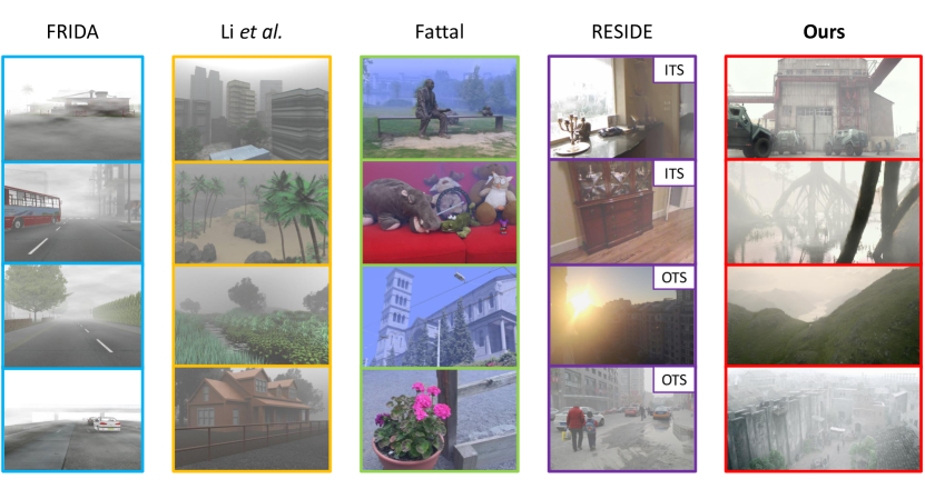
Figure 1: Visual comparison of the existing datasets including Frida [8], Li et al. [11], Fattal [12], RESIDE [7], and our proposed dataset LSFD. ITS and OTS indicate indoor training set and outdoor training set respectively.

In this paper, we argue that a large-scale high-quality and realistic dataset is the bottleneck for current dehazing algorithm. Especially, accurate and physically-valid ground truth is crucial for effectively training a dehazing method.

First, most datasets are too small for modern data driven methods. Some of the datasets (e.g.,  [6],  [8] and  [11]) contain only dozens of samples, which are not enough for learning-based methods. Second, the quality of the depth of existing outdoor datasets is undesirable. For example, [7] is a large-scale indoor and outdoor dehazing dataset. The synthetic haze is rendered on indoor scenes, which differs from the real-world scenarios. In addition, the outdoor subset of [7] applies monocular depth estimation to obtain the depth. However, the estimated depth is neither physically valid nor accurate, causing the rendered hazy images to appear as unrealistic. Lastly, the existing outdoor datasets are unrealistic. As proved by our benchmark, training on unrealistic dataset limits the generalizability of data-driven models drastically.

We tackle the aforementioned problems using High-Definition (HD) videos. Based on the physics modeling in Eq. 1, we propose a large, high quality, highly diversified dataset. To create this dataset, we select 2000 high quality ground-truth images from 3D movies with 1920 $\times$ 1080 resolution. The images are captured by high-end cameras where the color, exposure, and sensor noise are optimized. The 2000 background images are from 22 different movies with 40 hours in total to ensure their diversity. More importantly, all those movies are captured by multi-view stereo cameras, so that we can obtain high quality depth using multi-view stereo enables us to render the high quality and physics realistic hazy images. Fig. 1 shows some examples and comparisons with existing datasets. Details of the dataset creation are described in Sec. 3.

Based on it, this paper proposes a systematic and detailed benchmark using the proposed dataset and existing datasets. We believe this work will enable more exciting and novel topics in dehazing.

Table 1: Comparison of the proposed dataset with existing dehazing datasets. Our dataset contains the most diverse and accurate depth.

	Indoor	Outdoor	Background	Diversity	Haze effect	Depth accuracy	Resolution
Fattal [6]	4	8	Real	Low	Using depth	High	624 $\times$ 416
FRIDA [8]	-	480	Synthetic	Low	Using depth	High	640 $\times$ 480
Li et al. [11]	-	5	Synthetic	Low	Ray tracing	-	640 $\times$ 480
O-Haze [13]	-	45	Real	High	Using depth	High	3200 $\times$ 2900
RESIDE-ITS [7]	1399	-	Real	Low	Using depth	High	620 $\times$ 460
RESIDE-OTS [7]	-	2061	Real	High	Using depth	Low	549 $\times$ 718
Foggy-CityScape [14]	-	5000	Real	Low	Using depth	High	1280 $\times$ 960
Foggy-Driving  [14]	-	101	Real	Low	Using depth	High	640 $\times$ 480
Ours	-	2000	Real	High	Using depth	High	1920 $\times$ 1080

The main contributions of this paper are summarized as:

• We create a large-scale outdoor dehazing dataset of real scenes.

• The proposed dataset are developed based on high-definition (HD) images, rendered with physically-valid haze.

• We provide a systematical benchmark for state of the art dehazing methods on both RESIDE [7] dataset and the proposed dataset.

2 Related Work

Haze removal from a single image has attracted wide attention. While early research works on dehazing using multiple images (e.g. [15, 16]) or additional information from other sources (e.g. [17, 18]), modern methods work on single image using data-driven methods [19, 20, 21, 22, 23]. A comprehensive survey for dehazing can be found in [11]. In this work, we only focus on single image dehazing.

Dehazing datasets Quantitative evaluation and supervised learning for dehazing require the hazy image and the pixel-wise corresponding clear image as a reference. These pairs are difficult to capture in real as it is usually impossible to control the outdoor environments. Alternatively, the most common approach is to render haze on clean images with its depth using Eq. 1 [6, 7, 8]. An exception is the dataset of Li et al. [11] that applies physics-based rendering (i.e. ray tracing) [24] to generate the haze effect on synthetic scenes. Fattal [6] renders from real images and their depth maps. FRIDA [8] dataset focuses on driving scenarios and uses synthetic road backgrounds from graphics models. The datasets are small and are not suitable for learning-based methods. Recently, [14] introduces a foggy Cityscapes dataset using images from the Cityscapes dataset [25]. However, the depth map quality in Cityscapes is poor in terms of considering is as haze transmission ground truth. Therefore the hazy images rendered from them are not satisfying. In addition, the Foggy-Driving dataset only contains 101 samples with varying image size. This dataset is only suitable for benchmarking dehazing methods. [13] introduces a small set of 45 fine-crafted hazy images, which are usually served well in evaluating dehazing methods rather than providing a training option for learning-based methods. [7] proposes a general dehazing dataset named RESIDE. Its indoor training set (ITS) is built on existing indoor RBGD datasets NYUv2 [26] and Middleburry stereo [27]. The outdoor training set (OTS) collects real outdoor images with their depth estimated using learning-based single image 2D to 3D estimation [28]. The accuracy of learning-based depth is still not satisfying because it is much poorer than physically measured depths. However, the physically measuring is impractical currently due to the limitation of technical facilities. Other kinds of datasets like subjective evaluation datasets and task-driven datasets are not discussed here.

Single image dehazing methods Early works on single image dehazing are mostly prior based methods and do not require training data [5, 29, 30, 31, 32, 33, 34, 35, 36]. These works propose different priors in estimating the transmission map and the air light and then a clean image can be recovered by reversing the hazy image model in Eq. 1. Among the works, [37] observes an interesting phenomenon of outdoor natural scenes with clear visibility and formulate as dark channel prior (DCP), which becomes one of the most successful priors to dehaze. Unlike the previous local priors, [38] develops a non-local prior which relies on the assumption that colors of a haze-free image form tight clusters in RGB space. Convolution neural network (CNN) based methods gain increasing popularity in recent years [39, 40, 41, 42, 43, 44, 45, 19, 20, 21, 22, 23]. Methods [21, 22] incorporate traditional dehazing priors and color processing operations into the deep network. Generative adversarial network (GAN) based dehazing methods have been proposed in [42, 19]. The recent state-of-the-art method [44, 46, 47, 48, 49, 50, 51] applies a novel attention-based multi-scale estimation on a grid network.

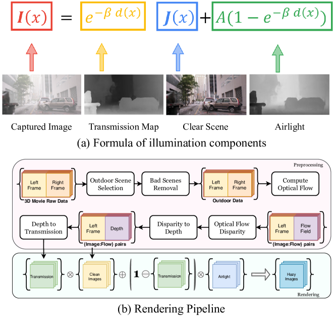
Figure 2: An illustration of the haze image visibility model (a) and the proposed dataset generation pipeline (b). The data rendering pipeline shows all the key stages to transform a raw 3D movie video into a sequence of image-depth pairs. With a series of high-resolution images and their paired depth maps, we create the hazy image data based on the visibility model described in (a).

3 Large-scale Real Outdoor Dataset

In this section, we introduce the details of our large-scale fine-depth outdoor dataset LSFD. To elaborate, we first introduce the overall features of the dataset in Sect. 3.1, followed by the motivation to choose high-quality movies as our dataset source. Finally, we describe the details of the 3D movie pre-process in Sect. 3.3 and the haze rendering process in Sect. 3.4.

3.1 Dataset Overview

Table 1 shows the key specifications of our dataset and comparison with existing datasets. The proposed dehazing dataset contains a total of 10000 images, of which 8000 images are for training set and the rest 2000 images belong to the test set. The hazy images are rendered on 2000 high-quality clean images, extracted from a series of High-Definition (HD) 3D movies. In order to diversify the background scenes, we extract more than 100 key stereo frame pairs from each of the 22 movies, resulting more than 2400 different background scenes. After our pre-process pipeline, we kept final 2000 high-quality background scenes. For each background scene, we render 5 hazy images on each clean background frame with various haze densities. For the training set, each sample contains four items including the rendered hazy image $\mathbf{I}$, the transmission map $\mathbf{T}$, the atmospheric light value $\mathbf{A}$ and the corresponding clean background image $\mathbf{J}$.

3.2 Outdoor Image with Fine Depth

Sakaridis [14] dataset focuses specifically on semantic scene understanding for the driving scenes, which is not listed. From Table 1, we can see that early datasets contain very limited number of samples, which are not suitable for modern data-driven methods. Existing large-scale outdoor dehazing dataset, i.e.  the "RESIDE-SOTS" dataset  [7], however is rendered based on the monocular depth estimation method [28]. Monocular depth estimation is not physically valid in terms of providing ground truth for haze rendering and hence the depth results are not always reliable throughout different outdoor scenes, particularly those depth estimation methods, which they use, does not perform reliably at many texture-less and ambiguous areas. In contrast we utilizes multi-view stereo [52], which is based on geometric measures and can provide robust and accurate outdoor depth.

Other than quality of depth and the absolute number of training samples, a good dataset should have a good coverage of diversified real scenes. So as to enable general applicability and avoid dataset bias. To this end, we find 3D movies provide the largest known source, presenting the possibility of capturing millions of outdoor scenes. Modern high-quality 3D movies are usually captured by top-notch stereo cameras and feature diverse and dynamic environments that range from human-centric imagery (such as Hollywood films) to nature scenes with landscapes and animals in scientific documentaries. To that end, we select a diverse set of 22 recent 3D movies with stereo image-pairs available.

(a)

(b)

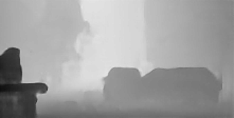
(c)

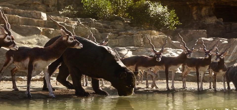
(d)

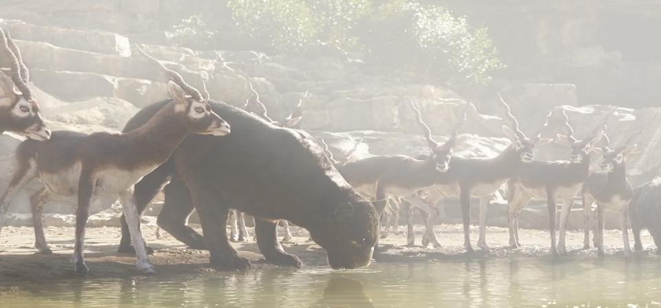
(e)

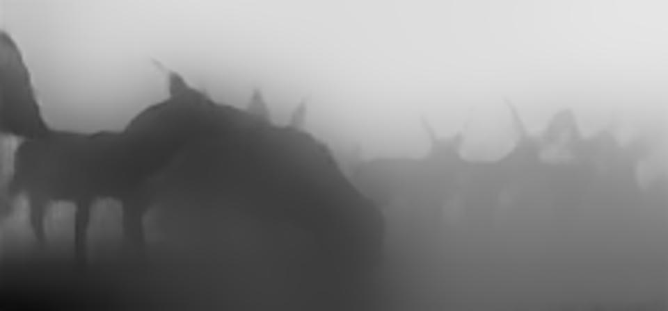
(f)

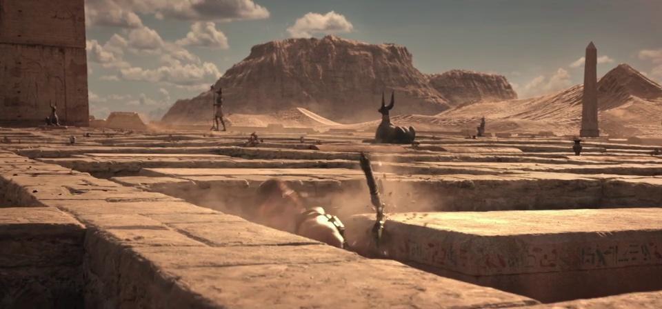
(a) Clean Background (Ground-truth)

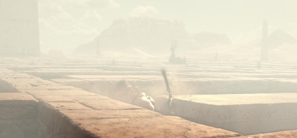
(b) Rendered Hazy Image

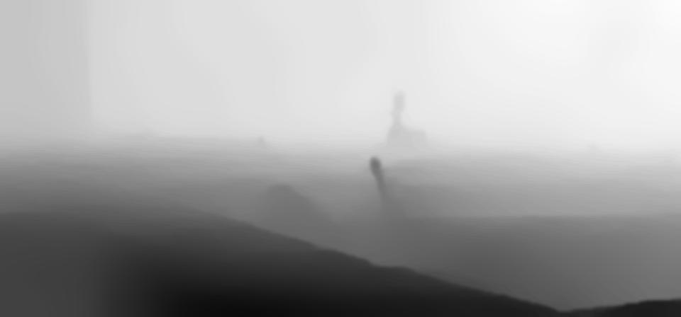
(c) Depth Map

Figure 3: Examples of the proposed dataset, while the clear images are stereo pairs, only one is shown in the figure.

3.3 High Quality Depth using 3D HD Movies

Outdoor Scene Selection In order to obtain rich and diverse outdoor scenes, we carefully select 22 3D-movies. In a typical 2-hour movie, the video may contain up to hundreds of different indoor and outdoor scenes. In order to obtain consecutive frames in the same scene, we split the long video into individual segments separated by scene transitions. For automatic scene selection, we use scene detection [53] to split each movie into independent scene. For each segment, we extract up to 2 frames (image pairs) as clean background images. These two frames are selected from the first and the last of the segment respectively to ensure larget displacement. All the extracted frames form the image set $S_{0}$. Note that $S_{0}$ contains both indoor and outdoor scenes. We separate the indoor and outdoor scenes using semantic segmentation. We use state-of-the-art method [54]. From the result, we only select the images with typical outdoor objects including grassland, road, building, landscape, etc. Lastly, not all the images from $S_{1}$ are useful for haze rendering because of various reasons. For example, some of the scenes are recorded under foggy, hazy, or smoky conditions. Others may contain strong motion blur or de-focus blur, low-light or dark images, texture-less images, foggy or hazy backgrounds, science-fiction or other style unnatural scenes, etc. We therefore do a manual check and remove the flaw samples. The final set is denoted as $S_{2}$.

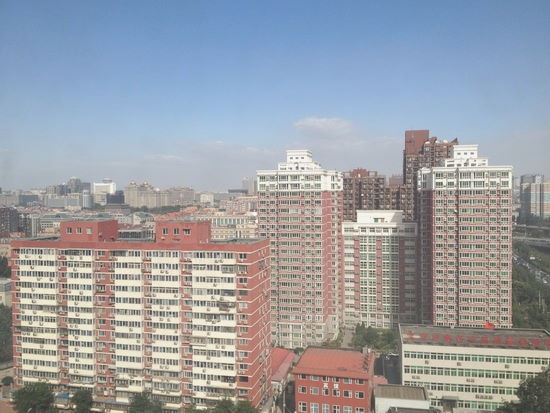
(a) Hazy Image [7]

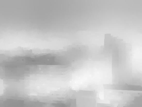
(b) Depth [7]

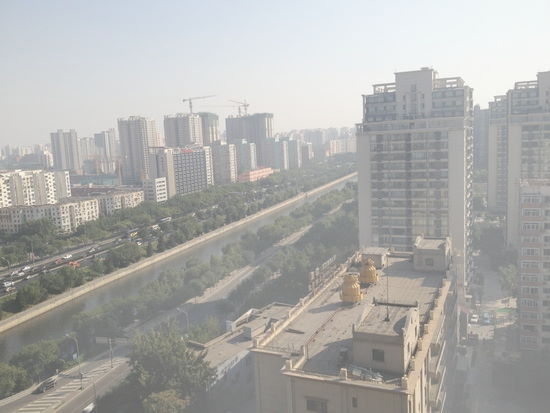
(c) Hazy Image [7]

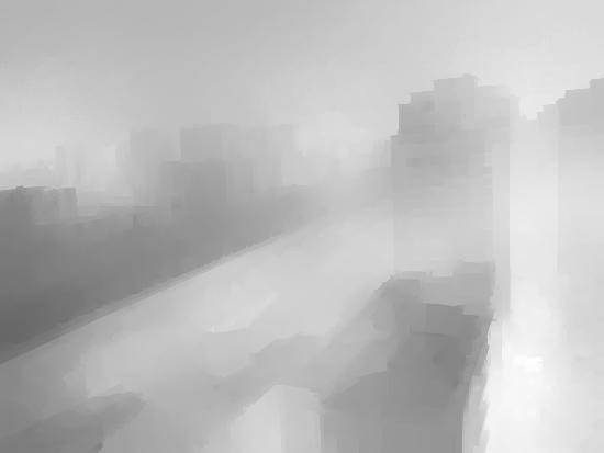
(d) Depth [7]

(e) Our Hazy Image

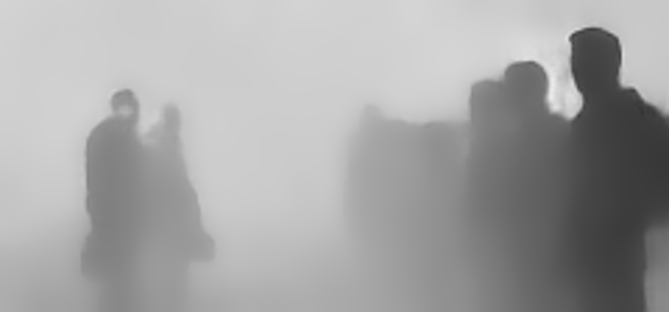
(f) Our Depth

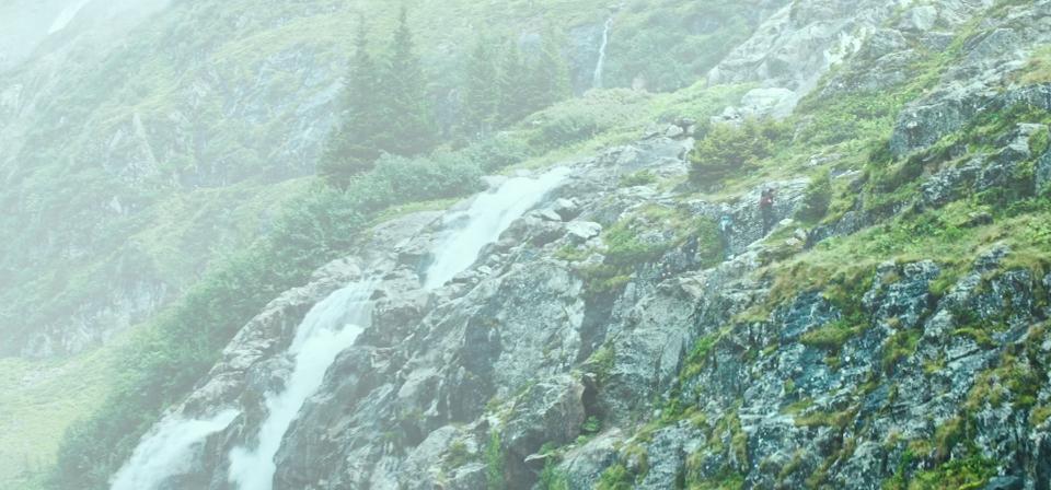
(g) Our Hazy Image

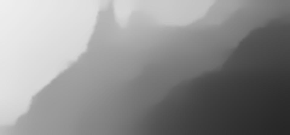
(h) Our Depth

Figure 4: Hazy images and corresponding depth maps of Comparison on rendering and depth map with RESIDE-OTS [7]. RESIDE-OTS uses empirical monocular depth estimation  [28]. The unreliable depth also results in unrealistic haze rendering. In contrast, our depth is based on physical measurement and thus reliable; and leads to realistic haze rendering.

High-Quality Depth Map As argued, a major advantage of our proposed dataset is the high-quality depth. In detail, we ensure that our depth maps are strictly from real measurements. Notice that some of the 3D movies are actually created by synthetic depth, those movie cannot provide reliable depth following the physics model. Therefore, we only use the images which are captured by real stereo cameras.

In practice, we solve some technical challenges. First, we notice that there are information loss such as camera focal lengths, camera baselines, and intrinsic parameters. Second, while most stereo algorithms assume transition between cameras, which generate only positive disparities, 3D movie data may have negative disparities depending on the camera positioning. To solve it, we use optical flow estimation PWCNet [52] instead of applying stereo algorithms. We use only the horizontal part of the estimate flow and regard it as disparity as shown in Fig. 2(b) (Middle Row). Lastly, PWCNet [52] produces flow maps at a quarter of the natural resolution. We apply FGI [55] algorithm to up-sample the flow to its original resolution. The benefit of FGI it that it is content aware and can provide sharp and precise boundaries. After obtaining the disparities, the depth is inversely proportional to it. Fig. 4 is a comparison of the depth with RESIDE dataset. As can-be seen, while RESIDE depth can be incorrect and blurry, our depth is more reliable and sharp.

Although 3D movies provide stereo image pairs for every frame, the movie data comes with its own issues as well. First, some 3D films are shot with monocular cameras and the stereo effects are manually added by post-processing. In this case, we do not include those movies in our dataset as we only select movies that were shot using physical stereo cameras. Second, we only select high-definition movies in Blu-ray storage format, which allow us to extract high-resolution image pairs. In addition, camera focal lengths, stereo camera baselines, and camera intrinsic parameters are usually unknown and these parameters vary from one movie to another. It is difficult to directly compute the stereo disparity solely from the image pairs using the state-of-the-art stereo estimation algorithms. In addition, most of the stereo algorithms are designed and trained to estimate disparity in positive ranges only. However, the 3D movie data may contain negative disparity values because of the camera position settings in the stereo rig configuration. Instead of applying stereo algorithms, we apply the state-of-the-art optical flow estimation method PWCNet [52] to handle the positive and negative disparity values. We only retain the horizontal component of the flow field as the disparity as shown in Fig. 2(b) (Middle Row). As the depth is inversely proportional to the horizontal disparity computed in last step, we convert the disparity map to depth map for each image as shown in Fig. 3 (a) and (c).

Depth Map Refinement The PWCNet [52] produces flow fields in a quarter of the original image size. A bi-linear up-sampling post-processing is usually used to up-sample the flow fields to the full size. In our case, the bi-linear up-sampling usually makes the object’s boundary blurry, which also leads to halo effect on the rendered object’s boundary. To that end, we apply FGI [55] algorithm to up-sample the flow fields based on the boundary, contours, and edges of the input image shown in Fig. 4. From the figure, We can observe that the depth discontinuities are more aligned with the actual objects’ boundaries in the input images. Hence, the halo effects of the FGI up-sampled results are significantly reduced compared with depth maps from RESIDE-$\beta$ dataset.

3.4 Hazy Image Rendering

Attenuation

Our rendering follows the haze model We follow Eq. 1 to render haze using depth. Algorithm 1 describes the details. We also apply refinement to improve from Eq. 1. Background blurriness is a function related to the depth due to Rayleigh scattering, following McCartney[56], we apply Gaussian smooth with depth-aware kernel to the haze-free images. To diversify haze density ($\beta$ in Eq. 1), we synthesize 5 hazy images using different $\beta$ which is randomly sampled from a uniform distribution in the interval of $[1.0,2.5]$.

Atmospheric Light

The atmospheric light needs to be consistent with the environment lighting and tone of the haze-free image. We use classic MaxRGB illumination estimation[57] to determine $\mathbf{A}$:

$$\centering\mathbf{A}_{M}=\max_{\mathbf{x}\in{\mathbf{\Omega}}}{M(\mathbf{x})},M\in\{R,G,B\},\@add@centering$$ (2)

where $R,G,B$ indicate red, green, blue channel of a haze-free image. $\mathbf{\Omega}$ means all pixels of $\mathbf{I}$.

Splitting

In total, we have 2000 haze-free images which now generates in total 10,000 hazy images. To training and testing split, the training set contains 8000 hazy images (1600 haze-free) and the test set contains 2000 hazy images (400 haze-free). Examples are shown in Fig. 3.

Algorithm 1 Proposed Haze Rendering Algorithm

1:Input: Clean Image $\mathbf{J}$ and its depth map $\mathbf{d}$

2:$\mathbf{J}_{blur}(\mathbf{x})=\mathsf{imgaussfilt}(\mathbf{J}(\mathbf{x}),\mathbf{\sigma}(\mathbf{x}))$. The kernel varies according to depth: $\mathbf{\sigma}(\mathbf{x})=1.5\mathbf{d}(\mathbf{x})$.

3:Obtain Transmission $\mathbf{T}=\exp^{-\beta\mathbf{d}},\beta\sim\textit{U}(1.0,2.5)$.

4:Obtain global atmospheric light $\mathbf{A}$ based on Eq. 2.

5:Output: Hazy Image $\mathbf{I}=\mathbf{T}_{blur}\mathbf{J}+(1-\mathbf{T}_{blur})\mathbf{A}$.

Table 2: The quantitative results of the state of the art methods tested on the proposed dataset LSFD test set as well as on RESIDE-SOTS dataset. For CNN-based methods, we use the pre-trained weights provided by the authors, indicated as ’official’. For those methods without official weights, we train them with RESIDE-OTS and LSFD and mark the training sets after each method respectively.

Methods	LSFD				RESIDE-SOTS		Time (s)	Platform
	PSNR	PSNR-STD	SSIM	SSIM-STD	PSNR	SSIM
BCCR [29]	17.91	2.27	0.729	0.083	16.88	0.7913	3.85	CPU
DCP [37]	19.56	2.38	0.761	0.069	16.62	0.8179	1.62	CPU
CAP [31]	14.64	3.79	0.715	0.111	19.05	0.8364	0.95	CPU
Non-Local [38]	18.06	2.78	0.727	0.079	17.29	0.7489	9.89	CPU
GRM [32]	17.48	2.27	0.682	0.083	18.86	0.8553	83.96	CPU
MS-CNN(official) [20]	10.85	3.17	0.687	0.110	17.57	0.8102	2.60	GPU
AODnet(official) [41]	12.42	2.99	0.639	0.099	19.06	0.8504	0.65	GPU
DehazeNet(official) [40]	19.76	-	0.788	-	21.14	0.8472	2.51	GPU
DCPDN(official) [23]	15.38	-	0.660	-	-	-	-	-
GridDehazeNet(official) [44]	12.37	3.38	0.659	0.120	30.86	0.9819	0.26	GPU
EPDN(official) [19]	14.44	3.26	0.797	0.081	25.06	0.9232	0.80	GPU
4K Dehazing(official) [58]	17.31	3.01	0.727	0.090	18.39	0.882	0.03	GPU
PSD(official) [59]	10.79	2.53	0.619	0.113	15.15	0.737	0.93	GPU
MSBDN(official) [60]	25.99	2.02	0.870	0.044	33.79	0.9835	0.11	GPU
FFA-Net(official) [61]	25.37	3.25	0.941	0.074	33.57	0.9840	0.23	GPU
DF2M-Net [62] (RESIDE)	24.66	4.23	0.918	0.097	34.29	0.9844	0.07	GPU
DF2M-Net [62] (LSFD)	28.49	3.75	0.943	0.083	29.88	0.9376	0.07	GPU

4 Benchmark

Experiment Setup

We provide systematical benchmark on 16 representative conventional methods and data-driven methods. The traditional methods include Boundary Constrained Context Regularization (BCCR) [29], Color Attenuation Prior (CAP) [31], Dark-Channel Prior (DCP) [37], Artifact Suppression via Gradient Residual Minimization (GRM) [32], and Non-local Image Dehazing (non-local) [38]. These methods do not require training process and therefore we directly run the methods on the dedicated test sets respectively. Data-driven methods include DehazeNet [40], Multi-scale CNN (MSCNN) [20], All-in-One Dehazing (AODNet) [41], Densely Connected Pyramid Dehazing Network (DCPDN) [23], grid [44], Enhanced Pix2pix Dehazing Network (EPDN) [19], Multi-Scale Boosted Dehazing Network with Dense Feature Fusion (MSBDN) [60], DF2M-Net [62], 4K Dehazing [58], FFA-Net [61] and PSD [59].

We use PSNR [63] and SSIM [64] metrics to evaluate all the methods. The conventional methods are directly applied on the proposed test set. For CNN-based methods, we directly use the weights provided by the author to test on the proposed datasets if available. For those methods which do not lease any pre-trained weights, we particularly train the methods on the training sets and evaluate them on the test set.

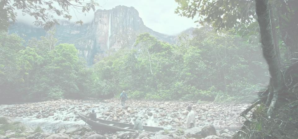
(a) Input

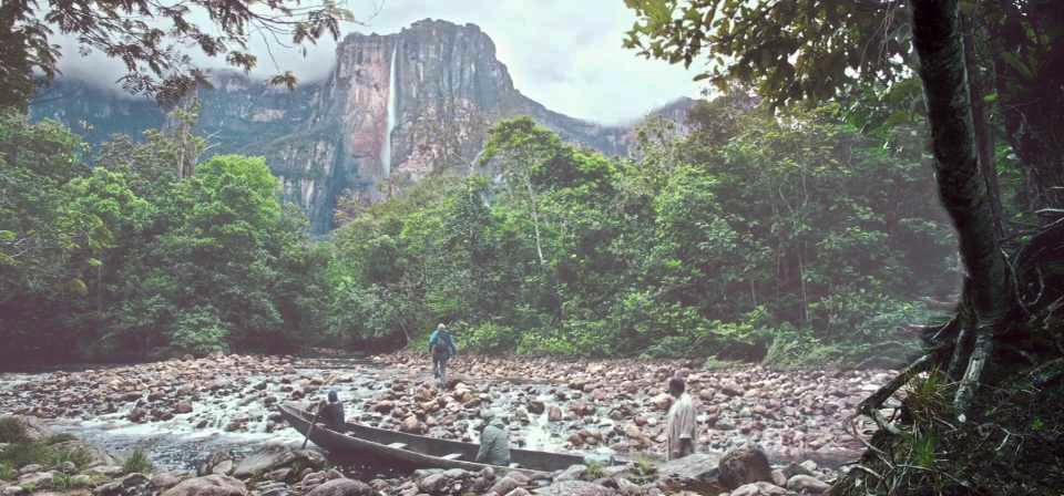
(b) CAP [31]

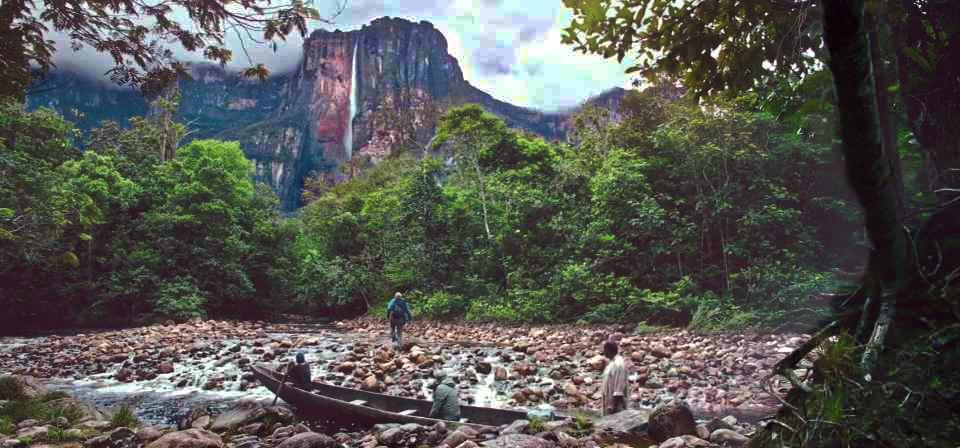
(c) DCP [37]

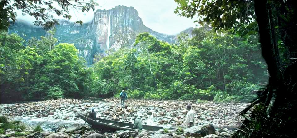
(d) Non-Local [38]

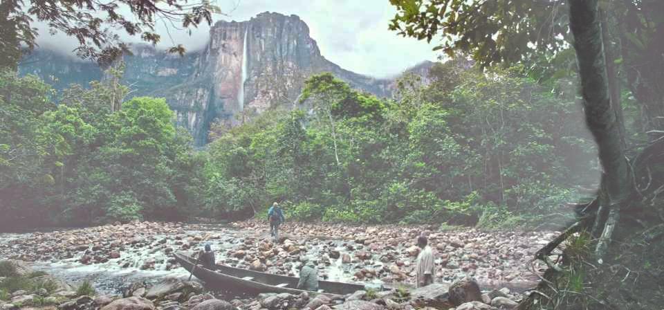
(e) MS-CNN [20]

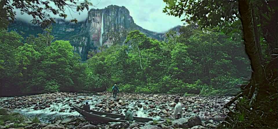
(f) AODNet [41]

(g) GridDehazeNet [44]

(h) MSDBN[31]

(i) FFA-Net [31]

(j) DehazeNet [40]

(k) DCPDN [23]

(l) GT

Figure 5: Qualitative results on the proposed LSFD dataset.

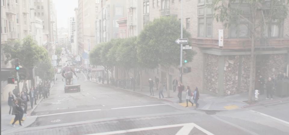
(a) Input

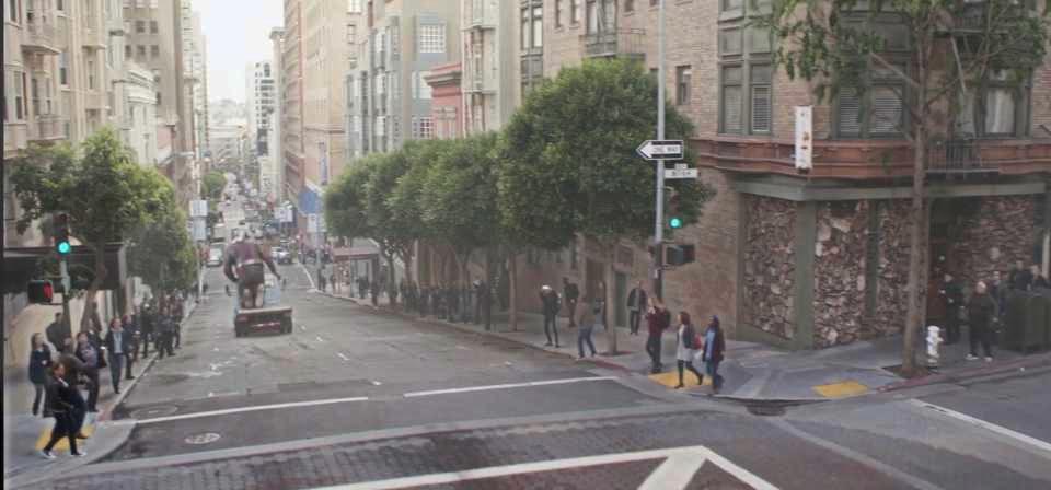
(b) CAP [31]

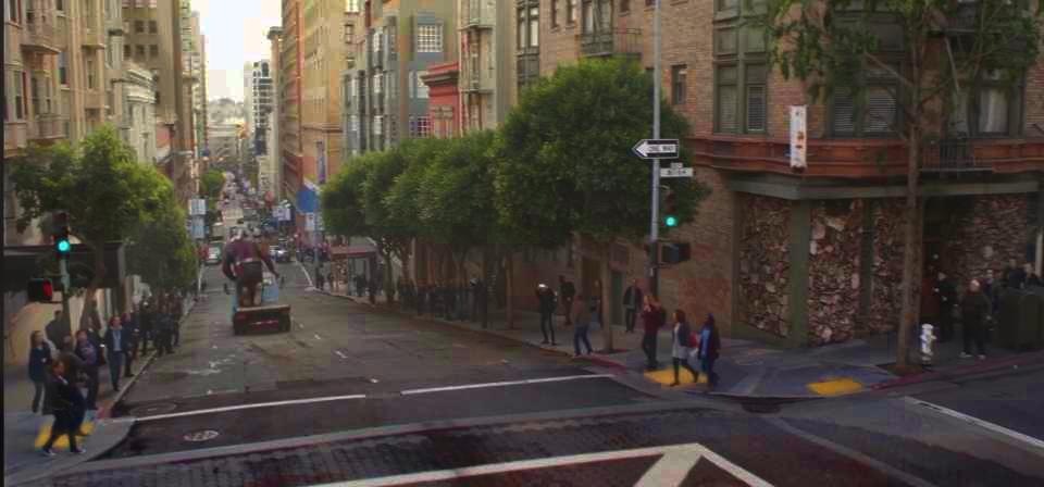
(c) DCP [37]

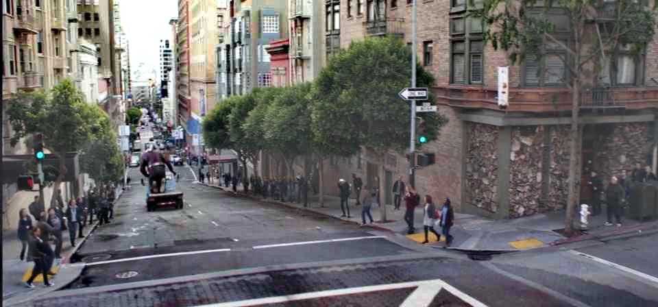
(d) Non-Local [38]

(e) MS-CNN [20]

(f) AODNet [41]

(g) GridDehazeNet [44]

(h) DehazeNet [40]

(i) FFA-Net [20]

(j) MSBDN [20]

(k) DCPDN [23]

(l) GT

Figure 6: Results comparison on the proposed LSFD dataset.

4.1 Results and Analysis

Overall performance

First of all, we provide an overview of the performance of all the selected dehazing algorithms in Table 2. For reference, we also benchmark the methods on RESIDE-$\beta$ dataset. The numbers are quoted from their benchmark if available, otherwise we benchmark them if they release training and testing code. Time and platform is also provided, as extra information. From the results, we can see that the PSNR and SSIM is not as saturated as RESIDE-$\beta$, which shows that the proposed dataset it more diversified and less likely to be over-fitted. In addition, we see performance ranking on two different datasets are clearly different, which shows the significant different of two datasets, especially the quality of depth.

Analysis

To demonstrate the generalizability of the proposed dataset, we have trained recent state of the art methods DF2M-Net [62], 4K Dehazing [58] both on the proposed LSFD dataset(training set) and RESIDE-OTS [7] dataset. And we tested the trained models on another existing high-quality O-Haze [13] dataset. The quantitative results are shown in Table 3. One can observe that both of the methods trained on the proposed LSFD dataset obtain better performance evaluated on O-Haze dataset. Visual comparison is also demonstrated in the Fig. 7. More results tested on other existing dehazing datasets and real haze images can be found in the supplementary material.

Table 3: Baseline methods trained on the proposed LSFD dataset and RESIDE-OTS dataset, tested on O-Haze (NTIRE2018) dataset

Training Data	Method	PSNR	SSIM	Method	PSNR	SSIM
RESIDE-OTS	DF2M-Net [62]	14.55	0.5357	4K Dehazing [58]	15.36	0.5792
LFSD (ours)	DF2M-Net [62]	16.65	0.6380	4K Dehazing [58]	17.01	0.6836

(a)

(b)

(c)

(d)

(a) Input

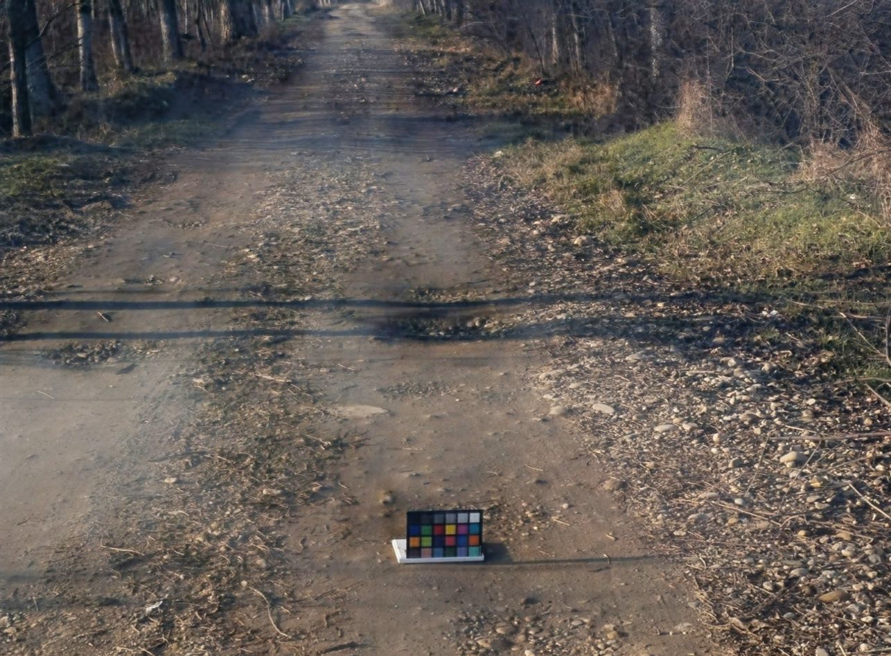
(b) DM2F (RESIDE)

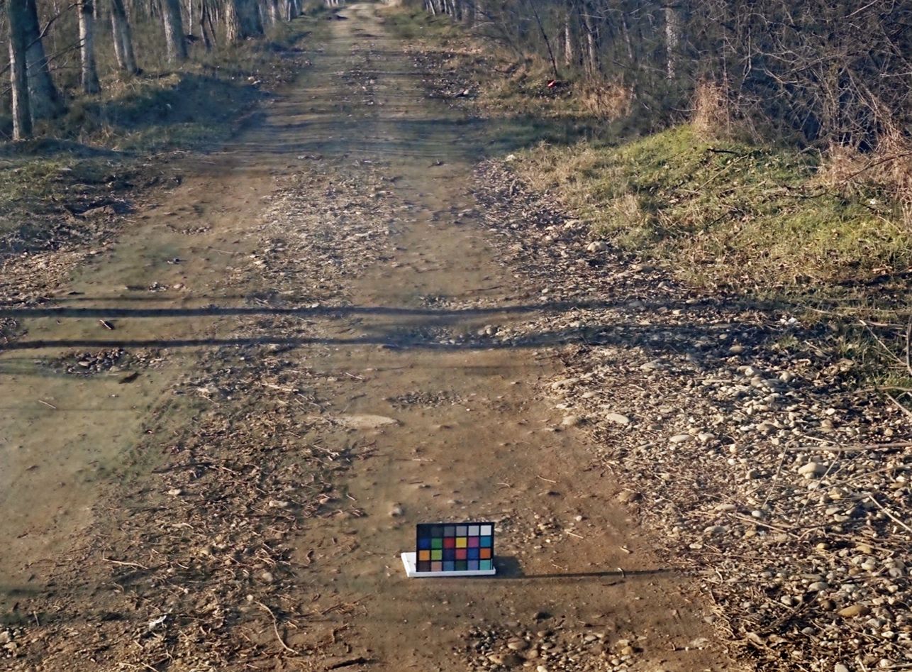
(c) DM2F (LSFD)

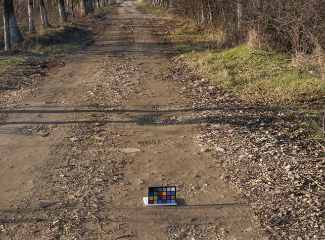
(d) Ground Truth

Figure 7: The figure shows the O-Haze test results of DM2F-Net algorithm trained on RESIDE dataset and the proposed dataset respectively.

4.2 Experimental Analysis

In Table 2, many recent CNN-based methods such as 4K Dehazing [58], PSD [59] and EPDN [19] methods do not produce convincing results compared with similar state of the art methods [62]. Moreover, these methods are even performing worse than traditional dehazing algorithms in the Table. As these methods are pre-trained on other dehazing datasets by respective authors, most of the performance drop comes from the domain gaps brought about by different datasets. Indicated in their original papers, these methods are usually pre-trained on the RESIDE-OTS dataset, the background of which is quite different from the proposed LSFD dataset. Some of the methods are quite over-fitting to the training data. Although the background images in the RESIDE-SOTS test set are different from those in the training data, then dataset generation process is actually the same, including the depth maps generation and the haze rendering. Therefore, those pre-trained methods are performing good on the RESIDE-SOTS test set, while it does perform badly in other datasets due to clear domain gap.

Data distribution comparison with RESIDE In Fig. 8, we have illustrated more city skyscraper examples from the proposed LSFD dataset. These cityscape scenes as well as more diverse modern city views are quite prominent in the proposed dataset.

5 Limitation

The limitation of the proposed dataset can be scrutinized from the data rendering process. As the proposed haze/depth rendering pipeline relies on the optical flow pre-trained model, in theory, the obtained depth maps do not have perfect accuracy compared against physical measurements. However, current technical facilities does not support accurate and dense outdoor depth measurements. In addition, the atmospheric light estimation is also following the widely used MaxRGB illumination algorithm, which could not always handle extreme cases well.

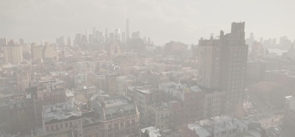
(a)

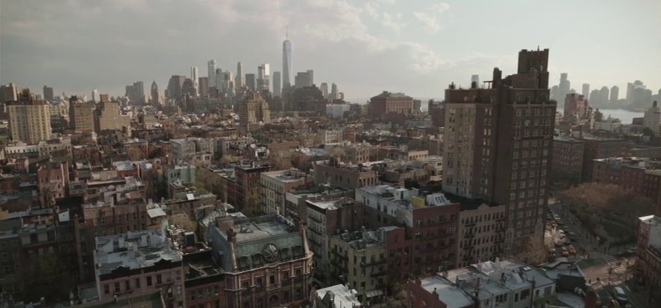
(b)

(c)

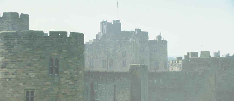
(d)

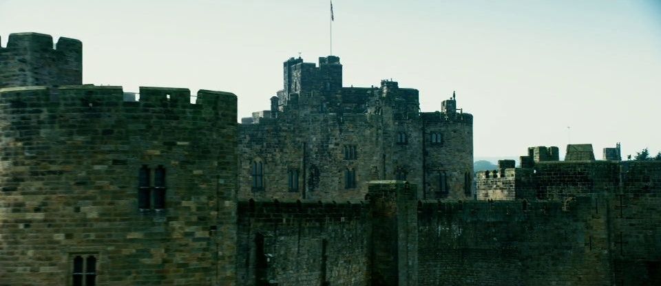
(e)

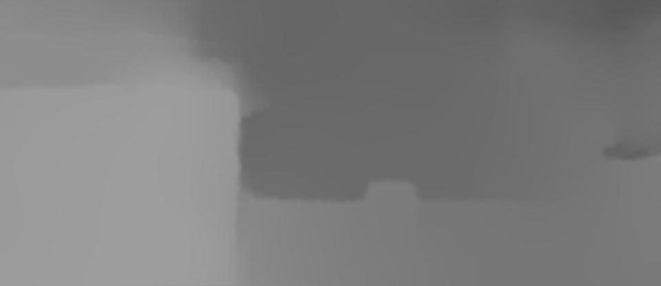
(f)

Figure 8: Example images of outdoor buildings or skyscrapers in the proposed dataset.

6 Conclusion

We propose a new, large-scale, high-definition and diverse dehazing dataset, which contains real outdoor scenes. We select high quality stereo images of real outdoor scenes and render haze on them using depth from stereo pair. Comparing with previous datasets, our dataset is more realistic due to our high-quality depth. We demonstrate that using this proposed dataset greatly improves the dehazing performance on real scenes. Our dataset is a good complement to existing dehazing datasets and our method provides a practical dehazing solution that is both efficient and effective. We will make the resources available for further dehazing research.

References

- [1] B. T. Nalla, T. Sharma, N. K. Verma, and S. R. Sahoo. Image dehazing for object recognition using faster rcnn. In International Joint Conference on Neural Networks (IJCNN), 2018.
- [2] Christos Sakaridis, Dengxin Dai, and Luc Van Gool. Semantic foggy scene understanding with synthetic data. International Journal of Computer Vision, 126(9):973–992, Sep 2018.
- [3] Sang-Kyoon Kim, Kyoung-Ho Choi, and Soon-Young Park. A framework for object detection by haze removal. Journal of the Institute of Electronics and Information Engineers, 51:168–176, 05 2014.
- [4] Gun Li, Zi-yang Wang, Jian Luo, Xin Chen, and Hou-biao Li. Spatio-context-based target tracking with adaptive multi-feature fusion for real-world hazy scenes. Cognitive Computation, 10, 08 2018.
- [5] Robby T Tan. Visibility in bad weather from a single image. In IEEE Conference on Computer Vision and Pattern Recognition, 2008.
- [6] Raanan Fattal. Dehazing using color-lines. ACM Transactions on Graphics, 34(1):13:1–13:14, 2014.
- [7] Boyi Li, Wenqi Ren, Dengpan Fu, Dacheng Tao, Dan Feng, Wenjun Zeng, and Zhangyang Wang. Benchmarking single-image dehazing and beyond. IEEE Transactions on Image Processing, 28(1):492–505, 2019.
- [8] J-P Tarel, Nicolas Hautière, Laurent Caraffa, Aurélien Cord, Houssam Halmaoui, and Dominique Gruyer. Vision enhancement in homogeneous and heterogeneous fog. IEEE Intelligent Transportation Systems Magazine, 4(2):6–20, 2012.
- [9] Harald Koschmieder. Theorie der horizontalen Sichtweite: Kontrast und Sichtweite. Keim & Nemnich, 1925.
- [10] Julia Lüthen, Julian Wörmann, Martin Kleinsteuber, and Johannes Steurer. A rgb/nir data set for evaluating dehazing algorithms. In IQSP, 2017.
- [11] Yu Li, Shaodi You, Michael S Brown, and Robby T Tan. Haze visibility enhancement: A survey and quantitative benchmarking. Computer Vision and Image Understanding, 165:1–16, 2017.
- [12] Raanan Fattal. Single image dehazing. ACM Transactions on Graphics, 27(3):72, 2008.
- [13] Codruta O. Ancuti, Cosmin Ancuti, Radu Timofte, and Christophe De Vleeschouwer. O-haze: a dehazing benchmark with real hazy and haze-free outdoor images. In IEEE Conference on Computer Vision and Pattern Recognition, NTIRE Workshop, NTIRE CVPR’18, 2018.
- [14] Christos Sakaridis, Dengxin Dai, and Luc Van Gool. Semantic foggy scene understanding with synthetic data. International Journal of Computer Vision, 126(9):973–992, 2018.
- [15] Zhuwen Li, Ping Tan, Robby T. Tan, Steven Zhiying Zhou, and Loong-Fah Cheong. Simultaneous video defogging and stereo reconstruction. In IEEE Conference on Computer Vision and Pattern Recognition, 2015.
- [16] Srinivasa G. Narasimhan and Shree K. Nayar. Contrast restoration of weather degraded images. IEEE Transactions on Pattern Analysis and Machine Intelligence, 25(6):713–724, 2003.
- [17] Johannes Kopf, Boris Neubert, Billy Chen, Michael F. Cohen, Daniel Cohen-Or, Oliver Deussen, Matt Uyttendaele, and Dani Lischinski. Deep photo: Model-based photograph enhancement and viewing. ACM Transactions on Graphics, 27(5):116:1–116:10, 2008.
- [18] Yoav Y Schechner, Srinivasa G Narasimhan, and Shree K Nayar. Instant dehazing of images using polarization. In IEEE Conference on Computer Vision and Pattern Recognition, 2001.
- [19] Yanyun Qu, Yizi Chen, Jingying Huang, and Yuan Xie. Enhanced pix2pix dehazing network. In IEEE Conference on Computer Vision and Pattern Recognition, 2019.
- [20] Wenqi Ren, Si Liu, Hua Zhang, Jinshan Pan, Xiaochun Cao, and Ming-Hsuan Yang. Single image dehazing via multi-scale convolutional neural networks. In European Conference on Computer Vision, 2016.
- [21] Wenqi Ren, Lin Ma, Jiawei Zhang, Jinshan Pan, Xiaochun Cao, Wei Liu, and Ming-Hsuan Yang. Gated fusion network for single image dehazing. In IEEE Conference on Computer Vision and Pattern Recognition, 2018.
- [22] Dong Yang and Jian Sun. Proximal dehaze-net: a prior learning-based deep network for single image dehazing. In European Conference on Computer Vision, 2018.
- [23] He Zhang and Vishal M Patel. Densely connected pyramid dehazing network. In IEEE Conference on Computer Vision and Pattern Recognition, 2018.
- [24] Matt Pharr and Greg Humphreys. Physically based rendering: From theory to implementation. Morgan Kaufmann, 2010.
- [25] Marius Cordts, Mohamed Omran, Sebastian Ramos, Timo Rehfeld, Markus Enzweiler, Rodrigo Benenson, Uwe Franke, Stefan Roth, and Bernt Schiele. The cityscapes dataset for semantic urban scene understanding. In IEEE Conference on Computer Vision and Pattern Recognition, 2016.
- [26] Nathan Silberman, Derek Hoiem, Pushmeet Kohli, and Rob Fergus. Indoor segmentation and support inference from rgbd images. In European Conference on Computer Vision, 2012.
- [27] Daniel Scharstein and Richard Szeliski. High-accuracy stereo depth maps using structured light. In IEEE Conference on Computer Vision and Pattern Recognition, 2003.
- [28] Fayao Liu, Chunhua Shen, Guosheng Lin, and Ian Reid. Learning depth from single monocular images using deep convolutional neural fields. IEEE Transactions on Pattern Analysis and Machine Intelligence, 38(10):2024–2039, 2015.
- [29] Gaofeng Meng, Ying Wang, Jiangyong Duan, Shiming Xiang, and Chunhong Pan. Efficient image dehazing with boundary constraint and contextual regularization. In IEEE International Conference on Computer Vision, 2013.
- [30] Ketan Tang, Jianchao Yang, and Jue Wang. Investigating haze-relevant features in a learning framework for image dehazing. In IEEE Conference on Computer Vision and Pattern Recognition, 2014.
- [31] Qingsong Zhu, Jiaming Mai, and Ling Shao. A fast single image haze removal algorithm using color attenuation prior. IEEE Transactions on Image Processing, 24(11):3522–3533, 2015.
- [32] Chen Chen, Minh N Do, and Jue Wang. Robust image and video dehazing with visual artifact suppression via gradient residual minimization. In European Conference on Computer Vision, 2016.
- [33] Yu Li, Fangfang Guo, Robby T Tan, and Michael S Brown. A contrast enhancement framework with jpeg artifacts suppression. In European Conference on Computer Vision. 2014.
- [34] Yu Li, Robby T Tan, and Michael S Brown. Nighttime haze removal with glow and multiple light colors. In IEEE International Conference on Computer Vision, 2015.
- [35] Jing Zhang, Yang Cao, Shuai Fang, Yu Kang, and Chang Wen Chen. Fast haze removal for nighttime image using maximum reflectance prior. In IEEE Conference on Computer Vision and Pattern Recognition, 2017.
- [36] M. Sulami, I. Glatzer, R. Fattal, and M. Werman. Automatic recovery of the atmospheric light in hazy images. In IEEE International Conference on Computational Photography, 2014.
- [37] Kaiming He, Jian Sun, and Xiaoou Tang. Single image haze removal using dark channel prior. IEEE Transactions on Pattern Analysis and Machine Intelligence, 33(12):2341–2353, 2011.
- [38] D. Berman, T. Treibitz, and S. Avidan. Non-local image dehazing. In IEEE Conference on Computer Vision and Pattern Recognition, 2016.
- [39] Adrian Galdran, Aitor Alvarez-Gila, Alessandro Bria, Javier Vazquez-Corral, and Marcelo Bertalmío. On the duality between retinex and image dehazing. In IEEE Conference on Computer Vision and Pattern Recognition, 2018.
- [40] Bolun Cai, Xiangmin Xu, Kui Jia, Chunmei Qing, and Dacheng Tao. Dehazenet: An end-to-end system for single image haze removal. IEEE Transactions on Image Processing, 25(11):5187–5198, 2016.
- [41] Boyi Li, Xiulian Peng, Zhangyang Wang, Jizheng Xu, and Dan Feng. Aod-net: All-in-one dehazing network. In IEEE International Conference on Computer Vision, 2017.
- [42] Runde Li, Jinshan Pan, Zechao Li, and Jinhui Tang. Single image dehazing via conditional generative adversarial network. In IEEE Conference on Computer Vision and Pattern Recognition, 2018.
- [43] Yunan Li, Qiguang Miao, Wanli Ouyang, Zhenxin Ma, Huijuan Fang, Chao Dong, and Yining Quan. Lap-net: Level-aware progressive network for image dehazing. In IEEE International Conference on Computer Vision, 2019.
- [44] Xiaohong Liu, Yongrui Ma, Zhihao Shi, and Jun Chen. Griddehazenet: Attention-based multi-scale network for image dehazing. In IEEE International Conference on Computer Vision, 2019.
- [45] Yang Liu, Jinshan Pan, Jimmy Ren, and Zhixun Su. Learning deep priors for image dehazing. In IEEE International Conference on Computer Vision, 2019.
- [46] Haiyan Wu, Yanyun Qu, Shaohui Lin, Jian Zhou, Ruizhi Qiao, Zhizhong Zhang, Yuan Xie, and Lizhuang Ma. Contrastive learning for compact single image dehazing. CoRR, abs/2104.09367, 2021.
- [47] Yuanjie Shao, Lerenhan Li, Wenqi Ren, Changxin Gao, and Nong Sang. Domain adaptation for image dehazing. CoRR, abs/2005.04668, 2020.
- [48] Peter Morales, Tzofi Klinghoffer, and Seung Jae Lee. Feature forwarding for efficient single image dehazing. CoRR, abs/1904.09059, 2019.
- [49] Sourya Dipta Das and Saikat Dutta. Fast deep multi-patch hierarchical network for nonhomogeneous image dehazing. CoRR, abs/2005.05999, 2020.
- [50] Yankun Yu, Huan Liu, Minghan Fu, Jun Chen, Xiyao Wang, and Keyan Wang. A two-branch neural network for non-homogeneous dehazing via ensemble learning, 2021.
- [51] Wei-Ting Chen, Hao-Yu Fang, Jian-Jiun Ding, and Sy-Yen Kuo. Pmhld: Patch map based hybrid learning dehazenet for single image haze removal. IEEE Transactions on Image Processing, 2020.
- [52] Deqing Sun, Xiaodong Yang, Ming-Yu Liu, and Jan Kautz. PWC-Net: CNNs for optical flow using pyramid, warping, and cost volume. In IEEE Conference on Computer Vision and Pattern Recognition, 2018.
- [53] pyscenedetect. https://pyscenedetect.readthedocs.io/.
- [54] Bolei Zhou, Hang Zhao, Xavier Puig, Tete Xiao, Sanja Fidler, Adela Barriuso, and Antonio Torralba. Semantic understanding of scenes through the ade20k dataset. International Journal of Computer Vision, 2018.
- [55] Yu Li, Dongbo Min, Minh N. Do, and Jiangbo Lu. Fast guided global interpolation for depth and motion. In European Conference on Computer Vision, 2016.
- [56] Earl J McCartney. Optics of the atmosphere: scattering by molecules and particles. New York, John Wiley and Sons, Inc., 1976. 421 p., 1, 1976.
- [57] Edwin Herbert Land. The retinex theory of color vision. Scientific American, 237 6:108–28, 1977.
- [58] Zhuoran Zheng, Wenqi Ren, Xiaochun Cao, Xiaobin Hu, Tao Wang, Fenglong Song, and Xiuyi Jia. Ultra-high-definition image dehazing via multi-guided bilateral learning. In IEEE Conference on Computer Vision and Pattern Recognition, 2021.
- [59] Zeyuan Chen, Yangchao Wang, Yang Yang, and Dong Liu. Psd: Principled synthetic-to-real dehazing guided by physical priors. In IEEE Conference on Computer Vision and Pattern Recognition, 2021.
- [60] Dong Hang, Pan Jinshan, Hu Zhe, Lei Xiang, Zhang Xinyi, Wang Fei, and Yang Ming-Hsuan. Multi-scale boosted dehazing network with dense feature fusion. In IEEE Conference on Computer Vision and Pattern Recognition, 2020.
- [61] Xu Qin, Zhilin Wang, Yuanchao Bai, Xiaodong Xie, and Huizhu Jia. FFA-Net: Feature fusion attention network for single image dehazing. In Proceedings of the AAAI Conference on Artificial Intelligence, 2020.
- [62] Zijun Deng, Lei Zhu, Xiaowei Hu, Chi-Wing Fu, Xuemiao Xu, Qing Zhang, Jing Qin, and Pheng-Ann Heng. Deep multi-model fusion for single-image dehazing. In IEEE International Conference on Computer Vision, 2019.
- [63] Q. Huynh-Thu and M. Ghanbari. Scope of validity of psnr in image/video quality assessment. Electronics Letters, 44(13):800–801, 2008.
- [64] Zhou Wang, A. C. Bovik, H. R. Sheikh, and E. P. Simoncelli. Image quality assessment: from error visibility to structural similarity. IEEE Transactions on Image Processing, 13(4):600–612, 2004.