Coping with Dating Errors in Causality Estimation

Abstract

We consider the problem of estimating causal influences between observed processes from time series possibly corrupted by errors in the time variable (dating errors) which are typical in palaeoclimatology, planetary science and astrophysics. “Causality ratio” based on the Wiener – Granger causality is proposed and studied for a paradigmatic class of model systems to reveal conditions under which it correctly indicates directionality of unidirectional coupling. It is argued that in case of a priori known directionality, the causality ratio allows a characterization of dating errors and observational noise. Finally, we apply the developed approach to palaeoclimatic data and quantify the influence of solar activity on tropical Atlantic climate dynamics over the last two millennia. A stronger solar influence in the first millennium A.D. is inferred. The results also suggest a dating error of about 20 years in the solar proxy time series over the same period.

1 Introduction

Revealing cause-and-effect relationships between observed processes at various time scales is an important step in understanding many physical, biological, physiological and geophysical systems [1, 2, 3, 4, 5, 6, 7, 8]. Frequently, this issue must be addressed with rather limited knowledge about the systems under study, amounts of observational data, and dating accuracy. A general approach to detect and quantify causal couplings, i.e., to find out “who drives whom”, is the Wiener – Granger (WG) causality [2, 3]. In its simplest version, the idea is to check whether a present value of one process ($X$) can be predicted more accurately using the past of a second process ($Y$) in comparison with predictions based solely on the past of $X$. In fact, this concept generalizes a conditional (partial) cross-correlation [11] and has been followed by a number of elaborations such as information-theoretic measures [12, 3, 13, 14, 15] and various nonlinear approximations [16]. Despite some limitations and obstacles [17, 18, 19, 8], the WG causality appears quite useful in practice, allowing meaningful dynamical interpretations [10, 22] and becoming increasingly widely used in different fields, such as biomedicine [1, 5, 8] and geophysics [6].

Causal coupling estimation is also of great value in climate science, where temporal changes of climatically sensitive proxies [23] are the main source of information about past climate dynamics over long time intervals. The stalagmite YOK-I from the Yok Balum Cave in Southern Belize is especially well dated [24] and provides a high-resolution reconstruction of low-latitudinal Atlantic moisture variations [25]. Making use of solar irradiance reconstructions (e.g. [26]), one can ask “How do variations in solar activity affect regional Atlantic climate?”. Answering this question helps further delineating the time-variant processes that drive climate variations. However, this question leads directly to the main difficulty with such data: dating accuracy of the reconstructions used. Uncertainties inherent to sampling and dating methods limit our knowledge of the time instant of each proxy observation, so that temporal ordering of the observations from the two time series may be distorted uniformly or irregularly in the course of time. This makes questionable any application of the WG causality approach, which essentially requires a clear distinction between the future and the past.

In this Letter, we propose a solution with an appropriate specification of the problem setting and adaptation of the WG causality characteristics. We consider a situation where it is known in advance that the coupling between two processes underlying the observed time series is unidirectional, and the problem reduces to identifying the coupling directionality. Observational noise and dating errors may strongly affect the results of any coupling analysis. In particular, the usual cross-correlation function (CCF) is obviously insufficient since even a uniform dating error moves the location of the CCF maximum along the time axis, so that “lead – lag” information is lost. We note, however, that the WG causality approach provides two coupling characteristics corresponding to the two directions $X\to Y$ and $Y\to X$, which is a richer characterization than a single CCF value. To make the WG causality work in case of dating errors, we suggest its modification involving the definition of the causality ratio $r_{Y\to X}$ which is the ratio of maximized time-lagged truncated WG causalities in the directions $Y\to X$ and $X\to Y$. We argue that if a coupling indeed exists in the direction $Y\to X$, then under certain conditions $r_{Y\to X}>1$, i.e., the causality ratio is an indicator of the coupling directionality.

We study the conditions under which this causality ratio allows us to extract information on directionality of unidirectional coupling or, knowing the directionality, to characterize dating errors and observational noise in the analyzed time series. As for the latter task, the mentioned palaeoclimate problem is a relevant example where coupling is unidirectional from solar activity variations to regional climate (reflected in proxy reconstructions), while dating errors and observational noise in the proxy signals remain largely unknown. Here, we (i) determine the causality ratio for a class of model systems exactly, (ii) analyze statistical properties of its estimator in numerical simulations, and (iii) apply the approach to palaeoclimate data using the two records mentioned above to assess their dating accuracy and quantify the time-variant influence of solar activity on the tropical Atlantic climate. Further details of the method and additional results are given in [27].

2 Wiener – Granger causality

Let ($X(t),Y(t)$) be a bivariate random process with realizations $(x(t),y(t))$. Denote $x_{n}=x(t_{n})$, $y_{n}=y(t_{n})$, where $t_{n}=nh$, $n\in{\bf Z}$, and $h$ is the sampling interval. Consider the self-predictor $x^{ind}_{n}=E[X(t_{n})|x_{n-1},x_{n-2},\dots]$ where the expectation $E[\cdot|\cdot]$ is conditioned on the infinite past $\{x_{n-1},x_{n-2},\dots\}$. Its mean-squared error is $\sigma^{2}_{X,ind}=E[(X(t_{n})-x^{ind}_{n})^{2}]$ where the expectation is taken over all $x_{n}$ and all $\{x_{n-1},x_{n-2},\dots\}$. This error is the least over all self-predictors for $X$. The joint predictor $x^{joint}_{n}=E[X(t_{n})|x_{n-1},y_{n-1},x_{n-2},y_{n-2},\dots]$ gives the least error $\sigma^{2}_{X,joint}$ over all joint predictors. The prediction improvement (PI) $G_{Y\rightarrow X}=(\sigma^{2}_{X,ind}-\sigma^{2}_{X,joint})/\sigma^{2}_{X,ind}$ is a measure of WG causality in the direction $Y\rightarrow X$. Everything is analogous for the direction $X\rightarrow Y$.

The WG idea was first realized for stationary Gaussian processes [3]. Then, when estimating $G_{Y\rightarrow X}$ from a finite time series $\{x_{n},y_{n}\}_{n=1}^{N}$, one truncates the (conditioning) infinite pasts at finite numbers of terms $l_{X}$ and $l_{XY}$ and fits univariate and bivariate linear autoregressive models of the orders $l_{X}$ and $(l_{X},l_{XY})$ to the data via the ordinary least-squares technique. In other words, one uses the predictors $x^{ind}_{n,l_{X}}=E[X_{n}|x_{n-1},x_{n-2},\dots,x_{n-l_{X}}]$ and $x^{joint}_{n,l_{X},l_{XY}}=E[X_{n}|x_{n-1},\dots,x_{n-l_{X}},y_{n-1},\dots,y_{n-l_{XY}}]$ and gets the truncated WG causality $G^{tr}_{Y\rightarrow X}$. The latter is often a good approximation of $G_{Y\rightarrow X}$ even at small $l_{X}$ and $l_{XY}$. The model orders can be selected via the Schwarz criterion [5] and statistical significance can be checked via Fisher’s $F$-test [6].

3 Causality ratio

Consider a more general setting with the original processes $X_{0}$ and $Y_{0}$, whose observed versions $X$ and $Y$ are distorted along two lines. First, due to an amplitude noise: $X(t)=X_{0}(t)+\Xi(t)$ and $Y(t)=Y_{0}(t)+\Psi(t)$ where $\Xi(t)$ and $\Psi(t)$ are independent observational noises with variances $\sigma_{\Xi}^{2}$ and $\sigma_{\Psi}^{2}$, whose discrete time realizations $\xi_{n}$ and $\psi_{n}$ are white noises. Second, due to time uncertainty: genuine (a priori unknown) observation instants $t_{n}^{X}$ and $t_{n}^{Y}$ deviate from the supposed regular equidistant series $t_{n}=nh$: $x_{n}=x(t^{X}_{n})+\xi_{n}$ and $y_{n}=y(t^{Y}_{n})+\psi_{n}$ with $t^{X}_{n}+\delta^{X}_{n}=nh$ and $t^{Y}_{n}+\delta^{Y}_{n}=nh$, where $\delta^{X}_{n}$ and $\delta^{Y}_{n}$ stay for the time axis (i.e. dating) errors. The latter may be rapidly fluctuating or slowly varying and may be defined either as random processes or deterministic functions of time. To account for the dating errors and retain sensitivity to coupling, we use the time-lagged WG causality: namely, $G^{tr}_{Y\rightarrow X}(\Delta)$ is defined as prediction improvement of $x_{n}$ when using the segment $\{y_{n-\Delta/h},\dots,y_{n-(l_{XY}-1)-\Delta/h}\}$. Then, we suggest to determine its maximum over an interval of positive and negative time lags of some width $2\Delta_{m}$: $G^{tr,max}_{Y\rightarrow X}=\displaystyle\max_{-\Delta_{m}\leq\Delta\leq\Delta_{m}}G^{tr}_{Y\rightarrow X}(\Delta)$. Analogously we define $G^{tr,max}_{X\rightarrow Y}$. Finally, the causality ratio in the direction $Y\to X$ reads

$$r_{Y\to X}=\displaystyle\frac{G^{tr,max}_{Y\rightarrow X}}{G^{tr,max}_{X\rightarrow Y}}.$$ (1)

Obviously, $r_{X\to Y}=1/r_{Y\to X}$. The value of $\Delta_{m}$ should be chosen so as to exceed a maximal possible dating error to avoid missing the maximal PIs. If, moreover, the coupling is time-delayed, locations of the PIs maxima are shifted along the $\Delta$-axis by the value of this delay. Hence, if one expects a time delay, then the value of $\Delta_{m}$ should be selected so as to exceed the sum of the absolute values of the coupling delay and the dating error.

We conjecture that for unidirectional coupling $Y\to X$ and similar individual characteristics of the processes $X$ and $Y$, the ratio $r_{Y\to X}$ is considerably greater than unity. However, dating errors and observational noise along with estimates fluctuations due to shortness of time series may somewhat decrease $r_{Y\to X}$, which is studied below.

4 Model system

Since the value of $r_{Y\to X}$ may depend on many features of the processes under study (such as characteristic times and sampling interval) and parameters of the estimation technique (such as $l_{X}$), we need to choose a reasonably simple system and a narrow range of the parameters for which the causality ratio can be studied in detail. As such a testing system, we use coupled “relaxators” (first-order decay processes):

$$\begin{array}[]{rcl}dX_{0}/dt&=&-\alpha X_{0}(t)+kY_{0}(t)+\zeta_{X}(t),\\ dY_{0}/dt&=&-\alpha Y_{0}(t)+\zeta_{Y}(t),\end{array}$$ (4)

where $\alpha$ determines the characteristic relaxation time $\tau=1/\alpha$, $k$ is the coupling coefficient, and $\zeta_{X}$ and $\zeta_{Y}$ are independent zero-mean white noises with autocorrelation functions $E[\zeta_{X}(t_{1})\zeta_{X}(t_{2})]=E[\zeta_{Y}(t_{1})\zeta_{Y}(t_{2})]=\delta(t_{1}-t_{2})$ where $\delta$ is Dirac’s delta. Eqs. (17) represent a simple, but basic class of systems which still exhibit irregular temporal behavior and are often encountered in different fields (e.g. [30]). The squared zero-lag CCF reads here $C^{2}_{X_{0}Y_{0},0}=(\beta/4)/(1+\beta/2)$ where $\beta=k^{2}/\alpha^{2}$ is a non-dimensional coupling strength. $C^{2}_{X_{0}Y_{0},0}$ ranges from 0 (for $k=0)$ to 0.5 (for $k\to\infty$) and can be used to parameterize the coupling strength as well. The sampling rate can be conveniently characterised by the ratio $h/\tau$.

For system (17) it appears possible to confine ourselves with the orders $l_{X}=l_{XY}=l_{Y}=l_{YX}=1$. It can be argued that $G^{tr}_{Y\to X}(\Delta)$ obtained at $l_{X}=l_{XY}=1$ is close to $G^{tr}_{Y\to X}(\Delta)$ obtained at $l_{X}=\infty$ and $l_{XY}=1$, if the sampling interval $h$ is not too small (e.g. $\geq 0.2\tau$) [10]. In numerical simulations here, we also find that the results for $G^{tr}_{Y\to X}(\Delta)$ with $l_{X}=1$ are close to those obtained with $l_{X}$ selected via the Schwarz criterion (difference of the order of $1\%$). Similar arguments hold for $l_{XY}$. Then, the quantity $G^{tr}_{Y\to X}(\Delta)$ can be expressed via the autocorrelation function (ACF) $C_{XX}(h)$ and the CCF $C_{XY}(\Delta)$ and $C_{XY}(\Delta-h)$ [8, 27]. Having found ACFs and CCF analytically, we compute the time-lagged truncated WG causalities versus $\Delta$ and select their maxima to calculate the causality ratio. Such a precise analysis is performed for various coupling coefficient values, sampling intervals, observational noise and dating error levels, while statistical properties of the causality ratio estimator are investigated in numerical simulations. We check if indeed $r_{Y\rightarrow X}>1$ and assess how small $r_{Y\rightarrow X}$ can be at all. A closer attention is paid to cases with $0.1\leq C^{2}_{XY,max}\leq 0.2$ and WG causalities $0.01\leq G^{tr,max}_{Y\to X}\leq 0.03$ which are reminiscent of those often observed in climate data analysis in cases of statistically significant coupling detection (e.g. [31] and the palaeoclimate example below).

5 Exact study of possible causality ratio values

Before considering the central point of dating errors identification, it is necessary to study the case of undistorted observations $X=X_{0}$ and $Y=Y_{0}$. For the most practically interesting situations of not too sparse sampling (e.g. $h\leq 0.2\tau$), $r_{Y\to X}$ is well above unity, confidently indicating the correct coupling direction. Namely, $r_{Y\to X}=1.6$ for $h=0.2\tau$ and a moderately strong coupling of $C^{2}_{X_{0}Y_{0},0}=0.1$. For rather sparse samplings of $h\geq\tau$, the ratio $r_{Y\to X}$ gets close to unity and, hence, cannot reliably reveal coupling directionality. This is similar for any coupling strength: in particular, at $h/\tau=0.2$ the causality ratio remains almost constant ($r_{Y\to X}\approx 1.6$) in the wide range of $0<C^{2}_{XY,0}<0.3$. For stronger couplings, $r_{Y\to X}$ becomes even greater, up to $\approx 3$ at $C^{2}_{XY,0}=0.5$. Thus, if the sampling is not too sparse, $r_{Y\to X}$ correctly detects coupling directionality. More details are given in [27].

Though there can be different types of dating errors, their basic effect can be studied on a simple example where dating errors equal a constant temporal shift half the time (e.g. for an older half of a palaeoclimate record where accurate dating is more difficult) and zero otherwise. Regardless which signal is erroneously dated, only the relative dating errors matter in causality estimation. For definiteness, we introduce the dating errors only into the driving signal: $\delta^{Y}_{n}=const=\delta^{Y}$ half time (for $n=1,\dots,N/2$) and $\delta^{Y}_{n}=0$ otherwise (for $n=N/2+1,\dots,N$). The “average CCF” of such a nonstationary process $(X,Y)$ can be defined as the expectation of the sample CCF computed over the entire time span and equals an arithmetic mean of the CCFs for the two stationary halves. The usual WG causalities defined for the entire time span are expressed via such an average CCF in the same way as before. Figs. 1,a,b show that the shape of the plots for the time-lagged WG causalities and locations of their maxima change strongly when the dating error becomes comparable with the relaxation time $\tau$. Then, the “correct” $G^{tr,max}_{Y\to X}$ decreases almost two times as compared to zero dating error, while the opposite $G^{tr,max}_{X\to Y}$ decreases only 1.5 times. At that, the causality ratio becomes close to unity and may even fall down to 0.9 for the dating error greater than $\tau$. If a smaller or a larger portion of a time series suffers from a uniform dating error, then the effect of the latter on the causality ratio and the respective distortions of the plots $G^{tr}_{Y\to X}(\Delta)$ are weaker [27], in particular, they vanish if the entire time series is characterized with a uniform dating error since the causality ratio involves maximization over temporal shifts.

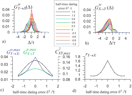
Figure 1: Causality measures depending on dating error $\delta^{Y}$ for the system (17) at $h/\tau=0.2$ and $\sigma_{\Xi}^{2}=\sigma_{\Psi}^{2}=0$, $k/\alpha$ is such that $C^{2}_{X_{0}Y_{0},0}=0.1$, $l_{X}=l_{XY}=l_{Y}=l_{YX}=1$: (a,b) truncated WG causalities versus time lag for different dating errors; (c) maximal truncated WG causalities (blue and green) and maximum CCF value (black) and (d) causality ratio versus $\delta^{Y}$.

Principally, dating errors may be distributed in a complicated manner determined both by random walk-like stochastic contribution, analytical limitations and global contribution induced by incorrect tie points as, e.g., erroneous attribution of volcanic eruption dates due to incorrect identification of individual eruptions [13]. Still, we have obtained results very similar to Fig. 1 for dating errors linearly increasing with age, even with a superimposed random-walk component whose values become of the order of $\tau$ for ages of the order of $100\tau$ as motivated by palaeoclimate applications. Thus, the described effect of the dating errors is robust, being observed just for reasonably large dating errors without any other, specific conditions.

When dating errors are present, it is natural to expect also an observational noise. Let us first show how the latter affects the causality ratio for zero dating errors. It appears that the noise $\Psi$ in the driving signal can significantly decrease $r_{Y\to X}$. Thus, at moderate $h/\tau=0.2$, $C^{2}_{X_{0}Y_{0},0}=0.1$ and $\sigma^{2}_{\Xi}=0$, the “correct” $G^{tr,max}_{Y\to X}$ decreases with $\sigma^{2}_{\Psi}$ faster than $G^{tr,max}_{X\to Y}$ so that $r_{Y\to X}$ approaches unity at $\sigma_{\Psi}^{2}/\sigma_{Y_{0}}^{2}>0.5$ (Fig. 2). However, the noise $\Xi$ in the driven signal increases $r_{Y\to X}$ apart from unity, which becomes quite visible as soon as $\sigma^{2}_{\Xi}/\sigma_{X_{0}}^{2}$ exceeds just $0.1$. To summarize, large values of $\sigma^{2}_{\Psi}/\sigma_{Y_{0}}^{2}$ ($50\%$ and greater) along with small $\sigma^{2}_{\Xi}/\sigma_{X_{0}}^{2}$ (less than $10\%$) at moderate coupling strengths make the ratio $r_{Y\to X}$ close to unity. Hence, such a specific combination of noise levels can complicate inference of coupling direction from $r_{Y\to X}$.

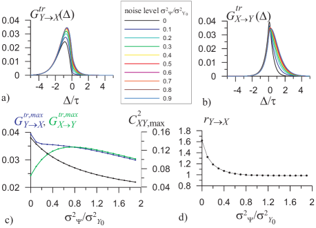
Figure 2: Causality measures depending on observational noise level $\sigma_{\Psi}^{2}$ for the system (17) at $h/\tau=0.2$, $\sigma_{\Xi}^{2}=0$, $\delta^{Y}=0$, $C^{2}_{X_{0}Y_{0},0}=0.1$, and $l_{X}=l_{XY}=l_{Y}=l_{YX}=1$: (a,b) truncated WG causalities versus time lag for different noise levels; (c) maximal truncated WG causalities (blue and green) and maximal CCF value (black) and (d) causality ratio versus $\sigma_{\Psi}^{2}/\sigma_{Y_{0}}^{2}$.

To distinguish between impacts of observational noise and dating error from data, we can use either (i) assumptions about possible levels of both factors or (ii) shapes of the plots $G^{tr}(\Delta)$. For example, (i) if the noise is hardly greater than $20\%$ in terms of variance, then $r_{Y\to X}<1.1$ may be induced only by a dating error greater than $\tau/2$ (Figs. 2,c,d); (ii) if shapes of the plots $G^{tr}_{Y\to X}(\Delta)$ and $G^{tr}_{X\to Y}(\Delta)$ strongly differ from each other (cf. Figs. 1,a,b and 2,a,b), this is a sign of dating errors rather than observational noise. Being based on exact values of the causality ratio, such considerations are valid only for long enough time series, where statistical fluctuations can be neglected.

6 Note of causality ratio estimation

Much smaller causality ratio estimates (e.g., $0.5$) could appear in practice either due to a violation of Eq. (17) or too short time series. To give an analytic guess for possible statistical fluctuations of time series-based estimates, we note that the estimator $(N/l_{XY})\hat{G}^{tr}_{Y\to X}(\Delta)$ for sufficiently large $N$ roughly follows $\chi^{2}$ distribution with $l_{XY}$ degrees of freedom, so the amplitude of its deviations from the mean for $l_{XY}=1$ equals $3/N$ (the latter is the distance from $0.95$-quantile to the mean) [6]. After maximization over a reasonable interval of the width $2\Delta_{m}=4\tau$, the difference $\delta\hat{G}=\hat{G}^{tr,max}_{Y\to X}(\Delta)-\hat{G}^{tr,max}_{X\to Y}(\Delta)$ for $l_{XY}=l_{YX}=1$ fluctuates with an amplitude of $(3/N)\sqrt{4\cdot 2}\approx 9/N$. Denote the expectation of this difference $\delta G$. Then, $\delta\hat{G}$ and hence the estimator $\hat{r}_{Y\to X}=\hat{G}^{tr,max}_{Y\to X}/\hat{G}^{tr,max}_{X\to Y}$ are slightly affected by statistical fluctuations if the time series length is $N\gg 9/\delta G$. Hence, for a typical $\delta\hat{G}\approx 0.01$ (as in the following example) one should require $N\gg 900$. If a time series is shorter, the role of statistical fluctuations may well appear strong. For a detailed numerical study of such small sample effects, let us focus on situations close to the properties of the palaeoclimate data analyzed below.

7 Causality estimates from palaeoclimate data

A key problem in Climate Sciences is to understand and evaluate relative contributions of different factors to observed global and regional climate variations over time scales on the order of decades and longer. The best sources of such information from the pre-instrumental era are palaeoclimate proxies from different natural archives. One well-dated high-resolution reconstruction has been extracted from the stalagmite YOK-I from Yok Balum Cave (Southern Belize) [25]. The $\delta^{18}O$ record represents local to regional hydroclimate variations in that Atlantic region over the last two millennia with a mean temporal resolution of half a year and is characterized by very low dating errors (up to 17 yrs for ages about 2000 yrs). This time series ($x$ signal) is examined here in parallel with the reconstruction of the total solar irradiance (TSI) based on ¹⁰Be measurements on ice cores [26] to extract information on a possible influence of solar activity ($y$ signal) on the Belize climate over the last two millennia.

The time series are presented in Figs. 3,a,b. The TSI data (Fig. 3,b) have originally been processed to remove the 11-yr solar cycle [26] and sampled in steps of $h=5$ yrs. The original, nonequidistantly sampled YOK-I $\delta^{18}O$ values are shown as red dots in Fig. 3,a, the blue line shows the Gaussian kernel-based filtered[34] record (efficient width of 5 yrs) sampled equidistantly in smaller steps of 1 yr. The sample ACFs of both signals (Fig. 3,c) and their CCF (Fig. 3,d, $\hat{C}^{2}_{XY,max}=0.09$) agree reasonably well with the hypothesis of the relaxators (17) with $\tau\approx 25$ yrs; some deviations may be attributed to statistical fluctuations. The resulting time series length is $N=400$: the signal duration is $80\tau$, the sampling interval is $0.2\tau$.

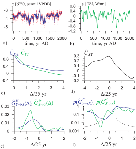
Figure 3: Estimation from palaeoclimate data over the period [15 yr BC - 2010 yr AD]: (a) time series of $\delta^{18}O$ from a speleothem representing local climate (moisture) in the Atlantic region, red points denote the original data, blue line – smoothed signal; (b) time series of solar activity (total solar irradiance); (c) sample ACF for the signals $x$ (blue) and $y$ (green); (d) sample CCF; (e) truncated WG causalities in the directions TSI $\to$ Belize climate (blue) and Belize climate $\to$ TSI (green) for $l_{X}=3$, $l_{XY}=1$, $l_{Y}=4$, $l_{YX}=1$; (f) the respective pointwise $p$-levels for the positivity of $\hat{G}^{tr}_{Y\to X}$ (blue) and $\hat{G}^{tr}_{X\to Y}$ (green), black dashed lines show the pointwise $p$-levels corresponding to the total $p$-level of 0.05 and obtained via the Bonferroni correction [12] with a pre-defined order of tests.

To focus on the most statistically reliable results, we use the model orders selected via the Schwarz criterion for these data ($l_{X}=3$ and $l_{Y}=4$), even though everything is similar for the unit orders. The WG causality estimates differ from zero at least at the level of 0.05: $\hat{G}^{tr,max}_{Y\to X}=0.014$ and $\hat{G}^{tr,max}_{X\to Y}=0.025$ (Figs. 3,e,f). Since $\hat{G}^{tr}_{Y\to X}(\Delta)$ for the direction TSI $\to$ Belize climate is maximal at negative time lag $\Delta$ instead of an expected non-negative lag, a possible dating error can be assumed. It is surprising that the causality ratio from TSI to Belize climate is $\hat{r}_{Y\to X}=0.56$, though we would expect much greater $r_{Y\to X}>1.5$ without observational noise and dating errors and $r_{Y\to X}>0.9$ with those distortions (Figs. 1, 2). Below, we study causality estimators for the same time series length and other parameters and check if statistical fluctuations suffice to explain such a low $\hat{r}_{Y\to X}$.

8 Causality estimates from short time series

Taking $N=400$ and $h/\tau=0.2$, we generated an ensemble of 1000 time series by integrating Eqs. (17) with the Euler – Maruyama technique at time step of $\tau/300$ and imposing (or not) observational noise and dating errors. From each time series, we estimated WG causalities and causality ratio (for $l_{X}=3$, $l_{Y}=4$, $l_{XY}=l_{YX}=1$). Then we calculated their mean values and probabilities to exceed threshold values equal to the respective palaeoclimate estimates [27]. The result is that for this data amount the effect of statistical fluctuations on the causality estimates is considerably stronger than that of dating errors (the second place) and observational noise (the third place).

Without observational noise and dating errors, we specify $k/\alpha=0.45$ which gives CCF close to the palaeoclimate estimate. For smaller $k/\alpha$ (e.g. $\leq 0.3$) the WG causality estimates are insignificant according to the $F$-test, while for greater $k/\alpha$ (e.g. $\geq 0.6$) the CCF and WG causalities estimates considerably exceed the respective palaeoclimate values. The estimation shows that typically $\hat{r}_{y\to x}>1$. A less typical case of $r_{y\to x}<1$ (even down to 0.7) is observed in fewer than $10\%$ of time series in an ensemble. Both WG causality estimates are significant at least at $p=0.05$ in more than $90\%$ of the time series. Appearance of the plots $\hat{G}^{tr}_{Y\to X}(\Delta)$ and $\hat{G}^{tr}_{X\to Y}(\Delta)$ is similar to Figs. 3,e,f, except for the locations of the maxima [27]: statistically significant $\hat{G}^{tr}_{Y\to X}(\Delta)$ has a maximum near zero, not at a negative lag. However, the half-time dating error $\delta^{Y}=0.8\tau=20$ yrs moves the maximum of $\hat{G}^{tr}_{Y\to X}(\Delta)$ to negative lags of $\Delta\approx-\delta^{Y}$ which is observed in about $50\%$ of the ensemble. Thus, the system (17) with dating errors is closer to our palaeoclimate example.

The values of $\hat{r}_{Y\to X}$ depend on various factors [27]. For zero observational noise and zero dating errors the mean of $\hat{r}_{Y\to X}$ is 1.2 which is already low enough as compared to the theoretical $r_{Y\to X}=1.6$, i.e., statistical fluctuations of the estimate already play the role of noise. The ratio $r_{Y\to X}$ decreases very slightly under increasing noise in the driving signal $\sigma_{\Psi}^{2}$ even up to a very large $100\%$ level (at zero noise in the driven signal). The probability to observe values of $\hat{r}_{Y\to X}\leq 0.56$ rises with $\sigma_{\Psi}^{2}$ from 0.03 only up to to 0.05. The estimates of $r_{Y\to X}$ appear more sensitive to the dating error and their mean falls down to 1.1 already for moderate $\delta^{Y}=-0.8\tau$ and the probability of observing $\hat{r}_{Y\to X}\leq 0.56$ rises from 0.03 to 0.06 at $\delta^{Y}=-0.8\tau$ and even to 0.08 at $\delta^{Y}=-2\tau$ suggesting that the dating error is more probable to be of importance here than the observational noise. Overall, for a time series of the considered moderate length, statistical fluctuations are more influential than observational noise and dating errors: the former decrease the causality ratio from 1.6 to 1.2, as compared to the change of the order of 0.1 induced by the dating error and 0.05 by observational noise. Thus, the time series length seems to be the main factor limiting the accuracy of the estimation for the palaeoclimate data at hand. Yet, as justified above, the relative importance of each factor depends on the time series length. In practice, it can be checked ad hoc for a time series at hand as is done here.

To develop a standard test for statistical significance, we note that under the null hypothesis of uncoupled processes the estimator $\hat{r}_{Y\to X}$ resembles the ratio of two $\chi^{2}$-distributed quantities with $l_{XY}$ and $l_{YX}$ degrees of freedom. Maximization of $G^{tr}(\Delta)$ over an interval of width $2\Delta_{m}=4\tau$ consisting of four independent segments corresponds to maximization of $\chi^{2}$-distributed quantity over four independent trials. Numerical simulations show that for $l_{XY}=1$ such a maximization results in the distribution which can be approximated by the $\chi^{2}$ law with two degrees of freedom. Then, $\hat{r}_{Y\to X}$ is distributed according to Fisher’s $F$-law with $(2,2)$ degrees of freedom. However, quality of the approximation reduces for short time series, where Monte-Carlo based estimation seems more reliable.

Additional tests with simulations of a non-equidistant sampling from (17) and a subsequent Gaussian kernel-based filtering (all identical to the palaeoclimate case) show that it slightly increases the likelihood of the causality estimates obtained from the palaeoclimate data. Still, even in case of best correspondence, the system (17) exhibits characteristics similar to those in the palaeoclimate data only in $10\%$ of all realizations. One reason for this limited agreement between the data and the stationary random process (17) can be temporal changes of some characteristics of the processes underlying the proxy records.

9 Nonstationarity of the palaeoclimate processes

We have accounted for a possible nonstationarity by moving window analysis of the palaeoclimate data. The main results are presented in Fig. 4 for two non-overlapping time windows corresponding to the two subsequent millennia. Figs. 4,a,b (the first millennium A.D.) reveal a usual value of the causality ratio $r_{Y\to X}=1.05>1$. Figs. 4,c,d do not reveal any significant couplings for the second millennium A.D. These results suggest a time-varying solar effect on the Belize climate. Similar analysis with moving windows of different lengths suggests that the transition between the two regimes has most probably occurred over the period 1000 to 1300 A.D. A strong influence in the first millennium A.D. would be in line with a northward position of the Intertropical Convergence Zone (ITCZ, see also [24]) and hence increased rainfall in Belize. A reduced solar influence in the second millennium A.D. could result from a southward displaced ITCZ during the Little Ice Age, and thus reduced tropical rain in Belize.

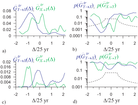
Figure 4: Estimation from two non-overlapping 1000-yr intervals of the palaeoclimate data: (a,b) [15 yr BC – 985 yr AD]; (c,d) [985 yr AD – 1985 yr AD]. Panels (a,c) show truncated WG causalities in the directions TSI $\to$ Belize climate (blue) and Belize climate $\to$ TSI (green) for $l_{X}=3$, $l_{XY}=1$, $l_{Y}=4$, $l_{YX}=1$. Panels (b,d) show pointwise p-levels for positivity of $\hat{G}^{tr}_{Y\to X}$ (blue) and $\hat{G}^{tr}_{X\to Y}$ (green), black dashed lines show pointwise $p$-levels corresponding to the total $p$-level of 0.05.

Our estimates for the first millennium A.D. (Figs. 4,a,b) show that the TSI variations lag the Belize climate proxy by about 20 yrs which seems unacceptable given that TSI should always lead the climatic signal (climatic response to the Sun). Such a lag may well be determined by dating error of at least 20 yrs: Either the age of the solar signal is underestimated or the age of the cave signal is overestimated. Importantly, the question about which signal (or both) has a larger dating error is not possible to answer on the basis of bivariate data. We therefore include the best-dated ice-core based volcanic activity data [13] in our analysis (instead of the TSI data) to check whether its influence on the Belize climate (which is expected and well-accepted) is also characterized by a non-physical negative temporal shift [27]. We have found highly statistically significant volcanic forcing on speleothem $\delta^{18}O$ variations, the maximum of $G^{tr}_{Y\to X}(\Delta)$ being shifted to positive $\Delta=2$ or 3 yrs, i.e. $\Delta\approx h/2$, that agrees with the notion of volcanic forcing delayed by no more than 1 yr. Such a small time delay is totally acceptable. Hence, the test with the volcanic record shows that there is excellent correspondence between eruptions recorded in ice cores and YOK-I which strongly supports the claim of highly accurate dating of the speleothem. Therefore, we conclude that it is the TSI record which is less accurately dated in the first millennium A.D., with a possible age underestimation of about 20 yrs.

10 Conclusions

Dating errors are an almost inevitable characteristic of palaeoclimate time series which makes causality estimation even more difficult. We have proposed the causality ratio $r_{Y\to X}$ based on WG causality (1) as a relevant tool to cope with this problem. We have shown that the value of $r_{Y\to X}>1$ correctly indicates the direction of unidirectional coupling $Y\to X$ for identical stochastic relaxators in the absence of observational noise and dating errors, if the sampling is not too sparse. Only very large observational noise in the driving signal (more than $50\%$ in terms of variance) along with the noise-free driven signal makes $r_{Y\to X}$ close to unity and unsuitable for coupling directionality identification. The causality ratio is more sensitive to the dating error: if half a time series is dated with an error about the relaxation time $\tau$ or greater, $r_{Y\to X}$ gets close to unity again. Hence, in case of a priori known coupling direction, the value of $r_{Y\to X}$ allows to assess likely values of dating errors and observational noise level. However, statistical fluctuations of the estimates from sufficiently short time series may exceed the influence of dating errors and observational noise.

Applying the above results to analyze palaeoclimate data, we confirmed a strong influence of solar activity on the Belize climate over the first millennium A.D. and suggested that this influence strongly decreased in the second millennium. An unexpectedly low causality ratio appears to be determined by the shortness of the time series and, probably, the dating error in the solar proxy over the first millennium A.D. of about 20 yrs, the age of the solar data being underestimated. It seems to be an interesting and fruitful conclusion from an analysis of such a short piece of data on the basis of the adapted causality analysis.

The theoretical part of our research is based on the analysis of a simple, but basic test system (17). Further studies of the influence of dating errors and other factors on WG causalities for more general systems are relevant, including non-identical processes, higher dimensionality of state spaces, and various kinds of nonlinearity. More “inertial” couplings can be analyzed with $l_{XY}>1$ and even with $l_{XY}$ different temporal shifts rather than with a single $\Delta$. All these features will possibly reveal more complicated relationships between the causality ratio and coupling directionality which can then be taken into account, extending the range of applicability of the approach to all fields where dating errors are encountered. Yet, the research presented here is valuable as the first step which already reveals that the adapted WG causality analysis is a promising tool to deal with data corrupted by dating errors and extract information about underlying causal couplings.

11 Supplementary Material

12 Definition of Wiener – Granger causality

Let ($X(t),Y(t)$) be a bivariate random process with $x_{n}=X(nh)$, $y_{n}=Y(nh)$, $n\in{\bf Z}$, $h$ is sampling interval. Self-predictor of $x_{n}$ given by $x^{ind}_{n}=E[x_{n}|x_{n-1},x_{n-2},\dots]$, where $E[\cdot|\cdot]$ stands for a conditional expectation, gives the least (over all self-predictors) mean-squared error $\sigma^{2}_{x,ind}=E[(x_{n}-x^{ind}_{n})^{2}]$. The joint predictor $x^{joint}_{n}=E[x_{n}|x_{n-1},y_{n-1},x_{n-2},y_{n-2},\dots]$ gives the error $\sigma^{2}_{x,joint}$. Normalized prediction improvement value $G_{Y\rightarrow X}=(\sigma^{2}_{x,ind}-\sigma^{2}_{x,joint})/\sigma^{2}_{x,ind}$ is a measure of WG causality in the direction $Y\rightarrow X$, originally called “causality strength” [1]. The idea was suggested in Ref. [2] and realized in Ref. [3] in application to stationary Gaussian process $(x_{n},y_{n})$. The latter yields to a bivariate linear autoregressive (AR) equation

$$\begin{array}[]{rcr}x_{n}&=&\displaystyle\sum_{k=1}^{\infty}{a_{x,k}x_{n-k}}+\sum_{k=1}^{\infty}{b_{x,k}y_{n-k}}+\xi_{n},\\ y_{n}&=&\displaystyle\sum_{k=1}^{\infty}{a_{y,k}y_{n-k}}+\sum_{k=1}^{\infty}{b_{y,k}x_{n-k}}+\psi_{n},\end{array}$$ (7)

where $(\xi_{n},\psi_{n})$ is bivariate zero-mean Gaussian white noise with variances $\sigma^{2}_{\xi}$, $\sigma^{2}_{\psi}$ and covariance $E[\xi_{n}\psi_{n}]=\gamma$. Whiteness assures that $\sigma^{2}_{\xi}=\sigma^{2}_{x,joint}$ and $\sigma^{2}_{\psi}=\sigma^{2}_{y,joint}$ [4]. Similarly, a process $x_{n}$ yields to a univariate AR description, i.e. the first line of Eqs. (7) with all $b_{x,k}=0$ and white noise $\xi^{\prime}_{n}$ with variance $\sigma^{2}_{\xi^{\prime}}=\sigma^{2}_{x,ind}$. Now, $G_{Y\rightarrow X}$ can be determined. Everything is similar for $G_{X\rightarrow Y}$.

13 Estimation of WG causality

In order to estimate the theoretical values $G_{y\rightarrow x}$ from a finite time series $\{x_{n},y_{n}\}_{n=1}^{N}$, one truncates the infinite sums in Eq. (7) at finite numbers of terms and fits truncated univariate and bivariate AR models

$$\begin{array}[]{rcr}x_{n}&=&\displaystyle\sum_{k=1}^{l_{X}}{\tilde{a}_{x,k}x_{n-k}}+\sum_{k=1}^{l_{XY}}{\tilde{b}_{x,k}y_{n-k}}+\tilde{\xi}_{n},\\ y_{n}&=&\displaystyle\sum_{k=1}^{l_{Y}}{\tilde{a}_{y,k}y_{n-k}}+\sum_{k=1}^{l_{YX}}{\tilde{b}_{y,k}x_{n-k}}+\tilde{\psi}_{n},\end{array}$$ (10)

to the data via the ordinary least-squares technique, e.g. [4]. Formally speaking, one uses the predictors $x^{ind}_{n,l_{X}}=E[x_{n}|x_{n-1},x_{n-2},\dots,x_{n-l_{X}}]$ and $x^{joint}_{n,l_{X},l_{XY}}=E[x_{n}|x_{n-1},\dots,x_{n-l_{X}},y_{n-1},\dots,y_{n-l_{XY}}]$. Thereby, one gets truncated WG causality measure $G^{tr}_{Y\rightarrow X}$. The latter is often a good approximation of $G_{Y\rightarrow X}$ already at quite small values of the AR orders $l_{X}$ and $l_{XY}$.

The value of $l_{X}$ is often (and, in particular, in study of the climate data here) selected via the Schwarz criterion [5]. Namely, one minimizes the quantity $\displaystyle\frac{N}{2}\ln{\hat{\sigma}^{2}_{\tilde{\xi}}}+\frac{l_{X}+1}{2}\ln{N}$, where $\hat{\sigma}^{2}_{\tilde{\xi}}$ is the achieved mean-squared error of the one-step AR model prediction. At any value of $l_{XY}$, the pointwise statistical significance level $p(l_{XY})$ (probability of random error) of the conclusion “$G_{Y\to X}>0$” is checked via Fisher’s $F$-test [6]. The value of $l_{XY}$ can also be selected via the Schwarz criterion. Alternatively, it can be selected via minimization of the overall significance level with the account of Bonferroni correction for multiple testing, i.e. via minimization of the value $l_{XY}p(l_{XY})$. In our palaeoclimate example we confine ourselves with $l_{XY}=l_{YX}=1$ based on the Schwarz criterion. Thereby, we finally get an estimate $\hat{G}_{Y\rightarrow X}$.

14 Exact calculation of truncated WG causality

Denote ${\bf R}({\bf z})=\langle{\bf z}\cdot{\bf z}^{\rm T}\rangle$ covariance matrix of a random vector ${\bf z}$, angle brackets stand for expectation. Denote ${\bf x}_{n-1}^{l_{X}}=(x_{n-1},x_{n-2},\dots,x_{n-l_{X}})^{\rm T}$ and ${\bf y}_{n-1}^{l_{XY}}=(y_{n-1},y_{n-2},\dots,y_{n-l_{XY}})^{\rm T}$, where T stands for transposition. To compute $G_{Y\to X}$, one can use the covariance matrices ${\bf R}(x_{n},{\bf x}_{n-1}^{l_{X}})$, ${\bf R}({\bf x}_{n-1}^{l_{X}})$, ${\bf R}(x_{n},{\bf x}_{n-1}^{l_{X}},{\bf y}_{n-1}^{l_{XY}})$, and ${\bf R}({\bf x}_{n-1}^{l_{X}},{\bf y}_{n-1}^{l_{XY}})$ of the respective (conjugated) random vectors. These are square matrices of dimensions $l_{X}+1$, $l_{X}$, $l_{X}+l_{XY}+1$, and $l_{X}+l_{XY}$, respectively. According to Refs. [7, 8, 9], the truncated WG causality for stationary Gaussian processes $x_{n}$ and $y_{n}$ relates to the determinants of these matrices as

$$G_{Y\rightarrow X}^{tr}=1-\displaystyle\frac{|{\bf R}(x_{n},{\bf x}_{n-1}^{l_{X}},{\bf y}_{n-1}^{l_{XY}})|}{|{\bf R}({\bf x}_{n-1}^{l_{X}},{\bf y}_{n-1}^{l_{XY}})|}/\frac{|{\bf R}(x_{n},{\bf x}_{n-1}^{l_{X}})|}{|{\bf R}({\bf x}_{n-1}^{l_{X}})|}.$$ (11)

If $l_{X}=l_{XY}=1$, the right-hand side of Eq. (11) involves only the correlations $C_{XX}(h)$, $C_{XY}(0)$ and $C_{XY}(h)$, where correlation functions are defined as $C_{XX}(lh)=\langle x_{n}x_{n-l}\rangle/\langle x_{n}^{2}\rangle$, $C_{XY}(lh)=\langle x_{n}y_{n-l}\rangle/\sqrt{\langle x_{n}^{2}\rangle\langle y_{n}^{2}\rangle}$, where zero mean of the processes is taken into account and $l$ is integer .

The time-lagged WG causality $G^{tr}_{Y\rightarrow X}(\Delta)$ is defined in full analogy with (11) where ${\bf y}_{n-1}^{l_{XY}}$ is replaced by ${\bf y}_{n-l}$ where $l$ is integer and $\Delta=lh$:

$$G_{Y\rightarrow X}^{tr}(\Delta)=1-\displaystyle\frac{|{\bf R}(x_{n},{\bf x}_{n}^{l_{X}},{\bf y}_{n-l}^{l_{XY}})|}{|{\bf R}({\bf x}_{n}^{l_{X}},{\bf y}_{n-l}^{l_{XY}})|}/\frac{|{\bf R}(x_{n},{\bf x}_{n}^{l_{X}})|}{|{\bf R}({\bf x}_{n}^{l_{X}})|}.$$ (12)

If $l_{X}=l_{XY}=1$, the right-hand side of Eq. (12) involves only the correlations $C_{XX}(h)$, $C_{XY}(\Delta)$ and $C_{XY}(\Delta-h)$.

For a model system specified by stochastic differential equations

$$d{\bf z}/dt={\bf A}\cdot{\bf z}+{\bf\xi},$$ (13)

where ${\bf A}$ is a constant matrix and ${\bf\xi}$ is white noise, all these covariance matrices can be found via standard solution of linear differential equations for the second moments [10]:

$$\frac{d\langle{\bf z}(0)\cdot{\bf z}(-t)^{\rm T}\rangle}{dt}={\bf A}\cdot\langle{\bf z}(0)\cdot{\bf z}(-t)^{\rm T}\rangle.$$ (14)

15 Model system and design of numerical study

To repeat the main text: As a model system, we consider identical first-order decay processes

$$\begin{array}[]{rcl}dX_{0}/dt&=&-\alpha X_{0}(t)+kY_{0}(t)+\zeta_{X}(t),\\ dY_{0}/dt&=&-\alpha Y_{0}(t)+\zeta_{Y}(t),\end{array}$$ (17)

where $\alpha$ determines the characteristic relaxation time $\tau=1/\alpha$, $k$ is the coupling coefficient, and $\zeta_{X}$ and $\zeta_{Y}$ are independent zero-mean white noises with autocorrelation functions $\langle\zeta_{X}(t_{1})\zeta_{X}(t_{2})\rangle=\langle\zeta_{Y}(t_{1})\zeta_{Y}(t_{2})\rangle=\delta(t_{1}-t_{2})$ where $\delta$ is Dirac’s delta. For the system (17) it appears possible to confine ourselves with the orders $l_{X}=l_{XY}=l_{Y}=l_{YX}=1$. The quantity $G^{tr}_{Y\to X}(\Delta)$ at $l_{X}=l_{XY}=1$ coincides exactly with squared partial cross-correlation [11]. Since the covariance matrices are found explicitly for the system (17), we compute the time-lagged truncated WG causalities versus $\Delta$ in the wide range $[-5\tau,5\tau]$ at high resolution of $0.001\tau$ to select their maxima. Thereby, the causality ratio is found at high precision.

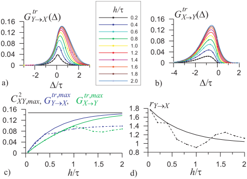
Figure 5: Causality measures for the system (17) at $C^{2}_{X_{0}Y_{0},0}=0.1$ and $l_{X}=l_{XY}=l_{Y}=l_{YX}=1$: (a,b) truncated WG causalities versus time lag for different sampling intervals; (c) maximal truncated WG causalities (blue and green) and maximum CCF value (black) and (d) causality ratio versus sampling interval. Dashed lines in (c) and (d) are for maximization over $\Delta$ varied in steps of $h$, solid lines – for $\Delta$ varied in smaller steps of $0.025\tau$.

16 Causality ratio versus sampling rate and coupling strength

Figs. 5,a,b show $G^{tr}_{Y\to X}(\Delta)$ and $G^{tr}_{X\to Y}(\Delta)$ for various sampling rates at moderate coupling strength corresponding to $C^{2}_{XY,0}=0.1$ ($C^{2}_{XY,max}=0.15$). For a moderate $h=0.2\tau$, the maximum value of $G^{tr}(\Delta)$ in the “correct” direction $Y\to X$ is achieved at small positive $\Delta=h/2$ (the past influences the present), if $\Delta$ is varied at much smaller step than $h$ as is possible when one of the signals is available at such a smaller sampling interval (Fig. 1,a, black line), or at $\Delta=0$, if $\Delta$ is varied in steps of $h$ (black circles). The maximum in the opposite direction $X\to Y$ is achieved at a “nonphysical” negative $\Delta=-\tau$ (Fig. 1,b) as a result of the interdependence between $X(t)$ and $Y(t)$ induced by the $Y\to X$ coupling. This pattern of the maxima locations is characteristic of unidirectional coupling. The causality ratio is $r_{Y\to X}\approx 1.6$ (Fig. 5,d, solid line), which is well above unity. Everything is similar for much smaller $h$, with $r_{Y\to X}\approx 1.8$.

As for the rather sparse sampling with $h\geq\tau$, the ratio $r_{Y\to X}$ gets close to unity, since $G^{tr}_{Y\to X}(\Delta)$ and $G^{tr}_{X\to Y}(\Delta)$ become almost independent of the conditioning variables $x(t-h)$ and $y(t-h)$ tending to the squared CCF (Fig. 5,a-c). For discrete $\Delta$, the ratio $r_{Y\to X}\to 1$ in a non-monotone manner, taking the values as small as 0.9 (Fig. 5,d, dashed line). Thus, only if the sampling interval is of the order of the characteristic time $\tau$, the causality ratio cannot reliably reveal the coupling directionality.

The situation is similar for any coupling strength. Fig. 6,a,b show dependencies of the causality characteristics on $C^{2}_{X_{0}Y_{0},0}$ at $\Delta t/\tau=0.2$. The causality ratio achieves its maximal value of $\approx 3$ at $C^{2}_{X_{0}Y_{0},0}\to 0.5$ when dynamics of the system $X$ is sustained entirely by the system $Y$ and $C_{X_{0}Y_{0},max}=0.86$. The causality ratio remains almost constant and equal to $\approx 1.6$ in the wide range of $C^{2}_{X_{0}Y_{0},0}$ from 0.05 to 0.3 (Fig. 6,b). This range corresponds to the maximal CCF ranging from the (notable) value of 0.27 to the (rather large) value of 0.66. In particular, this range includes the most interesting for us moderate maximal CCFs about 0.3 – 0.4. Thus, if the sampling is not too sparse and cross-correlation is not too low, the causality ratio in the “correct” direction is considerably greater than unity (1.6 and greater) which should allow one to confidently infer coupling direction in practice from a sufficiently long time series.

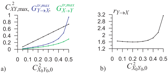
Figure 6: Causality measures for the system (17) at $\Delta t/\tau=0.2$ and $l_{X}=l_{XY}=l_{Y}=l_{YX}=1$ versus squared zero-lag CCF at zero observational noise: (a) Maximal truncated WG causalities (blue and green) and maximal CCF value (black); (d) causality ratio.

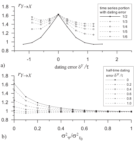
Figure 7: Causality measures for the system (17) at $\Delta t/\tau=0.2$ and $C^{2}_{X_{0}Y_{0},0}=0.1$ (a) versus dating error for zero observational noise and different portions of the time series corrupted by the dating error and (b) versus observational noise level in the driving signal at for $\sigma_{\Xi}^{2}=0$ and different half-time dating errors.

17 Causality ratio versus dating errors and observational noise

Fig. 7,a presents the causality ratio versus dating error for the situation when different portion of the time series $\{y_{n}\}_{n=1}^{N}$ (from 1/2 to 1/6 of the entire series) is corrupted by the dating error. One can see that half-time dating error reduces the value of the causality ratio most strongly (the solid curve). Smaller portions distorted by the uniform dating error lead to a weaker reduction of the causality ratio (dashed curves). Larger uniform error-corrupted portions of 2/3, 3/4, 4/5, and 5/6 lead to the same causality ratio reduction as the smaller complementary ones of 1/3, 1/4, 1/5, and 1/6, respectively (not shown in the plots). Indeed, if the entire series suffers from a uniform dating error, this does not influence the causality ratio since maximization over temporal shifts is involved in the definition of the latter.

Fig. 7,b presents simultaneous influence of the half-time dating error and observational noise in the driving signal $\sigma_{\Psi}^{2}$. One can see that their contributions to the reduction of the causality ratio $r_{y\to x}$ can sum up: e.g. dating error of $0.2\tau$ reduces the causality ratio as compared to zero dating error approximately by 0.15 both for $\sigma_{\Psi}^{2}=0$ and $\sigma_{\Psi}^{2}=0.1\sigma_{Y_{0}}^{2}$, while $\sigma_{\Psi}^{2}=0.1\sigma_{Y_{0}}^{2}$ reduces the causality ratio as compared to $\sigma_{\Psi}^{2}=0$ approximately by 0.3 both for zero dating error and $\delta^{Y}=0.2\tau$. However, for stronger errors of both kinds their effects do not simply add: For dating error of $0.8\tau$ and greater, the causality ratio saturates at the level of unity and the noise does not reduce it any more (and in some range of the noise levels it even increases the causality ratio). Similar saturation of the causality ratio values exists for the noise of about $\sigma_{\Psi}^{2}=0.6\sigma_{Y_{0}}^{2}$ and greater. However, the latter is a huge noise level (about 80 % in root-mean-squared amplitude), while the dating error of $0.8\tau$ is quite realistic for palaeoclimate studies, including the example considered in this work. Thus, the capability of the dating error to decrease $r_{y\to x}$ seems to be stronger and more robust. Still, we note that even the two factors together cannot make $r_{y\to x}$ considerably less than unity, only the ranges of their values leading to $r_{y\to x}\approx 1$ widen in the presence of another factor.

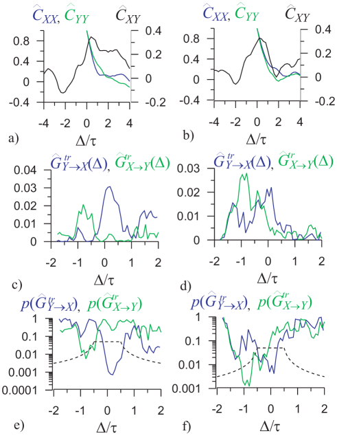
Figure 8: Two examples (left and right column, respectively) of correlation and causality estimates from time series of the system (17) versus time lag at $\Delta t/\tau=0.2$, $\sigma_{\Psi}^{2}=0$, $k=0.0015$, $\delta^{Y}=0$: (a,b) ACF for the signals $x$ (blue) and $y$ (green) and CCF (black); (c,d) WG causality in the directions $Y\to X$ (blue) and $X\to Y$ (green); (e,f) $F$-test based significance level estimates (pointwise p-levels) for positivity of $G_{Y\to X}$ (blue) and $G_{x\to y}$ (green), black dashed lines show the pointwise $p$-level corresponding to the global $p$-level of 0.05 (Bonferroni correction [12] with a pre-defined order of tests).

18 Causality estimates from time series: Numerical simulations

As discussed in the main text, the causality ratio is slightly affected by the estimator fluctuations for the estimated values of palaeoclimate prediction improvements(of the order of 0.01), if the time series length is $N>900$. For the paleoclimate data at hand we have a smaller value of $N=400$ (the signal duration of $80\tau$ at sampling interval $0.2\tau$) so that the role of statistical fluctuations may well appear strong. Therefore, we performed numerical experiments with estimation of WG causalities and causality ratio from time series with the above parameters $N=400$ and $\Delta t/\tau=0.2$ from the system (17) with $\alpha=1/300$ month${}^{-1}=1/25$ yr^-1. To generate the time series, we integrated the with Euler – Maruyama technique with time step of $\tau/300=1$ month and sampling interval of $\Delta t=60$ months which is analogous to the paleoclimate data below. An ensemble of 1000 time series was generated at each set of parameter values. Mean values of WG causalities and causality ratio and probability of them to exceed the respective experimentally observed paleoclimate estimates are computed from each ensemble.

Starting with the case of absent observational noise and dating errors, we specify $k/\alpha=0.45$, i.e. $k=0.0015$ month^-1 which appears overall the most close to the observed paleoclimate data properties. In the selected case, we get mean value of the maximal sample CCF equal to $0.33$ and the probability for it to exceed the paleoclimate value of $0.29$ equal to $0.67$. Here, we present estimates for the truncated WG causality $G^{tr}_{Y\to X}$ for $l_{X}=4,l_{XY}=1$ rather than for $l_{X}=l_{XY}=1$ to be consistent with the paleoclimate example where the orders were selected via the Schwarz criterion. However, numerical experiments show that the causality ratio estimates in these two cases are very close to each other, in particular, their statistics (mean values and probabilities) differ by no more than $1\%$. This is a further confirmation that the above results for $l_{X}=l_{XY}=1$ are correct for (and at least qualitatively agree with) those for higher AR orders, in particular, for the Schwarz criterion-based orders $l_{X},l_{XY}$.

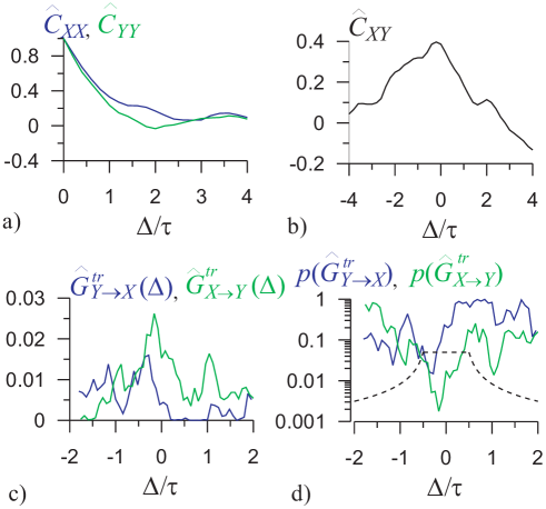
Figure 9: An example of correlation and causality estimates from a time series of the system (17) versus time lag at at $\Delta t/\tau=0.2$, $\sigma_{\Psi}^{2}=0$, $k=0.0015$, half-time dating error $\delta^{Y}/\tau=0.8$: (a) ACF for the signals $x$ (blue) and $y$ (green); (b) CCF; (c) WG causality in the directions $Y\to X$ (blue) and $X\to Y$ (green); (d) pointwise p-levels for positivity of $G_{Y\to X}$ (blue) and $G_{X\to Y}$ (green), black dashed lines show the pointwise $p$-level corresponding to the global $p$-level of 0.05.

Fig. 8 presents two examples of estimates obtained from two different time series of the system (17): left column is the most typical case where the causality ratio $r_{Y\to X}$ is greater than unity (namely about 1.5, Fig. 8,c), right column is less typical case observed in less than for $10\%$ of the time series in the ensemble where $r_{Y\to X}<1$ (namely about 0.7, Fig. 8,d). Both WG causality estimates are statistically significant at least at the level of 0.05 according to the $F$-test with Bonferroni correction, which takes place for more than $90\%$ of the time series in the ensemble. As for ACF and CCF estimates they look quite similar for both cases (Fig. 8,a,b). The right column is quantitatively similar to the paleoclimate example except for the positions of the maxima in WG causality plots. For the correct direction, the maximum is located close to zero in contrast with the paleoclimate example where it is located at a negative lag. Sometimes, the maxima for the correct direction can appear at negative lags in this mathematical example as well, but these cases correspond to statistically insignificant WG causality estimates.

The half-time dating error $\delta^{Y}=-0.8\tau=-20$ yr (Fig. 9) moves the plots for WG causality estimates along the abscissa axis. In particular, the maximum of the plot for the correct direction moves to the negative lags of $\Delta\approx\delta^{Y}$ (Fig. 9,c,d). This location of the maxima is similar to those for paleoclimate data and is observed in about $50\%$ of cases for the analyzed ensemble. Thus, we could say that the system (17) with half-time dating error exhibit some properties close to those for paleoclimate data.

To study a dependence of the estimated causalities on noise level and dating error, let us consider Fig. 10. Note that the mean value of the estimate of the causality ratio $r_{Y\to X}$ is already low enough already for zero noise since statistical fluctuations play the role of noise and move the estimated causality ratio close to unity that the theoretical value (1.2 as compared to 1.6, Fig. 10,a, black line). Fig. 10,a further shows that mean values of WG causalities somewhat decrease with the noise level, but the causality ratio decreases very slightly from 1.2 to 1.17 at the very large $100\%$ noise. As for the probabilities to exceed the fixed “paleoclimate” values, Fig. 10,b shows that they are constant for WG causalities, but for the causality ratio the probability to observe such a low value as 0.56 rises from 0.03 to 0.05 with the noise level. Overall, the causality ratio estimates appear weakly sensitive to observational noise, even though a very large noise makes the observed paleoclimate estimate somewhat more probable, prompting that the solar activity signal might be more noise-corrupted than the Atlantic climate proxy.

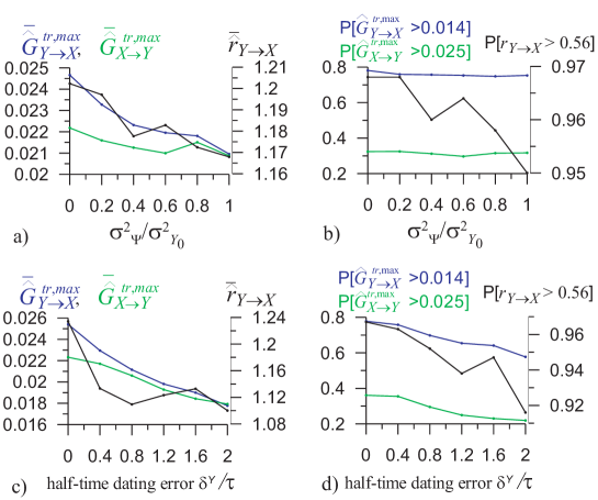
Figure 10: Statistics of the causality estimates for the system (17) depending on observational noise level at zero dating error (a,b) and on half-time dating error at zero observational noise (c,d) over an ensemble of 1000 time series of the length $N=400$ at sampling interval $\Delta t/\tau=0.2$. The left column shows mean values for the maximum truncated WG causalities (blue and green) and the causality ratio (black lines, right ordinate axes). The right column shows probabilities for these estimates to exceed the same estimates obtained from the paleoclimate data.

As for the dating error, Figs. 10,c,d show that the causality ratio estimates are more sensitive to this quantity. Thus, $r_{Y\to X}$ falls down to 1.1 already for moderate $\delta^{Y}=-0.8\tau$ and, more importantly, probability of observing so low causality ratio rises from 0.03 to 0.06 at $\delta^{Y}=-0.8\tau$ and even to 0.08 at $\delta^{Y}=-2\tau$ making the observed paleoclimate estimate of $r_{Y\to X}$ even more probable, prompting that the dating error might well be present in the earlier parts of the paleoclimate data at hand.

Overall, we must state that the contribution of statistical fluctuations is much more important than impacts of the dating error and observational noise. The former circumstance decreases the causality ratio on average from 1.6 to 1.2, as compared to the average change of the order of 0.1 induced by the dating error and 0.05 by the observational noise. Thus, the time series length seems to be the main factor limiting the accuracy of estimation for the paleoclimate data at hand.

19 Estimation of causality between volcanic activity and Yok Balum speleothem-based data

We have performed an additional analysis with quite accurately dated recently published volcanic activity data [13] (Fig. 11). We have revealed that the volcanic activity influences the $\delta^{18}O$ variations with $\Delta=2-3$ yrs (Fig. 11,e,f) which corresponds well with the maximum point $\Delta=h/2$ (which would be equal to 2.5 yrs here) expected for a non-delayed coupling and absent dating errors. The deviation is less than 1 yr. The obtained WG causality estimate is statistically highly significant and the observed small time lag is perfectly acceptable.

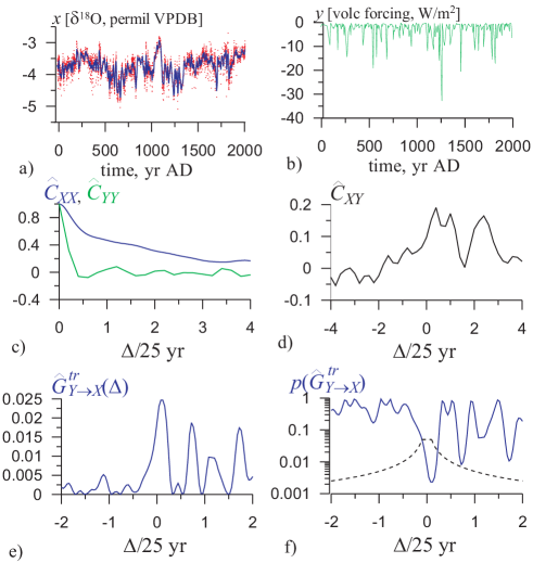
Figure 11: Estimation from palaeoclimate data over the period [15 yr BC - 2010 yr AD]: (a) time series of $\delta^{18}O$ from a speleothem representing local climate (moisture) in the Atlantic region, red points denote the original data, blue line – signal which is smoothed with a Gaussian kernel of the effective width of 5 yrs; (b) an original proxy time series of volcanic activity (global); (c) sample ACF for the signals $x$ (blue) and $y$ smoothed with a Gaussian kernel of 5 yrs width (green); (d) sample CCF; (e) truncated WG causalities in the directions volcanoes $\to$ Belize climate for $l_{X}=3$, $l_{XY}=1$; (f) the respective pointwise $p$-levels for the positivity of $\hat{G}^{tr}_{Y\to X}$, black dashed lines show the pointwise $p$-levels corresponding to the total $p$-level of 0.05.

Considering quite precise dating of the volcanic activity proxy, the above result is a strong argument in favor of an accurate dating of the speleothem data as well. Since we have found a “non-physical” negative lag of total solar irradiance (TSI) variations behind the speleothem-based hydroclimate proxy, we suggest that it is the solar activity signal which might be less accurately dated (with a possible 20 yrs age underestimation, i.e. the TSI record might be in sections too young) rather than the speleothem-based hydroclimate proxy. This notion is corroborated by previous studies, e.g. Ref. [14] (Supplementary material, Figure caption) where the authors also found 22 yrs negative lag (the TSI impossibly following Asian monsoon) and concluded that to be acceptable and within errors.

References

- [1] C.W.J. Granger, Information and Control 6, 18 (1963).
- [2] N. Wiener, in E.F. Beckenbach (ed.) Modern Mathematics for the Engineer (New York: McGraw-Hill, 1956).
- [3] C.W.J. Granger, Econometrica 37 (1969) 424.
- [4] G.E.P. Box and G.M. Jenkins, Time series analysis. Forecasting and control (San Francisco: Holden-Day, 1970).
- [5] G. Schwarz, Ann. Stat. 6, 461 (1978).
- [6] G.A.F. Seber, Linear Regression Analysis (New York: Wiley, 1977).
- [7] L. Barnett, A.B. Barrett, and A.K. Seth, Phys. Rev. Lett. 103 (2009) 238701.
- [8] D.A. Smirnov, Phys. Rev. E 87, 042917 (2013).
- [9] D.W. Hahs and S.D. Pethel, Entropy 15, 767 (2013).
- [10] D.A. Smirnov, Phys. Rev. E 90, 062921 (2014).
- [11] Runge, J. Kurths, and V. Petoukhov, J. Climate 27, 720 (2014).
- [12] E.L. Lehmann, Testing Statistical Hypotheses(New York: Springer, 1986).
- [13] M. Sigl, M. Winstrup, J.R. McConnell1, et al. Nature 523, 543 (2015).
- [14] F. Steinhilber, J.A. Abreu, J. Beer, et al. Proceedings of the National Academy of Sciences 109, 5967 (2012).