Bayesian inference for high-dimensional decomposable graphs

Abstract

In this paper, we consider high-dimensional Gaussian graphical models where the true underlying graph is decomposable. A hierarchical $G$-Wishart prior is proposed to conduct a Bayesian inference for the precision matrix and its graph structure. Although the posterior asymptotics using the $G$-Wishart prior has received increasing attention in recent years, most of results assume moderate high-dimensional settings, where the number of variables $p$ is smaller than the sample size $n$. However, this assumption might not hold in many real applications such as genomics, speech recognition and climatology. Motivated by this gap, we investigate asymptotic properties of posteriors under the high-dimensional setting where $p$ can be much larger than $n$. The pairwise Bayes factor consistency, posterior ratio consistency and graph selection consistency are obtained in this high-dimensional setting. Furthermore, the posterior convergence rate for precision matrices under the matrix $\ell_{1}$-norm is derived, which turns out to coincide with the minimax convergence rate for sparse precision matrices. A simulation study confirms that the proposed Bayesian procedure outperforms competitors.

Key words: $G$-Wishart prior; strong graph selection consistency; posterior convergence rate.

1 Introduction

Consider a sample of observations from a $p$-dimensional normal model

$$X_{1},\ldots,X_{n}\mid\Omega \overset{iid}{\sim} N_{p}(0,\Omega^{-1}),$$

where $\Omega$ is a $p\times p$ precision matrix. The main focus of this paper is estimating the (i) support of the precision matrix and (ii) precision matrix itself. The support recovery of the precision matrix (or equivalently, graph selection) means estimating the locations of nonzero entries of the precision matrix. A statistical inference on a precision matrix, or a covariance matrix $\Sigma=\Omega^{-1}$, is essential to uncover the dependence structure of multivariate data. Especially, a precision matrix reveals the conditional dependences between the variables. However, especially when the number of variables $p$ can be much larger than the sample size $n$, it is a challenging task because a consistent estimation is impossible without further assumptions (Lee and Lee, 2018).

Various restrictive matrix classes have been suggested to enable consistent estimation in such high-dimensional settings. One of the most popular restrictive matrix classes is the set of sparse matrices. The sparsity assumption, which means most of entries of a matrix are zero, can be imposed on covariance matrices (Cai and Zhou, 2012; Cai, Ren and Zhou, 2016), precision matrices (Cai, Liu and Zhou, 2016; Banerjee and Ghosal, 2015) or Cholesky factors (Lee and Lee, 2017; Lee et al., 2019; Cao et al., 2019). In this paper, we focus on sparse precision matrices. They lead to sparse Gaussian graphical models, which will be described in Section 2.2. Various statistical methods have been proposed in the frequentist literature for estimating high-dimensional sparse precision matrices using penalized likelihood estimators (Yuan and Lin, 2007; Rothman et al., 2008; Ravikumar et al., 2011) and neighborhood-based methods (Meinshausen and Bühlmann, 2006; Cai et al., 2011). Ren et al. (2015) and Cai, Liu and Zhou (2016) suggested a regression-based method and an adaptive constrained $\ell_{1}$-minimization method, respectively, and showed that the proposed methods achieve the minimax rates and graph selection consistency for sparse precision matrices.

On the Bayesian side, relatively few works have investigated asymptotic properties of posteriors for high-dimensional precision matrices. The main obstacle is the difficulty of constructing a convenient prior for sparse precision matrices. Because priors have to be defined on the space of sparse positive definite matrices, calculating normalizing constants is a nontrivial issue. Banerjee and Ghosal (2015) used a mixture of point mass at zero and Laplace priors for off-diagonal entries and exponential priors for diagonal entries under the positive definiteness constraint. They obtained the posterior convergence rate for sparse precision matrices under the Frobenius norm, but their result requires the assumption $p=o(n)$. Furthermore, because the marginal posterior of the graph is intractable, they used Laplace approximation. Wang (2015) proposed a similar method by using continuous spike-and-slab priors for off-diagonal entries of precision matrices. However, theoretical properties of the induced posteriors are unavailable, and a Gibbs sampling algorithm should be used due to the unknown normalizing constant.

As an alternative, the $G$-Wishart prior (Atay-Kayis and Massam, 2005) has been widely used to conduct a Bayesian inference for sparse precision matrices. One of advantages of this prior is that the prior density has a closed form if the underlying graph is decomposable, where the definition of a decomposable graph will be given in Section 2.2. Based on the $G$-Wishart prior, Xiang et al. (2015) proved the posterior convergence rate for precision matrices under the matrix $\ell_{\infty}$-norm when the graph is decomposable. However, they assumed that the graph is known, which is rarely true in real applications. Banerjee and Ghosal (2014) also used the $G$-Wishart prior and derived the posterior convergence rate for banded (or bandable) precision matrices, whose entries farther than a certain distance from the diagonal are all zeros (or very small). Since the underlying graph is always decomposable for banded precision matrices, the posterior can be calculated in a closed form. However, in Xiang et al. (2015) and Banerjee and Ghosal (2014), the graph selection consistency of posteriors has not been investigated.

Recently, Niu et al. (2019) and Liu and Martin (2019) investigated asymptotic properties of posteriors using $G$-Wishart priors when the true graph is decomposable and unknown. Niu et al. (2019) established the posterior ratio consistency as well as the graph selection consistency, when $p$ grows to infinity as $n\to\infty$. Liu and Martin (2019) obtained the posterior convergence rate of precision matrices under the Frobenius norm. However, these works assumed a moderate high-dimensional setting, where $p=O(n^{\delta})$ for some $0<\delta<1$. To the best of our knowledge, asymptotic properties of posteriors for decomposable Gaussian graphical models in an ultra high-dimensional setting, say $p\gg n$, have not been established yet.

In this paper, we consider high-dimensional decomposable Gaussian graphical models. A hierarchical $G$-Wishart prior is proposed for sparse precision matrices. We fill the gap in the literature by showing that the proposed Bayesian method achieves the graph selection consistency and the posterior convergence rate in high-dimensional settings, even when $p\gg n$. Under mild conditions, we first show the pairwise Bayes factor consistency (Theorem 3.1) and posterior ratio consistency (Theorem 3.2). Furthermore, the graph selection consistency of posteriors (Theorem 3.3) is shown under slightly stronger conditions. Based on these results, we also show that our method attains the posterior convergence rate for precision matrices (Theorem 3.4) under the matrix $\ell_{1}$-norm, which is faster than the posterior convergence rates obtained in existing literature. Furthermore, the consistency of the posterior mean is established (Theorem 3.5). The practical performance of the proposed method is investigated in simulation studies, which shows that our method outperforms the other frequentist methods.

The rest of paper is organized as follows. In Section 2, we introduce notation, Gaussian graphical models, the hierarchical $G$-Wishart prior and the resulting posterior. In Section 3, we establish asymptotic properties of posteriors such as the graph selection consistency and posterior convergence rate. Simulation studies focusing on both the graph selection and covariance estimation are provided in Section 4, and a discussion is given in Section 5. The proofs of the main results are provided in the Appendix.

2 Preliminaries

2.1 Notation

For any positive sequences $a_{n}$ and $b_{n}$, we denote $a_{n}=o(b_{n})$, or equivalently, $a_{n}\ll b_{n}$, if $a_{n}/b_{n}\longrightarrow 0$ as $n\to\infty$, and $a_{n}=O(b_{n})$, or equivalently, $a_{n}\lesssim b_{n}$, if there exists a constant $C>0$ such that $a_{n}/b_{n}\leq C$ for all sufficiently large $n$. We denote $a_{n}\asymp b_{n}$ if there exist positive constants $C_{1}$ and $C_{2}$ such that $C_{1}\leq a_{n}/b_{n}\leq C_{2}$. For any $p\times p$ matrix $A=(A_{ij})$, $P\subset\{1,\ldots,p\}$ and $1\leq j\leq p$, let $A_{P}=(A_{ij})_{i,j\in P}\in\mathbb{R}^{|P|\times|P|}$ and $A_{Pj}=(A_{ij})_{i\in P}\in\mathbb{R}^{|P|\times 1}$ be submatrices of $A$. For any $p\times p$ matrix $A$, we define the matrix $\ell_{w}$-norm by

$$\|A\|_{w} = \sup_{x\in\mathbb{R}^{p},\|x\|_{w}=1}\|Ax\|_{w}$$

for any integer $1\leq w\leq\infty$, where $\|a\|_{w}$ is the vector $\ell_{w}$-norm for any $a\in\mathbb{R}^{p}$. As special cases, we have

$$\|A\|_{1} = \sup_{x\in\mathbb{R}^{p},\|x\|_{1}=1}\|Ax\|_{1}\,\,=\,\,\max_{1\leq j\leq p}\sum_{i=1}^{p}|A_{ij}|,$$

$$\|A\| = \|A\|_{2}\,\,=\,\,\sup_{x\in\mathbb{R}^{p},\|x\|_{2}=1}\|Ax\|_{2}$$

$$= \big{\{}\lambda_{\max}(A^{T}A)\big{\}}^{1/2},$$

where $\lambda_{\max}(A)$ is the largest eigenvalue of $A$. The matrix $\ell_{2}$-norm, (2.1), is called the spectral norm.

2.2 Gaussian graphical models

Consider an undirected graph by $G=(V,E)$, where $V=\{1,\ldots,p\}=[p]$ and $E\subseteq\{(i,j):i<j,(i,j)\in V\times V\}$. For simplicity, we denote the number of edges in a graph $G$ by $|G|$. Let $P_{G}$ be the set of all $p\times p$ positive definite matrices $\Omega=(\Omega_{ij})$ with $\Omega_{ij}\neq 0$ if and only if $(i,j)\in E$. Suppose that we observe the data from the $p$-dimensional Gaussian graphical model,

$$X_{1},\ldots,X_{n}\mid\Omega \overset{iid}{\sim} N_{p}(0,\Omega^{-1}),$$ (2)

where $\Omega\in P_{G}$ is a precision matrix. Since the graph $G$ is usually unknown, both recovery of the graph $G$ and estimation of the precision matrix $\Omega$ are the main goals of this paper. We consider the high-dimensional setting where $p=p_{n}$ grows to infinity as the sample size $n$ gets larger.

We present here some necessary background on graph theory to be self-contained. A graph is said to be complete if all vertices are joined by an edge, and a complete subgraph that is maximal is called a clique. For given vertices $v$ and $w$ in $V$, a path of length $k$ from $v$ to $w$ is a sequence of distinct vertices $v_{0},v_{1},\ldots,v_{k}$ such that $v_{0}=v$, $v_{k}=w$ and $(v_{i-1},v_{i})\in E$ for all $i=1,\ldots,k$. As a special case, if $v=w$, then the path is called the cycle of length $k$. A chord is an edge between two vertices in a cycle but itself is not a part of the cycle. An undirected graph $G$ is said to be decomposable if every cycle of length greater than or equal to 4 possesses a chord (Lauritzen, 1996). One of the advantages of working with a decomposable graph $G$ is that, for any decomposable graph $G$, there exist a perfect sequence of cliques $P_{1},\ldots,P_{h}$ and the separators $S_{2},\ldots,S_{h}$ defined as $S_{l}=(\cup_{j=1}^{l-1}P_{j})\cap P_{l}$ for $l=2,\ldots,h$ (Lauritzen (1996), Proposition 2.17). Here, a sequence is said to be perfect if every $S_{l}$ is complete and, for all $j>1$, there exists a $l<j$ such that $S_{j}\subseteq P_{l}$. In this paper, we will focus on decomposable graphs mainly to exploit this property.

2.3 Hierarchical $G$-Wishart prior

We consider a hierarchical prior for the precision matrix $\Omega$ in (2). First, we impose the following prior on the graph $G$,

$$\pi(G) \propto \binom{p(p-1)/2}{|G|}^{-1}\exp\big{\{}-|G|\,C_{\tau}\log p\big{\}}\,I(G\in\mathcal{D},\,\,|G|\leq R),$$ (3)

for some constant $C_{\tau}>0$ and positive integer $R$, where $\mathcal{D}$ is a set of all decomposable graphs. The condition $|G|\leq R$ implies that we focus only on the graphs not having too large number of edges. The prior (3) consists of two parts: priors for the graph size and the locations of edges. By using the prior (3), the prior mass decreases exponentially with respect to the graph size $|G|$, and given a graph size, the locations of edges are sampled from a uniform distribution. Similar priors have been commonly used in high-dimensional regression (Castillo et al., 2015; Yang et al., 2016; Martin et al., 2017) and covariance literature (Lee et al., 2019; Liu and Martin, 2019).

For a given graph $G$, we will work with the $G$-Wishart prior (Atay-Kayis and Massam, 2005)

$$\Omega\mid G \sim W_{G}(\nu,A),$$

whose density function is given by

$$\pi(\Omega\mid G) = \frac{1}{I_{G}(\nu,A)}\det(\Omega)^{(\nu-2)/2}\exp\Big{\{}-\frac{1}{2}tr(\Omega A)\Big{\}},\quad\Omega\in P_{G},$$

where $\nu>2$, $A$ is a $p\times p$ positive definite matrix and $I_{G}(\nu,A)$ is the normalizing constant. The normalizing constant can be calculated in a closed form if the graph $G$ is decomposable. The $G$-Wishart prior is one of the most popular prior distributions for precision matrices in Gaussian graphical models. For examples, Banerjee and Ghosal (2014); Xiang et al. (2015) and Liu and Martin (2019) used the $G$-Wishart prior in high-dimensional settings.

There are four hyperparameters in the proposed hierarchical $G$-Wishart prior: $C_{\tau}$, $R$, $\nu$ and $A$. To obtain desired asymptotic properties of posterior, appropriate conditions for hyperparameters will be introduced in Section 3.

2.4 Posterior

For Bayesian inference on the graph $G$ and precision matrix $\Omega$, the joint posterior $\pi(\Omega,G\mid{\bf X}_{n})$ should be calculated. Due to the conjugacy of the $G$-Wishart prior, we have

$$\Omega\mid G,{\bf X}_{n} \overset{ind}{\sim} W_{G}(n+\nu,\,{\bf X}_{n}^{T}{\bf X}_{n}+A),$$

$$\pi(G\mid{\bf X}_{n}) \propto f({\bf X}_{n}\mid G)\pi(G)$$

$$\propto \frac{I_{G}(n+\nu,{\bf X}_{n}^{T}{\bf X}_{n}+A)}{I_{G}(\nu,A)}\pi(G),$$

where ${\bf X}_{n}=(X_{1},\ldots,X_{n})^{T}$ and $f({\bf X}_{n}\mid G)$ is the marginal likelihood

$$f({\bf X}_{n}\mid G) = \int f({\bf X}_{n}\mid\Omega)\pi(\Omega\mid G)d\Omega$$

$$= (2\pi)^{-np/2}\frac{I_{G}(n+\nu,{\bf X}_{n}^{T}{\bf X}_{n}+A)}{I_{G}(\nu,A)}.$$

The posterior samples of $(G,\Omega)$ can be obtained from $\pi(G\mid{\bf X}_{n})$ and $\pi(\Omega\mid G,{\bf X}_{n})$ in turn. Because the marginal posterior $\pi(G\mid{\bf X}_{n})$ is only available up to some unknown normalizing constant, Markov chain Monte Carlo (MCMC) methods such as the Metropolis-Hastings (MH) algorithm should be adopted.

3 Main results

In this section, we show asymptotic properties of the proposed Bayesian procedure in high-dimensional settings. Let $G_{0}=(V,E_{0})$ be the true graph, and $P_{0,1},\ldots,P_{0,h_{0}}$ and $S_{0,2},\ldots,S_{0,h_{0}}$ be the corresponding cliques and separators in a perfect ordering. Let $\Omega_{0}=(\Omega_{0,ij})$ and $\Sigma_{0}=(\Sigma_{0,ij})=\Omega_{0}^{-1}$ be the true precision and covariance matrices, respectively. We assume that the data were generated from the $p$-dimensional Gaussian graphical model with the true precision matrix $\Omega_{0}\in P_{G_{0}}$, i.e.,

$$X_{1},\ldots,X_{n} \overset{iid}{\sim} N_{p}(0,\Omega_{0}^{-1}).$$

For given a random vector $Y=(Y_{1},\ldots,Y_{p})^{T}\sim N_{p}(0,\Sigma_{0})$ and an index set $S\subseteq[p]\setminus\{i,j\}$, we denote $\rho_{ij\mid S}$ as the partial correlation between $Y_{i}$ and $Y_{j}$ given $Y_{S}=(Y_{k})_{k\in S}$, i.e., $\rho_{ij\mid S}=\Sigma_{0,ij\mid S}/(\Sigma_{0,ii\mid S}\Sigma_{0,jj\mid S})^{1/2}$, where $\Sigma_{0,ij\mid S}=\Sigma_{0,ij}-\Sigma_{0,iS}\Sigma_{0,S}^{-1}\Sigma_{0,Sj}$ for any $i,j\in[p]$. If $S=\phi$, then $\rho_{ij\mid S}$ reduces to the correlation between $Y_{i}$ and $Y_{j}$, $\rho_{ij}=\Sigma_{0,ij}/(\Sigma_{0,ii}\Sigma_{0,jj})^{1/2}$.

To obtain desired asymptotic properties of posteriors, we assume the following conditions for the true graph and partial correlations.

(A1) $|G_{0}|\leq R$
(A2) $\max\{|\rho_{ij\mid S\setminus\{i,j\}}|:(i,j)\in E_{0},S\subseteq[p],|S|\leq 3R\}\leq 1-1/\sqrt{(n\vee p)}$
(A3) $\min\{\rho_{ij\mid S\setminus\{i,j\}}^{2}:(i,j)\in E_{0},S\subseteq[p],|S|\leq 3R\}\geq C_{\beta}R^{2}\log(n\vee p)/n$ for some constant $C_{\beta}>0$

Condition (A1) says that the size of the true graph $G_{0}$ is not too large so that it resides in the prior support. In fact, the upper bound for $|G_{0}|$ does not need to be exactly equal to $R$, but just less than $R$. In the literature, Liu and Martin (2019) and Niu et al. (2019) also introduced similar conditions to control the number of true edges in $G_{0}$. Condition (A2) implies that the $i$th and $j$th variables have an imperfect linear relationship. It means that there is no set of variables $S$ with $|S|\leq 3R$ that makes $i$ and $j$ with $(i,j)\in E_{0}$ have a perfectly linear relationship when the effects of those variables are removed. Although $1-1/\sqrt{(n\vee p)}$ is used as an upper bound for simplicity, a more general upper bound, $1-1/(n\vee p)^{c}$ for some constant $c>0$, can be used with a proper change in the lower bound of $C_{\beta}$ in Theorems 3.1 and 3.2. Let $\min_{S\subseteq[p],|S|\leq p}\rho_{ij\mid S\setminus\{i,j\}}$ be the minimum partial correlation, then it is nonzero whenever $(i,j)\in E_{0}$ in a decomposable graph $G_{0}$ (Nie et al., 2017). Condition (A3) gives a lower bound for the nonzero partial correlations $\rho_{ij\mid S\setminus\{i,j\}}$ with $|S|\leq 3R$ rather than $|S|\leq p$. Note that the left-hand side of condition (A3) is nonzero whenever the minimum partial correlation is nonzero. Thus, this is weaker than a condition on the minimum partial correlation. In our theory, this condition corresponds to the beta-min condition in the high-dimensional regression literature, which is essential to obtain selection consistency results (Yang et al., 2016; Martin et al., 2017; Cao et al., 2019). Note that the above conditions are not easy to verify in practice except for some simple situations. For example, they are easily satisfied when the number of variables $p$ is fixed.

(P1) Assume that $\nu$ and $C_{\tau}$ are fixed constants such that $\nu>2$ and $C_{\tau}>0$, respectively. Further assume that $R=C_{r}\{n/\log(n\vee p)\}^{\xi/2}$ and $A=g{\bf X}_{n}^{T}{\bf X}_{n}$, where $g\asymp(n\vee p)^{-\alpha}$ for some constants $C_{r}>0$, $0\leq\xi\leq 1$ and $\alpha>0$.

Here, “P” stands for “prior”. Condition (P1) is a sufficient condition for hyperparameters to guarantee the desired asymptotic properties of posteriors. Together with condition (A1), $R=C_{r}\{n/\log(n\vee p)\}^{\xi/2}$ implies that the number of edges in the true graph $G_{0}$ is at most of order $\{n/\log(n\vee p)\}^{\xi/2}$. By choosing the scale matrix $A=g{\bf X}_{n}^{T}{\bf X}_{n}$, our prior can be seen as an inverse of the hyper-inverse Wishart $g$-prior (Carvalho and Scott, 2009). Niu et al. (2019) used a similar prior with $g=n^{-1}$ as suggested by Carvalho and Scott (2009). Note that the hyperparameter $g$ serves as a penalty term for adding false edges in graphs, thus we essentially use a stronger penalty than Carvalho and Scott (2009) and Niu et al. (2019) if $\alpha>1$.

3.1 Graph selection properties of posteriors

The first property is consistency of pairwise Bayes factors using $G$-Wishart priors. Consider the hypothesis testing problem $H_{0}:G=G_{0}$ versus $H_{1}:G=G_{1}$, for some graph $G_{1}\neq G_{0}$. If we use priors $\Omega\sim W_{G_{0}}(\nu,A)$ and $\Omega\sim W_{G_{1}}(\nu,A)$ under $H_{0}$ and $H_{1}$, respectively, we support either $H_{0}$ or $H_{1}$ based on the Bayes factor $B_{10}({\bf X}_{n}):=f({\bf X}_{n}\mid G_{1})/f({\bf X}_{n}\mid G_{0})$. In general, for a given threshold $C_{th}>0$, we support $H_{1}$ if $\log B_{10}({\bf X}_{n})>C_{th}$, and support $H_{0}$ otherwise. Theorem 3.1 shows that we can consistently support the true hypothesis $H_{0}:G=G_{0}$ based on the pairwise Bayes factor $B_{10}({\bf X}_{n})$ for any $G_{1}\neq G_{0}$.

Theorem 3.1 (Pairwise Bayes factor consistency)

Assume that conditions (A1)–(A3) and (P1) hold with $C_{\beta}>10$ and $\alpha>5/2$. Then, we have

$$\frac{f({\bf X}_{n}\mid G)}{f({\bf X}_{n}\mid G_{0})} \overset{p}{\longrightarrow} 0$$

as $n\to\infty$, for any decomposable graph $G\neq G_{0}$ such that $|G|\leq R$.

Niu et al. (2019) showed the convergence rates of pairwise Bayes factor (BF) (in their Theorem 4.1) on some “good” set $\Delta_{a}$ using $g=n^{-1}$, i.e., $\alpha=1$ in our notation, while we use $\alpha>5/2$ in Theorem 3.1. However, their result neither guarantees the pairwise BF consistency nor $\mathbb{P}_{0}(\Delta_{a})\to 1$ as $n\to\infty$. They showed the pairwise BF consistency (in their Corollary 4.1) under the fixed $p$ setting. In this setting, the proposed model in this paper also can obtain the pairwise BF consistency using $\alpha=1$.

The above condition for the hyperparameter $g$, i.e., $g\asymp(n\vee p)^{-\alpha}$ for $\alpha>5/2$, is an upper bound to obtain the consistency result. In fact, one can use an exponentially decreasing penalty to prove Theorems 3.1 and 3.2 under current conditions, for example, $g\asymp(n\vee p)^{-\tilde{R}\alpha}$ for some $\tilde{R}=\tilde{R}_{n}\to\infty$ as $n\to\infty$ as long as $\tilde{R}=o(R)$.

For the rest, we consider the hierarchical $G$-Wishart prior described in Section 2.3. Theorem 3.2 shows what we call as the posterior ratio consistency. Note that the consistency of pairwise Bayes factors does not guarantee the posterior ratio consistency, and vice versa. As a by-product of Theorem 3.2, it can be shown that the posterior mode, $\widehat{G}=\operatorname*{argmax}_{G}\pi(G\mid{\bf X}_{n})$, is a consistent estimator of the true graph $G_{0}$.

Theorem 3.2 (Posterior ratio consistency)

Assume that conditions (A1)–(A3) and (P1) hold with $C_{\beta}>10$ and $\alpha+C_{\tau}>3$. Then, we have

$$\frac{\pi(G\mid{\bf X}_{n})}{\pi(G_{0}\mid{\bf X}_{n})} \overset{p}{\longrightarrow} 0$$

as $n\to\infty$, for any decomposable graph $G\neq G_{0}$.

To obtain the posterior ratio consistency, Niu et al. (2019) assumed $p=O(n^{\alpha_{1}})$ for some $0<\alpha_{1}<1/2$, whereas we do not have any condition on the relationship between $n$ and $p$ as long as $p\to\infty$ as $n\to\infty$. They also assumed $|G_{0}|=O(n^{\sigma})$, $1-\max_{(i,j)\in E_{0}}\rho^{2}_{ij\mid V\setminus\{i,j\}}\asymp n^{-k}$ and $\min_{(i,j)\in E_{0}}\rho^{2}_{ij\mid V\setminus\{i,j\}}\asymp n^{-\lambda}$, for some constants $0\leq\sigma\leq 2\alpha_{1},k\geq 0$ and $0\leq\lambda<\min(\alpha_{1},1/2-\alpha_{1})$, which correspond to conditions (A1), (A2) and (A3) in this paper, respectively. However, the comparison with our result is not straightforward because they imposed conditions on $\max_{(i,j)\in E_{0}}\rho^{2}_{ij\mid V\setminus\{i,j\}}$ and $\min_{(i,j)\in E_{0}}\rho^{2}_{ij\mid V\setminus\{i,j\}}$, whereas we impose conditions on $\max_{(i,j)\in E_{0},|S|\leq R}\rho^{2}_{ij\mid S\setminus\{i,j\}}$ and $\min_{(i,j)\in E_{0},|S|\leq R}\rho^{2}_{ij\mid S\setminus\{i,j\}}$.

Next we show the strong graph selection consistency, which is much stronger than the posterior ratio consistency. To prove Theorem 3.3, we require the following conditions instead of conditions (A3) and (P1):

(B3) $\min\{\rho_{ij\mid S\setminus\{i,j\}}^{2}:(i,j)\in E_{0},S\subseteq[p],|S|\leq 3R\}\geq C_{\beta}R^{3}\log(n\vee p)/n$ for some constant $C_{\beta}>0$
(P2) Assume that $\nu$ and $C_{\tau}$ are fixed constants such that $\nu>2$ and $C_{\tau}>0$, respectively. Further assume that $R=C_{r}\{n/\log(n\vee p)\}^{\xi/3}$ and $g\asymp(n\vee p)^{-R\alpha}$ for some constants $C_{r}>0$, $0\leq\xi\leq 1$ and $\alpha>0$.

Condition (B3) gives a larger lower bound for the nonzero partial correlations than condition (A3). Condition (P2) implies that we further restrict the size of the true graph and use stronger penalty for adding false edges. Note that if we assume that the size of the true graph is bounded above by a constant $C_{r}$, i.e., assuming $\xi=0$ in condition (P2), then condition (B3) is essentially equivalent to (A3) in terms of the rate.

Theorem 3.3 (Strong graph selection consistency)

Assume that conditions (A1), (A2), (B3) and (P2) hold with $C_{\beta}>6$ and $\alpha>3$. Then, we have

$$\pi\big{(}G=G_{0}\mid{\bf X}_{n}\big{)} \overset{p}{\longrightarrow} 1$$

as $n\to\infty$.

Niu et al. (2019) also obtained the strong graph selection consistency under slightly stronger conditions than those they used to prove the posterior ratio consistency. However, their result holds only when $p=o(n^{1/3})$, which does not include the ultra high-dimensional setting, $p\gg n$.

In Theorem 3.3, we use stronger penalty $g\asymp(n\vee p)^{-R\alpha}$ compared with Theorems 3.1 and 3.2. Note that, in Theorems 3.1 and 3.2, we only need to focus on $f({\bf X}_{n}\mid G)$ or $\pi(G\mid{\bf X}_{n})$ for a given graph $G$. However, to prove Theorem 3.3, we should deal with multiple graphs simultaneously; for example, it is required that $\pi\big{(}G\subsetneq G_{0}\mid{\bf X}_{n}\big{)}$ converges to zero in probability as $n\to\infty$, where we need to control multiple graphs, $\{G:G\subsetneq G_{0}\}$, simultaneously. To this end, a strong penalty $g\asymp(n\vee p)^{-R\alpha}$ is required to prove Theorem 3.3 using current techniques.

3.2 Posterior convergence rate for precision matrices

In this section, we establish the posterior convergence rate for high-dimensional precision matrices under the matrix $\ell_{1}$-norm using the proposed hierarchical $G$-Wishart prior. To obtain the posterior convergence rate, we further assume the following condition:

(B4) There exists a constant $\epsilon_{0}>0$ such that $\epsilon_{0}\leq\lambda_{\min}(\Omega_{0})\leq\lambda_{\max}(\Omega_{0})\leq\epsilon_{0}^{-1}$, where $\lambda_{\min}(\Omega_{0})$ is the smallest eigenvalue of $\Omega_{0}$.

Condition (B4) is the well-known bounded eigenvalue condition for $\Omega_{0}$, and similar conditions can be found in Ren et al. (2015), Banerjee and Ghosal (2015) and Liu and Martin (2019). Recently, Liu and Martin (2019) obtained the posterior convergence rate for precision matrices under the Frobenius norm without the beta-min condition like condition (B3). However, they assumed a moderate high-dimensional setting, $p+|G_{0}|=o(n/\log p)$. Theorem 3.4 shows the posterior convergence rate of the hierarchical $G$-Wishart prior under the matrix $\ell_{1}$-norm in high-dimensional settings, including $p\gg n$.

Theorem 3.4 (Posterior convergence rate)

Assume that conditions (A1), (A2), (B3), (B4) and (P2) hold with $C_{\beta}>6$ and $\alpha>3$. Then, if $\log p=o(n)$,

$$\mathbb{E}_{0}\Big{\{}\pi\Big{(}\|\Omega-\Omega_{0}\|_{1}\geq M\tilde{s}_{0}^{2}\sqrt{\frac{\log(n\vee p)}{n}}\mid{\bf X}_{n}\Big{)}\Big{\}} \longrightarrow 0$$ (4)

as $n\to\infty$ for some constant $M>0$, where $\tilde{s}_{0}:=\max_{1\leq j\leq p}\sum_{i=1}^{p}I(\Omega_{0,ij}\neq 0)$, and $\mathbb{E}_{0}$ denotes the expectation corresponding to the model (2) with $\Omega=\Omega_{0}$.

Using the $G$-Wishart prior, Xiang et al. (2015) obtained a larger posterior convergence rate, $\tilde{s}_{0}^{5/2}\{\log(n\vee p)/n\}^{1/2}$, for a precision matrix $\Omega_{0}\in\mathcal{P}_{G_{0}}$, where $G_{0}$ is decomposable and known. Banerjee and Ghosal (2014) derived the same posterior convergence rate for banded precision matrices. It was unclear whether the posterior convergence rate $\tilde{s}_{0}^{5/2}\{\log(n\vee p)/n\}^{1/2}$ using the $G$-Wishart prior can be improved or not. Our result reveals that this rate can be improved even when the true graph $G_{0}$ is unknown.

When a point estimation of precision matrices is of interest, one might want to use a consistent Bayes estimator. However, in general, a posterior convergence rate result does not imply the consistency of the Bayes estimator without further conditions. In the following theorem, we show the conditional posterior mean, $\mathbb{E}^{\pi}(\Omega\mid\widehat{G},\mathbf{X}_{n})$, is a consistent estimator, and its convergence rate under the matrix $\ell_{1}$-norm coincides with the posterior convergence rate in Theorem 3.4. Note that the closed form of $\mathbb{E}^{\pi}(\Omega\mid\hat{G},\mathbf{X}_{n})$ is available because the posterior mode $\widehat{G}$ is decomposable.

Theorem 3.5 (Consistency of Bayes estimator)

Under the same conditions in Theorem 3.4, we have

$$\mathbb{P}_{0}\bigg{(}\,\big{\|}\mathbb{E}^{\pi}(\Omega\mid\widehat{G},\mathbf{X}_{n})-\Omega_{0}\big{\|}_{1}\geq M\tilde{s}_{0}^{2}\sqrt{\frac{\log(n\vee p)}{n}}\,\,\bigg{)} \longrightarrow 0$$

as $n\to\infty$ for some constant $M>0$.

4 Simulation Studies

4.1 Simulation I: Illustration of posterior ratio consistency

In this section, we illustrate the posterior ratio consistency results in Theorem 3.2 using a simulation experiment. First note that for a complete graph $G$, the explicit expression of the normalizing constant in the $G$-Wishart prior is given by

$$I_{G}(\nu,A)=\frac{2^{(\nu+p-1)p/2}\pi^{p(p-1)/4}\prod_{i=0}^{p-1}\Gamma\left(\frac{\nu+p-1-i}{2}\right)}{\left\{\det(A)\right\}^{\frac{\nu+p-1}{2}}}.$$ (5)

As shown in Roverato (2000) and Banerjee and Ghosal (2014), for any decomposable graph $G$ with the set of cliques $\{C_{1},\ldots,C_{h}\}$ and the set of separators $\{S_{2},\ldots,S_{h}\}$, the following holds:

$$I_{G}(\nu,A)=\frac{\prod_{j=1}^{h}I_{C_{j}}\left(\nu,A_{C_{j}}\right)}{\prod_{j=2}^{h}I_{S_{j}}\left(\nu,A_{S_{j}}\right)},$$ (6)

where $A_{C_{j}}$ denotes the submatrix of $A$ formed by its columns and rows of indexed in $C_{j}$. Note that $I_{C_{j}}(\cdot,\cdot)$ and $I_{S_{j}}(\cdot,\cdot)$ can be computed using (5) because $C_{j}$ and $S_{j}$ are complete for any decomposable graph $G$. Further note that the explicit form of the marginal likelihood is given by

$$f({\bf X}_{n}\mid G) = (2\pi)^{-np/2}\frac{I_{G}\left(n+\nu,{\bf X}_{n}^{T}{\bf X}_{n}+A\right)}{I_{G}(\nu,A)}.$$

It then follows from (6) that for any decomposable graph $G$, we have

$$f({\bf X}_{n}\mid G)=(2\pi)^{-np/2}\frac{\prod_{j=1}^{h}I_{C_{j}}\left(n+\nu,({\bf X}_{n}^{T}{\bf X}_{n}+A)_{C_{j}}\right)}{\prod_{j=2}^{h}I_{S_{j}}\left(n+\nu,({\bf X}_{n}^{T}{\bf X}_{n}+A)_{S_{j}}\right)}\frac{\prod_{j=2}^{h}I_{S_{j}}\left(\nu,A_{S_{j}}\right)}{\prod_{j=1}^{h}I_{C_{j}}\left(\nu,A_{C_{j}}\right)}.$$ (7)

Therefore, we can use (7) and prior (3) to compute the posterior ratio between any two decomposable graphs.

Next, we consider seven different values of $p$ ranging from $50$ to $350$, and fix $n=150$. Then, for each fixed $p$, we construct a $p\times p$ covariance matrix $\Sigma_{0,ij}=0.5^{|i-j|}$ for $1\leq i,j\leq p$ such that the inverse covariance matrix $\Omega_{0}=\Sigma_{0}^{-1}$ will possess a banded structure, i.e., the so-called AR(1) model. The matrix $\Omega_{0}$ also gives us the structure of the true underlying graph $G_{0}$. Next, we generate $n$ random samples from $N_{p}(0,\Sigma_{0})$ to construct our data matrix ${\bf X}_{n}$, and set the hyperparameters as $A=0.1\delta^{-1}p^{-2.5-\delta}{\bf X}_{n}^{T}{\bf X}_{n}$, $\delta=0.01$, $\nu=3$ and $C_{\tau}=0.5$. The above process ensures all the assumptions in our Theorem 3.2 are satisfied. We then examine the posterior ratio under four different cases by computing the log of posterior ratio of a “non-true” decomposable graph $G$ and $G_{0}$, $\log\{\pi(G\mid{\bf X}_{n})/\pi(G_{0}\mid{\bf X}_{n})\}$, as follows.

1. Case 1: $G$ is a supergraph of $G_{0}$ and the number of total edges of $G$ is exactly twice of $G_{0}$, i.e. $|G|=2|G_{0}|$.

2. Case 2: $G$ is a subgraph of $G_{0}$ and the number of total edges of $G$ is exactly half of $G_{0}$, i.e. $|G|=\frac{1}{2}|G_{0}|$.

3. Case 3: $G$ is not necessarily a supergraph of $G_{0}$, but the number of total edges of $G$ is twice of $|G_{0}|$.

4. Case 4: $G$ is not necessarily a subgraph of $G_{0}$, but the number of total edges of $G$ is half of $|G_{0}|$.

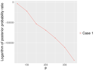
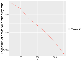
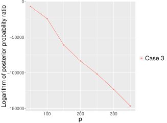
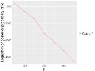
Figure 1: Logarithm of posterior probability ratio for $G$ and $G_{0}$ for various choices of the “non-true” graph $G$.

The logarithms of the posterior ratio for various cases are provided in Figure 1. As expected in all four cases, the logarithm of the posterior ratio decreases as $p$ becomes large. Based on the proof of Theorem 3.2, we can see that the posterior ratio $\pi(G\mid\mathbf{X}_{n})/\pi(G_{0}\mid\mathbf{X}_{n})$ converges in probability to zero as $(n\vee p)\to\infty$. Thus, this result provides a numerical illustration of Theorem 3.2.

4.2 Simulation II: Illustration of graph selection

In this section, we perform the graph selection procedure under the proposed hierarchical $G$-Wishart prior and evaluate its performance along with other competing methods. Recall that the marginal posterior for $G$ is given by

$$\pi(G\mid{\bf X}_{n}) \propto f({\bf X}_{n}\mid G)\pi(G)$$

$$\propto \frac{I_{G}(n+\nu,{\bf X}_{n}^{T}{\bf X}_{n}+A)}{I_{G}(\nu,A)}\pi(G)$$

and available up to some unknown normalizing constant. We thereby suggest using the following MH algorithm for posterior inference:

1. Set the initial value $G^{(1)}$.

2. For each $s=2,\ldots,S$,

   1. sample $G^{new}\sim q(\cdot\mid G^{(s-1)})$ until $G^{new}$ is decomposable;

   2. set $G^{(s)}=G^{new}$ with the probability

      $$p_{acc} = \min\left\{1,\frac{\pi(G^{new}\mid{\bf X}_{n})}{\pi(G^{(s-1)}\mid{\bf X}_{n})}\frac{q(G^{(s-1)}\mid G^{new})}{q(G^{new}\mid G^{(s-1)})}\right\},$$

      otherwise set $G^{(s)}=G^{(s-1)}$.

In the above Step 2(a), we verify whether the resulting graph from local perturbations of the current graph is still decomposable by accepting only those moves that satisfy two conditions outlined in Green and Thomas (2013) on the junction tree representation of the proposed graph. The proposal kernel $q(\cdot\mid G^{\prime})$ is chosen such that a new graph $G^{new}$ is sampled by changing a randomly chosen nonzero entry in the lower triangular part of the adjacency matrix for $G^{\prime}$ to $0$ with probability $0.5$ or by changing a randomly chosen zero entry to $1$ randomly with probability $0.5$. We will refer to our proposed method as the MCMC-based graph selection with hierarchical $G$-Wishart distribution (HGW-M).

Following the simulation settings in Yuan and Lin (2007) and Friedman et al. (2007), we consider five different structures of the true graph, which corresponds to the following sparsity patterns of the true inverse covariance matrix with all the unit diagonals.

1. Setting 1: AR(1) model with ${\Omega}_{i,i-1}={\Omega}_{i-1,i}=0.5$ for $1\leq i\leq p-1$.

2. Setting 2: AR(2) model with ${\Omega}_{i,i-1}={\Omega}_{i-1,i}=0.5$ for $1\leq i\leq p-1$ and ${\Omega}_{i,i-2}={\Omega}_{i-2,i}=0.25$ for $1\leq i\leq p-2$.

3. Setting 3: AR(4) model with ${\Omega}_{i,i-1}={\Omega}_{i-1,i}=0.4$ for $1\leq i\leq p-1$, ${\Omega}_{i,i-2}={\Omega}_{i-2,i}=0.2$ for $1\leq i\leq p-2$, ${\Omega}_{i,i-3}={\Omega}_{i-3,i}=0.2$ for $1\leq i\leq p-3$, and ${\Omega}_{i,i-4}={\Omega}_{i-4,i}=0.1$ for $1\leq i\leq p-4$.

4. Setting 4: Star model where every node connects to the first node, with $\Omega_{1,i}=\Omega_{i,1}=0.2$ for $2\leq i\leq p$, and the remaining entries except the diagonals are set to 0.

5. Setting 5: Circle model with ${\Omega}_{i,i-1}={\Omega}_{i-1,i}=0.5$ for $1\leq i\leq p-1$, $\Omega_{1,p}=\Omega_{p,1}=0.4$, and the remaining entries except the diagonals are set to 0.

For each model, we consider two different values of $p=100$ or 200, and fix $n=100$. Next, under each combination of the true precision matrix and the dimension, we generate $n$ observations from $N_{p}(0,\Sigma_{0})$. The hyperparameters for HGW were set at as $A=(0.1\delta)^{-1}p^{-2.5-\delta}{\bf X}_{n}^{T}{\bf X}_{n}$, $\delta=0.001$, $\nu=3$ and $C_{\tau}=0.5$. The initial state for $G$ was chosen using the graphical lasso (GLasso) (Friedman et al., 2007). For posterior inference, we draw $3,000$ posterior samples with a burn-in period of $3,000$ and collect the indices with posterior inclusion probability larger than $0.5$. Therefore, the final estimate using HGW-M can be regarded as the median probability model graph structure.

To compare the selection performance between the median probability model and the posterior mode, we adopt the hybrid graph selection procedure in Cao et al. (2019) to navigate through the massive posterior space. For all the penalized likelihood methods (Friedman et al., 2007; Cai et al., 2011; Yuan and Lin, 2007), a user-specified penalty parameter controls the level of sparsity of the resulting estimator. Varying values of the penalty parameter provide a range of possible graphs to choose from. This set of graphs is referred to as the solution path. The choice of the penalty parameter is typically made by assigning a BIC-like score to each graph on the solution path, and choosing the graph with the highest score (Cao et al., 2019). For the Bayesian approach, the posterior probabilities naturally assign a score for all the decomposable graph, but the entire graph space is prohibitively large to search in high-dimensional settings. To address this, in the context of Gaussian directed acyclic graphical models, Ben-David et al. (2015) and Cao et al. (2019) develop a computationally feasible approach which searches around the graphs on the penalized likelihood solution path, and demonstrate that significant improvement in accuracy can be obtained by searching beyond the penalized likelihood solution paths using posterior probabilities. Adapted to our setting, we first vary the tuning parameter in GLasso on a grid from 0.01 to 1.5. For each fixed parameter, we further threshold the inverse covariance matrix estimated by GLasso on a grid from 0 to 0.5 to get a sequence of $5,000$ graphs, and include them in the candidate set. We use the same technique in Section 4.2 to ensure the candidate graphs are decomposable. The log posterior probabilities are computed for all candidate graphs, and the one with the highest probability is retained. The shotgun stochastic search is implemented to search around the selected graph and to target the posterior mode $\hat{G}$ (Jones et al., 2005). We refer to this hybrid graph selection approach as HGW-$\hat{G}$.

The performance of HGW-M and HGW-$\hat{G}$ will be compared with other existing methods including the GLasso (Friedman et al., 2007), the constrained $\ell_{1}$-minimization for inverse matrix estimation (CLIME) (Cai et al., 2011) and the tuning-insensitive approach for optimally estimating Gaussian graphical models (TIGER) (Liu and Wang, 2017). The tuning parameters for GLasso and TIGER were chosen by the criterion of StARS, the stability-based method for choosing the regularization parameter in high dimensional inference for undirected graphs (Liu et al., 2010). The penalty parameter for CLIME was selected by 10-fold cross-validation. For GLasso and TIGER, the final model is determined by collecting the nonzero entries in the estimated precision matrix. Since CLIME could not produce exact zeros in our simulation settings, we constructed the final support by thresholding the absolute values of the estimated precision matrix at 0.025.

To evaluate the performance of variable selection, the precision, sensitivity, specificity and Matthews correlation coefficient (MCC) are reported at Tables 1 to 4, where each simulation setting is repeated for 20 times. The criteria are defined as

Precision $$= \frac{\mbox{TP}}{\mbox{TP}+\mbox{FP}},$$

Sensitivitiy $$= \frac{\mbox{TP}}{\mbox{TP}+\mbox{FN}},$$

Specificity $$= \frac{\mbox{TN}}{\mbox{TN}+\mbox{FP}},$$

MCC $$= \frac{\mbox{TP}\times\mbox{TN}-\mbox{FP}\times\mbox{FN}}{\sqrt{(\mbox{TP}+\mbox{FP})(\mbox{TP}+\mbox{FN})(\mbox{TN}+\mbox{FP})(\mbox{TP}+\mbox{FN})}},$$

where TP, TN, FP and FN are true positive, true negative, false positive and false negative, respectively. For a clear visualization, in Figure 2, we plot the heatmaps for comparing the sparsity structure of the precision matrix estimated by different methods under the AR(1) setting and $p=100$.

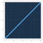
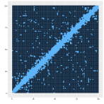
Figure 2: Heatmap comparison of the sparsity structure estimated by different methods under the AR(1) setting. Left to right: HGW-M, HGW-$\hat{G}$, GLasso, CLIME, TIGER.

Setting	$p$	Method	Precision	Sensitivity	Specificity	MCC
AR(1)	100	HGW-M	1	1	1	1
		HGW-$\hat{G}$	1	1	1	1
		GLasso	0.15	1	0.89	0.37
		CLIME	0.17	1	0.90	0.40
		TIGER	0.14	1	0.88	0.36
AR(1)	200	HGW-M	1	1	1	1
		HGW-$\hat{G}$	0.99	1	1	0.99
		GLasso	0.12	0.99	0.93	0.33
		CLIME	0.14	1	0.94	0.37
		TIGER	0.11	1	0.91	0.31

Table 1: The summary statistics for graph selection under the AR(1) setting with various dimensions are reported for each method.

Setting	$p$	Method	Precision	Sensitivity	Specificity	MCC
AR(2)	100	HGW-M	0.94	0.57	1	0.73
		HGW-$\hat{G}$	0.98	0.57	1	0.74
		GLasso	0.24	0.72	0.91	0.38
		CLIME	0.27	0.86	0.91	0.45
		TIGER	0.23	0.73	0.90	0.36
AR(2)	200	HGW-M	0.91	0.49	1	0.66
		HGW-$\hat{G}$	0.96	0.45	1	0.65
		GLasso	0.19	0.72	0.94	0.35
		CLIME	0.12	0.82	0.88	0.29
		TIGER	0.16	0.75	0.92	0.32

Table 2: The summary statistics for graph selection under the AR(2) setting with various dimensions are reported for each method.

Setting	$p$	Method	Precision	Sensitivity	Specificity	MCC
AR(4)	100	HGW-M	0.96	0.13	1	0.33
		HGW-$\hat{G}$	0.98	0.13	1	0.34
		GLasso	0.32	0.29	0.95	0.25
		CLIME	0.25	0.40	0.89	0.24
		TIGER	0.27	0.31	0.93	0.23
AR(4)	200	HGW-M	0.81	0.12	1	0.30
		HGW-$\hat{G}$	0.85	0.12	1	0.31
		GLasso	0.21	0.27	0.96	0.21
		CLIME	0.11	0.35	0.88	0.13
		TIGER	0.19	0.29	0.95	0.19

Table 3: The summary statistics for graph selection under the AR(4) setting with various dimensions are reported for each method.

Setting	$p$	Method	Precision	Sensitivity	Specificity	MCC
Star	100	HGW-M	1	1	1	1
		HGW-$\hat{G}$	0.99	1	1	0.99
		GLasso	0.38	1	0.97	0.61
		CLIME	0.13	0.79	0.90	0.30
		TIGER	0.33	1	0.96	0.56
Circle	200	HGW-M	1	1	1	0.99
		HGW-$\hat{G}$	0.99	0.99	1	0.99
		GLasso	0.31	1	0.98	0.55
		CLIME	0.08	1	0.87	0.26
		TIGER	0.28	1	0.97	0.52

Table 4: The summary statistics for graph selection under Setting 4 and Setting 5 with various dimensions are reported for each method.

Based on the simulation results, we notice that our methods overall work better than the regularization methods across various settings. Our methods perform particularly well in the sparse models under the AR(1), Star and Circle settings. This is because the consistency conditions of HGW are easier to satisfy under sparse settings. Note that when the posterior probability is larger than $1/2$, the median probability model based on HGW-M coincides with the posterior mode based on HGW-$\hat{G}$ (Barbieri and Berger, 2004). Because we have proved the strong selection consistency (Theorem 3.3), the two models should be asymptotically equivalent. This is indeed reflected in our simulations, as we notice HGW-M and HGW-$\hat{G}$ perform comparably well in most settings. Generally speaking, the proposed methods are able to achieve better specificity and precision, while the regularization methods have better sensitivity. The poor specificity of the regularization methods is in accordance with previous work demonstrating that selection of the regularization parameter using cross-validation is optimal with respect to prediction but tends to include more noise predictors compared with Bayesian methods (Meinshausen and Bühlmann, 2006). Overall, our simulation studies indicate that the proposed method can perform well under a variety of configurations with different dimensions, sparsity levels and correlation structures.

4.3 Simulation III: Illustration of inverse covariance estimation

In this section, we provide the performance comparison for the inverse covariance estimation using different methods. For each fixed $p$, the true inverse covariance matrix and the subsequent dataset, are generated by the same mechanism as in Section 4.2. To use HGW-M for the estimation, within each iteration, we sample $\Omega^{(s)}\sim W_{G^{(s)}}(n+\nu,\,{\bf X}_{n}^{T}{\bf X}_{n}+A)$ after Step 2(b), and construct our final estimate by taking the average of all the $\Omega^{(s)}$ after a burn-in period. In terms of the Bayes estimators based on the posterior mode, since the posterior mode is also decomposable, the Bayes estimators can be explicitly derived for that graph under various loss functions (Rajaratnam et al., 2008; Banerjee and Ghosal, 2014). Given the posterior mode, we consider two Bayes estimators $\hat{\Omega}^{\ell_{1}}$ and $\hat{\Omega}^{\ell_{2}}$ corresponding to the $\ell_{1}$ Stein’s loss and $\ell_{2}$ squared-error loss, respectively. The estimated inverse covariance matrices based on other frequentist approaches are obtained as specified in Section 4.2. To evaluate the performance of covariance estimation, different criteria for measuring the estimation loss are reported at Tables 5 to 8, where each simulation setting is repeated for 20 times. Relative errors are chosen as criteria. Specifically, for a matrix norm $\|\cdot\|$ and an estimator $\hat{\Omega}$, the relative error is defined as $\|\Omega_{0}-\hat{\Omega}\|/\|\Omega_{0}\|$. In Tables 5–8, $E_{1}$, $E_{2}$, $E_{3}$ and $E_{4}$ represent the relative errors based on the matrix $\ell_{1}$-norm, the matrix $\ell_{2}$-norm (spectral norm), the vector $\ell_{2}$-norm (Frobenius norm) and the vector $\ell_{\infty}$-norm (entrywise maximum norm), respectively.

Setting	$p$	Method	$E_{1}$	$E_{2}$	$E_{3}$	$E_{4}$
AR(1)	100	HGW-M	0.29	0.26	0.11	0.28
		HGW-$\hat{\Omega}^{\ell_{1}}$	0.27	0.24	0.11	0.29
		HGW-$\hat{\Omega}^{\ell_{2}}$	0.32	0.28	0.11	0.31
		GLasso	0.92	0.88	0.85	0.83
		CLIME	1.02	0.60	0.48	0.37
		TIGER	0.86	0.80	0.76	0.75
AR(1)	200	HGW-M	0.37	0.34	0.15	0.38
		HGW-$\hat{\Omega}^{\ell_{1}}$	0.32	0.27	0.13	0.35
		HGW-$\hat{\Omega}^{\ell_{2}}$	0.35	0.31	0.15	0.40
		GLasso	0.93	0.87	0.84	0.83
		CLIME	1.16	0.64	0.55	0.43
		TIGER	0.88	0.81	0.76	0.75

Table 5: The summary statistics for inverse covariance estimation under the AR(1) setting with various dimensions are reported for each method.

Setting	$p$	Method	$E_{1}$	$E_{2}$	$E_{3}$	$E_{4}$
AR(2)	100	HGW-M	0.68	0.54	0.41	0.49
		HGW-$\hat{\Omega}^{\ell_{1}}$	0.80	0.57	0.39	0.50
		HGW-$\hat{\Omega}^{\ell_{2}}$	0.78	0.56	0.39	0.50
		GLasso	0.85	0.73	0.64	0.55
		CLIME	1.23	0.65	0.58	1.15
		TIGER	0.85	0.72	0.63	0.55
AR(2)	200	HGW-M	0.81	0.64	0.47	0.53
		HGW-$\hat{\Omega}^{\ell_{1}}$	0.80	0.61	0.48	0.52
		HGW-$\hat{\Omega}^{\ell_{2}}$	0.80	0.60	0.47	0.58
		GLasso	0.91	0.74	0.66	0.58
		CLIME	3.48	1.85	1.24	3.95
		TIGER	0.93	0.73	0.64	0.56

Table 6: The summary statistics for inverse covariance estimation under the AR(2) setting with various dimensions are reported for each method.

Setting	$p$	Method	$E_{1}$	$E_{2}$	$E_{3}$	$E_{4}$
AR(4)	100	HGW-M	0.85	0.68	0.53	0.44
		HGW-$\hat{\Omega}^{\ell_{1}}$	0.85	0.65	0.52	0.43
		HGW-$\hat{\Omega}^{\ell_{2}}$	0.84	0.64	0.51	0.42
		GLasso	0.82	0.72	0.6	0.49
		CLIME	1.17	0.48	0.54	0.90
		TIGER	0.84	0.71	0.58	0.48
AR(4)	200	HGW-M	0.94	0.67	0.53	0.59
		HGW-$\hat{\Omega}^{\ell_{1}}$	0.87	0.72	0.57	0.53
		HGW-$\hat{\Omega}^{\ell_{2}}$	0.87	0.71	0.56	0.52
		GLasso	0.88	0.74	0.61	0.50
		CLIME	2.66	1.18	1.01	2.54
		TIGER	0.91	0.73	0.60	0.48

Table 7: The summary statistics for inverse covariance estimation under the AR(4) setting with various dimensions are reported for each method.

Setting	$p$	Method	$E_{1}$	$E_{2}$	$E_{3}$	$E_{4}$
Star	100	HGW-M	0.13	0.19	0.14	0.36
		HGW-$\hat{\Omega}^{\ell_{1}}$	0.13	0.20	0.15	0.36
		HGW-$\hat{\Omega}^{\ell_{2}}$	0.14	0.21	0.15	0.39
		GLasso	0.27	0.29	0.21	0.39
		CLIME	0.83	0.50	0.21	0.42
		TIGER	0.27	0.30	0.21	0.38
Circle	200	HGW-M	0.56	0.44	0.17	0.50
		HGW-$\hat{\Omega}^{\ell_{1}}$	0.56	0.51	0.20	0.52
		HGW-$\hat{\Omega}^{\ell_{2}}$	0.54	0.50	0.18	0.50
		GLasso	0.83	0.76	0.71	0.66
		CLIME	1.14	0.63	0.54	0.40
		TIGER	0.80	0.67	0.61	0.62

Table 8: The summary statistics for inverse covariance estimation under Setting 4 and Setting 5 with various dimensions are reported for each method.

In terms of estimating the inverse covariance matrix, we can tell from the simulation results that our methods overall work better than the regularization methods across various settings. Similar to the performance for uncovering the true sparsity pattern in Section 4.2, our methods can more accurately estimate the magnitudes of the true precision matrix in the sparse models under the AR(1), Star and Circle settings. Different Bayes estimators including the MCMC-based estimator, $\hat{\Omega}^{\ell_{1}}$ and $\hat{\Omega}^{\ell_{2}}$ perform comparably well, which again shows the validity of our theoretical results. Overall, our simulation studies indicate that the proposed method can accommodate a variety of configurations with different dimensions and correlation structures for estimating the inverse covariance matrix.

5 Discussion

In this paper, we assume that the true graph $G_{0}$ is decomposable. Recently, Niu et al. (2019) showed that, even when $G_{0}$ is non-decomposable, the marginal posterior of the graph $G$ concentrates on the space of the minimal triangulation of $G_{0}$. Here, a triangulation of a graph $G=(V,E)$ is a decomposable graph $G^{\Delta}=(V,E\cup F)$, where $F$ is called a set of fill-in edges, and a triangulation is minimal if any only if the removal of any single edge in $F$ leads to a non-decomposable graph. It would be interesting to investigate whether similar properties hold in our setting using the hierarchical $G$-Wishart prior.

Another open problem is whether we can relax the decomposability condition. We assume that the support of the prior is a subset of all decomposable graphs mainly due to technical reasons. By focusing on decomposable graphs, the normalizing constants of posteriors are available in closed forms. This allows us to calculate upper and lower bounds of a posterior ratio. It is unclear to us whether this decomposability condition can be removed. Without this condition, general techniques for obtaining posterior convergence rate, for example, Theorem 8.9 in Ghosal and Van der Vaart (2017), might be needed. Banerjee and Ghosal (2015) used this technique to prove the posterior convergence rate for sparse precision matrices under the Frobenius norm. However, it might be difficult to obtain the posterior convergence rate under the matrix $\ell_{1}$-norm using similar arguments in Banerjee and Ghosal (2015). Let $\epsilon_{n}$ and $\tilde{\epsilon}_{n}$ be the posterior convergence rates for precision matrices under the matrix $\ell_{1}$-norm and Frobenius norm, respectively, where $\epsilon_{n}\ll\tilde{\epsilon}_{n}$. Then, one can see that it is much more difficult to prove the prior thickness (condition (i) of Theorem 8.9 in Ghosal and Van der Vaart (2017)) using $\epsilon_{n}$. Therefore, we suspect that the arguments in Banerjee and Ghosal (2015) cannot be directly applied to our setting.

Appendix A Proofs of main theorems

• If $G\neq G_{0}$, then $G_{0}\subsetneq G$ or $G_{0}\nsubseteq G$. We first focus on the case $G_{0}\subsetneq G$. By Lemma 2.22 in Lauritzen (1996), there exist a sequence of decomposable graphs $G_{0}\subset G_{1}\subset\cdots\subset G_{k-1}\subset G_{k}=G$ with $k=|G|-|G_{0}|$, where $G_{0},G_{1},\ldots,G_{k-1},G_{k}$ differ from by exactly one edge. Then,

  $$\frac{f({\bf X}_{n}\mid G)}{f({\bf X}_{n}\mid G_{0})} = \frac{f({\bf X}_{n}\mid G_{1})}{f({\bf X}_{n}\mid G_{0})}\frac{f({\bf X}_{n}\mid G_{2})}{f({\bf X}_{n}\mid G_{1})}\times\cdots\times\frac{f({\bf X}_{n}\mid G_{k})}{f({\bf X}_{n}\mid G_{k-1})}.$$

  For a given constant $C_{1}>0$, let $N_{l}(C_{1})=\{{\bf X}_{n}:|\hat{\rho}_{i_{l}j_{l}\mid S_{l}}-\rho_{i_{l}j_{l}\mid S_{l}}|^{2}>C_{1}\log(n\vee p)/n\}$, where $(i_{l},j_{l})$ is the added edge in the move from $G_{l-1}$ to $G_{l}$, and $S_{l}$ is the separator which separates two cliques including $i_{l}$ and $j_{l}$ in $G_{l-1}$. Note that $\rho_{i_{l}j_{l}\mid S_{l}}=0$ for any $l=1,\ldots,k$ by Lemma D.4 in Niu et al. (2019). Thus, by the proof of Theorem A.3 and Corollary A.1 in Niu et al. (2019), we have

  $$\mathbb{P}_{0}(\cup_{l=1}^{k}N_{l}(C_{1}))$$

  $$\leq \sum_{l=1}^{k}\mathbb{P}_{0}(N_{l}(C_{1}))$$

  $$\leq \sum_{l=1}^{k}21\exp\Big{\{}-(n-R)\frac{C_{1}\log(n\vee p)}{2n}\Big{\}}\Big{(}\frac{n}{C_{1}(n-R)\log(n\vee p)}\Big{)}^{1/2}$$

  $$\leq 21(|G|-|G_{0}|)\exp\Big{\{}-(n-R)\frac{C_{1}\log(n\vee p)}{2n}\Big{\}}\Big{(}\frac{n}{C_{1}(n-R)\log(n\vee p)}\Big{)}^{1/2}$$

  $$\leq 21\exp\Big{[}-\Big{\{}\frac{C_{1}}{2}\big{(}1-\frac{C_{r}}{\log(n\vee p)}\big{)}-2\Big{\}}\log(n\vee p)\Big{]},$$

  which is of order $o(1)$ for any constant $C_{1}>4+\epsilon^{\prime}$ and any sufficiently small constant $\epsilon^{\prime}>0$. Therefore, we can restrict ourselves to event $\cap_{l=1}^{k}N_{l}(C_{1})^{c}$. Because $\nu>2$ and $\alpha>5/2$,

  $$\frac{f({\bf X}_{n}\mid G_{l})}{f({\bf X}_{n}\mid G_{l-1})} \leq g\Big{(}\frac{\nu+n+|S_{l}|}{\nu+|S_{l}|-1/2}\Big{)}^{1/2}\big{(}1-\hat{\rho}_{i_{l}j_{l}\mid S_{l}}^{2}\big{)}^{-n/2}$$

  $$\lesssim (n\vee p)^{-\alpha}\Big{(}1+\frac{n+1/2}{\nu+|S_{l}|-1/2}\Big{)}^{1/2}\Big{(}1-\frac{C_{1}\log(n\vee p)}{n}\Big{)}^{-n/2}$$

  $$\leq (n\vee p)^{-\alpha}n^{1/2}\Big{(}1-\frac{C_{1}\log(n\vee p)}{n}\Big{)}^{-n/2}$$

  $$\leq \exp\Big{\{}-\Big{(}\alpha-\frac{1}{2}-\frac{C_{1}}{2}\Big{)}\log(n\vee p)\Big{\}}$$

  on $\cap_{l=1}^{k}N_{l}(C_{1})^{c}$, where the first inequality follows from Lemma C.1 in Niu et al. (2019). The last expression is of order $o(1)$ by choosing a constant $C_{1}$ arbitrarily close to $4$. Thus, we have

  $$\frac{f({\bf X}_{n}\mid G)}{f({\bf X}_{n}\mid G_{0})} \overset{p}{\longrightarrow} 0$$

  for any $G_{0}\subsetneq G$, as $n\to\infty$.

Now we consider the case $G_{0}\nsubseteq G$. Let $(G\cup G_{0})_{m}$ be a minimum triangulation of $G\cup G_{0}$. Note that

$$\frac{f({\bf X}_{n}\mid G)}{f({\bf X}_{n}\mid G_{0})} = \frac{f({\bf X}_{n}\mid(G\cup G_{0})_{m})}{f({\bf X}_{n}\mid G_{0})}\frac{f({\bf X}_{n}\mid G)}{f({\bf X}_{n}\mid(G\cup G_{0})_{m})}.$$

Again by Lemma 2.22 in Lauritzen (1996), there exist a sequence of decomposable graphs $G_{0}\subset G_{1}\subset\cdots\subset G_{k}=(G\cup G_{0})_{m}$ with $k=|(G\cup G_{0})_{m}|-|G_{0}|$, where $G_{0},G_{1},\ldots,G_{k}$ differ from by exactly one edge. For $l=1,\ldots,k$, let $(i_{l},j_{l})$ be the added edge in the move from $G_{l-1}$ to $G_{l}$, and $S_{l}$ is the separator which separates two cliques including $i_{l}$ and $j_{l}$ in $G_{l-1}$. Similar to $G_{0}\subsetneq G$ case, on $\cap_{l=1}^{k}N_{l}(C_{1})^{c}$ for any constant $C_{1}>4+\epsilon^{\prime}$ and any sufficiently small constant $\epsilon^{\prime}>0$,

$$\frac{f({\bf X}_{n}\mid(G\cup G_{0})_{m})}{f({\bf X}_{n}\mid G_{0})} \leq \prod_{l=1}^{k}\Big{\{}\frac{g}{g+1}\Big{(}\frac{\nu+n+|S_{l}|}{\nu+|S_{l}|-1/2}\Big{)}^{1/2}\big{(}1-\hat{\rho}_{i_{l}j_{l}\mid S_{l}}^{2}\big{)}^{-n/2}\Big{\}}$$

$$\leq \Big{(}\frac{g}{g+1}\Big{)}^{k}\Big{(}\frac{\nu+n}{\nu-1/2}\Big{)}^{k/2}\exp\Big{\{}\frac{C_{1}}{2}k\log(n\vee p)\Big{\}},$$

where the first inequality follows from Lemma C.1 in Niu et al. (2019). On the other hand, let $G=G_{0}^{\prime}\subset G_{1}^{\prime}\subset\cdots G^{\prime}_{k^{\prime}}=(G\cup G_{0})_{m}$ be a sequence of decomposable graphs with $k^{\prime}=|(G\cup G_{0})_{m}|-|G|$, where $G_{0}^{\prime},\ldots,G^{\prime}_{k^{\prime}}$ differ from by exactly one edge. For $l=1,\ldots,k^{\prime}$, let $(i_{l}^{\prime},j_{l}^{\prime})$ be the added edge in the move from $G_{l-1}^{\prime}$ to $G_{l}^{\prime}$, and $S_{l}^{\prime}$ is the separator which separates two cliques including $i_{l}^{\prime}$ and $j_{l}^{\prime}$ in $G_{l-1}^{\prime}$. Because $|G|\leq R$ and $|G_{0}|\leq R$, we can choose a minimum triangulation of $G\cup G_{0}$ so that $|S_{l}^{\prime}|\leq 3R$ for any $l=1,\ldots,k^{\prime}$. For a given constant $C_{1}^{\prime}>0$, let $N_{l}^{\prime}(C_{1}^{\prime})=\{{\bf X}_{n}:|\hat{\rho}_{i_{l}^{\prime}j_{l}^{\prime}\mid S_{l}^{\prime}}-\rho_{i_{l}^{\prime}j_{l}^{\prime}\mid S_{l}^{\prime}}|^{2}>C_{1}^{\prime}\log(n\vee p)/n\}$. Note that, for some constant $C_{1}^{\prime}>12+\epsilon^{\prime}$ and sufficiently small constant $\epsilon^{\prime}>0$,

$$\mathbb{P}_{0}(\cup_{l=1}^{k}N_{l}^{\prime}(C_{1}^{\prime}))$$

$$\leq \sum_{l=1}^{k}\mathbb{P}_{0}(N_{l}^{\prime}(C_{1}^{\prime}))$$

$$\leq \sum_{l=1}^{k}\frac{21}{(1-|\rho_{i_{l}^{\prime}j_{l}^{\prime}\mid S_{l}^{\prime}}|)^{2}}\exp\Big{\{}-(n-|S_{l}^{\prime}|)\frac{C_{1}^{\prime}\log(n\vee p)}{4n}\Big{\}}\Big{\{}\frac{n}{C_{1}^{\prime}(n-|S_{l}^{\prime}|)\log(n\vee p)}\Big{\}}^{1/2}$$

$$\leq 21(1-\max_{1\leq l\leq k}|\rho_{i_{l}^{\prime}j_{l}^{\prime}\mid S_{l}^{\prime}}|)^{-2}\exp\Big{[}-\Big{\{}\frac{C_{1}^{\prime}}{4}\big{(}1-\frac{3R}{n}\big{)}-2\Big{\}}\log(n\vee p)\Big{]}$$

$$\leq 21\exp\Big{[}-\Big{\{}\frac{C_{1}^{\prime}}{4}\big{(}1-\frac{3C_{r}}{\sqrt{n\log(n\vee p)}}\big{)}-3\Big{\}}\log(n\vee p)\Big{]}\,\,=\,\,o(1),$$

by Corollary A.1 in Niu et al. (2019), where the last inequality follows from Condition (A2). Note that there exists at least one true edge in the move from $G$ to $(G\cup G_{0})_{m}$, so let $(i_{l_{0}}^{\prime},j_{l_{0}}^{\prime})$ be a true edge in $G_{0}$ such that $\rho_{i_{l_{0}}^{\prime}j_{l_{0}}^{\prime}\mid S_{l_{0}}^{\prime}}\neq 0$. On the set $\cap_{l=1}^{k^{\prime}}N_{l}^{\prime}(C_{1}^{\prime})^{c}$, we have

$$\frac{f({\bf X}_{n}\mid G)}{f({\bf X}_{n}\mid(G\cup G_{0})_{m})}$$

$$\leq \prod_{l=1}^{k^{\prime}}\Big{\{}\frac{g+1}{g}\Big{(}\frac{\nu+|S_{l}^{\prime}|}{\nu+n+|S_{l}^{\prime}|-1/2}\Big{)}^{1/2}\big{(}1-\hat{\rho}^{2}_{i_{l}^{\prime}j_{l}^{\prime}\mid S_{l}^{\prime}}\big{)}^{n/2}\Big{\}}$$

$$\leq \Big{(}\frac{g+1}{g}\Big{)}^{k^{\prime}}\Big{(}\frac{\nu+3R}{\nu+n+3R-1/2}\Big{)}^{k^{\prime}/2}\Big{\{}1-\Big{(}\rho_{i_{l_{0}}^{\prime}j_{l_{0}}^{\prime}\mid S_{l_{0}}^{\prime}}^{2}-\frac{C_{1}^{\prime}\log(n\vee p)}{n}\Big{)}\Big{\}}^{n/2}$$

$$\leq \Big{(}\frac{g+1}{g}\Big{)}^{k^{\prime}}\Big{(}\frac{\nu+3R}{\nu+n+3R-1/2}\Big{)}^{k^{\prime}/2}\exp\Big{\{}-\frac{n}{2}\Big{(}\rho_{i_{l_{0}}^{\prime}j_{l_{0}}^{\prime}\mid S_{l_{0}}^{\prime}}^{2}-\frac{C_{1}^{\prime}\log(n\vee p)}{n}\Big{)}\Big{\}}$$

$$\leq \Big{(}\frac{g+1}{g}\Big{)}^{k^{\prime}}\Big{(}\frac{\nu+3R}{\nu+n+3R-1/2}\Big{)}^{k^{\prime}/2}\exp\Big{\{}-\Big{(}\frac{C_{\beta}R^{2}-C_{1}^{\prime}}{2}\Big{)}\log(n\vee p)\Big{\}},$$

by Lemma B.1 in Niu et al. (2019), Conditions (A1) and (A3).

By combining the above results, for any $G_{0}\nsubseteq G$, on the set $\{\cap_{l=1}^{k}N_{l}(C_{1})^{c}\}\cap\{\cap_{l=1}^{k^{\prime}}N_{l}^{\prime}(C_{1}^{\prime})^{c}\}$, we have

$$\frac{f({\bf X}_{n}\mid G)}{f({\bf X}_{n}\mid G_{0})}$$

$$\leq \Big{(}\frac{g+1}{g}\Big{)}^{|G_{0}|-|G|}\exp\Big{\{}\frac{C_{1}}{2}\big{(}|(G\cup G_{0})_{m}|-|G_{0}|\big{)}\log(n\vee p)\Big{\}}\Big{(}\frac{\nu+n}{\nu-1/2}\Big{)}^{k/2}$$

$$\times\,\,\Big{(}\frac{\nu+3R}{\nu+n+3R-1/2}\Big{)}^{k^{\prime}/2}\exp\Big{\{}-\Big{(}\frac{C_{\beta}R^{2}-C_{1}^{\prime}}{2}\Big{)}\log(n\vee p)\Big{\}}$$

$$\leq 2\exp\Big{\{}\alpha(|G_{0}|-|G|)\log(n\vee p)\Big{\}}\exp\Big{\{}\frac{C_{1}}{2}\big{(}|(G\cup G_{0})_{m}|-|G_{0}|\big{)}\log(n\vee p)\Big{\}}$$

$$\times\,\,n^{-(|G_{0}|-|G|)/2}\Big{(}\frac{1+\nu/n}{\nu-1/2}\Big{)}^{k/2}\Big{(}\frac{\nu+3R}{1+\nu/n+3R/n-1/(2n)}\Big{)}^{k^{\prime}/2}$$

$$\times\,\,\exp\Big{\{}-\Big{(}\frac{C_{\beta}R^{2}-C_{1}^{\prime}}{2}\Big{)}\log(n\vee p)\Big{\}}$$

$$\leq 2\exp\Big{\{}\alpha(|G_{0}|-|G|)\log(n\vee p)\Big{\}}\,n^{-(|G_{0}|-|G|)/2}$$

$$\times\,\,\exp\Big{\{}\frac{C_{1}+1}{2}|(G\cup G_{0})_{m}|\log(n\vee p)\Big{\}}\exp\Big{\{}-\Big{(}\frac{C_{\beta}R^{2}-C_{1}^{\prime}}{2}\Big{)}\log(n\vee p)\Big{\}}$$

$$\leq 2\exp\Big{\{}\Big{(}\alpha(|G_{0}|-|G|)+\frac{C_{1}^{\prime}}{2}\Big{)}\log(n\vee p)\Big{\}}\,n^{-(|G_{0}|-|G|)/2}$$

$$\times\,\,\exp\Big{\{}-\Big{(}\frac{C_{\beta}}{2}-C_{1}-1\Big{)}R^{2}\log(n\vee p)\Big{\}},$$

where the last inequality follows from $|(G\cup G_{0})_{m}|\leq|G\cup G_{0}|^{2}/2\leq|G|^{2}+|G_{0}|^{2}\leq 2R^{2}$ by condition (A1). The last expression is of order $o(1)$ by choosing a constant $C_{1}$ arbitrarily close to $4$, because $C_{\beta}>10$. Thus, we have

$$\frac{f({\bf X}_{n}\mid G)}{f({\bf X}_{n}\mid G\cup G_{0})} \overset{p}{\longrightarrow} 0$$

for any $G_{0}\nsubseteq G$ as $n\to\infty$, which completes the proof.

• Similar to the proof of Theorem 3.1, we consider two cases: $G_{0}\subsetneq G$ and $G_{0}\nsubseteq G$. Compared to the ratio of marginal likelihoods in Theorem 3.1, we only need to consider the additional prior ratio term.

  If $G_{0}\subsetneq G$, we focus on the event $\cap_{l=1}^{k}N_{l}(C_{1})^{c}$ defined in the proof of Theorem 3.1. Then, by the proof of Theorem 3.1, we have

  $$\frac{\pi(G\mid{\bf X}_{n})}{\pi(G_{0}\mid{\bf X})}$$

  $$\leq \frac{f({\bf X}_{n}\mid G)}{f({\bf X}_{n}\mid G_{0})}\exp\{C_{\tau}(|G_{0}|-|G|)\log(n\vee p)\,\}\binom{p(p-1)/2}{|G|}^{-1}\binom{p(p-1)/2}{|G_{0}|}$$

  $$\leq \exp\Big{\{}-\Big{(}\alpha+C_{\tau}-\frac{1}{2}-\frac{C_{1}}{2}\Big{)}(|G|-|G_{0}|)\log(n\vee p)\Big{\}}$$

  $$\times\,\,\prod_{l=1}^{k}\bigg{\{}\binom{p(p-1)/2}{|G_{l}|}^{-1}\binom{p(p-1)/2}{|G_{l-1}|}\bigg{\}}$$

  $$\leq \exp\Big{\{}-\Big{(}\alpha+C_{\tau}-\frac{1}{2}-\frac{C_{1}}{2}\Big{)}(|G|-|G_{0}|)\log(n\vee p)\Big{\}}$$

  $$\times\,\,\prod_{l=1}^{k}\bigg{\{}\frac{|G_{l-1}|+1}{p(p-1)/2-|G_{l-1}|}\bigg{\}}$$

  $$\leq \exp\Big{\{}-\Big{(}\alpha+C_{\tau}-\frac{1}{2}-\frac{C_{1}}{2}\Big{)}(|G|-|G_{0}|)\log(n\vee p)+(|G|-|G_{0}|)\log R\Big{\}}$$

  $$\leq \exp\Big{\{}-\Big{(}\alpha+C_{\tau}-1-\frac{C_{1}}{2}\Big{)}(|G|-|G_{0}|)\log(n\vee p)\Big{\}}$$

  which is of order $o(1)$ by choosing $C_{1}$ arbitrarily close to $4$, because $\alpha+C_{\tau}>3$.

If $G_{0}\nsubseteq G$, we focus on the event $\{\cap_{l=1}^{k}N_{l}(C_{1})^{c}\}\cap\{\cap_{l=1}^{k^{\prime}}N_{l}^{\prime}(C_{1}^{\prime})^{c}\}$ defined in the proof of Theorem 3.1. Then, by the proof of Theorem 3.1, we have

$$\frac{\pi(G\mid{\bf X}_{n})}{\pi(G_{0}\mid{\bf X})}$$

$$= \frac{f({\bf X}_{n}\mid G)}{f({\bf X}_{n}\mid G_{0})}\exp\{C_{\tau}(|G_{0}|-|G|)\log(n\vee p)\,\}\binom{p(p-1)/2}{|G|}^{-1}\binom{p(p-1)/2}{|G_{0}|}$$

$$\leq 2\exp\Big{\{}\Big{(}\alpha(|G_{0}|-|G|)+\frac{C_{1}^{\prime}}{2}\Big{)}\log(n\vee p)\Big{\}}\,n^{-(|G_{0}|-|G|)/2}$$

$$\times\,\,\exp\Big{\{}-\Big{(}\frac{C_{\beta}}{2}-C_{1}-1\Big{)}R^{2}\log(n\vee p)\Big{\}}$$

$$\times\,\,\exp\Big{\{}\big{(}C_{\tau}|G_{0}|+2|G_{0}|\big{)}\log(n\vee p)\Big{\}},$$

which is of order $o(1)$ by choosing $C_{1}$ arbitrarily close to $4$, because $C_{\beta}>10$.

Note that

$$\pi(G\neq G_{0}\mid{\bf X}_{n}) = \pi(G_{0}\subsetneq G\mid{\bf X}_{n})+\pi(G_{0}\nsubseteq G\mid{\bf X}_{n})$$ (8)

$$\leq \sum_{G:G_{0}\subsetneq G}\frac{\pi(G\mid{\bf X}_{n})}{\pi(G_{0}\mid{\bf X}_{n})}+\sum_{G:G_{0}\nsubseteq G}\frac{\pi(G\mid{\bf X}_{n})}{\pi(G_{0}\mid{\bf X}_{n})}.$$

For a given constant $C_{1}>0$, we define

$$I_{d} = \big{\{}(i,j,S):1\leq i<j\leq p,\,\,S\subset V\setminus\{i,j\},\,\,|S|\leq 3R$$

$$\quad\quad\quad\quad\,\,(i,j)\in E_{0}\text{ if and only if }\rho_{ij\mid S}=0\big{\}},$$

$$N_{ijS,1}(C_{1}) = \Big{\{}{\bf X}_{n}:|\hat{\rho}_{ij\mid S}|^{2}>\frac{C_{1}R\log(n\vee p)}{n}\Big{\}}$$

for all $(i,j,S)$ such that $\rho_{ij\mid S}=0$ and

$$N_{ijS,2}(C_{1}) = \Big{\{}{\bf X}_{n}:|\hat{\rho}_{ij\mid S}-\rho_{ij\mid S}|^{2}>\frac{2C_{1}R\log(n\vee p)}{n}\Big{\}}$$

for all $(i,j,S)$ such that $\rho_{ij\mid S}\neq 0$. Let $N_{ijS}(C_{1})=N_{ijS,1}(C_{1})\cup N_{ijS,2}(C_{1})$. Then by Corollary A.1 in Niu et al. (2019),

$$\mathbb{P}_{0}\Big{(}\bigcup_{(i,j,S)\in I_{d}}N_{ijS}(C_{1})\Big{)}$$

$$\leq \sum_{(i,j,S)\in I_{d}}\Big{\{}\mathbb{P}_{0}(N_{ijS,1}(C_{1}))+\mathbb{P}_{0}(N_{ijS,2}(C_{1}))\Big{\}}$$

$$\leq \sum_{(i,j,S)\in I_{d}}\frac{21}{(1-|\rho_{ij\mid S}|)^{2}}\exp\Big{\{}-(n-3R)\frac{C_{1}R\log(n\vee p)}{2n}\Big{\}}$$

$$\quad\quad\quad\quad\times\,\,\Big{\{}\frac{n}{C_{1}R(n-3R)\log(n\vee p)}\Big{\}}^{1/2}$$

$$\leq \sum_{|S|=0}^{3R}\binom{p}{|S|}\binom{p-|S|}{2}21(1-\max_{(i,j,S)\in I_{d}}|\rho_{ij\mid S}|)^{-2}\exp\Big{[}-\Big{\{}\frac{C_{1}R}{2}\big{(}1-\frac{3R}{n}\big{)}\Big{\}}\log(n\vee p)\Big{]}$$

$$\leq \sum_{s=0}^{3R}p^{s+2}21\exp\Big{[}-\Big{\{}\frac{C_{1}R}{2}\big{(}1-\frac{3R}{n}\big{)}-1\Big{\}}\log(n\vee p)\Big{]}$$

$$\leq 21p^{3R+2}\exp\Big{[}-\Big{\{}\frac{C_{1}R}{2}\big{(}1-\frac{3R}{n}\big{)}-1\Big{\}}\log(n\vee p)\Big{]}$$

$$\leq 21\exp\Big{[}-\Big{\{}\frac{C_{1}R}{2}\big{(}1-\frac{3R}{n}\big{)}-3R-3\Big{\}}\log(n\vee p)\Big{]},$$

which is of order $o(1)$ if we take the constant $C_{1}$ such that $C_{1}>6+\epsilon^{\prime}$ for any sufficiently small constant $\epsilon^{\prime}>0$. Therefore, we restrict ourselves to event $\cap_{(i,j,S)\in I_{d}}N_{ijS}(C_{1})^{c}$ in the rest.

The first term in (8) is bounded above by

$$\sum_{G:G_{0}\subsetneq G}\frac{\pi(G\mid{\bf X}_{n})}{\pi(G_{0}\mid{\bf X}_{n})}$$

$$\leq \sum_{G:G_{0}\subsetneq G}\frac{\pi(G)}{\pi(G_{0})}\frac{f({\bf X}_{n}\mid G)}{f({\bf X}_{n}\mid G_{0})}$$

$$\lesssim \sum_{G:G_{0}\subsetneq G}\frac{\pi(G)}{\pi(G_{0})}\exp\Big{\{}-(|G|-|G_{0}|)\Big{(}\alpha-\frac{1}{2R}-\frac{C_{1}}{2}\Big{)}R\log(n\vee p)\Big{\}}$$

$$\leq \sum_{G:G_{0}\subsetneq G}\frac{\binom{p(p-1)/2}{|G_{0}|}}{\binom{p(p-1)/2}{|G|}}\exp\{-C_{\tau}\log p\,(|G|-|G_{0}|)\}$$

$$\quad\quad\quad\times\,\,\exp\Big{\{}-(|G|-|G_{0}|)\Big{(}\alpha-\frac{1}{2R}-\frac{C_{1}}{2}\Big{)}R\log(n\vee p)\Big{\}}$$

$$\leq \sum_{s=|G_{0}|+1}^{p(p-1)/2}\binom{p(p-1)/2-|G_{0}|}{s-|G_{0}|}\frac{\binom{p(p-1)/2}{|G_{0}|}}{\binom{p(p-1)/2}{s}}\exp\{-C_{\tau}(s-|G_{0}|)\log(n\vee p)\}$$

$$\quad\quad\quad\times\exp\Big{\{}-(s-|G_{0}|)\Big{(}\alpha-\frac{1}{2R}-\frac{C_{1}}{2}\Big{)}R\log(n\vee p)\Big{\}}$$

$$= \sum_{s=|G_{0}|+1}^{p(p-1)/2}\binom{s}{s-|G_{0}|}\exp\{-C_{\tau}(s-|G_{0}|)\log(n\vee p)\}$$

$$\quad\quad\quad\times\,\,\exp\Big{\{}-(s-|G_{0}|)\Big{(}\alpha-\frac{1}{2R}-\frac{C_{1}}{2}\Big{)}R\log(n\vee p)\Big{\}}$$

$$\leq \sum_{s=|G_{0}|+1}^{p(p-1)/2}\exp\Big{[}-\Big{\{}R\big{(}\alpha-\frac{1}{2R}-\frac{C_{1}}{2}\big{)}+C_{\tau}-2\Big{\}}(s-|G_{0}|)\log(n\vee p)\Big{]}\,\,=\,\,o(1)$$

by taking a constant $C_{1}$ arbitrarily close to $6$ because $g=(n\vee p)^{-R\alpha}$ and $\alpha>3$.

Now we focus on the second term in (8). Note that

$$\sum_{G:G_{0}\nsubseteq G}\frac{\pi(G\mid{\bf X}_{n})}{\pi(G_{0}\mid{\bf X}_{n})}$$

$$\leq \sum_{G:G_{0}\nsubseteq G}\frac{\pi(G)}{\pi(G_{0})}\frac{f({\bf X}_{n}\mid G)}{f({\bf X}_{n}\mid G_{0})}$$

$$\leq \sum_{G:G_{0}\nsubseteq G}\frac{\binom{p(p-1)/2}{|G_{0}|}}{\binom{p(p-1)/2}{|G|}}\exp\big{\{}-C_{\tau}(|G|-|G_{0}|)\log(n\vee p)\big{\}}$$

$$\times\,\,\frac{f({\bf X}_{n}\mid(G\cup G_{0})_{m})}{f({\bf X}_{n}\mid G_{0})}\frac{f({\bf X}_{n}\mid G)}{f({\bf X}_{n}\mid(G\cup G_{0})_{m})}$$

$$\leq \sum_{G:G_{0}\nsubseteq G}\frac{\binom{p(p-1)/2}{|G_{0}|}}{\binom{p(p-1)/2}{|G|}}\exp\big{\{}-C_{\tau}(|G|-|G_{0}|)\log(n\vee p)\big{\}}$$

$$\times\,\,n^{-(|G_{0}|-|G|)/2}\Big{(}\frac{\nu+3R}{1+\nu/n+3R/n-1/(2n)}\Big{)}^{R^{2}/2}$$

$$\times\,\,2\exp\Big{\{}\alpha(|G_{0}|-|G|)R\log(n\vee p)\Big{\}}$$

$$\times\,\,\exp\Big{\{}\frac{C_{1}}{2}R\big{(}|(G\cup G_{0})_{m}|-|G_{0}|\big{)}\log(n\vee p)\Big{\}}$$

$$\times\,\,\exp\Big{\{}-\Big{(}\frac{C_{\beta}R^{3}-2C_{1}R}{2}\Big{)}\log(n\vee p)\Big{\}}$$

and

$$\sum_{G:G_{0}\nsubseteq G}\frac{\binom{p(p-1)/2}{|G_{0}|}}{\binom{p(p-1)/2}{|G|}}$$

$$\leq \sum_{s=0}^{p(p-1)/2}\sum_{t=0}^{(|G_{0}|-1)\wedge s}\binom{|G_{0}|}{t}\binom{p(p-1)/2-|G_{0}|}{s-t}\frac{\binom{p(p-1)/2}{|G_{0}|}}{\binom{p(p-1)/2}{s}}$$

$$= \sum_{s=0}^{p(p-1)/2}\sum_{t=0}^{(|G_{0}|-1)\wedge s}\binom{s}{t}\binom{p(p-1)/2-s}{|G_{0}|-t}$$

$$\leq \sum_{s=0}^{p(p-1)/2}\sum_{t=0}^{(|G_{0}|-1)\wedge s}(p^{2}s)^{|G_{0}|-t}s^{-(|G_{0}|-s)}$$

$$\leq \sum_{s=0}^{p(p-1)/2}\sum_{t=0}^{(|G_{0}|-1)\wedge s}\exp\Big{\{}4(|G_{0}|-t)\log(n\vee p)-(|G_{0}|-s)\log s\Big{\}}.$$

Thus, we have

$$\sum_{G:G_{0}\nsubseteq G}\frac{\pi(G\mid{\bf X}_{n})}{\pi(G_{0}\mid{\bf X}_{n})}$$

$$\leq \sum_{s=0}^{|G_{0}|-1}\sum_{t=0}^{s}2\exp\Big{[}\big{\{}4(|G_{0}|-t)+(C_{\tau}+\alpha R)(|G_{0}|-s)\big{\}}\log(n\vee p)\Big{]}$$

$$\times\,\,\exp\Big{\{}-\Big{(}\frac{C_{\beta}-C_{1}}{2}+\frac{1}{2R}+\frac{C_{1}}{R^{2}}\Big{)}R^{3}\log(n\vee p)\Big{\}}$$

$$+ \sum_{s=|G_{0}|}^{p(p-1)/2}\sum_{t=0}^{|G_{0}|-1}2\exp\Big{[}\big{\{}4(|G_{0}|-t)+\big{(}C_{\tau}+\alpha R-\frac{3}{2}\big{)}(|G_{0}|-s)\big{\}}\log(n\vee p)\Big{]}$$

$$\times\,\,\exp\Big{\{}-\Big{(}\frac{C_{\beta}-C_{1}}{2}+\frac{1}{2R}+\frac{C_{1}}{R^{2}}\Big{)}R^{3}\log(n\vee p)\Big{\}},$$

which is of order $o(1)$ by taking a constant $C_{1}$ arbitrarily close to $6$ and $C_{\beta}>6$. This completes the proof.

• Let $\epsilon_{n}=M\tilde{s}_{0}^{2}\sqrt{\log(n\vee p)/n}$. Then,

  $$\mathbb{E}_{0}\Big{\{}\pi\big{(}\|\Omega-\Omega_{0}\|_{1}\geq\epsilon_{n}\mid{\bf X}_{n}\big{)}\Big{\}} \leq \mathbb{E}_{0}\Big{\{}\pi\big{(}\|\Omega-\Omega_{0}\|_{1}\geq\epsilon_{n},G=G_{0}\mid{\bf X}_{n}\big{)}\Big{\}}$$

  $$+\,\,\mathbb{E}_{0}\big{\{}\pi(G\neq G_{0}\mid{\bf X}_{n})\big{\}}.$$

  Note that the last term in the right hand side goes to zero as $n\to\infty$ by Theorem 3.3. Since

  $$\pi\big{(}\|\Omega-\Omega_{0}\|_{1}\geq\epsilon_{n},G=G_{0}\mid{\bf X}_{n}\big{)}$$

  $$= \pi\big{(}\|\Omega-\Omega_{0}\|_{1}\geq\epsilon_{n}\mid G=G_{0},{\bf X}_{n}\big{)}\pi(G=G_{0}\mid{\bf X}_{n}),$$

  it suffices to show that

  $$\pi\big{(}\|\Omega-\Omega_{0}\|_{1}\geq\epsilon_{n}\mid G=G_{0},{\bf X}_{n}\big{)} \overset{p}{\longrightarrow} 0$$

  as $n\to\infty$.

Let $P_{0,1}^{(j)},\ldots,P_{0,w_{j}}^{(j)}$ and $S_{0,1}^{(j)},\ldots,S_{0,w_{j}^{\prime}}^{(j)}$ be the cliques and separators, respectively, containing the vertex $j$ in $G_{0}$, selected while maintaining the perfect ordering. Note that $w_{j}\leq\tilde{s}_{0}$ for any $j$, and

$$\Omega = \sum_{l=1}^{h_{0}}\{(\Sigma_{P_{0,l}})^{-1}\}^{0}-\sum_{l=2}^{h_{0}}\{(\Sigma_{S_{0,l}})^{-1}\}^{0}$$

for any $\Omega=\Sigma^{-1}\in P_{G_{0}}$ (Lauritzen (1996), page 145), where $(A_{P})^{0}=(A_{(i,j)}^{0})\in\mathbb{R}^{p\times p}$ with $A_{(i,j)}^{0}=A_{(i,j)}$ for $i,j\in P$ and $A_{(i,j)}^{0}=0$ otherwise for any matrix $A=(A_{(i,j)})$. Thus, we have

$$\pi\big{(}\|\Omega-\Omega_{0}\|_{1}\geq\epsilon_{n}\mid G=G_{0},{\bf X}_{n}\big{)}$$ (9)

$$\leq \pi\Big{(}\Big{\|}\sum_{l=1}^{h_{0}}\{(\Sigma_{P_{0,l}})^{-1}-(\Sigma_{0,P_{0,l}})^{-1}\}^{0}\Big{\|}_{1}\geq\frac{\epsilon_{n}}{2}\mid G=G_{0},{\bf X}_{n}\Big{)}$$

$$+ \pi\Big{(}\Big{\|}\sum_{l=2}^{h_{0}}\{(\Sigma_{S_{0,l}})^{-1}-(\Sigma_{0,S_{0,l}})^{-1}\}^{0}\Big{\|}_{1}\geq\frac{\epsilon_{n}}{2}\mid G=G_{0},{\bf X}_{n}\Big{)}$$

$$\leq \pi\Big{(}\max_{1\leq j\leq p}\Big{\|}\Big{[}\sum_{l=1}^{h_{0}}\{(\Sigma_{P_{0,l}})^{-1}-(\Sigma_{0,P_{0,l}})^{-1}\}^{0}\Big{]}_{(\cdot,j)}\Big{\|}_{1}\geq\frac{\epsilon_{n}}{2}\mid G=G_{0},{\bf X}_{n}\Big{)}$$

$$+ \pi\Big{(}\max_{1\leq j\leq p}\Big{\|}\Big{[}\sum_{l=2}^{h_{0}}\{(\Sigma_{S_{0,l}})^{-1}-(\Sigma_{0,S_{0,l}})^{-1}\}^{0}\Big{]}_{(\cdot,j)}\Big{\|}_{1}\geq\frac{\epsilon_{n}}{2}\mid G=G_{0},{\bf X}_{n}\Big{)},$$ (10)

where $A_{(\cdot,j)}$ is the $j$ column of $A$ for any matrix $A$. Let $\|A\|:=\sup_{x\in\mathbb{R}^{p},\|x\|_{2}=1}\|Ax\|_{2}$ be the spectral norm of a matrix $A$. Then,

$$\max_{1\leq j\leq p}\Big{\|}\Big{[}\sum_{l=1}^{h_{0}}\{(\Sigma_{P_{0,l}})^{-1}-(\Sigma_{0,P_{0,l}})^{-1}\}^{0}\Big{]}_{(\cdot,j)}\Big{\|}_{1}$$

$$\leq \max_{1\leq j\leq p}\sum_{l=1}^{w_{j}}\big{\|}(\Sigma_{P_{0,l}^{(j)}})^{-1}-(\Sigma_{0,P_{0,l}^{(j)}})^{-1}\big{\|}_{1}$$

$$\leq \max_{1\leq j\leq p}\max_{1\leq l\leq w_{j}}\tilde{s}_{0}\sqrt{|P_{0,l}^{(j)}|}\big{\|}(\Sigma_{P_{0,l}^{(j)}})^{-1}-(\Sigma_{0,P_{0,l}^{(j)}})^{-1}\big{\|}.$$

Hence, (9) is bounded above by

$$p\tilde{s}_{0}\cdot\max_{1\leq j\leq p}\max_{1\leq l\leq w_{j}}\pi\Big{(}\tilde{s}_{0}\sqrt{|P_{0,l}^{(j)}|}\big{\|}(\Sigma_{P_{0,l}^{(j)}})^{-1}-(\Sigma_{0,P_{0,l}^{(j)}})^{-1}\big{\|}\geq\frac{\epsilon_{n}}{2}\mid G=G_{0},{\bf X}_{n}\Big{)},$$

and similarly, (10) is bounded above by

$$p\tilde{s}_{0}\cdot\max_{1\leq j\leq p}\max_{1\leq l\leq w_{j}^{\prime}}\pi\Big{(}\tilde{s}_{0}\sqrt{|S_{0,l}^{(j)}|}\big{\|}(\Sigma_{S_{0,l}^{(j)}})^{-1}-(\Sigma_{0,S_{0,l}^{(j)}})^{-1}\big{\|}\geq\frac{\epsilon_{n}}{2}\mid G=G_{0},{\bf X}_{n}\Big{)}.$$

For a given index $j\in[p]$, let

$$N_{1nj} := \bigcup_{1\leq l\leq w_{j}}\Big{\{}\Omega:\|(\Sigma_{P_{0,l}^{(j)}})^{-1}-(\Sigma_{0,P_{0,l}^{(j)}})^{-1}\|^{2}\geq\frac{M^{2}}{9}|{P}_{0,l}^{(j)}|\frac{\log(n\vee p)}{n}\Big{\}},$$

$$N_{2nj} := \bigcup_{1\leq l\leq w_{j}^{\prime}}\Big{\{}\Omega:\|(\Sigma_{S_{0,l}^{(j)}})^{-1}-(\Sigma_{0,S_{0,l}^{(j)}})^{-1}\|^{2}\geq\frac{M^{2}}{9}|{S}_{0,l}^{(j)}|\frac{\log(n\vee p)}{n}\Big{\}},$$

and $N_{nj}=N_{1nj}\cup N_{2nj}$, then, on the event $\cap_{1\leq j\leq p}N_{nj}^{c}$, for example,

$$\tilde{s}_{0}\sqrt{|{P}_{0,l}^{(j)}|}\|(\Sigma_{P_{0,l}^{(j)}})^{-1}-(\Sigma_{0,P_{0,l}^{(j)}})^{-1}\| \leq \frac{M}{3}\tilde{s}_{0}|{P}_{0,l}^{(j)}|\Big{\{}\frac{\log(n\vee p)}{n}\Big{\}}^{1/2}$$

$$\leq \frac{M}{3}\tilde{s}_{0}^{2}\Big{\{}\frac{\log(n\vee p)}{n}\Big{\}}^{1/2}.$$

Similar inequalities hold using $S_{0,l}^{(j)}$ instead of $P_{0,l}^{(j)}$. Thus, we complete the proof by showing that

$$\pi\Big{(}\bigcup_{j=1}^{p}N_{1nj}\mid G=G_{0},{\bf X}_{n}\Big{)}\,\,\leq\,\,p\tilde{s}_{0}\,\max_{j}\pi\Big{(}N_{1nj}\mid G=G_{0},{\bf X}_{n}\Big{)} \overset{p}{\longrightarrow} 0$$

as $n\to\infty$ because $N_{2nj}$ can be dealt with using similar techniques.

For any $j\in[p]$,

$$\mathbb{E}_{0}\Big{\{}\pi\Big{(}N_{1nj}\mid G=G_{0},{\bf X}_{n}\Big{)}\Big{\}}$$ (12)

$$\leq \sum_{1\leq l\leq w_{j}}\mathbb{E}_{0}\Big{\{}\pi\Big{(}\|(\Sigma_{P_{0,l}^{(j)}})^{-1}-(\Sigma_{0,P_{0,l}^{(j)}})^{-1}\|^{2}\geq$$

$$\hskip 142.26378pt\frac{M^{2}}{9}|{P}_{0,l}^{(j)}|\frac{\log(n\vee p)}{n}\,\,\Big{|}\,\,G=G_{0},{\bf X}_{n}\Big{)}\Big{\}}$$

$$\leq \sum_{1\leq l\leq w_{j}}\mathbb{E}_{0}\Big{\{}\pi\Big{(}\|(\Sigma_{P_{0,l}^{(j)}})^{-1}-\mathbb{E}^{\pi}((\Sigma_{P_{0,l}^{(j)}})^{-1}\mid{\bf X}_{n})\|^{2}\geq$$

$$\hskip 128.0374pt\frac{M^{2}}{36}|{P}_{0,l}^{(j)}|\frac{\log(n\vee p)}{n}\,\,\Big{|}\,\,G=G_{0},{\bf X}_{n}\Big{)}\Big{\}}$$

$$+\,\,\sum_{1\leq l\leq w_{j}}\mathbb{P}_{0}\Big{\{}\|\mathbb{E}^{\pi}((\Sigma_{P_{0,l}^{(j)}})^{-1}\mid{\bf X}_{n})-(\Sigma_{0,P_{0,l}^{(j)}})^{-1}\|^{2}\geq$$

$$\hskip 128.0374pt\frac{M^{2}}{36}|{P}_{0,l}^{(j)}|\frac{\log(n\vee p)}{n}\Big{\}},$$

where $\mathbb{E}^{\pi}((\Sigma_{{P}_{0,l}^{(j)}})^{-1}\mid{\bf X}_{n})$ is the posterior mean of $(\Sigma_{{P}_{0,l}^{(j)}})^{-1}$. By the property of the $G$-Wishart distribution, for any complete subset ${P}_{0,l}^{(j)}$ in $G_{0}$, we have $(\Sigma_{{P}_{0,l}^{(j)}})^{-1}\mid{\bf X}_{n}\sim W_{|{P}_{0,l}^{(j)}|}(n+\nu,(1+g)({\bf X}_{n}^{T}{\bf X}_{n})_{{P}_{0,l}^{(j)}})$ (Roverato (2002), Corollary 2). Here $W_{q}(\nu,A)$ denotes the Wishart distribution for $q\times q$ positive definite matrices $B$ with the probability density proportional to $\det(B)^{(\nu-2)/2}\exp\{-tr(BA)/2\}$. Thus, we have $\mathbb{E}^{\pi}((\Sigma_{{P}_{0,l}^{(j)}})^{-1}\mid{\bf X}_{n})=(n+\nu+|{P}_{0,l}^{(j)}|-1)(1+g)^{-1}({\bf X}_{n}^{T}{\bf X}_{n})_{{P}_{0,l}^{(j)}}^{-1}$, where $({\bf X}_{n}^{T}{\bf X}_{n})_{{P}_{0,l}^{(j)}}^{-1}$ is the inverse of $({\bf X}_{n}^{T}{\bf X}_{n})_{{P}_{0,l}^{(j)}}$. Note that

$$\|\mathbb{E}^{\pi}((\Sigma_{{P}_{0,l}^{(j)}})^{-1}\mid{\bf X}_{n})\| = \{1+(\nu+|{P}_{0,l}^{(j)}|-1)/n\}(1+g)^{-1}\|(n^{-1}{\bf X}_{n}^{T}{\bf X}_{n})_{{P}_{0,l}^{(j)}}^{-1}\|$$

$$\leq (2+\tilde{s}_{0}/n)\max_{1\leq l\leq w_{j}}\|(n^{-1}{\bf X}_{n}^{T}{\bf X}_{n})_{{P}_{0,l}^{(j)}}^{-1}\|$$

$$\leq 3\max_{1\leq l\leq w_{j}}\|(n^{-1}{\bf X}_{n}^{T}{\bf X}_{n})_{{P}_{0,l}^{(j)}}^{-1}\|.$$

For a given constant $C_{\lambda}>0$, define the set

$$\tilde{N}_{nj}(C_{\lambda}) := \Big{\{}{\bf X}_{n}:\max_{1\leq l\leq w_{j}}\|(n^{-1}{\bf X}_{n}^{T}{\bf X}_{n})_{{P}_{0,l}^{(j)}}^{-1}\|>C_{\lambda}/3\Big{\}},$$

then $\|\mathbb{E}^{\pi}((\Sigma_{{P}_{0,l}^{(j)}})^{-1}\mid{\bf X}_{n})\|\leq C_{\lambda}$ on the event $\tilde{N}_{nj}(C_{\lambda})^{c}$. By Lemma B.6 in Lee and Lee (2018), the posterior probability inside the expectation in (12) is bounded above by

$$5^{|{P}_{0,l}^{(j)}|}\big{\{}e^{-c_{1}(n+\nu)M^{2}|{P}_{0,l}^{(j)}|\log(n\vee p)/n}+e^{-c_{2}(n+\nu)M\sqrt{|{P}_{0,l}^{(j)}|\log(n\vee p)/n}}\big{\}}$$

on the event $\tilde{N}_{nj}(C_{\lambda})^{c}$, for some positive constants $c_{1}$ and $c_{2}$ depending only on $C_{\lambda}$. We note here that we are using different parametrization for Wishart and inverse Wishart distributions compared to Lee and Lee (2018). Moreover, by Lemma B.7 in Lee and Lee (2018) and Condition (B4),

$$\mathbb{P}_{0}\big{(}\tilde{N}_{nj}(C_{\lambda})\big{)}$$

$$= \mathbb{P}_{0}\Big{(}\max_{1\leq l\leq w_{j}}\|(n^{-1}{\bf X}_{n}^{T}{\bf X}_{n})_{{P}_{0,l}^{(j)}}^{-1}\|>C_{\lambda}/3\Big{)}$$

$$\leq \sum_{1\leq l\leq w_{j}}\mathbb{P}_{0}\Big{(}\|(n^{-1}{\bf X}_{n}^{T}{\bf X}_{n})_{{P}_{0,l}^{(j)}}^{-1}\|>C_{\lambda}/3\Big{)}$$

$$\leq \sum_{1\leq l\leq w_{j}}\mathbb{P}_{0}\Big{(}\|\Sigma_{0,{P}_{0,l}^{(j)}}\|\|(\Sigma_{0,{P}_{0,l}^{(j)}})^{-1/2}(n^{-1}{\bf X}_{n}^{T}{\bf X}_{n})_{{P}_{0,l}^{(j)}}^{-1}(\Sigma_{0,{P}_{0,l}^{(j)}})^{-1/2}\|>C_{\lambda}/3\Big{)}$$

$$\leq \sum_{1\leq l\leq w_{j}}\mathbb{P}_{0}\Big{(}\epsilon_{0}^{-1}\|(\Sigma_{0,{P}_{0,l}^{(j)}})^{-1/2}(n^{-1}{\bf X}_{n}^{T}{\bf X}_{n})_{{P}_{0,l}^{(j)}}^{-1}(\Sigma_{0,{P}_{0,l}^{(j)}})^{-1/2}\|>C_{\lambda}/3\Big{)}$$

$$= \sum_{1\leq l\leq w_{j}}\mathbb{P}_{0}\Big{(}\lambda_{\min}((\Sigma_{0,{P}_{0,l}^{(j)}})^{-1/2}(n^{-1}{\bf X}_{n}^{T}{\bf X}_{n})_{{P}_{0,l}^{(j)}}^{-1}(\Sigma_{0,{P}_{0,l}^{(j)}})^{-1/2})<3/(\epsilon_{0}C_{\lambda})\Big{)}$$

$$\leq \sum_{1\leq l\leq w_{j}}2e^{-n(1-\sqrt{|{P}_{0,l}^{(j)}|/n})^{2}/8}$$

$$\leq 2pe^{-n(1-\sqrt{\tilde{s}_{0}/n})^{2}/8}\,\,=\,\,o((p\tilde{s}_{0})^{-1})$$

for some large $C_{\lambda}$ because $\log p=o(n)$ and $(n^{-1}{\bf X}_{n}^{T}{\bf X}_{n})_{{P}_{0,l}^{(j)}}\sim W_{|{P}_{0,l}^{(j)}|}(n-|{P}_{0,l}^{(j)}|+1,n(\Sigma_{0,{P}_{0,l}^{(j)}})^{-1})$,

$$(\Sigma_{0,{P}_{0,l}^{(j)}})^{-1/2}(n^{-1}{\bf X}_{n}^{T}{\bf X}_{n})_{{P}_{0,l}^{(j)}}^{-1}(\Sigma_{0,{P}_{0,l}^{(j)}})^{-1/2}\sim W_{|{P}_{0,l}^{(j)}|}(n-|{P}_{0,l}^{(j)}|+1,nI_{|{P}_{0,l}^{(j)}|})$$

and $\tilde{s}_{0}=o(n)$. Thus, it is easy to show that (12) is of order $o((p\tilde{s}_{0})^{-1})$.

Now we focus on (12) term to complete the proof. Note that $\mathbb{E}^{\pi}((\Sigma_{{P}_{0,l}^{(j)}})^{-1}\mid{\bf X}_{n})=(n+\nu+|{P}_{0,l}^{(j)}|-1)(1+g)^{-1}({\bf X}_{n}^{T}{\bf X}_{n})_{{P}_{0,l}^{(j)}}^{-1}$ and $(n^{-1}{\bf X}_{n}^{T}{\bf X}_{n})_{{P}_{0,l}^{(j)}}^{-1}\sim IW_{|{P}_{0,l}^{(j)}|}(n-|{P}_{0,l}^{(j)}|+1,n(\Sigma_{0,{P}_{0,l}^{(j)}})^{-1})$. Here, $IW_{q}(\nu,A)$ denotes the inverse Wishart distribution for $q\times q$ positive definite matrices $B$ with the probability density proportional to $\det(B)^{-(\nu+2q)/2}\exp\{-tr(B^{-1}A)/2\}$. Also note that (12) is bounded above by

$$\sum_{1\leq l\leq w_{j}}\mathbb{P}_{0}\Big{\{}\|(n^{-1}{\bf X}_{n}^{T}{\bf X}_{n})_{{P}_{0,l}^{(j)}}^{-1}-(\Sigma_{0,{P}_{0,l}^{(j)}})^{-1}\|^{2}\geq\frac{M^{2}}{144}|{P}_{0,l}^{(j)}|\frac{\log(n\vee p)}{n}\Big{\}}$$ (14)

$$+ \sum_{1\leq l\leq w_{j}}\mathbb{P}_{0}\Big{\{}\|\frac{(\nu+|{P}_{0,l}^{(j)}|-1)/n-g}{1+g}(n^{-1}{\bf X}_{n}^{T}{\bf X}_{n})_{{P}_{0,l}^{(j)}}^{-1}\|^{2}\geq$$

$$\hskip 170.71652pt\frac{M^{2}}{144}|{P}_{0,l}^{(j)}|\frac{\log(n\vee p)}{n}\Big{\}}.$$

Note that (14) is bounded above by

$$\sum_{1\leq l\leq w_{j}}\mathbb{P}_{0}\Big{\{}\|\frac{\nu+|{P}_{0,l}^{(j)}|}{n}(n^{-1}{\bf X}_{n}^{T}{\bf X}_{n})_{{P}_{0,l}^{(j)}}^{-1}\|^{2}\geq\frac{M^{2}}{144}|{P}_{0,l}^{(j)}|\frac{\log(n\vee p)}{n}\Big{\}}$$

$$\leq \sum_{1\leq l\leq w_{j}}\mathbb{P}_{0}\left\{\|(n^{-1}{\bf X}_{n}^{T}{\bf X}_{n})_{{P}_{0,l}^{(j)}}^{-1}\|\geq\frac{M}{12}\frac{\sqrt{n|{P}_{0,l}^{(j)}|\log(n\vee p)}}{\nu+|{P}_{0,l}^{(j)}|}\,\right\}$$

$$\leq p\,\mathbb{P}_{0}\Big{\{}\max_{1\leq l\leq w_{j}}\|(n^{-1}{\bf X}_{n}^{T}{\bf X}_{n})_{{P}_{0,l}^{(j)}}^{-1}\|\geq C_{\lambda}/3\,\Big{\}}$$

$$\leq 2p^{2}e^{-n(1-\sqrt{\tilde{s}_{0}/n})^{2}/8}\,\,=\,\,o((p\tilde{s}_{0})^{-1})$$

for all sufficiently large $n$ and some constant $C_{\lambda}>0$, where the last inequality follows from Lemma B.7 in Lee and Lee (2018). Also note that

$$\|(n^{-1}{\bf X}_{n}^{T}{\bf X}_{n})_{{P}_{0,l}^{(j)}}^{-1}-(\Sigma_{0,{P}_{0,l}^{(j)}})^{-1}\|$$

$$\leq \|(n^{-1}{\bf X}_{n}^{T}{\bf X}_{n})_{{P}_{0,l}^{(j)}}^{-1}\|\cdot\|(\Sigma_{0,{P}_{0,l}^{(j)}})^{-1}\|\cdot\|n^{-1}({\bf X}_{n}^{T}{\bf X}_{n})_{{P}_{0,l}^{(j)}}-\Sigma_{0,{P}_{0,l}^{(j)}}\|$$

$$\leq \frac{C_{\lambda}}{3}\cdot\epsilon_{0}\cdot\|n^{-1}({\bf X}_{n}^{T}{\bf X}_{n})_{{P}_{0,l}^{(j)}}-\Sigma_{0,{P}_{0,l}^{(j)}}\|$$

on the event $\tilde{N}_{nj}(C_{\lambda})^{c}$, where the last inequality follows from Condition (B4). Since

$$n^{-1}({\bf X}_{n}^{T}{\bf X}_{n})_{{P}_{0,l}^{(j)}} \sim W_{|{P}_{0,l}^{(j)}|}(n-|{P}_{0,l}^{(j)}|+1,n(\Sigma_{0,{P}_{0,l}^{(j)}})^{-1})$$

with $\mathbb{E}_{0}\{n^{-1}({\bf X}_{n}^{T}{\bf X}_{n})_{{P}_{0,l}^{(j)}}\}=\Sigma_{0,{P}_{0,l}^{(j)}}$ and $\|\Sigma_{0,{P}_{0,l}^{(j)}}\|\leq\epsilon_{0}^{-1}$, the upper bound of (14) is given by

$$\sum_{1\leq l\leq w_{j}}\mathbb{P}_{0}\Big{\{}\|n^{-1}({\bf X}_{n}^{T}{\bf X}_{n})_{{P}_{0,l}^{(j)}}-\Sigma_{0,{P}_{0,l}^{(j)}}\|\geq\frac{M}{4C_{\lambda}\epsilon_{0}}\sqrt{|{P}_{0,l}^{(j)}|\frac{\log(n\vee p)}{n}}\Big{\}}$$

$$\leq \sum_{1\leq l\leq w_{j}}5^{|{P}_{0,l}^{(j)}|}\Big{\{}e^{-c_{1}|{P}_{0,l}^{(j)}|\log(n\vee p)}+e^{-c_{2}\sqrt{n|{P}_{0,l}^{(j)}|\log(n\vee p)}}\Big{\}}\,\,=\,\,o((p\tilde{s}_{0})^{-1})$$

for some constants $c_{1}$ and $c_{2}$ depending on $M$ and $\epsilon_{0}$, by Lemma B.6 in Lee and Lee (2018). It completes the proof.

• Because

  $$\mathbb{P}_{0}\bigg{(}\,\big{\|}\mathbb{E}^{\pi}(\Omega\mid\widehat{G},\mathbf{X}_{n})-\Omega_{0}\big{\|}_{1}\geq M\tilde{s}_{0}^{2}\sqrt{\frac{\log(n\vee p)}{n}}\,\,\bigg{)}$$

  $$\leq \mathbb{P}_{0}\bigg{(}\,\big{\|}\mathbb{E}^{\pi}(\Omega\mid G_{0},\mathbf{X}_{n})-\Omega_{0}\big{\|}_{1}\geq M\tilde{s}_{0}^{2}\sqrt{\frac{\log(n\vee p)}{n}}\,\,\bigg{)}+\mathbb{P}_{0}\big{(}\widehat{G}\neq G_{0}\big{)}$$

  and $\mathbb{P}_{0}\big{(}\widehat{G}\neq G_{0}\big{)}\longrightarrow 0$ as $n\to\infty$ by Theorem 3.2, it suffices to show that

  $$\mathbb{P}_{0}\bigg{(}\,\big{\|}\mathbb{E}^{\pi}(\Omega\mid G_{0},\mathbf{X}_{n})-\Omega_{0}\big{\|}_{1}\geq M\tilde{s}_{0}^{2}\sqrt{\frac{\log(n\vee p)}{n}}\,\,\bigg{)} \longrightarrow 0$$

  as $n\to\infty$.

By the decomposability of $G_{0}$ and the posterior mean of $G$-Wishart distribution (Banerjee and Ghosal (2014), page 2119), we have

$$\mathbb{E}^{\pi}(\Omega\mid G_{0},\mathbf{X}_{n})$$

$$= \sum_{l=1}^{h_{0}}\frac{n+\nu+|P_{0,l}|-1}{1+g}\big{\{}({\bf X}_{n}^{T}{\bf X}_{n})_{P_{0,l}}^{-1}\big{\}}^{0}$$

$$+\,\,\sum_{l=2}^{h_{0}}\frac{n+\nu+|S_{0,l}|-1}{1+g}\big{\{}({\bf X}_{n}^{T}{\bf X}_{n})_{S_{0,l}}^{-1}\big{\}}^{0}$$

$$\equiv \sum_{l=1}^{h_{0}}\big{\{}\mathbb{E}^{\pi}\big{(}(\Sigma_{P_{0,l}})^{-1}\mid{\bf X}_{n}\big{)}\big{\}}^{0}+\sum_{l=2}^{h_{0}}\big{\{}\mathbb{E}^{\pi}\big{(}(\Sigma_{S_{0,l}})^{-1}\mid{\bf X}_{n}\big{)}\big{\}}^{0}.$$

Thus,

$$\big{\|}\mathbb{E}^{\pi}(\Omega\mid G_{0},\mathbf{X}_{n})-\Omega_{0}\big{\|}_{1}$$

$$\leq \Big{\|}\sum_{l=1}^{h_{0}}\big{\{}\mathbb{E}^{\pi}\big{(}(\Sigma_{P_{0,l}})^{-1}\mid{\bf X}_{n}\big{)}-(\Sigma_{0,P_{0,l}})^{-1}\big{\}}^{0}\Big{\|}_{1}$$

$$+\,\,\Big{\|}\sum_{l=2}^{h_{0}}\big{\{}\mathbb{E}^{\pi}\big{(}(\Sigma_{S_{0,l}})^{-1}\mid{\bf X}_{n}\big{)}-(\Sigma_{0,S_{0,l}})^{-1}\big{\}}^{0}\Big{\|}_{1}$$

$$\leq \max_{1\leq j\leq p}\max_{1\leq l\leq w_{j}}\tilde{s}_{0}\sqrt{|P_{0,l}^{(j)}|}\,\big{\|}\mathbb{E}^{\pi}\big{(}(\Sigma_{P_{0,l}})^{-1}\mid{\bf X}_{n}\big{)}-(\Sigma_{0,P_{0,l}})^{-1}\big{\|}$$

$$+\,\,\max_{1\leq j\leq p}\max_{2\leq l\leq w_{j}}\tilde{s}_{0}\sqrt{|S_{0,l}^{(j)}|}\,\big{\|}\mathbb{E}^{\pi}\big{(}(\Sigma_{S_{0,l}})^{-1}\mid{\bf X}_{n}\big{)}-(\Sigma_{0,S_{0,l}})^{-1}\big{\|}$$

by the similar arguments used in the proof of Theorem 3.4. Since we have shown that (12) is of order $o((p\tilde{s}_{0})^{-1})$ in the proof of Theorem 3.4, this completes the proof.

References

- (1)
- Atay-Kayis and Massam (2005) Atay-Kayis, A. and Massam, H. (2005). A monte carlo method for computing the marginal likelihood in nondecomposable gaussian graphical models, Biometrika 92(2): 317–335.
- Banerjee and Ghosal (2014) Banerjee, S. and Ghosal, S. (2014). Posterior convergence rates for estimating large precision matrices using graphical models, Electronic Journal of Statistics 8(2): 2111–2137.
- Banerjee and Ghosal (2015) Banerjee, S. and Ghosal, S. (2015). Bayesian structure learning in graphical models, Journal of Multivariate Analysis 136: 147–162.
- Barbieri and Berger (2004) Barbieri, M. M. and Berger, J. O. (2004). Optimal predictive model selection, Ann. Statist. 32(3): 870–897.
- Ben-David et al. (2015) Ben-David, E., Li, T., Massam, H. and Rajaratnam, B. (2015). High dimensional bayesian inference for gaussian directed acyclic graph models, arXiv:1109.4371v5 .
- Cai et al. (2011) Cai, T., Liu, W. and Luo, X. (2011). A constrained minimization approach to sparse precision matrix estimation, Journal of the American Statistical Association 106(494): 594–607.
- Cai, Liu and Zhou (2016) Cai, T. T., Liu, W. and Zhou, H. H. (2016). Estimating sparse precision matrix: Optimal rates of convergence and adaptive estimation, The Annals of Statistics 44(2): 455–488.
- Cai, Ren and Zhou (2016) Cai, T. T., Ren, Z. and Zhou, H. H. (2016). Estimating structured high-dimensional covariance and precision matrices: Optimal rates and adaptive estimation, Electronic Journal of Statistics 10(1): 1–59.
- Cai and Zhou (2012) Cai, T. T. and Zhou, H. H. (2012). Optimal rates of convergence for sparse covariance matrix estimation, The Annals of Statistics 40(5): 2389–2420.
- Cao et al. (2019) Cao, X., Khare, K. and Ghosh, M. (2019). Posterior graph selection and estimation consistency for high-dimensional bayesian dag models, The Annals of Statistics 47(1): 319–348.
- Carvalho and Scott (2009) Carvalho, C. M. and Scott, J. G. (2009). Objective bayesian model selection in gaussian graphical models, Biometrika 96(3): 497–512.
- Castillo et al. (2015) Castillo, I., Schmidt-Hieber, J. and Van der Vaart, A. (2015). Bayesian linear regression with sparse priors, The Annals of Statistics 43(5): 1986–2018.
- Friedman et al. (2007) Friedman, J., Hastie, T. and Tibshirani, R. (2007). Sparse inverse covariance estimation with the graphical lasso, Biostatistics 9(3): 432–441.
- Ghosal and Van der Vaart (2017) Ghosal, S. and Van der Vaart, A. (2017). Fundamentals of nonparametric Bayesian inference, Vol. 44, Cambridge University Press.
- Green and Thomas (2013) Green, P. J. and Thomas, A. (2013). Sampling decomposable graphs using a Markov chain on junction trees, Biometrika 100(1): 91–110.
- Jones et al. (2005) Jones, B., Carvalho, C., Dobra, A., Hans, C., Carter, C. and West, M. (2005). Experiments in stochastic computation for high-dimensional graphical models, Statistical Science 20(4): 388–400.
- Lauritzen (1996) Lauritzen, S. L. (1996). Graphical Models, Oxford University Press, Oxford, UK.
- Lee and Lee (2017) Lee, K. and Lee, J. (2017). Estimating large precision matrices via modified cholesky decomposition, Statistica Sinica (accepted).
- Lee and Lee (2018) Lee, K. and Lee, J. (2018). Optimal bayesian minimax rates for unconstrained large covariance matrices, Bayesian Analysis 13(4): 1215–1233.
- Lee et al. (2019) Lee, K., Lee, J. and Lin, L. (2019). Minimax posterior convergence rates and model selection consistency in high-dimensional dag models based on sparse cholesky factors, The Annals of Statistics 47(6): 3413–3437.
- Liu and Martin (2019) Liu, C. and Martin, R. (2019). An empirical -Wishart prior for sparse high-dimensional Gaussian graphical models, arXiv e-prints p. arXiv:1912.03807.
- Liu et al. (2010) Liu, H., Roeder, K. and Wasserman, L. (2010). Stability approach to regularization selection (stars) for high dimensional graphical models, Proceedings of the 23rd International Conference on Neural Information Processing Systems - Volume 2, NIPS’10, p. 1432–1440.
- Liu and Wang (2017) Liu, H. and Wang, L. (2017). Tiger: A tuning-insensitive approach for optimally estimating gaussian graphical models, Electron. J. Statist. 11(1): 241–294.
- Martin et al. (2017) Martin, R., Mess, R. and Walker, S. G. (2017). Empirical bayes posterior concentration in sparse high-dimensional linear models, Bernoulli 23(3): 1822–1847.
- Meinshausen and Bühlmann (2006) Meinshausen, N. and Bühlmann, P. (2006). High-dimensional graphs and variable selection with the lasso, The annals of statistics 34(3): 1436–1462.
- Nie et al. (2017) Nie, L., Yang, X., Matthews, P. M., Xu, Z.-W. and Guo, Y.-K. (2017). Inferring functional connectivity in fmri using minimum partial correlation, International Journal of Automation and Computing 14(4): 371–385.
- Niu et al. (2019) Niu, Y., Pati, D. and Mallick, B. (2019). Bayesian graph selection consistency for decomposable graphs, arXiv preprint arXiv:1901.04134 .
- Rajaratnam et al. (2008) Rajaratnam, B., Massam, H. and Carvalho, C. M. (2008). Flexible covariance estimation in graphical gaussian models, The Annals of Statistics 36(6): 2818–2849.
- Ravikumar et al. (2011) Ravikumar, P., Wainwright, M. J., Raskutti, G. and Yu, B. (2011). High-dimensional covariance estimation by minimizing -penalized log-determinant divergence, Electronic Journal of Statistics 5: 935–980.
- Ren et al. (2015) Ren, Z., Sun, T., Zhang, C.-H. and Zhou, H. H. (2015). Asymptotic normality and optimalities in estimation of large gaussian graphical models, The Annals of Statistics 43(3): 991–1026.
- Rothman et al. (2008) Rothman, A. J., Bickel, P. J., Levina, E. and Zhu, J. (2008). Sparse permutation invariant covariance estimation, Electronic Journal of Statistics 2: 494–515.
- Roverato (2000) Roverato, A. (2000). Cholesky decomposition of a hyper inverse wishart matrix, Biometrika 87(1): 99–112.
- Roverato (2002) Roverato, A. (2002). Hyper inverse wishart distribution for non-decomposable graphs and its application to bayesian inference for gaussian graphical models, Scandinavian Journal of Statistics 29(3): 391–411.
- Wang (2015) Wang, H. (2015). Scaling it up: Stochastic search structure learning in graphical models, Bayesian Analysis 10(2): 351–377.
- Xiang et al. (2015) Xiang, R., Khare, K. and Ghosh, M. (2015). High dimensional posterior convergence rates for decomposable graphical models, Electronic Journal of Statistics 9(2): 2828–2854.
- Yang et al. (2016) Yang, Y., Wainwright, M. J. and Jordan, M. I. (2016). On the computational complexity of high-dimensional bayesian variable selection, The Annals of Statistics 44(6): 2497–2532.
- Yuan and Lin (2007) Yuan, M. and Lin, Y. (2007). Model selection and estimation in the Gaussian graphical model, Biometrika 94(1): 19–35.