A stochastic approach to handle knapsack problems in the creation of ensembles

Abstract

Ensemble-based methods are highly popular approaches that increase the accuracy of a decision by aggregating the opinions of individual voters. The common point is to maximize accuracy; however, a natural limitation occurs if incremental costs are also assigned to the individual voters. Consequently, we investigate creating ensembles under an additional constraint on the total cost of the members. This task can be formulated as a knapsack problem, where the energy is the ensemble accuracy formed by some aggregation rules. However, the generally applied aggregation rules lead to a nonseparable energy function, which takes the common solution tools – such as dynamic programming – out of action. We introduce a novel stochastic approach that considers the energy as the joint probability function of the member accuracies. This type of knowledge can be efficiently incorporated in a stochastic search process as a stopping rule, since we have the information on the expected accuracy or, alternatively, the probability of finding more accurate ensembles. Experimental analyses of the created ensembles of pattern classifiers and object detectors confirm the efficiency of our approach. Moreover, we propose a novel stochastic search strategy that better fits the energy, compared with general approaches such as simulated annealing.

1 Introduction

Ensemble-based systems are rather popular in several application fields and are employed to increase the decision accuracy of individual approaches. We also encounter such approaches for pattern recognition purposes [1], using models based on, e.g., neural networks [2, 3], decision trees [4] or other principles [5, 6, 7]. In the most recent results, we can recognize this approach in the design of state-of-the-art convolutional neural networks (such as GoogLeNet, incorporating the Inception module [8]) or the direct combination of them [9]. In our practice, we also routinely consider ensemble-based approaches to aggregate the outputs of pattern classifiers [10] or detector algorithms [11], usually by some majority voting-based rule. During these efforts, we have also faced perhaps the most negative property of creating ensembles, that is, the increasing demand on resources. This type of cost may occur as the execution/training time and the working hours needed to create the ensemble components, etc., according to the characteristics of the given problem. Thus, in addition to the primary aim of the composition of the most accurate ensemble, a natural constraint emerges as a cost limitation for that endeavor.

More formally, let us consider a pool ${\cal D}=\{{\cal D}_{1},\dots,{\cal D}_{n}\}$ containing possible ensemble members, where each ${\cal D}_{i}$ $(i=1,\dots,n)$ is characterized by a pair $(p_{i},t_{i})$ describing its individual accuracy $p_{i}\in[0,1]$ and cost $t_{i}\in\mathbb{R}_{>0}$. The individual accuracies are supposed to be known, e.g., by determining them on some test data and by an appropriate performance metric. In this work, we will focus on the majority voting-based aggregation principle, where the possible ensemble members ${\cal D}_{i}$ $(i=1,\dots,n)$ are classifiers (see [12]). In [13], we have dealt with the classic case in which the individual classifiers make true/false (binary) decisions. In this model, a classifier $D_{i}$ with accuracy $p_{i}$ is considered as a Bernoulli distributed random variable $\eta_{i}$, that is, $P(\eta_{i}=1)=p_{i}$, $P(\eta_{i}=0)=1-p_{i}$ $(i=1,\ldots,n)$, where $\eta_{i}=1$ means the correct classification by $D_{i}$. In this case, we obtain that the accuracy of an ensemble ${\cal D}^{\prime}=\{{\cal D}_{i_{1}},\dots,{\cal D}_{i_{\ell}}\}\subseteq{\cal D}$ of $|{\cal D}^{\prime}|=\ell$ members can be calculated as

$$q_{\ell}({\cal L})=\sum\limits_{k=\left\lfloor\frac{\ell}{2}\right\rfloor+1}^{\ell}\left({\underset{|{\cal I}|=k}{\sum\limits_{{\cal I}\subseteq{\cal L}}}}\prod\limits_{i\in{\cal I}}p_{i}\prod\limits_{j\in{\cal L}\setminus{\cal I}}\left(1-p_{j}\right)\right),$$ (1)

where ${\cal L}=\{i_{1},\dots,i_{\ell}\}\subseteq{\cal N}=\{1,\dots,n\}$ is the index set of ${\cal D}^{\prime}$. As an important practical issue, notice that (1) is valid only for independent members to calculate the ensemble accuracy. The dependency of the members can be discovered further by, e.g., using different kinds of diversity measures [14].

Regarding ensemble-based systems, the standard task is to devise the most accurate ensemble from ${\cal D}$ for the given energy function. In this paper, we add a natural constraint of a bounded total cost to this optimization problem. That is, we have to maximize (1) under the cost constraint

$$\sum\limits_{i\in{\cal L}}t_{i}\leq T,$$ (2)

where the total allowed cost $T\in\mathbb{R}_{>0}$ is a predefined constant. Consequently, we must focus on those subsets ${\cal L}\subseteq{\cal N}$ with cardinalities $\left|{\cal L}\right|=\ell\in\{1,\dots,n\}$ for which (2) is fulfilled. Let ${\cal L}_{0}$ denote that index set of cardinality $\left|{\cal L}_{0}\right|=\ell_{0}$, where the global maximum ensemble accuracy is reached. The following lemma states that one can reach ${\cal L}_{0}$ calculating $q_{\ell}\left({\cal L}\right)$ for odd values of $\ell$ only, which results in more efficient computation, since not all the possible subsets should be checked.

Lemma 1.1.

If

$$\max\left(q_{\ell}\left({\cal L}\right)~{}|~{}{\cal L}\subseteq{\cal N}\right)=q_{\ell_{0}}\left({\cal L}_{0}\right),$$ (3)

then $\ell_{0}$ is odd.

Proof.

See Appendix A for the proof. ∎

The optimization task defined by the energy function (1) and the constraint (2) can be interpreted as a typical knapsack problem [15]. Such problems are known to be NP-hard; however, if the energy function is linear and/or separable for the $p_{i}$-s, then a very efficient algorithmic solution can be given based on dynamic programming. However, if the energy lacks these properties, the currently available theoretical foundation is rather poor. As some specific examples, we were able to locate investigations of an exponential-type energy function [16], and a remarkably restricted family of nonlinear and nonseparable ones [17]. In [16], an approach based on calculus was made by representing the energy function by its Taylor series. Unfortunately, it has been revealed that dynamic programming can be applied efficiently only to at most the quadratic member of the series; thus, the remaining higher-order members had to be omitted. This compulsion suggests a large error term if this technique is attempted to be considered generally. Thus, to the best of our knowledge, there is a lack of theoretical instructions/general recommendations to solve knapsack problems in the case of complex energy functions. As our energy (1) is also nonlinear and nonseparable, we were highly motivated to develop a well-founded framework for efficient ensemble creation.

As a common empirical approach to find the optimal ensemble, the usefulness $p_{i}/t_{i}$ ($i=1,\dots,n$) of the possible members are calculated. Then, as deterministic greedy methods, the ensemble is composed of forward/backward selection strategies (see, e.g., [18]). Since the deterministic methods are less efficient – e.g., the greedy one is proven to have 50$\%$ accuracy for the simplest knapsack energy $\sum_{i=1}^{n}p_{i}$ – popular stochastic search algorithms are considered instead, such as simulated annealing (SA). However, for the sake of completeness, we will start our theoretical investigation regarding the accuracy of the existing deterministic methods when a cost limitation is also applied.

As our main contribution, in this paper, we propose a novel stochastic technique to solve knapsack problems with complex energy functions. Though the model is worked out in detail for (1) settled on the majority voting rule, it can also be applied to other energy functions. Our approach is based on the stochastic properties of the energy $q_{\ell}$ in (1), providing that we have some preliminary knowledge on where the distribution its parameters $p_{i}$ $(i=1,\dots,n)$ is coming from, with a special focus on beta distributions that fit practical problems very well. In other words, we estimate the distribution of $q_{\ell}$ in terms of its mean and variance. These information can be efficiently incorporated as a stopping rule in stochastic search algorithms, as we demonstrate it for SA. The main idea here is to be able to stop building ensembles when we can expect that better ones can be found by low probability.

As a further contribution, we introduce a novel stochastic search strategy, where the usefulness of the components are defined in a slightly more complex way to better fit the investigated energy; the stopping rule can be successfully applied in this approach, as well. Our empirical analyses also show that including the stochastic estimation as a stopping rule saves a large amount of search time to build accurate ensembles. Moreover, our novel search strategy is proven to be very competitive with SA. Our stochastic approach was first proposed in our former work [19] with limited empirical evaluations; however, only heuristic results were achieved there without being able to take advantage of the theoretical model completed here.

The rest of the paper is organized as follows. In section 2, we analyze the maximum accuracy of the common deterministic ensemble creator strategies in the case of limited total cost. Existing stochastic approaches are described in section 3 with some preliminary simulation results. Moreover, we introduce a novel stochastic search algorithm that determines the expected usefulness of possible members in a way that adapts to the characteristics of the energy function better than, e.g., SA. The stochastic estimation of the ensemble energy from the individual accuracies of the components is presented in section 4; our code is available at https://codeocean.com/capsule/3944336. Our experimental analysis are enclosed in section 5, including the investigation of the possible creation of ensembles from participating methods of Kaggle challenges and binary classification problems in UCI databases; our data is available at https://ieee-dataport.org/documents/binary-classifiers-outputs-ensemble-creation. We also present how the proposed model is expected to be generalized to multiclass classification tasks with a demonstrative example on our original motivating object detection problem. Finally, in section 6, we discuss several issues regarding our approach that can be tuned towards special application fields.

2 Deterministic selection strategies

In this section, we address deterministic selection strategies to build an ensemble that has maximal system accuracy $q_{\ell_{0}}({\cal L}_{0})$, applying the cost limitation. However, since we have $2^{n}$ different subsets of elements of a pool of cardinality $n$, this selection task is known to be NP-hard. To overcome this issue, several selection approaches have been proposed. The common point of these strategies is that in general, they do not assume any knowledge on the proper determination of the classification performance $q_{\ell}({\cal L})$; rather, they require only the ability to evaluate it. Moreover, to the best of our knowledge, strategies that consider the capability of individual feature accuracies to be modeled by drawing them from a probability distribution, as in our approach, have not yet been proposed.

Based on the above discussion, it seems to be natural to ascertain how the widely applied selection strategies work in our setup. The main difference in our case, in contrast to the general recommendations, is that now we can properly formulate the performance evaluation using the exact functional knowledge of $q_{\ell}$. That is, we can characterize the behavior of the strategy with a strict analysis instead of the empirical tests generally applied.

We start our investigation with greedy selection approaches by discussing them via the forward selection strategy. Here, the most accurate item is selected and put in a subset $S$ first. Then, from the remaining $n-1$ items, the component that maximizes the classification accuracy of the extended ensemble is moved to $S$ . This procedure is then iteratively repeated; however, if the performance cannot be increased by adding a new component, then $S$ is not extended and the selection stops. The first issue we address is to determine the largest possible error this strategy can lead to in our scenario.

Proposition 2.1.

The simple greedy forward selection strategy to build an ensemble that applies the majority voting-based rule has a maximum error rate $1/2$.

Proof.

For the proof, see Appendix B. ∎

As seen from the proof, the error rate of $1/2$ holds for the forward strategy independent of the time constraint. As a quantitative example, let $p_{1}=0.510$ and $p_{2}=p_{3}=p_{4}=p_{5}=0.505$. With this setup, where ${\cal{I}}_{k}=\{1,\dots,k\}$, we have $q_{1}({\cal{I}}_{1})=p_{1}=0.5100$, $q_{3}({\cal{I}}_{3})=0.5100$, and $q_{5}({\cal{I}}_{5})=0.5112$, which shows that the greedy forward selection strategy is stuck at the single element ensemble, though a more accurate larger one could be found.

In addition to forward selection, its inverse variant, the backward selection strategy, is also popular. It puts all the components into an ensemble first, and in every selection step, leaves the worst one out to gain maximum ensemble accuracy. As a major difference from the forward strategy, backward selection is efficient in our case if the time constraint is irrelevant. Namely, either the removal of the worst items will lead to an increase in $q_{\ell}$ defined in (1), or the selection can be stopped without the risk of missing a more accurate ensemble. However, if the time constraint applies, the same maximum error rate can be proved.

Proposition 2.2.

The simple greedy backward selection strategy considering the individual accuracy values to build an ensemble that applies the majority voting-based rule has a maximum error rate of 1/2.

Proof.

Proposition 2.2. is proved in Appendix C. ∎

Propositions 2.1. and 2.2. have shown the worst case scenarios for the forward and backward selection strategies. However, the greedy approach was applied only regarding the accuracy values of the members, and their execution times were omitted. To consider both the accuracies and execution times of the algorithms in the ensemble pool ${\cal D}=\{D_{1}=(p_{1},t_{1}),D_{2}=(p_{2},t_{2}),\dots,D_{n}=(p_{n},t_{n})\}$, we consider their usefulness in the selection strategies, defined as

$$u_{i}=p_{i}/t_{i},~{}~{}i=1,\dots,n,$$ (4)

which is a generally used definition to show the price-to-value ratio of an object. The composition of ensembles based on similar usefulness measures has also been efficient, e.g., in sensor networks [18].

After the introduction of the usefulness (4), the first natural question to clarify is to investigate whether the validity of the error rate of the deterministic greedy forward and backward selection strategies operating with the usefulness measure holds. Through the following two statements, we will see that the $1/2$ error rates remain valid for both greedy selection approaches.

Corollary 2.1.

Proposition 2.1 remains valid when the forward feature selection strategy operates on the usefulness. Namely, as a worst case scenario, let $t_{1}=t_{2}=\dots=t_{n}=T/n$ be the execution times in the example of the proof of Proposition 2.1 while keeping the same $p_{1},p_{2},\dots,p_{n}$ values. Then, the selection strategy operates completely in the same way on the $u_{i}=p_{i}/t_{i}$ values $(i=1,\dots,n)$ as on the $p_{i}$ ones, since the $t_{i}$ values are equal. That is, the error rate is $1/2$ in the same way.

Proposition 2.3.

The simple greedy backward selection strategy considering the individual usefulness (4) to build an ensemble that applies the majority voting-based rule has a maximum error rate of 1/2.

Proof.

The proof is provided in Appendix D. ∎

The main problem with the above deterministic procedures is that they leave no opportunity to find better performing ensembles. Thus, we move on now to the more dynamic stochastic strategies. Keep in mind that since in our model the distribution of $q$ will be estimated, in any of the selection strategies we can exploit this knowledge as a stopping rule. Namely, even for the deterministic approaches, we can check whether the accuracy of the extracted ensemble is already attractive or whether we should continue and search for a better one.

3 Stochastic search algorithms

As the deterministic selection strategies may have poor performance, we investigate stochastic algorithms to address our optimization problem. Such randomized algorithms, where randomization only affects the order of the internal executions, produce the same result on a given input, which can cause the same problem we have found for the deterministic ones. In case of Monte Carlo (MC) algorithms [20], the result of the simulations might change, but they produce the correct result with a certain probability. The accuracy of the MC approach depends on the number of simulations $N$; the larger $N$ is, the more accurate the algorithm will be. It is important to know how many simulations are required to achieve the desired accuracy. The error of the estimate of the probability failure is found to be $u_{1-\alpha/2}\sqrt{(1-\textrm{P}_{f})/N\textrm{P}_{f}}$, where $u_{1-\alpha/2}$ is the $1-\alpha/2$ quantile of the standard normal distribution, and $\textrm{P}_{f}$ is the true value of the probability of failure.

Simulated annealing (SA) [21], as a variant of the Metropolis algorithm, is composed of two main stochastic processes: generation and acceptance of solutions. SA is a general-purpose, serial search algorithm, whose solutions are close to the global extremum for an energy function within a polynomial upper bound for the computational time and are independent of the initial conditions.

To compare the MC method with SA for solving a knapsack problem, we applied simulations for that scenario in which the deterministic approaches failed to find the most accurate ensemble, that is, when $D_{1}=(1-\beta,T)$, and $D_{2}=D_{3}=\ldots=D_{n}=(1/2+\varepsilon,T/n)$ with $0<\beta<1/2,0<\varepsilon<1/2$. For this setup, we obtained that the precision of the MC method was only $11\%$, while SA found the most accurate ensemble in $96\%$ of the simulations.

Now, we introduce a novel search strategy that takes better advantage of our stochastic approach than, e.g., SA. This strategy builds ensembles using a randomized search technique and introduces a concept of usefulness for member selection, which better adapts to the ensemble energy than the classic one (4). Namely, in our proposed approach, the selection of the items for the ensemble is based on the efficiency of the members determined in the following way: for the $i$-th item with accuracy $p_{i}$ and execution time $t_{i}$, the system accuracy $q(p_{i},t_{i})$ of the ensemble containing the maximal number of $i$-th items

$$q(p_{i},t_{i})=\sum\limits_{k=0}^{\left\lfloor T/t_{i}\right\rfloor}\binom{\left\lfloor T/t_{i}\right\rfloor}{k}{p_{i}}^{k}(1-p_{i})^{\left\lfloor T/t_{i}\right\rfloor-k}$$ (5)

characterizes the efficiency (usefulness) of the $i$-th item, instead of (4).

A greedy algorithm for an optimization problem always chooses the item that seems to be the most useful at that moment. In our selection method, a discrete random variable depending on the efficiency values of the remaining items is applied in each step to determine the probability of choosing an item from the remaining set to add to the ensemble. Namely, in the $k$-th selection step, if the items $i_{1},\ldots,i_{k-1}$ are already in the ensemble, then the efficiency values $q^{(k-1)}(p_{i},t_{i})$ of the remaining items are updated to the maximum time of $T_{k}=T-\sum_{j=1}^{k-1}t_{i_{j}}$, where $q^{(0)}(p_{i},t_{i})=q(p_{i},t_{i})$ and $T_{0}=T$.

The $i$-th item is selected as the next member of the ensemble with the following probability:

$$(\textrm{P}_{ens})_{i}^{(k)}=\frac{q^{(k-1)}(p_{i},t_{i})}{\sum\limits_{j}q^{(k-1)}(p_{j},t_{j})},$$ (6)

where $i,j\in{\cal N}\backslash\{i_{1},\ldots,i_{k-1}\}$. This discrete random variable reflects that the more efficient the item is, the more probable it is to be selected for the ensemble in the next step.

If $t_{i}>T_{k}$ for all $i\in{\cal N}\backslash\{i_{1},\ldots,i_{k-1}\}$, then our stochastic process ends for the given search step since there is not enough remaining time for any items. Then, we restart the process to extract another ensemble in the next search step. As a formal description of our proposed stochastic search method, see Algorithm 1; notice that we evaluate the accuracy of ensembles with odd cardinalities only as in Lemma 1.1. A very important issue regarding both our approach and SA is the exact definition of the number of search steps, that is, a meaningful STOP parameter – and also an escaping MAXSTEP one – for Algorithm 1. In our preliminary work [19], we have already tested the efficiency of our approach; however, we tested it empirically with an ad hoc stopping rule. Now, in the forthcoming sections, we present how the proper derivation of the stopping parameters (STOP and MAXSTEP) can be derived.

Algorithm 1 Proposed Stochastic searcH for EnsembLe Creation (SHErLoCk).

1:

Pool $\mathcal{D}=\ \left\{\left(p_{i},t_{i}\right),~{}i=1,\ldots,n\right\}$,
Total allowed time $T$,
Stochastic stopping value STOP,
Maximum search steps MAXSTEP.

 

2:An ensemble $\mbox{MAXENS}\subseteq\mathcal{D}$ to maximize system accuracy (1) within time $T$ as in (2).  

3:$\mbox{STEP}\leftarrow 0$, $\mbox{MAXENS}\leftarrow\emptyset$, $q_{\ell_{0}}\leftarrow 0$

4:while STEP$<$MAXSTEP do

5:   $H\leftarrow\mathcal{D}$, $\mbox{ENS}\leftarrow\emptyset$, $T^{\prime}\leftarrow T$, $\mbox{SP}\leftarrow\emptyset$

6:   while $\exists(p_{j},t_{j})\in H:t_{j}\leq T-~{}~{}\sum\limits_{\mathclap{(p_{k},t_{k})\in\mbox{ENS}}}~{}~{}~{}t_{k}~{}$ do

7:      $\forall(p_{i},t_{i})\in H$ calculate $q(p_{i},t_{i})$ by (5)

8:      $\forall(p_{i},t_{i})\in H$ calculate $\textrm{P}_{ens_{i}}$ by (6) and

9:         $SP\leftarrow\ SP\cup\{\textrm{P}_{ens_{i}}\}$

10:      Select a $(p_{j},t_{j})$ randomly from $H$ by

11:         distribution $SP$

12:      if $t_{j}<T^{\prime}$ then

13:         $ENS\leftarrow ENS\cup\{(p_{j},t_{j})\}$

14:         $H\leftarrow H\setminus\{(p_{j},t_{j})\}$

15:         $T^{\prime}\leftarrow T^{\prime}-t_{j}$

16:         if $mod(size(\mbox{ENS}),2)=1$ then

17:            Calculate $q_{\ell}(\textrm{ENS})$ by (1)

18:         end if

19:         if $q_{\ell_{0}}<q_{\ell}$ then

20:            $q_{\ell_{0}}\leftarrow q_{\ell},~{}\textrm{MAXENS}\leftarrow\textrm{ENS}$

21:         end if

22:         if $q_{\ell_{0}}>STOP$ then

23:            return MAXENS

24:         end if

25:      end if

26:   end while

27:   $\mbox{STEP}\leftarrow\mbox{STEP}+1$

28:end while

29:return MAXENS

4 Stochastic estimation of ensemble energy

We need to examine and characterize the behavior of $q_{\ell}$ in (1) to exploit these results to find and apply the proper stopping criteria in stochastic search methods.

Let $p\in\left[0,1\right]$ be a random variable with mean $\mu_{p}$ and variance $\sigma^{2}_{p}$, where $p_{i}$ $(i=1,2,\ldots,n)$ are independent and identically distributed according to $p$, i.e., a sample. Furthermore, let $\mu_{q_{\ell}}$ and $\sigma^{2}_{q_{\ell}}$ denote the mean and variance of the ensemble accuracy $q_{\ell}$, respectively. In this case, it is seen that $\mu_{p}\leq 1$ and a simple calculation shows that

$$\mu_{q_{\ell}}=\sum_{k=\left\lfloor\frac{\ell}{2}\right\rfloor+1}^{\ell}\binom{\ell}{k}\mu_{p}^{k}\left(1-\mu_{p}\right)^{\ell-k}.$$ (7)

The following lemma shows the basic properties of the mean and the variance of $q_{\ell}$.

Lemma 4.1.

Let $p\in\left[0,1\right]$ be a random variable with mean $\mu_{p}$ and variance $\sigma^{2}_{p}$. Consider the accuracy (1), where $p_{i}$, $i=1,2,\ldots,n$ are i.i.d. random variables distributed as $p$. Then,

1. $$\lim_{\ell\rightarrow\infty}\mu_{q_{\ell}}=\left\{\begin{array}[c]{ccc}0,&\text{if}&\mu_{p}\notin[1/2,1),\\ 1/2,&\text{if}&\mu_{p}=1/2,\\ 1,&\text{if}&\mu_{p}\in(1/2,1).\end{array}\right.$$ (8)

   Moreover, for odd $\ell$: if $\mu_{p}\in\left(1/2,1\right)$, then $\mu_{q_{\ell}}$ is increasing, and if $\mu_{p}\in\left(0,1/2\right)$, then $\mu_{q_{\ell}}$ is decreasing.

2. The variance of $q_{\ell}$ is expressed by

   $$\begin{split}&\sigma^{2}_{q_{\ell}}=\sum_{k=k_{\ell}}^{\ell}\sum_{m=1}^{k}\sum_{\begin{subarray}{c}h=k_{\ell}-m\end{subarray}}^{\ell-k}\delta\left(\ell,m,k\right)\binom{\ell}{k}\\ \times\binom{k}{m}&\binom{\ell-k}{h}s_{T}^{m}s_{TF}^{k-m+h}s_{F}^{\ell-k-h}-\left(\mu_{q_{\ell}}\right)^{2},\end{split}$$ (9)

   where $\delta\left(\ell,m,k\right)=\delta_{k_{\ell}-m\leq\ell-k}$, $s_{T}=\sigma^{2}_{p}+\mu^{2}_{p}$,
   $s_{F}=\sigma^{2}_{p}+\left(1-\mu_{p}\right)^{2}$, $s_{TF}=\mu_{p}\left(1-\mu_{p}\right)-\sigma^{2}_{p}$, and $k_{\ell}=\left\lfloor\frac{\ell}{2}\right\rfloor+1$.

3. If $\mu_{p}\neq 1/2$, $\mu_{p}\left(1-\mu_{p}\right)-\sigma^{2}_{p}>0,$ and $s_{T}\neq 1/2$, then

   $$\lim_{\ell\rightarrow\infty}\sigma^{2}_{q_{\ell}}=0.$$ (10)

   If $s_{T}=1/2$, then the limit (10) is 1.

Proof.

See Appendix E for the proof. ∎

Notice that the condition $\ell\rightarrow\infty$ naturally assumes the same for the pool size with $n\rightarrow\infty$ in Lemma 4.1. As a demonstrative example for the first part of Lemma 4.1, see Figure 1 regarding the three possible accuracy limits described in (8) with respective Beta$(\alpha_{p},\beta_{p})$ distributions for $p$.

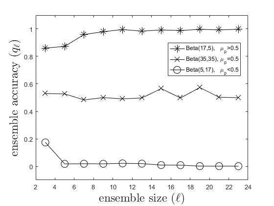
Figure 1: Convergence of ensemble accuracies for member accuracies coming from different Beta$(\alpha_{p},\beta_{p})$ distributions.

Now, to devise a stochastic model, we start with checking the possible distributions of the member accuracy values $p_{i}$ to estimate the ensemble accuracy. Then, we extend our model regarding this estimation by incorporating time information, as well. Notice that the estimation of the ensemble accuracy will be exploited to derive a stopping rule for the ensemble selection process.

4.1 Estimation of the distribution of member accuracies

Among the various possibilities, we have found that the beta distribution is a very good choice to analyze the distribution of member accuracies. The main reason is that beta concentrates on the interval $[0,1]$, that is, it can exactly capture the domain for the smallest/largest accuracy. Moreover, the beta distribution is able to provide density functions of various shapes that often appear in practice. Thus, to start the formal description, let the variate $p$ be distributed as Beta$\left(\alpha_{p},\beta_{p}\right)$ with density

$$b\left(x;\alpha_{p},\beta_{p}\right)=\frac{x^{\alpha_{p}-1}\left(1-x\right)^{\beta_{p}-1}}{B\left(\alpha_{p},\beta_{p}\right)},$$ (11)

where $B\left(\alpha_{p},\beta_{p}\right)=\Gamma\left(\alpha_{p}\right)\Gamma\left(\beta_{p}\right)/\Gamma\left(\alpha_{p}+\beta_{p}\right)$. In this case,

$$\mu_{p}=\alpha_{p}/\left(\alpha_{p}+\beta_{p}\right),$$ (12)

and $\mu_{p}\in\left(1/2,1\right)$ if and only if $\alpha_{p}>\beta_{p}$. If $\alpha_{p}=\beta_{p}$, then $\mu_{p}=1/2$. In the case of $\alpha_{p}>\beta_{p}$, the mode is also greater than $1/2$. The mode is infinite if $\beta_{p}<1$; therefore, we exclude this situation and we assume from now on that

$$1<\beta_{p}<\alpha_{p}.$$ (13)

The variance of $p$ is

$$\sigma^{2}_{p}=\frac{\alpha_{p}\beta_{p}}{\left(\alpha_{p}+\beta_{p}\right)^{2}\left(\alpha_{p}+\beta_{p}+1\right)}.$$ (14)

Since $\mu_{q_{\ell}}$, and $\sigma_{q_{\ell}}^{2}$ depend on $\mu_{p}$, and $\sigma^{2}_{p}$ according to (7) and (9) respectively, one can calculate both of them explicitly. The convergence of $\mu_{q_{\ell}}$ to 1 is fast if $\mu_{p}$ is close to $1$, i.e., $\beta_{p}\ll\alpha_{p}$; for instance, if $\alpha_{p}=17$, $\beta_{p}=5$. Simulations show that the speed of the convergence of $\sigma_{q_{\ell}}^{2}$ is exponential; hence, the usual square-root law does not provide the Central Limit Theorem for $q_{\ell}$.

In practice, we perform a beta fit on the $p_{i}$’s $(i=1,\dots,n)$. If a fit is found at least at the confidence level 0.95, we take the parameters $\alpha_{p},\beta_{p}$ provided by the fit and calculate $\mu_{p},\sigma^{2}_{p}$ by (12) and (14), respectively. If the beta fit is rejected, then $\mu_{p}$ and $\sigma^{2}_{p}$ are estimated from the $p_{i}$’s as the empirical mean and variance:

$$\mu_{p}=\frac{1}{n}\sum\limits_{i=1}^{n}p_{i},~{}\sigma^{2}_{p}=\frac{1}{n-1}\sum\limits_{i=1}^{n}(p_{i}-\mu_{p})^{2}.$$ (15)

To simplify our further notation we do not indicate whether the mean and variance have been estimated from the fitted distribution or empirically.

4.2 Adding time constraints to the model

Now, we turn to the case when together with the item accuracy $p_{i}$, we consider its running time $t_{i}$, as well. The common distribution of a random time is exponential, so let $\tau$ be an exponential distribution with density $\lambda\exp\left(-\lambda t\right)$. If $p$ is distributed as Beta$\left(\alpha_{p},\beta_{p}\right)$, then with setting $\lambda=1-p$ for a given $p$, the distribution of $\lambda$ becomes Beta$\left(\beta_{p},\alpha_{p}\right)$.

This is a reasonable behavior of time because it is quite natural to assume that more accurate components require more resources such as a larger amount of computation times. On the other hand, the selection procedure becomes trivial, if, e.g., the time and accuracy are not inversely proportional, since then the most accurate member is also the fastest one; therefore, it should be selected first by following this strategy for the remaining members until reaching the time limit. For some other possible simple accuracy–time relations, see our preliminary work [19].

For a given time constraint $T$, consider the random number $\ell_{T}$ such that

$$\sum_{j=0}^{\ell_{T}}\tau_{j}\leq T.$$ (16)

With the following lemma, our purpose is to provide an estimation $\widehat{{\ell}_{T}}$ for the expected size of the composed ensemble and incorporate this information in our stochastic characterization of $q_{\ell}$.

Lemma 4.2.

Let $\tau$ be an exponential distribution with density $\lambda\exp\left(-\lambda t\right)$ under the condition that the parameter $\lambda$ is distributed as Beta$\left(\beta_{p},\alpha_{p}\right)$, where $2<\beta_{p}<\alpha_{p}$.

1. Then, the expected time for the sum of $n$ variables is

   $$\sum_{k=0}^{n}E\tau_{k}=n\left(1+\frac{\alpha_{p}}{\beta_{p}-1}\right)$$ (17)

   with variance

   $$Var\left(\sum_{k=0}^{n}\tau_{k}\right)=n\left(1+\frac{\alpha_{p}}{\beta_{p}-2}\right).$$ (18)

   This implies that the estimated number of ensemble members up to time $T$ is $\widehat{\ell_{T}}=\left\lceil T\frac{\beta_{p}-1}{\alpha_{p}+\beta_{p}-1}\right\rceil.$

2. If the interarrival times $\tau_{j}$ correspond to a given $T$ and $\lambda$ generated from $\textsl{Beta}\left(\beta_{p},\alpha_{p}\right)$, then

   $$E(\ell_{T})=\frac{\beta_{p}}{\alpha_{p}+\beta_{p}}T.$$ (19)

3. If each component of pair $\left(\lambda_{j},\tau_{j}\right)$ are independent copies of $\lambda$ and $\tau_{j}$ corresponds to $\lambda_{j}$, then

   $$E(\ell_{T})=T\frac{\beta_{p}-1}{\alpha_{p}+\beta_{p}-1}.$$ (20)

In both cases 2) and 3), $\ell_{T}$ is distributed as Poisson with parameter $T/E\tau_{1}$, which implies that $Var\left(\ell_{T}\right)=E(\ell_{T})$ and the estimation of $\ell_{T}$ is

$$\widehat{{\ell}_{T}}=T/{\overline{\tau}}.$$ (21)

Proof.

See Appendix F for the proof. ∎

So far, we have assumed that $p$ is distributed as beta to calculate $\widehat{\ell_{T}}$ by Lemma 4.2. If this is not the case, we consider the following simple and obvious calculation for the approximate number of $\ell$ under the time constraint $T$:

$$\widehat{\ell_{T}}=\left\lceil nT\bigg{/}{\sum_{i=1}^{n}t_{i}}\right\rceil=\left\lceil T/{\overline{t}}\right\rceil;$$ (22)

another alternative to derive $\widehat{\ell_{T}}$ in this case is discussed in section 6. In either way it is derived, the value $\widehat{\ell_{T}}$ will be used in the stopping rule in our ensemble selection procedure; the proper details will be given next.

4.3 Stopping rule for ensemble selection

The procedure of finding $\left({\cal L}_{0},\ell_{0}\right)$ is a selection task that is NP-hard. We propose an algorithm such that we stop the selection when the value of $q_{\ell}\left({\cal L}\right)$ is sufficiently close to the possible maximum, which is not known. To be able to do so, we must give a proper stochastic characterization of $q_{\ell}$ by also settling on the calculation of $\mu_{q_{\ell}}$ and $\sigma^{2}_{q_{\ell}}$ via Lemma 4.1. First, notice that the values of $q_{\ell}\$are in $\left(0,1\right)$; indeed, it is positive and

$$\begin{split}q_{\ell}&=\sum_{k=\left\lfloor\frac{\ell}{2}\right\rfloor+1}^{\ell}\sum_{\begin{subarray}{c}I\subseteq{\cal N}\\ \left|I\right|=k\end{subarray}}{\displaystyle\prod\limits_{i\in I}}p_{i}{\displaystyle\prod\limits_{j\in{\cal N}\backslash I}}\left(1-p_{j}\right)\\ &<{\displaystyle\prod\limits_{j}}\left(p_{j}+\left(1-p_{j}\right)\right)=1.\end{split}$$ (23)

For the case when $p_{i}$’s are beta distributed, the product of independent beta variates can be close to beta again; see [22]. We have also performed MC simulation and found that beta distributions fit $q_{\ell}$ particularly well, compared to, e.g., the gamma, normal, Weibull, and extreme-valued distributions. Specifically, though the beta behavior of $q_{\ell}$ was naturally more stable for beta distributed $p_{i}$’s, the usual behavior of $q_{\ell}$ was also the same for non-beta $p_{i}$’s.

Thus, to provide a description of the stochastic behavior of $q$, we consider the following strategy. With a primary assumption on the $\emph{Beta}(\alpha_{q},\beta_{q})$ distribution of $q_{\ell}$, we calculate $\alpha_{q}$ and $\beta_{q}$ as

$$\begin{split}\alpha_{q}=\left(\frac{1-\mu_{q}}{\sigma_{q}^{2}}-\frac{1}{\mu_{q}}\right)\mu_{q}^{2},~{}~{}\beta_{q}=\alpha_{q}\left(\frac{1}{\mu_{q}}-1\right).\end{split}$$ (24)

If time information is provided for the pool items, we calculate $\widehat{\ell_{T}}$ by Lemma 4.2, and as a simpler notation, we will write $\widehat{\ell}$ from now on. If time information is not available, we will set $\widehat{\ell}=n$.

Next, we decide whether $q_{\ell}$ should be considered as beta with requiring $1<\beta_{q}<\alpha_{q}$ to be fulfilled to have a mode that is larger than 1/2 and finite. If this condition does not hold, we reject the beta behavior of $q_{\ell}$, and based on simulations, we characterize it as a normal distribution and stop the search if

$$q_{\ell}\geq\kappa_{0.9}\sigma_{q_{\widehat{\ell}}}/\sqrt{\widehat{\ell}}+\mu_{q_{\widehat{\ell}}}=STOP,$$ (25)

where $\kappa_{0.9}$ is the 0.9 quantile of the standard normal distribution. Otherwise, when $q_{\ell}$ is considered beta, we calculate the mode $\nu$ of Beta($\alpha_{q}$, $\beta_{q}$) for $q_{\ell}$ as

$$\nu=\frac{\alpha_{q}-1}{\alpha_{q}+\beta_{q}-2},$$ (26)

and the Pearson’s first skewness coefficient as

$$\gamma=\frac{1-\nu}{{\sigma_{q_{\widehat{\ell}}}}}.$$ (27)

Then, we use Table I to select the appropriate probability value $\varrho_{q_{\widehat{\ell}}}$; the entries are determined by simulation in the case of $2\leq\beta_{q}<\alpha_{q}$.

We stop the selection when the ensemble accuracy reaches the value of the inverse cumulative distribution $F_{\alpha_{q},\beta_{q}}^{-1}(\varrho_{q_{\widehat{\ell}}})$ of $\emph{Beta}(\alpha_{q},\beta_{q})$ in the given probability, that is, when

$$q_{\ell}\geq F_{\alpha_{q},\beta_{q}}^{-1}(\varrho_{q_{\widehat{\ell}}})=STOP.$$ (28)

TABLE I: Probability values $\varrho_{q_{\widehat{\ell}}}$ for stopping thresholds for different skewness coefficients $\gamma$.

$\gamma$	$\varrho_{q_{\widehat{\ell}}}$
$\gamma\leq 1$	$0.6$
$1<\gamma\leq 2.5$	$0.8$
$2.5<\gamma\leq 3.5$	$0.9$
$3.5<\gamma$	$0.95$

In either via (25) or (28), an estimation for the ensemble accuracy is gained; we obtain a STOP value to stop the stochastic search. However, there is some chance that STOP is not exceeded, though in our experiments it has never occurred. Thus, to avoid an infinite loop, we consider a maximum allowed step number MAXSTEP as an escaping stopping rule. Namely, to obtain MAXSTEP, we apply Stirling’s approximation

$$\mbox{MAXSTEP}=\binom{n}{\widehat{\ell}}\sim n^{\widehat{\ell}}/{\widehat{\ell}!},$$ (29)

assuming that $\widehat{\ell}/n\rightarrow 0$. This is a reasonable approach since $\widehat{\ell}$ is calculated according to Lemma 4.2 or (22). The formal description of our proposed ensemble selection method is enclosed in Algorithm 2.

Algorithm 2 Proposed Ensemble Creation Method.

1:[NO-TIME]: Pool $\mathcal{D}=\left\{p_{i}\right\}_{i=1}^{n}$.  

2:[TIME]:

Pool $\mathcal{D}=\left\{\left(p_{i},t_{i}\right)\right\}_{i=1}^{n}$,

Total allowed time $T$.

 

3:An ensemble $\mbox{MAXENS}\subseteq\mathcal{D}$ to maximize system accuracy (1) within time $T$ as in (2).  

4:Calculate the mean $\mu_{p}$ and std $\sigma_{p}$ for $\{p_{i}\}_{i=1}^{n}$

5:         by (12) and (14) (if a beta fits to $p$) or

6:         empirically (if $p$ is not beta) by (15)

7:switch Input do

8:   case NO-TIME

9:      $\widehat{\ell}\leftarrow n$    

10:   case TIME

11:      Estimate # of members $\widehat{\ell}$ for $T$ by

12:         Lemma 4.2 if a beta fits to $p$, or by (22)

13:         if $p$ is not beta    

14:Calculate $\mu_{q_{\widehat{\ell}}}$ by (7) and $\sigma^{2}_{q_{\widehat{\ell}}}$ by (9)

15:Calculate $\alpha_{q}$, $\beta_{q}$ by (24)

16:if $1<\beta_{q}<\alpha_{q}$ then

17:   Calculate cdf. $F_{\alpha_{q},\beta_{q}}$, $\nu$, $\gamma$, $\varrho_{q_{\widehat{\ell}}}$ by (26), (27)

18:         and Table I, and adjust STOP with (28)

19:else

20:   Adjust STOP with (25)

21:end if

22:Calculate MAXSTEP by (29)

23:switch Input do

24:   case NO-TIME

25:      Compose ensemble by SA using STOP

26:         and MAXSTEP for the stopping rule    

27:   case TIME

28:      Compose ensemble either by Algorithm 1

29:         (SHErLoCk) or SA using STOP and

30:         MAXSTEP for the stopping rule    

Before providing our detailed empirical results in section 5, in Table II we summarize our findings for Algorithm 2 on simulations. Namely, in two respective tests with $i=1,\dots,30$ and $i=1,\dots,100$, we have generated the $p_{i}$’s to come from $\emph{Beta}(17,5)$ and the execution times $t_{i}$ from conditional exponential distributions with parameters $\lambda=1-p_{i}$. The time constraint $T$ was set in seconds to $30\%$ of the total time $\sum_{i=1}^{30}t_{i}$ for the first, and $20\%$ of $\sum_{i=1}^{100}t_{i}$ for the second test. Both tests were repeated 100 times, and we have taken the averages of the obtained precisions. As our primary aim, we have checked whether the stopping rule of the stochastic search indeed led to a reasonable computational gain. For the sake of completeness, in Table II we have also shown the results regarding letting the search continue in the long run (stopped by MAXSTEP), though in each of our tests, the STOP value has been exceeded much earlier. Secondarily, we have compared SA with our selection method SHErLoCk given in Algorithm 1. For Table II, we can conclude that applying our stopping rule by using STOP saved considerable computational time compared with the exhaustive search that culminated by stopping it with MAXSTEP with a negligible drop in accuracy. Moreover, our approach has found efficient ensembles quicker than SA. These impressions have also been confirmed by the empirical evaluations on real data described in the next section.

TABLE II: Result of Algorithm 2 on simulations.

Search	Ensemble accuracy		Comp. time (secs)
method	MAXSTEP	STOP	MAXSTEP	STOP
SHErLoCk ($n$=30)	$99.56\%$	$99.39\%$	$60.03$	$0.08$
SA ($n$=30)	$98.97\%$	$98.91\%$	$87.40$	$0.30$
SHErLoCk ($n$=100)	$99.66\%$	$99.61\%$	$294.58$	$1.54$
SA ($n$=100)	$99.38\%$	$99.37\%$	$638.39$	$1.58$

5 Empirical analysis

In this section, we demonstrate the efficiency of our models through an exhaustive experimental test on publicly available data. Our first experiment considers the possibility of organizing competing approaches with different accuracies into an ensemble. In this scenario, accuracy values correspond to final scores of participants of Kaggle challenges without cost/time information provided. Our second setup for ensemble creation considers machine learning-based binary classifiers as possible members; the performance evaluation is performed on several UCI Machine Learning Repository [23] datasets with the training times considered as costs.

5.1 Kaggle challenges

Kaggle is an open online platform for predictive modeling and analytics competitions with the aim of solving real-world machine learning problems provided by companies or users. The main idea behind this crowd-sourcing approach is that a countless number of different strategies might exist to solve a specific task, and it is not possible to know beforehand which one is the most effective. Though primarily only the scores of the participating algorithms can be gathered from the Kaggle site, as a possible future direction, we are curious regarding whether creating ensembles from the various strategies could lead to an improvement regarding the desired task.

Not all the Kaggle competitions are suitable to test our models since in the current content, we focus on majority voting-based ensemble creation. Consequently, we have collected only such competitions and corresponding scores where majority voting-based aggregation could take place. More precisely, we have restricted our focus only to such competition metrics based on which majority voting can be realized. Such metrics include quadratic weighted kappa, area under the ROC curve (AUC), log loss, normalized Gini coefficient. For concrete competitions where these metrics were applied, we analyze the following ones: Diabetic Retinopathy Detection, DonorsChoose.org Application Screening , Statoil/C-CORE Iceberg Classifier Challenge, WSDM - KKBox’s Churn Prediction Challenge, and Porto Seguro’s Safe Driver Prediction.

For our analytics, on the one hand it is interesting to observe the distribution of the final score of the competitors, which is often affected by the volume of the prize money offered to the winner. Moreover, accuracy measurement is usually scaled to the interval $[0,1]$, with 0 for the worst and 1 for the perfect performance, which allows us to test our results regarding the beta distributions. As a drawback of Kaggle data, access to the resource constraints corresponding to the competing algorithms (e.g., training/execution times) is rather limited; such data are provided for only a few competitions, primarily in terms of execution time interval.

Thus, to summarize our experimental setup, we interpret the competing solutions of a Kaggle challenge as the $\{D_{1},D_{2},\dots,D_{n}\}$ pool, where the score of $D_{i}$ is used for the accuracy term $p_{i}\in[0,1]$ in our model. Then, we apply a beta fit for each investigated challenge to determine whether a beta distribution fits the corresponding scores or not. If the test is rejected, we can still use the estimation for the joint behavior $q$ using (15) and (22). If the beta test is accepted, we can also apply our corresponding results using (12), (14), and Lemma 4.2. Notice that reliably fitting a model for the scores of the competitors might lead to a better insight of the true behavior of the data of the given field, also for the established expectations there.

As observed from Table III, SA was able to stop much earlier with a slight loss in accuracy using the suggested stopping rule (STOP) in finding the optimal ensemble. Our approach SHErLoCk given in Algorithm 1 has been excluded from this analysis since no cost information was available.

TABLE III: Ensemble accuracies on the Kaggle datasets found by simulated annealing (SA).

Dataset	Ensemble accuracy		Computational time (secs)
Name	MAXSTEP	STOP	MAXSTEP	STOP
Diabetic Retinopathy Detection	94.34%	93.19%	194.12	1.31
DonorsChoose.org Application Screening	94.78%	91.96%	206.89	1.67
Statoil/C-CORE Iceberg Classifier Challenge	88.42%	87.76%	191.91	2.23
WSDM - KKBox’s Churn Prediction Challenge	96.96%	96.32%	203.88	1.45
Porto Seguro’s Safe Driver Prediction	92.99%	89.98%	214.28	1.95
Average	92.29%	90.45%	202.21	1.72

5.2 Binary classification problems

The UCI Machine Learning Repository [23] is a popular platform to test the performances of machine learning-based approaches, primarily for classification purposes. A large number of datasets are made publicly available here among which our models can be tested on binary classification ones. That is, in this experiment, the members $D_{1},D_{2},\dots,D_{n}$ of a pool for ensemble creation are interpreted as binary classifiers, whose outputs can be aggregated by the majority voting rule. Using the ground truth supplied with the datasets, the accuracy term $p_{i}\in[0,1]$ stands for the classification accuracy of $D_{i}$.

The number of commonly applied classifiers is relatively low; therefore to increase the cardinality of the pool, we have also considered a synthetic approach in a similar way to [24]. Namely, we have trained the same base classifier on different training datasets, by which we can synthesize several ”different” classifiers. Naturally, this method is able to provide more independent classifiers only if the base classifier is unstable, i.e., minor changes in the training set can lead to major changes in the classifier output; such an unstable classifier is, for example, the perceptron one.

To summarize our experimental setup for UCI binary classification problems, we have considered base classifiers perceptron [25], decision tree [26], Levenberg-Marquardt feedforward neural network [27], random neural network[28], and discriminative restricted Boltzmann machine classifier [29] for the datasets MAGIC Gamma Telescope [30], HIGGS [31], EEG Eye State [23], Musk (Version 2) [32], and Spambase [23]; datasets of large cardinalities were selected to be able to train synthetic variants of base classifiers on different subsets. To check our models for different numbers of possible ensemble members, the respective pool sizes were set to $n=30$ and $n=100$; the necessary number of classifiers has been reached via synthesizing the base classifiers with training them on different subsets of the training part of the given datasets. In contrast to the Kaggle challenges, in these experiments we were able to retrieve meaningful cost information to devise a knapsack scenario. Namely, for a classifier $D_{i}$, its training time was adjusted as its cost $t_{i}$ in our model. Notice that for even the same classifier, it was possible to obtain different $t_{i}$ values with training its synthetic variants on datasets of different sizes. Using this time information, for the estimated size $\widehat{\ell}$ of the optimal ensemble, we could use Lemma 4.2 for $n=30$, while (22) for the case $n=100$.

As clearly visible from Tables IV and V, our stochastic search strategy SHErLoCk described in Algorithm 1 was reasonably faster than SA and slightly dominant in accuracy, as well. Moreover, it can be observed again that applying the stopping rule with the threshold STOP led to an enormous computational advantage for either search strategies with only a small drop in accuracy.

TABLE IV: Comparing simulated annealing (SA) with the proposed search strategy (SHErLoCk) on binary classification problems of UCI datasets using an ensemble pool of $n=30$ classifiers.

Dataset		Ensemble accuracy				Computational time (secs)
Name	Size	MAXSTEP		STOP		MAXSTEP		STOP
		SA	SHErLoCk	SA	SHErLoCk	SA	SHErLoCk	SA	SHErLoCk
MAGIC	19 020	99.34%	99.57%	99.17%	99.29%	171.9	56.47	0.41	0.18
Spambase	4 601	99.68%	99.76%	98.95%	98.77%	100.98	67.90	1.67	0.39
HIGGS	20 000	78.03%	77.99%	77.59%	77.63%	158.90	69.46	2.73	0.93
EEG	14 980	98.71%	98.80%	95.62%	97.43%	345.57	90.20	0.47	0.38
Musk	6 598	99.95%	99.99%	99.96%	99.98%	178.21	58.89	0.33	0.32
Average		95.15%	95.07%	94.26%	94.62%	191.11	68.06	1.12	0.44

TABLE V: Comparing simulated annealing (SA) with the proposed search strategy on binary classification problems of UCI datasets using an ensemble pool of $n=100$ classifiers.

Dataset		Ensemble accuracy				Computational time (secs)
Name	Size	MAXSTEP		STOP		MAXSTEP		STOP
		SA	SHErLoCk	SA	SHErLoCk	SA	SHErLoCk	SA	SHErLoCk
MAGIC	19 020	99.57%	99.59%	99.19%	99.34%	349.62	194.12	1.31	1.32
Spambase	4 601	99.79%	99.78%	98.96%	98.88%	390.89	206.89	1.67	1.41
HIGGS	20 000	78.08%	78.16%	77.79%	77.73%	378.56	191.91	2.23	2.11
EEG	14 980	98.96%	98.96%	97.32%	97.64%	453.59	203.88	1.45	1.33
Musk	6 598	99.98%	99.99%	99.98%	99.98%	475.71	214.28	1.95	1.56
Average		95.28%	95.29%	94.65%	94.71%	409.67	202.21	1.72	1.55

5.3 Optic disc detection

The majority voting rule can be applied in a problem to aggregate the outputs of single object detectors in the spatial domain [13]; the votes of the members are given in terms of single pixels as candidates for the centroid of the desired object. In this extension, the shape of the desired object defines a geometric constraint, which should be met by the votes that can be aggregated. In [13], our practical example relates to the detection of a disc-like anatomical component, namely the optic disc (OD) in retinal images. Here, the votes are required to fall inside a disc of diameter $d_{OD}$ to vote together. As more false regions are possible to be formed, the correct decision can be made even if the true votes are not in the majority, as in Figure 2. The geometric restriction transforms (1) to the following form:

$$q_{\ell}({\cal L})=\sum\limits_{k=0}^{\ell}p_{\ell,k}\left({\underset{|{\cal I}|=k}{\sum\limits_{\cal I\subseteq{\cal L}}}}\prod\limits_{i\in\cal I}p_{i}\prod\limits_{j\in{\cal L}\setminus\cal I}\left(1-p_{j}\right)\right).$$ (30)

In (30), the terms $p_{\ell,k}$ describe the probability that a correct decision is made by supposing that we have $k$ correct votes out of $\ell$. For the terms $p_{\ell,k}$ $(k=0,1,\dots,\ell)$, in general, we have that $0\leq p_{\ell,0}\leq p_{\ell,1}\leq\dots\leq p_{\ell,\ell}\leq 1$.

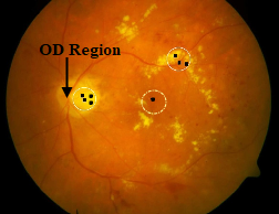
Figure 2: Successful OD detection with the same number of correct/false ensemble member responses.

In our experiments, the pool consists of eight OD detector algorithms with the following accuracy and running time values: $\{(p_{i},t_{i})\}_{i=1}^{8}=\{(0.220,31),(0.304,38),(0.319,34),(0.643,69),\\ (0.754,11),(0.765,7),(0.958,21),(0.976,90)\}$ with $\sum_{i=1}^{8}t_{i}=301$ secs. We can apply our theoretical foundation with some slight modifications to solve the same kind of knapsack problem for the variant (30), transforming the model to reflect the multiplication with the terms $p_{\ell,k}$.

We have empirically derived the values $p_{8,k}=\{0,0.11,0.70,0.93,0.99,1.00,1.00,1.00,1.00\}$ for (30) in our task. To adopt our approach by following the logic of Algorithm 2, we need to determine a STOP value for the search based on $\mu_{p}$ and $\sigma_{p}$ (calculated by (15)), and $\widehat{\ell}$ (calculated by (22)). However, since now the energy function is transformed by the terms $p_{\ell,k}$ in (30), we must borrow the corresponding theoretical results from [33] to derive the mean $\mu_{q_{\widehat{\ell}}}$ instead of (7) proposed in Algorithm 2. Accordingly, we had to find a continuous function $\cal F$ that fit to the values $p_{\ell,k}$, which was evaluated by regression and resulted in ${\cal F}(x)={b}/({b+{x}^{a}/({1-x})^{a}})$ with $a=-3.43$ and $b=101.7$, as also plotted in Figure 3. Now, by using Theorem 1 from [33], we have gained $\mu_{q_{\widehat{\ell}}}={\cal F}(\mu_{p})$.

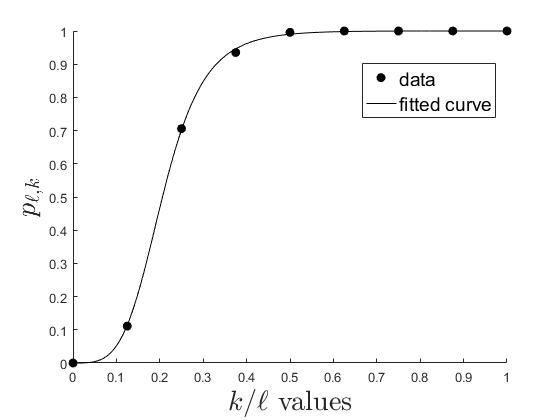
Figure 3: Determining the constrained majority voting probabilities $p_{\ell,k}$ for our OD detector ensemble.

For our experiment to search for the best ensemble, we have set the time constraint to be 80% of the total running time, with $T=4(\sum_{i=1}^{8}t_{i})/5$. For this setup, we could estimate $\widehat{\ell}=7$ and $\mu_{q_{\widehat{\ell}}}=0.969$ for the expected ensemble size and mean accuracy, respectively. Then, these values have been considered for Algorithm 2 to compare the performance of our stochastic search method SHErLoCk with SA. As shown in Table VI, our search strategy outperformed SA also for the object detection problem both in accuracy and computational time.

TABLE VI: Comparing SA with the proposed search strategy SHErLoCk on the OD detection problem.

Search	Ensemble accuracy	Comp. time (secs)
method	STOP	STOP
SHErLoCk	$99.45\%$	$0.07$
SA	$99.43\%$	$0.16$

6 Discussion

For the approximate number $\widehat{{\ell}_{T}}$ of the ensemble size, we have considered (22) when the member accuracy $p$ is not a beta distribution. As an alternative, notice that it is known that for a given $\lambda$, $T$ and an independent exponential distributed $\tau_{j}$, $\ell_{T}$ is distributed as Poisson with parameter $\lambda T$. We can use Lemma 4.2 and conclude that for a starting size of the ensemble, one may choose $\widehat{{\ell}_{T}}$ such that the remaining possible values are beyond the 5% error. It follows that we apply formula either

$$\textrm{P}\left(\ell_{T}>m_{0.05}\right)=0.05,$$ (31)

where $m_{0.05}$ is the upper quantile of the Poisson distribution with parameter $T/\sum_{i=1}^{n}p_{i}$, or use the normal approximation to the Poisson distribution

$$\frac{\ell_{T}-T/\sum_{i=1}^{n}p_{i}-0.5}{\sqrt{T/\sum_{i=1}^{n}t_{i}}}>1.64,$$ (32)

which provides us the inequality

$$\ell_{T}>\frac{T}{\sum_{i=1}^{n}t_{i}}+0.5+1.64\sqrt{\frac{T}{\sum_{i=1}^{n}t_{i}}}=\widehat{\ell_{T}}.$$ (33)

In our experiments we have used (22) instead of (33) to obtain $\widehat{\ell_{T}}$, since the latter provided slightly too large estimated size values. However, for other scenarios, it might be worthwhile to try (33), as well.

As some additional arguments, we call attention to the following issues regarding those elements of our approach that might need special care or can be adjusted differently in other scenarios:

• We have assumed independent member accuracy behavior, providing solid estimation power in our tests. However, in the case of strong member dependencies, deeper discovery of the joint behavior might be needed.

• Stirling’s approximation considered in (29) may provide values that are too small for the parameter MAXSTEP in the case of small pools. Since this is an escape parameter, a sufficiently large value should be selected in such cases instead.

• The time profile $\lambda=1-p$ considered in section 4.2 is suited to our data; however, any other relationship between the member accuracy and time can be considered. Nevertheless, the proper derivation of the estimation of the ensemble accuracy might be slightly more laborious.

• In (25), we have used a one-tailed (left-side) hypothesis since $q_{\ell}$ was close to 1. However, if it is not that close to 1, a two-tailed hypothesis can be meaningful, as well. Furthermore, if $\mu_{q}$ is even smaller (say 0.7), then we can search above this mean by considering a right-side hypothesis.

Appendices

Appendix A Proof for Lemma 1.1.

Proof.

Consider a subset $\mathcal{K}$ when $\mathcal{K}=\left\{1,2,\ldots,2\ell\right\}$ (otherwise we can renumerate $p_{i}$). We have

$$q_{2\ell}\left(\mathcal{K}\right)=\sum_{k=\ell+1}^{2\ell}\sum_{\begin{subarray}{c}I\subseteq\mathcal{K}\\ \left|I\right|=k\end{subarray}}{\displaystyle\prod\limits_{i\in I}}p_{i}{\displaystyle\prod\limits_{j\in\mathcal{K}\backslash I}}\left(1-p_{j}\right)\\ =\sum_{k=\ell+1}^{2\ell}\sum_{\begin{subarray}{c}I\subseteq\mathcal{K}\\ \left|I\right|=k\end{subarray}}Q_{2\ell,k}\left(\mathcal{K},I\right),$$ (34)

where

$$Q_{2\ell,k}\left(\mathcal{K},I\right)={\displaystyle\prod\limits_{i\in I}}p_{i}{\displaystyle\prod\limits_{j\in\mathcal{K}\backslash I}}\left(1-p_{j}\right),$$ (35)

that is, we consider a subset $\mathcal{K}\subseteq\mathcal{N}$ with $\left|\mathcal{K}\right|=2\ell$, and $Q_{2\ell,k}\left(\mathcal{K},I\right)$ is calculated for an index set $I\subseteq\mathcal{K}$ with $\left|I\right|=k$. Now, choose an index $a$ from the set $\mathcal{N}\backslash\mathcal{K}$, i.e., $a>2\ell$, and obtain

$$Q_{2\ell,k}\left(\mathcal{K},I\right)=Q_{2\ell,k}\left(\mathcal{K},I\right)p_{a}+Q_{2\ell,k}\left(\mathcal{K},I\right)\left(1-p_{a}\right).$$ (36)

The term $Q_{2\ell,k}\left(\mathcal{K},I\right)p_{a}=Q_{2\ell+1,k+1}\left(\left\{\mathcal{K},a\right\},\left\{I,a\right\}\right)$ and $\ Q_{2\ell,k}\left(\mathcal{K},I\right)\left(1-p_{a}\right)=Q_{2\ell+1,k}\left(\left\{\mathcal{K},a\right\},I\right)$; therefore,

$$q_{2\ell}\left({\cal{K}}\right)=\sum_{k=\ell+1}^{2\ell}\sum_{\begin{subarray}{c}I\subseteq{\cal{K}}\\ \left|I\right|=k\end{subarray}}Q_{2\ell,k}\left({\cal{K}},I\right)\\ =\sum_{k=\ell+1}^{2\ell}\left(\sum_{\begin{subarray}{c}I\subseteq{\cal{K}}\\ \left|I\right|=k\end{subarray}}Q_{2\ell+1,k+1}\left(\left\{{\cal{K}},a\right\},\left\{I,a\right\}\right)+\right.\\ \left.+\sum_{\begin{subarray}{c}I\subseteq{\cal{K}}\\ \left|I\right|=k\end{subarray}}Q_{2\ell+1,k}\left(\left\{{\cal{K}},a\right\},I\right)\right)\\ <\sum_{k=\ell+1}^{2\ell}\sum_{\begin{subarray}{c}I\subseteq{\cal{K}}\\ \left|I\right|=k\end{subarray}}Q_{2\ell+1,k}\left({\cal{K}},I\right)=q_{2\ell+1}\left({\cal{K}},a\right),$$ (37)

since $q_{2\ell+1}\left(\mathcal{K}\right)$ includes some extra additional terms, say $Q_{2\ell+1,k}\left(\left\{\mathcal{K},a\right\},I\right)$, where $I$ contains $a$. Regarding that $n$ is odd in the series of $q_{\ell}\left(\mathcal{K}\right)$, there will be an element with odd $\ell$ following an element of even $\ell$ and the lemma is proved for odd $n$. For the case when $n$ is even, we consider the $q_{n}\left(\mathcal{N}\right)$ and $q_{n-1}\left(\mathcal{L}\right)$, where $\mathcal{L}=\left\{1,2,\ldots,2\ell-1\right\}$. Set $n=2\ell$; then,

$$q_{2\ell}\left(\mathcal{N}\right)=\sum_{k=\ell+1}^{2\ell}\sum_{\begin{subarray}{c}I\subseteq\mathcal{N}\\ \left|I\right|=k\end{subarray}}Q_{2\ell,k}\left(\mathcal{N},I\right)$$ (38)

with $\mathcal{N}=\ \left\{1,2,\ldots,2\ell\right\}$ and put

$$q_{2\ell-1}\left(\mathcal{L}\right)=\sum_{k=\ell}^{2\ell-1}\sum_{\begin{subarray}{c}I\subseteq\mathcal{L}\\ \left|I\right|=k\end{subarray}}Q_{2\ell-1,k}\left(\mathcal{L},I\right),$$ (39)

notice that the number of terms is equal in both sums. If $k=2\ell$, then

$$Q_{2\ell,2\ell}\left(\mathcal{N},\mathcal{N}\right)=p_{2\ell}Q_{2\ell-1,2\ell-1}\left(\mathcal{L},\mathcal{L}\right),$$ (40)

otherwise,

$$Q_{2\ell,k}\left(\mathcal{N},I\right)=\left\{\begin{array}[c]{ccc}p_{2\ell}Q_{2\ell-1,k-1}\left(\mathcal{L},I\backslash 2\ell\right)&\text{if}&2\ell\in I\\ \left(1-p_{2\ell}\right)Q_{2\ell-1,k}\left(\mathcal{L},I\right)&\text{if }&2\ell\notin I\end{array}\right.,$$ (41)

hence for $k<2\ell$,

$$\sum_{\begin{subarray}{c}I\subseteq\mathcal{N}\\ \left|I\right|=k\end{subarray}}Q_{2\ell,k}\left(\mathcal{N},I\right) =p_{2\ell}\sum_{\begin{subarray}{c}I\subseteq\mathcal{L}\\ \left|I\right|=k-1\end{subarray}}Q_{2\ell-1,k-1}\left(\mathcal{L},I\right)$$

$$+\left(1-p_{2\ell}\right)\sum_{\begin{subarray}{c}I\subseteq\mathcal{L}\\ \left|I\right|=k\end{subarray}}Q_{2\ell-1,k}\left(\mathcal{L},I\right).$$ (42)

We start summing up $q\left(\mathcal{N},2\ell\right)$ from $2\ell$; then, using (40) and (A), we obtain for the first two terms

$$\sum_{k=2\ell-1}^{2\ell}\sum_{\begin{subarray}{c}I\subseteq\mathcal{N}\\ \left|I\right|=2\ell-1\end{subarray}}Q_{2\ell,k}\left(\mathcal{N},I\right)=p_{2\ell}Q_{2\ell-1,2\ell-1}\left(\mathcal{L},\mathcal{L}\right)\\ +p_{2\ell}\sum_{\begin{subarray}{c}I\subseteq\mathcal{L}\\ \left|I\right|=2\ell-2\end{subarray}}Q_{2\ell-1,2\ell-2}\left(\mathcal{L},I\right)+\left(1-p_{2\ell}\right)Q_{2\ell-1,2\ell-1}\left(\mathcal{L},\mathcal{L}\right)\\ =Q_{2\ell-1,2\ell-1}\left(\mathcal{L},\mathcal{L}\right)+p_{2\ell}\sum_{\begin{subarray}{c}I\subseteq\mathcal{L}\\ \left|I\right|=2\ell-2\end{subarray}}Q_{2\ell-1,2\ell-2}\left(\mathcal{L},I\right).$$ (43)

If we continue summing up one by one, then induction leads to

$$q_{2\ell}\left(\mathcal{N}\right)=\sum_{k=\ell+1}^{2\ell-1}\sum_{\begin{subarray}{c}I\subseteq\mathcal{L}\\ \left|I\right|=k\end{subarray}}Q_{2\ell-1,k-1}\left(\mathcal{L},I\right)\\ +p_{2\ell}\sum_{\begin{subarray}{c}I\subseteq\mathcal{L}\\ \left|I\right|=\ell\end{subarray}}Q_{2\ell-1,\ell}\left(\mathcal{L},I\right)<q_{2\ell-1}\left(\mathcal{L}\right),$$ (44)

since $p_{2\ell}<1$. ∎

Appendix B Proof for Proposition 2.1.

Proof.

We prove the statement with an example describing the worst-case scenario for the greedy selection strategy. Let ${\cal{D}}=\{D_{1}=(p_{1},t_{1}),D_{2}=(p_{2},t_{2}),\dots,D_{n}=(p_{n},t_{n})\}$ be the pool, where the index set is denoted by ${\cal{I}}_{n}=\{1,2,\ldots,n\}$. Let us suppose that $\sum\limits_{i=1}^{n}t_{i}\leq T$, that is, the time constraint should not be of concern. Let $p_{1}=1/2+\varepsilon$, where $0<\varepsilon\leq 1/2$, and $p_{2}=p_{3}=\dots=p_{n}=1/2+\alpha$ with $0<\alpha<\varepsilon$, where the proper selection of $\alpha$ will be given below.

The greedy strategy will move $D_{1}$ to $S$ as the most accurate item in its first step. Next, we try to extend $S$ by adding more members. Since we require odd members, we try to add 2 items in every selection step. Since all the remaining $n-1$ features have the same behavior, we can check whether $S$ should be extended via comparing the performance of $S_{1}=\{D_{1}\}$ and $S_{3}=\{D_{1},D_{2},D_{3}\}$. For the performance of the ensemble $S_{1}$, we trivially have $q_{1}({\cal{I}}_{1})=p_{1}=1/2+\varepsilon$, where ${\cal{I}}_{1}=\{1\}$, while for $S_{3}$ we can apply (1) for the 3-member ensemble, with ${\cal{I}}_{3}=\{1,2,3\}$ to calculate $q_{3}({\cal{I}}_{3})$:

$$q_{3}({\cal{I}}_{3}) = p_{1}p_{2}(1-p_{3})+p_{2}p_{3}(1-p_{1})+p_{1}p_{3}(1-p_{2})$$ (45)

$$+ p_{1}p_{2}p_{3}=\frac{1}{2}+\frac{\varepsilon}{2}+\alpha-2\alpha^{2}\varepsilon$$

after the appropriate substitutions and simplifications. Now, if we adjust $\alpha$ to have $q_{1}({\cal{I}}_{1})=q_{3}({\cal{I}}_{3})$, then via solving the equation

$$\frac{1}{2}+\varepsilon=\frac{1}{2}+\frac{\varepsilon}{2}+\alpha-2\alpha^{2}\varepsilon$$ (46)

we obtain

$$\alpha=\frac{1-\sqrt{1-4\varepsilon^{2}}}{4\varepsilon}.$$ (47)

That is, with a selection of $\alpha$ given in (47), the ensemble $S_{1}=\{D_{1}\}$ is not going to be extended since it does not lead to improvement. Thus, the strategy stops after the first step with an ensemble accuracy $1/2+\varepsilon$.

On the other hand, with a sufficiently large $n$, a very accurate ensemble could be achieved. More precisely, it can be easily seen that $q_{n}({\cal{I}}_{n})$ is strictly monotonically increasing with

$$\lim_{n\rightarrow\infty}q_{n}({\cal{I}}_{n})=1.$$ (48)

Now, by letting $\varepsilon\rightarrow 0$, we can see that for the ensemble accuracy found with this strategy

$$\lim_{\varepsilon\rightarrow 0}q_{1}(S_{1})=1/2,$$ (49)

while an ensemble of $\lim\limits_{n\rightarrow\infty}q_{n}({\cal{I}}_{n})=1$ could also be found. Hence, the proposition follows. ∎

Appendix C Proof for Proposition 2.2.

Proof.

We prove the statement with a similar example to that given in the proof of Proposition 2.1 in Appendix B to describe the worst case scenario. Let ${\cal{D}}=\{D_{1}=(p_{1},t_{1}),D_{2}=(p_{2},t_{2}),\dots,D_{n}=(p_{n},t_{n})\}$ be the pool and $T$ be the time constraint. Put $p_{1}=1/2+\varepsilon$, where $0<\varepsilon\leq 1/2$, $t_{1}=T$, and $p_{2}=p_{3}=\dots=p_{m}=1/2+\alpha$, $t_{2}=t_{3}=\dots=t_{n}=\displaystyle{T}/({n-1})$ with $0<\alpha<\varepsilon$. If $\alpha$ is properly selected, then $q_{1}({\cal{I}}_{1})=p_{1}<q_{n-1}({\cal{I}}_{n}\setminus{\cal{I}}_{1})$. However, because of the time constraint, we must remove elements during the selection procedure, since initially $\sum\limits_{i=1}^{n}t_{i}=2T>T$. For this requirement, the greedy approach in the first step will remove any two elements from $D_{2},\dots,D_{n}$ by decreasing the time with $\displaystyle{2T}/({n-1})$. This selection will go on until only $D_{1}$ remains in the ensemble. With a proper selection of $\alpha$, we have $\lim\limits_{n\rightarrow\infty}q_{n-1}({\cal{I}}_{n}\setminus{\cal{I}}_{1})=1$ and by letting $\varepsilon\rightarrow 0$, the proposition follows. ∎

Appendix D Proof for Proposition 2.3.

Proof.

Similar to the proof of Proposition 2.2, we provide an example for the worst case scenario. Let $D_{1}=(1,T)$, and $D_{2}=D_{3}=D_{4}=(1/2+\varepsilon,T/3)$ with $0<\varepsilon<1/2$. Now, since

$$u_{1}=\frac{1}{T}<\frac{3/2+3\varepsilon}{T}=u_{2}=u_{3}=u_{4},$$ (50)

the backward strategy will remove the less useful component $D_{1}$ first to maintain the time constraint and will keep the remaining ensemble $\{D_{2},D_{3},D_{4}\}$ as the most accurate one, which also fits the time constraint with $\sum\limits_{i=2}^{4}t_{i}=T$. By letting $\varepsilon\to 0$, we have $\lim_{\varepsilon\to 0}q_{3}({\cal{I}}_{4}\setminus{\cal{I}}_{1})=1/2$. Moreover, notice that the most accurate ensemble would have been $\{D_{1}\}$ with $q_{1}({\cal{I}}_{1})=1$ by meeting the time constraint, as well. Thus, the statement follows. ∎

Appendix E Proof for Lemma 4.1

Proof.

The first part of the lemma corresponds to Theorem 1 in [1]. For the rest, let us denote the product of probabilities by

$$\Pi\left(I\right)={\displaystyle\prod\limits_{i\in I}}p_{i}{\displaystyle\prod\limits_{j\in{\cal{N}}\backslash I}}\left(1-p_{j}\right),$$ (51)

for simplifying the treatment below. The formula (9) follows from expressing the variance in terms of covariance

$$\operatorname*{Var}\left(q_{\ell}\right)=\sum_{k,j=k_{\ell}}^{\ell}\sum_{\begin{subarray}{c}I,J\subseteq{\cal{N}}\\ \left|I\right|=k,\left|J\right|=j\end{subarray}}\operatorname*{Cov}\left(\Pi\left(I\right),\Pi\left(J\right)\right).$$ (52)

Now, we rewrite this expression into a more appropriate form. First, the notation is introduced, where $I_{T}^{k}\$and $I_{F}^{k}$ for a partition of indices ${\cal{N}}=\{1,\ldots,\ell\}$, such that ${\cal{N}}=I_{T}^{k}\cup I_{F}^{k}$ where $I_{T}^{k}$ denotes indices of those members voting true with accuracy $p$. Similarly, $I_{F}^{k}$ contains indices of false votes. Observe $I_{F}^{k}={\cal{N}}\backslash I_{T}^{k}$. We have $\left|I_{T}^{k}\right|=k$ and $\left|I_{F}^{k}\right|=\ell-k$. In the case of two partitions $I_{T}^{k}\cup I_{F}^{k}$ and $J_{T}^{j}\cup J_{F}^{j}$, let the number of the common elements of $I_{T}^{k}$ and $J_{T}^{j}$ be $\left|I_{T}^{k}\cap J_{T}^{j}\right|=n_{k.j}$; similarly, $\left|I_{F}^{k}\cap J_{F}^{j}\right|=m_{k.j}$. According to this setup

$$\operatorname*{Var}\left(q_{\ell}\right)=\sum_{k,j=k_{\ell}}^{\ell}\sum_{I_{T}^{k},J_{T}^{j}}\operatorname*{Cov}\left(\Pi\left(I_{T}^{k}\right),\Pi\left(J_{T}^{k}\right)\right).$$ (53)

Observe $I_{F}^{k}={\cal{N}}\backslash I_{T}^{k}$ when we apply the notation for the product. Now, we consider the covariance

$$\operatorname*{Cov}\left(\Pi\left(I_{T}^{k}\right),\Pi\left(J_{T}^{k}\right)\right)\\ =\operatorname*{E}\Pi\left(I_{T}^{k}\right)\Pi\left(J_{T}^{k}\right)-\operatorname*{E}\Pi\left(I_{T}^{k}\right)\operatorname*{E}\Pi\left(J_{T}^{k}\right)\\ =\operatorname*{E}\Pi\left(I_{T}^{k}\right)\Pi\left(J_{T}^{k}\right)-\mu^{k+j}\left(1-\mu\right)^{2\ell-k-j}.$$ (54)

The first term contains three types of products:

$$\operatorname*{E}p^{2} =s_{T}=\sigma^{2}_{p}+\mu^{2}_{p},$$ (55)

$$\operatorname*{E}\left(1-p\right)^{2} =s_{F}=\sigma^{2}_{p}+\left(1-\mu_{p}\right)^{2},$$ (56)

$$\operatorname*{E}p\left(1-p\right) =s_{TF}=\mu_{p}\left(1-\mu_{p}\right)-\sigma^{2}_{p}.$$ (57)

The pool constitutes independent variables; therefore,

$$\operatorname*{Var} \left(q_{\ell}\right)=\sum_{k,j=k_{\ell}}^{\ell}\sum_{I^{k},J^{j}}\left(\sigma^{2}_{p}+\mu^{2}_{p}\right)^{n_{k.j}}\left(\sigma^{2}_{p}+\left(1-\mu_{p}\right)^{2}\right)^{m_{k.j}}$$

$$\times\left(\mu_{p}\left(1-\mu_{p}\right)-\sigma^{2}_{p}\right)^{\ell-n_{k.j}-m_{k.j}}-\left(Eq_{\ell}\right)^{2}.$$ (58)

since the sum of the second term gives the $\left(Eq_{\ell}\right)^{2}$, indeed

$$\sum_{k,j=k_{\ell}}^{\ell}\binom{\ell}{k}\binom{\ell}{j}\mu^{k+j}_{p}\left(1-\mu_{p}\right)^{2\ell-k-j}\\ =\left(\sum_{k=k_{\ell}}^{\ell}\binom{\ell}{k}\mu_{p}^{k}\left(1-\mu_{p}\right)^{\ell-k}\right)^{2}=\left(Eq_{\ell}\right)^{2}.$$ (59)

We simplify (58), collecting similar terms and obtain (9). Before we prove the limit (10), let us observe

$$s_{T}+s_{TF} =\mu_{p},$$ (60)

$$s_{F}+s_{TF} =1-\mu_{p},$$ (61)

$$s_{T}+s_{F}+2s_{TF} =1.$$ (62)

i.e., the set $\left\{s_{T},s_{TF},s_{F},s_{TF}\right\}$ constitutes a probability distribution for $s_{TF}>0$; in other words, $\mu^{2}_{p}+\sigma^{2}_{p}<\mu_{p}$. If it is so, we rewrite (9) in the form of a multinomial distribution. The coefficients in (9) are actually multinomial coefficients. The rest of the proof is based on the approximation of the binomial distribution by the normal distribution. It is not complicated but slightly lengthy; we make it available to the interested readers on request. ∎

Appendix F Proof for Lemma 4.2

Proof.

We show only the first statement; the rest of the lemma is well known. If $\lambda\in\left(0,1\right)$ is distributed as Beta $\left(\alpha_{p},\beta_{p}\right)$, then $1-\lambda$ is distributed as beta $\left(\beta_{p},\alpha_{p}\right)$. The expected value of time is calculated in two steps; first, we take the conditional expectation, namely,

$$\begin{split}E\tau=EE\left(\left.\tau\right|\lambda\right)=\int\limits_{0}^{1}\int\limits_{0}^{\infty}t\lambda\exp\left(-\lambda t\right)dtb\left(\lambda;\beta_{p},\alpha_{p}\right)d\lambda\\ =\frac{\Gamma\left(\beta_{p}-1\right)}{\Gamma\left(\alpha_{p}+\beta_{p}-1\right)}\frac{\Gamma\left(\alpha_{p}+\beta_{p}\right)}{\Gamma\left(\beta_{p}\right)}=1+\frac{\alpha_{p}}{\beta_{p}-1},\end{split}$$ (63)

where we assumed that $1<\beta_{p}<\alpha_{p}$. Suppose $2<\beta_{p}<\alpha_{p}$ to calculate the variance in a similar manner

$$\begin{split}Var\left(\tau\right)&=EE\left(\left.\left(\tau-E\left(\left.\tau\right|\lambda\right)\right)^{2}\right|\lambda\right)\\ &=\int_{0}^{1}\frac{1}{\lambda^{2}}b\left(\lambda;\beta_{p},\alpha_{p}\right)d\lambda=1+\frac{\alpha_{p}}{\beta_{p}-2}.\end{split}$$ (64)

∎

References

- [1] L. Lam and S. Y. Suen, “Application of majority voting to pattern recognition: An analysis of its behavior and performance,” Trans. Sys. Man Cyber. Part A, vol. 27, no. 5, pp. 553–568, Sep. 1997.
- [2] L. K. Hansen and P. Salamon, “Neural network ensembles,” IEEE Trans. Pattern Anal. Mach. Intell., vol. 12, no. 10, pp. 993–1001, Oct. 1990.
- [3] S.-B. Cho and J. H. Kim, “Combining multiple neural networks by fuzzy integral for robust classification,” IEEE Transactions on Systems, Man, and Cybernetics, vol. 25, no. 2, pp. 380–384, Feb 1995.
- [4] E. B. Kong and T. G. Dietterich, “Error-correcting output coding corrects bias and variance,” in Machine Learning Proceedings 1995, A. Prieditis and S. Russell, Eds. San Francisco (CA): Morgan Kaufmann, 1995, pp. 313 – 321.
- [5] T. K. Ho, J. J. Hull, and S. N. Srihari, “Decision combination in multiple classifier systems,” IEEE Transactions on Pattern Analysis and Machine Intelligence, vol. 16, no. 1, pp. 66–75, Jan 1994.
- [6] Y. S. Huang and C. Y. Suen, “A method of combining multiple experts for the recognition of unconstrained handwritten numerals,” IEEE Transactions on Pattern Analysis and Machine Intelligence, vol. 17, no. 1, pp. 90–94, Jan 1995.
- [7] L. Xu, A. Krzyzak, and C. Y. Suen, “Methods of combining multiple classifiers and their applications to handwriting recognition,” IEEE Transactions on Systems, Man, and Cybernetics, vol. 22, no. 3, pp. 418–435, May 1992.
- [8] C. Szegedy, W. Liu, Y. Jia, P. Sermanet, S. Reed, D. Anguelov, D. Erhan, V. Vanhoucke, and A. Rabinovich, “Going deeper with convolutions,” in 2015 IEEE Conference on Computer Vision and Pattern Recognition (CVPR), June 2015, pp. 1–9.
- [9] B. Harangi, A. Baran, and A. Hajdu, “Classification of skin lesions using an ensemble of deep neural networks,” in 40th Annual International Conference of the IEEE Engineering in Medicine and Biology Society, EMBC 2018, Honolulu, HI, USA, July 18-21, 2018, 2018, pp. 2575–2578.
- [10] B. Antal and A. Hajdu, “An ensemble-based system for automatic screening of diabetic retinopathy,” Knowledge-Based Systems, vol. 60, pp. 20 – 27, 2014.
- [11] ——, “An ensemble-based system for microaneurysm detection and diabetic retinopathy grading,” IEEE Trans. on Biomed. Eng., vol. 59, no. 6, pp. 1720–1726, June 2012.
- [12] L. I. Kuncheva, Combining Pattern Classifiers: Methods and Algorithms. Wiley-Interscience, 2004.
- [13] A. Hajdu, L. Hajdu, A. Jónás, L. Kovács, and H. Tomán, “Generalizing the majority voting scheme to spatially constrained voting,” IEEE Transactions on Image Processing, vol. 22, no. 11, pp. 4182–4194, Nov 2013.
- [14] A. Hajdu, L. Hajdu, L. Kovács, and H. Tomán, “Diversity measures for majority voting in the spatial domain,” in Hybrid Artificial Intelligent Systems, J.-S. Pan, M. M. Polycarpou, M. Woźniak, A. C. P. L. F. de Carvalho, H. Quintián, and E. Corchado, Eds. Berlin, Heidelberg: Springer Berlin Heidelberg, 2013, pp. 314–323.
- [15] S. Martello and P. Toth, Knapsack Problems: Algorithms and Computer Implementations. New York, NY, USA: John Wiley & Sons, Inc., 1990.
- [16] T. Klastorin, “On a discrete nonlinear and nonseparable knapsack problem,” Operations Research Letters, vol. 9, no. 4, pp. 233 – 237, 1990.
- [17] T. C. Sharkey, H. E. Romeijn, and J. Geunes, “A class of nonlinear nonseparable continuous knapsack and multiple-choice knapsack problems,” Mathematical Programming, vol. 126, no. 1, pp. 69–96, Jan 2011.
- [18] M. Kurz, G. Hölzl, and A. Ferscha, “Enabling dynamic sensor configuration and cooperation in opportunistic activity recognition systems,” International Journal of Distributed Sensor Networks, vol. 9, no. 6, p. 652385, 2013.
- [19] A. Hajdu, H. Tomán, L. Kovács, and L. Hajdu, “Composing ensembles by a stochastic approach under execution time constraint,” in 2016 23rd International Conference on Pattern Recognition (ICPR), Dec 2016, pp. 222–227.
- [20] R. Tempo and H. Ishii, “Monte carlo and las vegas randomized algorithms for systems and control*: An introduction,” European Journal of Control, vol. 13, no. 2, pp. 189 – 203, 2007.
- [21] K. Du and M. Swamy, Search and Optimization by Metaheuristics: Techniques and Algorithms Inspired by Nature. Springer International Publishing, 2016.
- [22] A. K. Tang, J.and Gupta, “On the distribution of the product of independent beta random variables,” Statistics & Probability Letters, vol. 2, no. 3, pp. 165–168, 1984.
- [23] D. Dheeru and E. Karra Taniskidou, “UCI machine learning repository,” 2017.
- [24] G. D. Cavalcanti, L. S. Oliveira, T. J. Moura, and G. V. Carvalho, “Combining diversity measures for ensemble pruning,” Patt. Rec. Lett., vol. 74, pp. 38 – 45, 2016.
- [25] Y. Freund and R. E. Schapire, “Large margin classification using the perceptron algorithm,” Machine Learning, vol. 37, pp. 277––296, 1999.
- [26] J. R. Quinlan, “Induction of decision trees,” Machine Learning, vol. 1, pp. 81––106, 1986.
- [27] A. A. Suratgar, M. B. Tavakoli, and A. Hoseinabadi, “Modified levenberg-marquardt method for neural networks training,” World Academy of Science, Engineering and Technology, pp. 24––48, 2005.
- [28] S. Timotheou, “The random neural network: A survey,” Comput. J., vol. 53, pp. 251––267, 2010.
- [29] H. Larochelle and Y. Bengio, “Classification using discriminative restricted boltzmann machines,” Proceedings of the 25th International Conference on Machine Learning (ICML), pp. 536––543, 2008.
- [30] R. Bock, A. Chilingarian, M. Gaug, F. Hakl, T. Hengstebeck, M. Jirina, J. Klaschka, E. Kotrc, P. Savicky, S. Towers, A. Vaiciulis, and W. Wittek, “Methods for multidimensional event classification: a case study using images from a cherenkov gamma-ray telescope,” Nuclear Instruments and Methods in Physics Research Section A: Accelerators, Spectrometers, Detectors and Associated Equipment, vol. 516, no. 2, pp. 511 – 528, 2004.
- [31] P. Baldi, P. D. Sadowski, and D. Whiteson, “Searching for exotic particles in high-energy physics with deep learning.” Nature communications, vol. 5, p. 4308, 2014.
- [32] T. G. Dietterich, A. N. Jain, R. H. Lathrop, and T. Lozano-Pérez, “A comparison of dynamic reposing and tangent distance for drug activity prediction,” in Advances in Neural Information Processing Systems 6, J. D. Cowan, G. Tesauro, and J. Alspector, Eds. Morgan-Kaufmann, 1994, pp. 216–223.
- [33] A. Tiba, A. Hajdu, G. Terdik, and H. Toman, “Optimizing majority voting based systems under a resource constraint for multiclass problems,” in eprint arXiv:1904.04360, 2019.