SCOUT: Self-aware Discriminant Counterfactual Explanations

Abstract

The problem of counterfactual visual explanations is considered. A new family of discriminant explanations is introduced. These produce heatmaps that attribute high scores to image regions informative of a classifier prediction but not of a counter class. They connect attributive explanations, which are based on a single heat map, to counterfactual explanations, which account for both predicted class and counter class. The latter are shown to be computable by combination of two discriminant explanations, with reversed class pairs. It is argued that self-awareness, namely the ability to produce classification confidence scores, is important for the computation of discriminant explanations, which seek to identify regions where it is easy to discriminate between prediction and counter class. This suggests the computation of discriminant explanations by the combination of three attribution maps. The resulting counterfactual explanations are optimization free and thus much faster than previous methods. To address the difficulty of their evaluation, a proxy task and set of quantitative metrics are also proposed. Experiments under this protocol show that the proposed counterfactual explanations outperform the state of the art while achieving much higher speeds, for popular networks. In a human-learning machine teaching experiment, they are also shown to improve mean student accuracy from chance level to $95\%$.

1 Introduction

Deep learning (DL) systems are difficult to deploy in specialized domains, such as medical diagnosis or biology, requiring very fine-grained distinctions between visual features unnoticeable to the untrained eye. Two main difficulties arise. The first is the black-box nature of DL. When high-stakes decisions are involved, e.g. a tumor diagnosis, the system users, e.g. physicians, require a justification for its predictions. The second is the large data labeling requirements of DL. Since supervised training is usually needed for optimal classification, modern networks are trained with large datasets, manually annotated on Amazon MTurk. However, because MTurk annotators lack domain expertise, the approach does not scale to specialized domains.

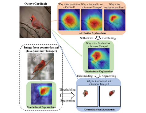
Figure 1: Given a query image (Cardinal) and a counterfactual class (Summer Tanager), discriminant explanations bridge the gap between attributions and counterfactual explanations. This enables a fast optimization-free computation of the latter.

Both problems can be addressed by explainable AI (XAI) techniques, which complement network predictions with human-understandable explanations. These can both circumvent the black-box nature of DL and enable the design of machine teaching systems that provide feedback to annotators when they make mistakes [43]. In computer vision, the dominant XAI paradigm is attribution, which consists of computing a heatmap of how strongly each image pixel [31, 3, 29, 1] or region [41, 28] contributes to a network prediction. For example, when asked “why is this a truck?” an attributive system would answer or visualize something like “because it has wheels, a hood, seats, a steering wheel, a flatbed, head and tail lights, and rearview mirrors.”

While useful to a naive user, this explanation is less useful to an expert in the domain. The latter is likely to be interested in more precise feedback, asking instead the question “Why is it not a car?” The answer “because it has a flatbed. If it did not have a flatbed it would be a car,” is known as a counterfactual or contrastive explanation [36, 8, 24]. Such explanations are more desirable in expert domains. When faced with a prediction of lesion $A$, a doctor would naturally ask “why $A$ but not $B$?” The same question would be posed by a student that incorrectly assigned an image to class $B$ upon receiving feedback that it belongs to class $A$. By supporting a specific query with respect to a counterfactual class ($B$), these explanations allow expert users to zero-in on a specific ambiguity between two classes, which they already know to be plausible prediction outcomes. Unlike attributions, counterfactual explanations scale naturally with user expertise. As the latter increases, the class and counterfactual class simply become more fine-grained.

In computer vision, counterfactual explanations have only recently received attention. They are usually implemented as “correct class is $A$. Class $B$ would require changing the image as follows,” where “as follows” is some visual transformations. Possible transformations include image perturbations [8], synthesis [36] or the exhaustive search of a large feature pool, to find replacement features that map the image from class $A$ to $B$ [12]. However, image perturbations and synthesis frequently leave the space of natural images only working on simple non-expert domains, and feature search is too complex for interactive applications.

In this work, a new procedure is proposed to generate Self-aware disCriminant cOUnterfactual explanaTions (SCOUT). We show that counterfactual explanations can be much more efficiently generated by a combination of attributive explanations and self-awareness mechanisms, which quantify the confidence of the predictions of a DL system. For this, we start by introducing discriminant explanations that, as shown in Figure 1, connect attributive to counterfactual explanations. Like attributive explanations, they consist of a single heatmap. This, however, is an attribution map for the discrimination of classes $A$ and $B$, attributing high scores to image regions that are informative of $A$ but not of $B$. In this sense, discriminant explanations are similar to counterfactual explanations and more precise than attributive explanations (see Figure 1). A counterfactual explanation can then be produced by the computation of two discriminant explanations, with the roles of $A$ and $B$ reversed.

We next consider how to compute discriminant explanations and argue for the importance of self-awareness. A system is self-aware if it can quantify the confidence with which it classifies an image. This is generally true for DL systems, which complement a class prediction with an estimate of the posterior class distribution, from which a confidence score can be derived [10, 39]. The attribution map of this score is an indicator of the image regions where the classification is easy. This fits nicely in the discriminant explanation framework, where the goal is to find the spatial regions predictive of class A but unpredictive of class B. It leads to the definition of discriminant explanations as image regions that simultaneously: 1) have high attribution for class $A$, 2) have low attribution for class $B$, and 3) are classified with high confidence. It follows that, as shown in Figure 1, discriminant explanations can be computed by combination of three attribution maps. This, in turn, shows that counterfactual explanations can be seen as a generalization of attributive explanations and computed by a combination of attribution [31, 3, 29, 34, 1] and confidence prediction methods [10, 39, 37] that is much more efficient to compute than previous methods.

Beyond explanations, a significant challenge to XAI is the lack of explanation ground truth for performance evaluation. Besides user-based evaluations [12], whose results are difficult to replicate, we propose a quantitative metric based on a proxy localization task. To the best of our knowledge, this is the first proposal for semantically quantitative evaluation of counterfactual visual explanations independently of human experiments. Compared to the latter, the proposed proxy evaluation is substantially easier to replicate. This evaluation shows that SCOUT both outperforms the state of the art [12] and is $50\times$ to $1000\times$ faster for popular networks. This is quite important for applications such as machine teaching, where explanation algorithms should operate in real-time, and ideally in low-complexity platforms such as mobile devices.

Overall, the paper makes five contributions. First, a new family of discriminant explanations, which are substantially more precise than attributive explanations. Second, the use of self-awareness to improve the accuracy of attributive explanations. Third, the derivation of counterfactual explanations by combination of discriminant explanations, making them more efficient to compute. Fourth, a new experimental protocol for quantitative evaluation of counterfactual explanations. Fifth, experimental results using both this protocol and machine teaching experiments, showing that the proposed SCOUT outperforms previous methods and is substantially faster.

2 Related work

In this section we review the literature on explanations, self-awareness, and machine teaching.

Explanations: Two main approaches to explainable AI (XAI) have emerged in computer vision. Natural language (NL) systems attempt to produce a textual explanation understandable to humans [13, 2, 26]. Since image to text translation is still a difficult problem, full blown NL explanations tend to target specific applications, like self driving [6]. More robust systems tend to use a limited vocabulary, e.g. a set of image attributes [2, 13]. For example, [2] proposed counterfactual NL image descriptions and [13] produces counterfactual explanations by extracting noun phrases from the counter-class, which are filtered with an evidence checker. Since phrases are defined by attributes, this boils down to detecting presence/absence of attributes in the query image. These methods require a priori definition of a vocabulary (e.g. attributes), training data for each vocabulary term, and training of the classifier to produce this side information. Due to these difficulties, most explanation methods rely instead on visualizations. While the ideas proposed in this work could be extended to NL systems, we consider only visual explanations.

Attributive explanations: The most popular approach to visual explanations is to rely on attributions [3, 29, 34]. These methods produce a heatmap that encodes how much the classifier prediction can be attributed to each pixel or image region. Many attribution functions have been proposed [31, 3, 29, 34, 1]. The most popular framework is to compute some variant of the gradient of the classifier prediction with respect a chosen layer of the network and then backproject to the input [28, 41]. These techniques tend to work well when the object of the predicted class is immersed in a large background (as in object detection), but are less useful when the image contains the object alone (as in recognition). In this setting, the most suitable for the close inspection required in expert domains, the heat map frequently covers the whole object. This is illustrated in Figure 1. Counterfactual explanations, which involve differences with respect to a counterfactual class, tend not to suffer from this problem.

Counterfactual explanations: Given an image of class $A$ and a counterfactual class $B$, counterfactual explanations (also known as contrastive [8]) produce an image transformation that elicits the classification as $B$ [35, 36, 21, 44]. The simplest example are adversarial attacks [8, 35, 43], which optimize perturbations to map an image of class $A$ into class $B$. However, adversarial perturbations usually push the perturbed image outside the boundaries of the space of natural images. Generative methods have been proposed to address this problem, computing large perturbations that generate realistic images [21, 23]. This is guaranteed by the introduction of regularization constraints, auto-encoders, or GANs [11]. However, because realistic images are difficult to synthesize, these approaches have only been applied to simple MNIST or CelebA [22] style datasets, not expert domains. A more plausible alternative is to exhaustively search the space of features extracted from a large collection of images, to find replacement features that map the image from class $A$ to $B$ [12]. While this has been shown to perform well on fine-grained datasets, exhaustive search is too complex for interactive applications.

Evaluation: The performance of explanation algorithms is frequently only illustrated by the display of visualizations. In some cases, explanations are evaluated quantitatively with recourse to human experiments. This involves the design of a system to elicit user feedback on how trustful a deep learning system is [28, 12, 8, 38] or evaluate if explanations improve user performance on some tasks [12]. While we present results of this type, they have several limitations: it can be difficult to replicate system design, conclusions can be affected by the users that participate in the experiments, and the experiments can be cumbersome to both set up and perform. In result, the experimental results are rarely replicable or even comparable. This hampers the scalable evaluation of algorithms. In this work, we introduce a quantitative protocol for the evaluation of counterfactual explanations, which overcomes these problems.

Self-awareness: Self-aware systems are systems with some abilities to measure their limitations or predict failures. This includes topics such as out-of-distribution detection [14, 20, 7, 18, 19] or open set recognition [27, 5], where classifiers are trained to reject non-sensical images, adversarial attacks, or images from classes on which they were not trained. All these problems require the classifier to produce a confidence score for image rejection. The most popular solution is to guarantee that the posterior class distribution is uniform, or has high entropy, outside the space covered by training images [18, 15]. This, however, is not sufficient for counterfactual explanations, which require more precise confidence scores explicitly addressing class $A$ or $B$. In this sense, the latter are more closely related to realistic classification [37], where a classifier must identify and reject examples that it deems too difficult to classify.

Machine teaching: Machine teaching systems [43] are usually designed to teach some tasks to human learners, e.g. image labeling. These systems usually leverage a model of student learning to optimize teaching performance [33, 4, 17, 25]. Counterfactual explanations are naturally suited for machine teaching, because they provide feedback on why a mistake (the choice of the counterfactual class $B$) was made. While the goal of this work is not to design a full blown machine teaching system, we investigate if counterfactual explanations can improve human labeling performance. This follows the protocol introduced by [12], which highlights matching bounding boxes on paired images (what part of $A$ should be replaced by what part of $B$) to provide feedback to students. Besides improved labeling performance, the proposed explanations are orders of magnitude faster than the exhaustive search of [12].

3 Discriminant Counterfactual Explanations

In this section, we briefly review the main ideas behind previous explanation approaches and introduce the proposed explanation technique.

Counterfactual explanations: Consider a recognition problem, mapping images $\mathbf{x}\in\mathcal{X}$ into classes $y\in\mathcal{Y}=\{1,\ldots,C\}$. Images are classified by an object recognition system $\mathcal{H}:\mathcal{X}\rightarrow\mathcal{Y}$ of the form

$$y^{*}=\arg\max_{y}h_{y}({\bf x}),$$ (1)

where ${\bf h}({\bf x}):{\cal X}\rightarrow[0,1]^{C}$ is a C-dimensional probability distribution with $\sum_{y=1}^{C}h_{y}({\bf x})=1$, usually computed by a convolutional neural network (CNN). The classifier is learned on a training set $\mathcal{D}$ of $N$ i.i.d. samples $\mathcal{D}=\{(\mathbf{x}_{i},y_{i})\}^{N}_{i=1}$, where $y_{i}\in\mathcal{Y}$ is the label of image $\mathbf{x}_{i}\in\mathcal{X}$, and its performance evaluated on a test set $\mathcal{T}=\{(\mathbf{x}_{j},y_{j})\}^{M}_{j=1}$. Given an image $\mathbf{x}$, for which the classifier predicts class $y^{*}$, counterfactual explanations answer the question of why the image does not belong to a counterfactual class (also denoted counter class) $y^{c}\neq y^{*}$, chosen by the user who receives the explanation.

Visual explanations: Counterfactual explanations for vision systems are usually based on visualizations. Two possibilities exist. The first is to explicitly transform the image $\mathbf{x}$ into an image $\mathbf{x}^{c}$ of class $y^{c}$, by replacing some of its pixel values. The transformation can consist of applying an image perturbation akin to those used in adversarial attacks [8], or replacing regions of $\mathbf{x}$ by regions of some images in the counter class $y^{c}$ [12]. Due to the difficulties of realistic image synthesis, these methods are only feasible when $\mathbf{x}$ is relatively simple, e.g. an MNIST digit.

A more plausible alternative is to use an already available image $\mathbf{x}^{c}$ from class $y^{c}$ and highlight the differences between $\mathbf{x}$ and $\mathbf{x}^{c}$. [12] proposed to do this by displaying matched bounding boxes on the two images, and showed that explanation performance is nearly independent of the choice of $\mathbf{x}^{c}$, i.e. it suffices to use a random image $\mathbf{x}^{c}$ from class $y^{c}$. We adopt a similar strategy in this work. For these approaches, the explanation consists of

$${\cal C}(\mathbf{x},y^{*},y^{c},\mathbf{x}^{c})=(\mathbf{c}^{*}(\mathbf{x}),\mathbf{c}^{c}(\mathbf{x}^{c})),$$ (2)

where $\mathbf{c}^{*}(\mathbf{x})$ and $\mathbf{c}^{c}(\mathbf{x}^{c})$ are counterfactual heatmaps for images $\mathbf{x}$ and $\mathbf{x}^{c}$, respectively, from which region segments $\mathbf{r}^{*}(\mathbf{x})$ and $\mathbf{r}^{c}(\mathbf{x}^{c})$ can be obtained, usually by thresholding. The question is how to compute these heatmaps. [12] proposed to search by exhaustively matching all combinations of features in $\mathbf{x}$ and $\mathbf{x}^{c}$, which is expensive. In this work, we propose a much simpler and more effective procedure that leverages a large literature on attributive explanations.

Attributive explanations: Attributive explanations are a family of explanations based on the attribution of the prediction $y^{*}$ to regions of $\mathbf{x}$ [31, 3, 29, 34, 1]. They are usually produced by applying an attribution function to a tensor of activations ${\bf F}\in\mathbb{R}^{W\times H\times D}$ of spatial dimensions $W\times H$ and $D$ channels, extracted at any layer of a deep network. While many attribution functions have been proposed, they are usually some variant of the gradient of $h_{y^{*}}(\mathbf{x})$ with respect to ${\bf F}$. This results in an attribution map $a_{i,j}(\mathbf{x})$ whose amplitude encodes the attribution of the prediction to each entry $i,j$ along the spatial dimensions of ${\bf F}$. Attributive explanations produce heat maps of the form

$$\mathcal{A}(\mathbf{x},y^{*})=\mathbf{a}(h_{y^{*}}(\mathbf{x}))$$ (3)

for some attribution function $\mathbf{a}(.)$. Two examples of attributive heatmaps of an image of a ”Cardinal,” with respect to predictions ”Cardinal” and ”Summer Tanager,” are shown in the top row of Figure 1.

Discriminant explanations: In this work, we propose a new class of explanations, which is denoted as discriminant and defined as

$${\cal D}(\mathbf{x},y^{*},y^{c})=\mathbf{d}(h_{y^{*}}(\mathbf{x}),h_{y^{c}}(\mathbf{x})),$$ (4)

which have commonalities with both attributive and counterfactual explanations. Like counterfactual explanations, they consider both the prediction $y^{*}$ and a counterfactual class $y^{c}$. Like attributive explanations, they compute a single attribution map through $\mathbf{d}(.,.)$. The difference is that this map attributes the discrimination between the prediction $y^{*}$ and counter $y^{c}$ class to regions of $\mathbf{x}$. While $\mathbf{a}(h_{y^{*}}(\mathbf{x}))$ assigns large attribution to pixels that are strongly informative of class $y^{*}$, $\mathbf{d}(h_{y^{*}}(\mathbf{x}),h_{y^{c}}(\mathbf{x}))$ does the same to pixels that are strongly informative of class $y^{*}$ but uninformative of class $y^{c}$.

Discriminant explanations can be used to compute counterfactual explanations by implementing (2) with

$${\cal C}(\mathbf{x},y^{*},y^{c},\mathbf{x}^{c})=({\cal D}(\mathbf{x},y^{*},y^{c}),{\cal D}(\mathbf{x}^{c},y^{c},y^{*})).$$ (5)

The first map identifies the regions of $\mathbf{x}$ that are informative of the predicted class but not the counter class while the second identifies the regions of $\mathbf{x}^{c}$ informative of the counter class but not of the predicted class. Altogether, the explanation shows that the regions highlighted in the two images are matched: the region of the first image depicts features that only appear in the predicted class while that of the second depicts features that only appear in the counterfactual class. Figure 1 illustrates the construction of a counterfactual explanation with two discriminant explanations.

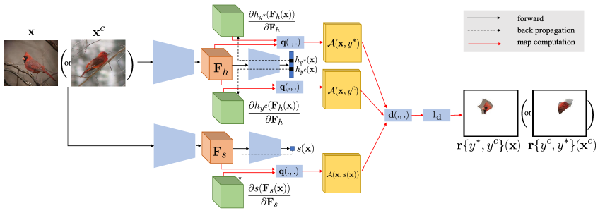
Figure 2: Discriminant explanation architecture ($\mathbf{x}$: Cardinal, $\mathbf{x}^{c}$: Summer Tanager.). Feature activations $\mathbf{F}_{h}$ and $\mathbf{F}_{s}$ are computed for some layers of the classifier (upper branch) and confidence predictor (lower branch), respectively. Attributions for prediction $h_{y^{*}}$, counter class $h_{y^{c}}$, and confidence score $s$ are computed by attribution functions $q(.,.)$ according to (10) and then combined with (6) to obtain the discriminant map. Counterfactual explanations are obtained by reversing the roles of $\mathbf{x}$ and $\mathbf{x}^{c}$ and thresholding the discriminant heat maps.

Self-awareness: Discriminant maps could be computed by combining attributive explanations with respect to the predicted and counter class. Assuming that binary ground truth segmentation maps $s^{*}_{i,j}$ and $s^{c}_{i,j}$ are available for the attributions of the predicted and counter classes, respectively, this could be done with the segmentation map $s_{i,j}=s^{*}_{i,j}.(1-s^{c}_{i,j}).$ This map would identify image regions attributable to the predicted class $y^{*}$ but not the counter class $y^{c}$. In practice, segmentation maps are not available and can only be estimated from attribution maps $a^{*}_{i,j}$ and $a^{c}_{i,j}$. While this could work well when the two classes are very different, it is not likely to work when they are similar. This is because, as shown in Figure 1, attribution maps usually cover substantial parts of the object. When the two classes differ only in small parts or details, they lack the precision to allow the identification of the associated regions. This is critical for expert domains, where users are likely to ask questions involving very similar classes.

Addressing this problem requires some ways to sharpen attribution maps. In this work, we advocate for the use of self-awareness. We assume that the classifier produces a confidence score $s({\bf x})\in[0,1]$, which encodes the strength of its belief that the image belongs to the predicted class. Regions that clearly belong to the predicted class $y^{*}$ render a score close to $1$ while regions that clearly do not render a score close to $0$. This score is self-referential if generated by the classifier itself and not self-referential if generated by a separate network. The discriminant maps of (4) are then implemented as

$$\mathbf{d}(h_{y^{*}}(\mathbf{x}),h_{y^{c}}(\mathbf{x}))=\mathbf{a}(h_{y^{*}}(\mathbf{x}))\cdot\overline{\mathbf{a}}(h_{y^{c}}(\mathbf{x}))\cdot\mathbf{a}(s(\mathbf{x}))$$ (6)

where $\overline{\mathbf{a}}(.)$ is the complement of $\mathbf{a}(.)$, i.e.

$$\overline{\mathbf{a}}_{i,j}=\max_{i,j}\mathbf{a}_{i,j}-\mathbf{a}_{i,j}.$$ (7)

The discriminant map $\mathbf{d}$ is large only at locations $(i,j)$ that contribute strongly to the prediction of class $y^{*}$ but little to that of class $y^{c}$, and where the discrimination between the two classes is easy, i.e. the classifier is confident. This, in turn, implies that location $(i,j)$ is strongly specific to class $y^{*}$ but non specific to class $y^{c}$, which is the essence of the counterfactual explanation. Figure 1 shows how the self-awareness attribution map is usually much sharper than the other two maps.

Segmentations: For discriminant explanations, the discriminant map of $\mathbf{x}$ is thresholded to obtain the segmentation mask

$$\mathbf{r}\{y^{*},y^{c}\}({\mathbf{x}})=\mathbbm{1}_{\mathbf{d}(h_{y^{*}}(\mathbf{x}),h_{y^{c}}(\mathbf{x}))>T},$$ (8)

where $\mathbbm{1}_{\cal S}$ is the indicator function of set $\cal S$ and $T$ a threshold. For counterfactual explanations, segmentation masks are also generated for $\mathbf{x}^{c}$, using

$$\mathbf{r}\{y^{c},y^{*}\}({\mathbf{x}}^{c})=\mathbbm{1}_{\mathbf{d}(h_{y^{c}}(\mathbf{x}^{c}),h_{y^{*}}(\mathbf{x}^{c}))>T}.$$ (9)

Attribution maps: The attribution maps of (6) can be computed with any attribution function $\mathbf{a}(.)$ in the literature [34, 29, 3]. In our implementation, we use the gradient-based function of [30]. This calculates the dot-product of the partial derivatives of the prediction $p$ with respect to the activations $\mathbf{F}(\mathbf{x})$ of a CNN layer and the activations, i.e.

$$a_{i,j}(h_{p})=q\left({\bf f}_{i,j},\frac{\partial h_{p}({\bf F})}{\partial{\bf f}_{i,j}}\right)=\left\langle\frac{\partial h_{p}({\bf F})}{\partial{\bf f}_{i,j}},{\bf f}_{i,j}\right\rangle,$$ (10)

where we omit the dependency on $\mathbf{x}$ for simplicity.

Confidence scores: Like attribution maps, many existing confidence or hardness scores can be leveraged. We considered three scores of different characteristics. The softmax score [10] is the largest class posterior probability

$$s^{s}({\bf x})=\max_{y}h_{y}({\bf x}).$$ (11)

It is computed by adding a max pooling layer to the network output. The certainty score is the complement of the normalized entropy of the softmax distribution [39],

$$s^{c}({\bf x})=1+\frac{1}{\log C}\sum_{y}h_{y}({\bf x})\log h_{y}({\bf x}).$$ (12)

Its computation requires an additional layer of $\log$ non-linearities and average pooling. These two scores are self-referential. We also consider the non-self-referential easiness score of [37],

$$s^{e}({\bf x})=1-s^{hp}({\bf x})$$ (13)

where $s^{hp}({\bf x})$ is computed by an external hardness predictor $\mathcal{S}$, which is jointly trained with the classifier. $\mathcal{S}$ is implemented with a network $s^{hp}({\bf x}):{\cal X}\rightarrow[0,1]$ whose output is a sigmoid unit.

Network implementation: Figure 2 shows a network implementation of (6). Given a query image $\mathbf{x}$ of class $y^{*}$, a user-chosen counter class $y^{c}\neq y^{*}$, a predictor $h_{y}(\mathbf{x})$, and a confidence predictor $s(\mathbf{x})$ are used to produce the explanation. Note that $s(\mathbf{x})$ can share weights with $h_{y}(\mathbf{x})$ (self-referential) or be separate (non-self-referential). $\mathbf{x}$ is forwarded through the network, generating activation tensors $\mathbf{F}_{h}(\mathbf{x})$, $\mathbf{F}_{s}(\mathbf{x})$ in pre-chosen network layers and predictions $h_{y^{*}}(\mathbf{x})$, $h_{y^{c}}(\mathbf{x})$, $s(\mathbf{x})$. The attributions of $y^{*}$, $y^{c}$ and $s(\mathbf{x})$ to $\mathbf{x}$, i.e. $\mathcal{A}(\mathbf{x},y^{*})$, $\mathcal{A}(\mathbf{x},y^{c})$, $\mathcal{A}(\mathbf{x},s(\mathbf{x}))$ are then computed with (10), which reduce to a backpropagation step with respect to the desired layer activations and a few additional operations. Finally, the three attributions are combined with (6). Thresholding the resulting heatmap with (8) produces the discriminant explanation $\mathbf{r}\{y^{*},y^{c}\}({\mathbf{x}})$. To further obtain a counterfactual explanation, the network is simply applied to $\mathbf{x}^{c}$ and $\mathbf{r}\{y^{c},y^{*}\}({\mathbf{x}}^{c})$ computed.

4 Evaluation

Challenges: Explanations are difficult to evaluate because ground truth is unavailable. Previous works mainly presented qualitative results [13, 12]. [12] also performed a human evaluation on MTurk, using a machine teaching task. However, this evaluation had a few flaws, which are discussed in Section 5.4. In any case, human evaluation is cumbersome and difficult to replicate. To avoid this, we introduce an alternative evaluation strategy based on the proxy task of localization. Because this leverages datasets with annotations for part locations and attributes, we sometimes refer to image regions (segments or keypoints) as parts.

Ground-truth: The goal of counterfactual explanations is to localize a region predictive of class $A$ but unpredictive of class $B$. Hence, parts with attributes specific to $A$ and that do not appear in $B$ can be seen as ground truth counterfactual regions. This enables the evaluation of counterfactual explanations as a part localization problem. To synthesize ground truth, the $k^{th}$ part of an object of class $c$ is represented by a semantic descriptor $\phi^{k}_{c}$ containing the attributes present in this class. For example, an “eye” part can have color attributes “red”, “blue”, “grey”, etc. The descriptor is a probability distribution over these attributes, characterizing the attribute variability of the part under each class.

The dissimilarity between classes $a$ and $b$, according to part $k$, is defined as $\alpha^{k}_{a,b}=\gamma(\phi^{k}_{a},\phi^{k}_{b})$, where $\gamma(.,.)$ is a dataset dependent function. Large dissimilarities indicate that part $k$ is a discriminant for classes $a$ and $b$. The values of $\alpha^{k}_{a,b}$ are computed for all class pairs $(a,b)$ and parts $\mathbf{p}_{k}$. The $M$ triplets $\mathcal{G}=\{(\mathbf{p}_{i},a_{i},b_{i})\}^{M}_{i=1}$ of largest dissimilarity are selected as counterfactual ground-truth.

Evaluation metrics: The metrics of explanation performance depend on the nature of part annotations. On datasets where part locations are labelled with a single point, i.e. $\mathbf{p}_{i}$ is a point (usually the geometric center of the part), the quality of region $\mathbf{r}\{a,b\}(\mathbf{x})$ is calculated by precision (P) and recall (R), where $P=\frac{J}{|\{k|\mathbf{p}_{k}\in\mathbf{r}\}|}$, $R=\frac{J}{|\{i|(\mathbf{p}_{i},a_{i},b_{i})\in\mathcal{G},a_{i}=a,b_{i}=b\}|}$, and $J=|\{i|\mathbf{p}_{i}\in\mathbf{r},a_{i}=a,b_{i}=b\}|$ is the number of included ground truth parts of generated regions. Precision-recall curves are produced by varying the threshold $T$ used in (8). For datasets where parts are annotated with segmentation masks, the quality of $\mathbf{r}\{a,b\}({\bf x})$ is evaluated using the intersection over union (IoU) metric $\text{IoU}=\frac{|\mathbf{r}\cap\mathbf{p}|}{|\mathbf{r}\cup\mathbf{p}|}$, where $\mathbf{p}=\{\mathbf{p}_{i}|(\mathbf{p}_{i},a_{i},b_{i})\in\mathcal{G},a_{i}=a,b_{i}=b\}$.

For counterfactual explanations, we define a measure of the semantic consistency of two segments, $\mathbf{r}\{a,b\}(\mathbf{x})$ and $\mathbf{r}\{b,a\}(\mathbf{x}^{c})$, by calculating the consistency of the parts included in them. This is denoted as the part IoU (PIoU),

$$\text{PIoU}={\scriptstyle\frac{|\{k|(\mathbf{p}_{k},a,b)\in\mathbf{r}\{a,b\}({\bf x})\}\cap\{k|(\mathbf{p}_{k},b,a)\in\mathbf{r}\{b,a\}({\bf x}^{c})\}|}{|\{k|(\mathbf{p}_{k},a,b)\in\mathbf{r}\{a,b\}({\bf x})\}\cup\{k|(\mathbf{p}_{k},b,a)\in\mathbf{r}\{b,a\}({\bf x}^{c})\}|}}.$$ (14)

These metrics allow the quantitative comparison of different counterfactual explanation methods. On datasets with point-based ground truth, this is based on precision and recall of the generated counterfactual regions. On datasets with mask-based ground truth, the IoU is used. After conducting the whole process on both $\mathbf{x}$ and $\mathbf{x}^{c}$, PIoU can be computed to further measure the semantic matching between the highlighted regions in the two images. As long as the compared counterfactual regions of different methods have the same size, the comparison is fair. For SCOUT, region size can be controlled by manipulating $T$ in (8) and (9) .

User expertise has an impact on counterfactual explanations. Beginner users tend to choose random counterfactual classes, while experts tend to pick counterfactual classes similar to the true class. Hence, explanation performance should be measured over the two user types. In this paper, users are simulated by choosing a random counterfactual class $b$ for beginners and the class predicted by a small CNN for advanced users. Class $a$ is the prediction of the classifier used to generate the explanation, which is a larger CNN.

5 Experiments

All experiments are performed on two datasets. CUB200 [40] consists of $200$ fine-grained bird classes, annotated with $15$ part locations (points) including back, beak, belly, breast, crown, forehead, left/right eye, left/right leg, left/right wing, nape, tail and throat. Each part is associated with attribute information [40] and dissimilarities $\alpha^{k}_{a,b}$ are computed with $\gamma(\phi^{k}_{a},\phi^{k}_{b})=e^{\{\text{KL}(\bm{\phi}^{k}_{a}||\bm{\phi}^{k}_{b})+\text{KL}(\bm{\phi}^{k}_{b}||\bm{\phi}^{k}_{a})\}}$ [9], where $\phi^{k}_{c}$ is a probability distribution over all attributes of the $k^{th}$ part under class $c$ and KL is the Kullback-Leibler divergence. $M$ is chosen to leave $80\%$ largest triplets $({\bf p}_{i},a_{i},b_{i})$ as ground truth. The majority of $({\bf p}_{i},a_{i},b_{i})$ are selected because dissimilar parts dominate in $\alpha^{k}_{a,b}$ space.

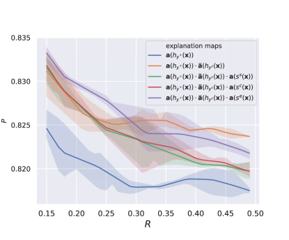
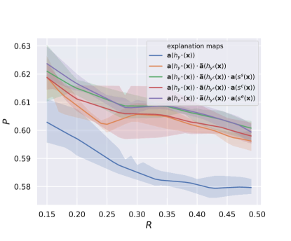
Figure 3: Comparison to attributive explanations. Left: beginners, right: advanced users.

The second dataset is ADE20K [42] with more than $1000$ fine-grained scene categories. Segmentation masks are given for $150$ objects. In this case, objects are seen as scene parts and each object has a single attribute, i.e. $\phi^{k}_{c}$ is scalar (where $k\in\{1,...,150\}$), which is the probability of occurrence of the object in a scene of class $c$. This is estimated by the relative frequency with which the part appears in scenes of class $c$. Ground truth consists of the triplets $({\bf p}_{i},a_{i},b_{i})$ with $\phi^{k}_{a}>0$ and $\phi^{k}_{b}=0$, i.e. where object $k$ appears in class $a$ but not in class $b$.

In the discussion below, results are obtained on CUB200, except as otherwise stated. ADE20K results are presented in the supplementary materials. Unless otherwise noted, visualizations are based on the last convolutional layer output of VGG16 [32], a widely used network in visualization papers. All counterfactual explanation results are presented for two types of virtual users. Randomly chosen labels mimic beginners while AlexNet predictions [16] mimic advanced users.

5.1 Comparison to attributive explanations

Figure 3 compares the discriminant explanations of (6), to attributive explanations $\mathbf{a}(h_{y^{*}}(\mathbf{x}))$, for the two user types. Several conclusions are possible: 1) discriminant maps significantly outperform attributions for both user types, independently of the confidence score used; 2) best performance is achieved with the easiness score of (13); 3) the gains are larger for expert users than beginners. This is because the counter and predicted classes tend to be more similar for the former and the corresponding attribution maps overlap. In this case, pure attributive explanations are very uninformative. The result also shows that self-awareness is most useful in expert domains.

5.2 Comparison to state of the art

		Beginner User		Advanced User
Arch.	Metric	Goyal [12]	SCOUT	Goyal [12]	SCOUT
VGG16	R	0.02 (0.01)	0.05 (0.01)	0.05 (0.00)	0.05 (0.00)
	P	0.76 (0.01)	0.84 (0.01)	0.56 (0.01)	0.64 (0.01)
	PIoU	0.13 (0.00)	0.15 (0.00)	0.09 (0.00)	0.14 (0.02)
	IPS	0.02 (0.00)	26.51 (0.71)
ResNet-50	R	0.03 (0.01)	0.09 (0.02)	0.12 (0.01)	0.16 (0.00)
	P	0.77 (0.01)	0.81 (0.01)	0.57 (0.02)	0.60 (0.01)
	PIoU	0.18 (0.01)	0.16 (0.01)	0.15 (0.00)	0.15 (0.01)
	IPS	1.13 (0.07)	78.54 (11.87)

Table 1: Comparison to the state of the art. (IPS: images per second, implemented on NVIDIA TITAN Xp. Results are shown as mean(stddev))

Table 1 presents a comparison between SCOUT and the method of [12] which obtained the best results by exhaustive search, for the two user types. For fair comparison, these experiments use the softmax score of (11), so that model sizes are equal for both approaches. The size of the counterfactual region is the receptive field size of one unit ($\frac{1}{14*14}\approx 0.005$ of image size on VGG16 and $\frac{1}{7*7}\approx 0.02$ on ResNet-50). This was constrained by the speed of the algorithm of [12], where the counterfactual region is detected by exhaustive feature matching.

Several conclusions could be drawn from the table. First, SCOUT outperforms [12] in almost all cases. Second, SCOUT is much faster, improving the speed of [12] by $1000+$ times on VGG and $50+$ times on ResNet. This is because it does not require exhaustive feature matching. These gains increase with the size of the counterfactual region, since computation time is constant for the proposed approach but exponential on region size for [12]. Third, due to the small size used in these experiments, PIoU is relatively low for both methods. It is, however, larger for the proposed explanations with large gains in some cases (VGG $\&$ advanced). Figure 4 shows that the PIoU can raise up to $0.5$ for regions of $10\%$ image size (VGG) or $20\%$ (ResNet). This suggests that, for regions of this size, the region pairs have matching semantics.

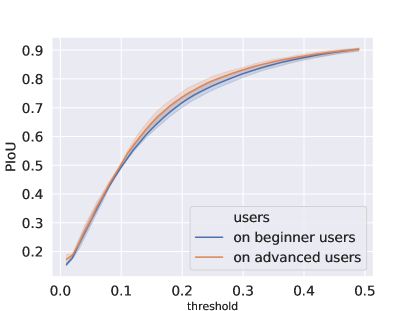
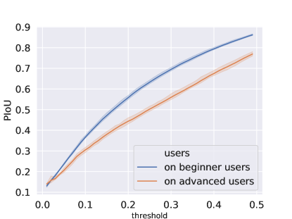
Figure 4: PIoU of SCOUT as a function of the segmentation threshold on CUB200. Left: VGG16, right: ResNet-50.

5.3 Visualizations

Figure 5 shows two examples of counterfactual visualizations derived from the ResNet50 on CUB200. The regions selected in the query and counter class image are shown in red. The true $y^{*}$ and counter $y^{c}$ class are shown below the images and followed by the ground truth discriminative attributes for the image pair. Note how the proposed explanations identify semantically matched and class-specific bird parts on both images. For example, the throat and bill that distinguish Laysan from Sooty Albatrosses. This feedback enables a user to learn that Laysans have white throats and yellow bills, while Sootys have black throats and bills. This is unlike the regions produced by [12], which sometimes highlight irrelevant cues, such as the background. Figure 6 presents similar figures for ADE20K, where the proposed explanations tend to identify scene-discriminative objects. For example, that a promenade deck contains objects ‘floor’, ‘ceiling’, ‘sea,’ while a bridge scene includes ‘tree’, ‘river’ and ‘bridge’.

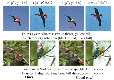
Figure 5: Comparison of counterfactual explanations (true and counter classes shown below each example, and ground truth class-specific part attributes in parenthesis).

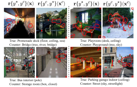
Figure 6: Counterfactual explanations on ADE20K.

5.4 Application to machine teaching

[12] used counterfactual explanations to design an experiment to teach humans distinguish two bird classes. During a training stage, learners are asked to classify birds. When they make a mistake, they are shown counterfactual feedback of the type of Figure 5, using the true class as $y^{*}$ and the class they chose as $y^{c}$. This helps them understand why they chose the wrong label, and learn how to better distinguish the classes. In a test stage, learners are then asked to classify a bird without visual aids. Experiments reported in [12] show that this is much more effective than simply telling them whether their answer is correct/incorrect, or other simple training strategies. We made two modifications to this set-up. The first was to replace bounding boxes with highlighting of the counterfactual reasons, as shown in Figure 7. We also instructed learners not to be distracted by the darkened regions. Unlike the set-up of [12], this guarantees that they do not exploit cues outside the counterfactual regions to learn bird differences. Second, to check this, we added two contrast experiments where 1) highlighted regions are generated randomly (without telling the learners); 2) the entire images are lighted. If these produce the same results, one can conclude that the explanations do not promote learning.

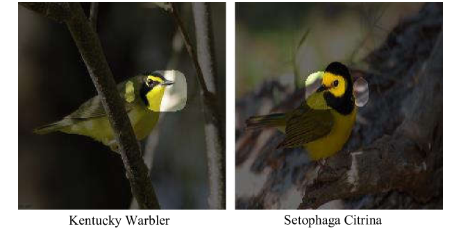
Figure 7: Visualization of machine teaching experiment.

We also chose two more difficult birds, the Setophaga Citrina and the Kentucky Warbler (see Figure 7), than those used in [12]. This is because these classes have large intra-class diversity. The two classes also cannot be distinguished by color alone, unlike those used in [12]. The experiment has three steps. The first is a pre-learning test, where students are asked to classify $20$ examples of the two classes, or choose a ‘Don’t know’ option. The second is a learning stage, where counterfactual explanations are provided for $10$ bird pairs. The third is a post-learning test, where students are asked to answer $20$ binary classification questions. In this experiment, all students chose ‘Don’t know’ in the pre-learning test. However, after the learning step, they achieved $95\%$ mean accuracy, compared to $60\%$ (random highlighted regions) and $77\%$ (entire images lighted) in the contrast settings. These results suggest that SCOUT can help teach non-expert humans distinguish categories from an expert domain.

6 Conclusion

In this work, we proposed a new family of discriminant explanations, which leverage self-awareness and bridge the gap between attributions and counterfactuals. A quantitative evaluation protocol was also proposed. Experiments under both this protocol and machine teaching experiments show that both the proposed discriminant and counterfactual explanations achieve much better performance than existing attributive and counterfactual methods.

Acknowledgements

This work was partially funded by NSF awards IIS-1637941, IIS-1924937, and NVIDIA GPU donations.

References

- [1] Marco Ancona, Enea Ceolini, Cengiz Öztireli, and Markus Gross. A unified view of gradient-based attribution methods for deep neural networks. In NIPS 2017-Workshop on Interpreting, Explaining and Visualizing Deep Learning. ETH Zurich, 2017.
- [2] Lisa Anne Hendricks, Ronghang Hu, Trevor Darrell, and Zeynep Akata. Grounding visual explanations. In The European Conference on Computer Vision (ECCV), September 2018.
- [3] Sebastian Bach, Alexander Binder, Grégoire Montavon, Frederick Klauschen, Klaus-Robert Müller, and Wojciech Samek. On pixel-wise explanations for non-linear classifier decisions by layer-wise relevance propagation. PloS one, 10(7):e0130140, 2015.
- [4] Sumit Basu and Janara Christensen. Teaching classification boundaries to humans. In Twenty-Seventh AAAI Conference on Artificial Intelligence, 2013.
- [5] Abhijit Bendale and Terrance E Boult. Towards open set deep networks. In Proceedings of the IEEE conference on computer vision and pattern recognition, pages 1563–1572, 2016.
- [6] Thierry Deruyttere, Simon Vandenhende, Dusan Grujicic, Luc Van Gool, and Marie-Francine Moens. Talk2car: Taking control of your self-driving car. arXiv preprint arXiv:1909.10838, 2019.
- [7] Terrance DeVries and Graham W Taylor. Learning confidence for out-of-distribution detection in neural networks. arXiv preprint arXiv:1802.04865, 2018.
- [8] Amit Dhurandhar, Pin-Yu Chen, Ronny Luss, Chun-Chen Tu, Paishun Ting, Karthikeyan Shanmugam, and Payel Das. Explanations based on the missing: Towards contrastive explanations with pertinent negatives. In Advances in Neural Information Processing Systems, pages 592–603, 2018.
- [9] Dominik Maria Endres and Johannes E Schindelin. A new metric for probability distributions. IEEE Transactions on Information theory, 2003.
- [10] Yonatan Geifman and Ran El-Yaniv. Selective classification for deep neural networks. In Advances in neural information processing systems, pages 4878–4887, 2017.
- [11] Ian Goodfellow, Jean Pouget-Abadie, Mehdi Mirza, Bing Xu, David Warde-Farley, Sherjil Ozair, Aaron Courville, and Yoshua Bengio. Generative adversarial nets. In Advances in neural information processing systems, pages 2672–2680, 2014.
- [12] Yash Goyal, Ziyan Wu, Jan Ernst, Dhruv Batra, Devi Parikh, and Stefan Lee. Counterfactual visual explanations. In Kamalika Chaudhuri and Ruslan Salakhutdinov, editors, Proceedings of the 36th International Conference on Machine Learning, volume 97 of Proceedings of Machine Learning Research, pages 2376–2384, 2019.
- [13] Lisa Anne Hendricks, Ronghang Hu, Trevor Darrell, and Zeynep Akata. Generating counterfactual explanations with natural language. arXiv preprint arXiv:1806.09809, 2018.
- [14] Dan Hendrycks and Kevin Gimpel. A baseline for detecting misclassified and out-of-distribution examples in neural networks. Proceedings of International Conference on Learning Representations, 2017.
- [15] Dan Hendrycks, Mantas Mazeika, and Thomas G Dietterich. Deep anomaly detection with outlier exposure. Proceedings of International Conference on Learning Representations, 2019.
- [16] Alex Krizhevsky and Geoffrey Hinton. Learning multiple layers of features from tiny images. Technical report, Citeseer, 2009.
- [17] Ronan Le Hy, Anthony Arrigoni, Pierre Bessière, and Olivier Lebeltel. Teaching bayesian behaviours to video game characters. Robotics and Autonomous Systems, 47(2-3):177–185, 2004.
- [18] Kimin Lee, Honglak Lee, Kibok Lee, and Jinwoo Shin. Training confidence-calibrated classifiers for detecting out-of-distribution samples. Proceedings of International Conference on Learning Representations, 2018.
- [19] Yi Li and Nuno Vasconcelos. Background data resampling for outlier-aware classification. In Proceedings of the IEEE Conference on Computer Vision and Pattern Recognition, 2020.
- [20] Shiyu Liang, Yixuan Li, and R Srikant. Enhancing the reliability of out-of-distribution image detection in neural networks. Proceedings of International Conference on Learning Representations, 2018.
- [21] Shusen Liu, Bhavya Kailkhura, Donald Loveland, and Yong Han. Generative counterfactual introspection for explainable deep learning. arXiv preprint arXiv:1907.03077, 2019.
- [22] Ziwei Liu, Ping Luo, Xiaogang Wang, and Xiaoou Tang. Deep learning face attributes in the wild. In Proceedings of International Conference on Computer Vision (ICCV), December 2015.
- [23] Ronny Luss, Pin-Yu Chen, Amit Dhurandhar, Prasanna Sattigeri, Karthikeyan Shanmugam, and Chun-Chen Tu. Generating contrastive explanations with monotonic attribute functions. arXiv preprint arXiv:1905.12698, 2019.
- [24] Tim Miller. Contrastive explanation: A structural-model approach. arXiv preprint arXiv:1811.03163, 2018.
- [25] Chris Piech, Jonathan Bassen, Jonathan Huang, Surya Ganguli, Mehran Sahami, Leonidas J Guibas, and Jascha Sohl-Dickstein. Deep knowledge tracing. In Advances in neural information processing systems, pages 505–513, 2015.
- [26] Shubham Rathi. Generating counterfactual and contrastive explanations using shap. arXiv preprint arXiv:1906.09293, 2019.
- [27] Walter J Scheirer, Anderson de Rezende Rocha, Archana Sapkota, and Terrance E Boult. Toward open set recognition. IEEE transactions on pattern analysis and machine intelligence, 35(7):1757–1772, 2012.
- [28] Ramprasaath R Selvaraju, Michael Cogswell, Abhishek Das, Ramakrishna Vedantam, Devi Parikh, and Dhruv Batra. Grad-cam: Visual explanations from deep networks via gradient-based localization. In Proceedings of the IEEE International Conference on Computer Vision, pages 618–626, 2017.
- [29] Avanti Shrikumar, Peyton Greenside, and Anshul Kundaje. Learning important features through propagating activation differences. In Proceedings of the 34th International Conference on Machine Learning-Volume 70, pages 3145–3153. JMLR. org, 2017.
- [30] Avanti Shrikumar, Peyton Greenside, Anna Shcherbina, and Anshul Kundaje. Not just a black box: Learning important features through propagating activation differences. arXiv preprint arXiv:1605.01713, 2016.
- [31] Karen Simonyan, Andrea Vedaldi, and Andrew Zisserman. Deep inside convolutional networks: Visualising image classification models and saliency maps. Workshop at International Conference on Learning Representations, 2014.
- [32] Karen Simonyan and Andrew Zisserman. Very deep convolutional networks for large-scale image recognition. arXiv preprint arXiv:1409.1556, 2014.
- [33] Adish Singla, Ilija Bogunovic, Gábor Bartók, Amin Karbasi, and Andreas Krause. Near-optimally teaching the crowd to classify. In ICML, page 3, 2014.
- [34] Mukund Sundararajan, Ankur Taly, and Qiqi Yan. Axiomatic attribution for deep networks. In Proceedings of the 34th International Conference on Machine Learning-Volume 70, pages 3319–3328. JMLR. org, 2017.
- [35] Arnaud Van Looveren and Janis Klaise. Interpretable counterfactual explanations guided by prototypes. arXiv preprint arXiv:1907.02584, 2019.
- [36] Sandra Wachter, Brent Mittelstadt, and Chris Russell. Counterfactual explanations without opening the black box: Automated decisions and the gpdr. Harv. JL & Tech., 31:841, 2017.
- [37] Pei Wang and Nuno Vasconcelos. Towards realistic predictors. In The European Conference on Computer Vision, 2018.
- [38] Pei Wang and Nuno Vasconcelos. Deliberative explanations: visualizing network insecurities. In Advances in Neural Information Processing Systems 32, pages 1374–1385, 2019.
- [39] Xin Wang, Yujia Luo, Daniel Crankshaw, Alexey Tumanov, Fisher Yu, and Joseph E Gonzalez. Idk cascades: Fast deep learning by learning not to overthink. arXiv preprint arXiv:1706.00885, 2017.
- [40] P. Welinder, S. Branson, T. Mita, C. Wah, F. Schroff, S. Belongie, and P. Perona. Caltech-UCSD Birds 200. Technical Report CNS-TR-2010-001, California Institute of Technology, 2010.
- [41] Bolei Zhou, Aditya Khosla, Agata Lapedriza, Aude Oliva, and Antonio Torralba. Learning deep features for discriminative localization. In Proceedings of the IEEE conference on computer vision and pattern recognition, pages 2921–2929, 2016.
- [42] Bolei Zhou, Hang Zhao, Xavier Puig, Sanja Fidler, Adela Barriuso, and Antonio Torralba. Scene parsing through ade20k dataset. In Proceedings of the IEEE Conference on Computer Vision and Pattern Recognition, 2017.
- [43] Xiaojin Zhu, Adish Singla, Sandra Zilles, and Anna N. Rafferty. An overview of machine teaching. arXiv preprint arXiv:1801.05927, 2018.
- [44] Luisa M Zintgraf, Taco S Cohen, Tameem Adel, and Max Welling. Visualizing deep neural network decisions: Prediction difference analysis. ICLR, 2017.