HST/FGS Trigonometric Parallaxes of M-dwarf Eclipsing Binaries

Abstract

Hubble Space Telescope (HST) Fine Guidance Sensor (FGS) trigonometric parallax observations were obtained to directly determine distances to five nearby M-dwarf / M-dwarf eclipsing binary systems. These systems are intrinsically interesting as benchmark systems for establishing basic physical parameters for low-mass stars, such as luminosity $L$, and radius $R$. HST/FGS distances are also one of the few direct checks on Gaia trigonometric parallaxes, given the comparable sensitivity in both magnitude limit and determination of parallactic angles. A spectral energy distribution (SED) fit of each system’s blended flux output was carried out, allowing for estimation of the bolometric flux from the primary and secondary components of each system. From the stellar $M$, $L$, and $R$ values, the low-mass star relationships between $L$ and $M$, and $R$ and $M$, are compared against idealized expectations for such stars. An examination on the inclusion of these close M-dwarf/M-dwarf pairs in higher-order common proper motion (CPM) pairs is analysed; each of the 5 systems has indications of being part of a CPM system. Unexpected distances on interesting objects found within the grid of parallactic reference stars are also presented, including a nearby M dwarf and a white dwarf.

1 Introduction

We obtained Hubble Space Telescope (HST) Fine Guidance Sensor (FGS) trigonometric parallax observations to directly determine distances to five nearby M-dwarf / M-dwarf eclipsing binary systems. Empirical distances yield or place constraints on the luminosities of these systems and individual components and consequently on low-mass stellar models. Fundamental astrophysical parameters of low-mass ($M<1M_{\odot}$) stars are of particular importance given that the large majority of the stars in the Galaxy are low-mass objects (Turnbull & Tarter, 2003; López-Morales & Ribas, 2005; Henry et al., 2006; Henry, 2007). While the accuracy of theoretically determined astrophysical parameters of low-mass stars is continuously being improved, there is still considerable disagreement between models and observation for both single stars and components of binary systems (Torres & Ribas, 2002; Ribas, 2003; Berger et al., 2006; Torres et al., 2010; Boyajian et al., 2012; von Braun et al., 2014; Mann et al., 2015; von Braun & Boyajian, 2017). Studying these objects is therefore crucial to understanding their intrinsic stellar astrophysics, the extent of their habitable zones, and the physics of the increasing number exoplanets being discovered about these low mass stars (e.g., Dressing & Charbonneau, 2015; Ballard & Johnson, 2016; Ballard, 2019, and references therein).

Observationally, stellar luminosity is obtained from the combination of distance and bolometric flux. Eclipsing binaries are ideal candidates to reconcile those parameters predicted by models with the observational quantities. However, only a small number ($N\lesssim 10$) of nearby ($d<$150pc) eclipsing M-dwarf binaries are known (López-Morales, 2007), and their distance determinations are either poorly constrained or entirely unknown. Thus, even with known bolometric fluxes for these systems, their luminosities remain model dependent.

Between August 2005 and May 2009, HST was operating using only two of its originally six gyros. In 2007–2009, we observed the well-studied systems GU Boo, CM Dra, YY Gem, and the more recently discovered binaries NSVS01031772 (López-Morales et al., 2006, “NSVS0103” hereafter) and TrES-Her0-07621 (Creevey et al., 2005, “TrES-Her0” hereafter) using FGS (see Table 1). Both respective eclipsing components of each of these binary systems are M dwarfs. Two other nearby systems, NSVS07394765 (Coughlin & Shaw, 2007) and CU Cnc (Delfosse et al., 1999), unfortunately did not present enough observing opportunities in HST’s two-gyro mode for parallax determination with FGS.

Of these seven systems, only CU Cnc is found in the Hipparcos catalog, with a 5.67 mas parallax error (Perryman et al., 1997); YY Gem can be found in the Yale GCTP with a 2.5 mas parallax error (van Altena et al., 1995); the other five systems had no trigonometric parallaxes available, clearly illustrating the paucity of distance information for these systems at the time. This has more recently been addressed via a recent FGS study by Benedict et al. (2016) measuring trigonometric parallaxes of M-dwarf binaries, and, of course, the recent release of Gaia Data Release 2 (DR2; Gaia Collaboration et al., 2018) provides an interesting astrometric comparison data set relative to our HST/FGS results. These observations – selected for HST orbits long before Gaia flew – provide a compelling cross-check on Gaia results. While that mission has proven itself to be a superlative source of distances and other astrophysical data, it is not infallible - for example, the Gaia DR2 distance on benchmark star RR Lyr is spurious with a value of $\pi=-2.61\pm 1.15$.

In order to calculate stellar luminosities, we supplement our direct distances based on trigonometric parallaxes with empirical estimates of the bolometric fluxes of the binary systems, as well as the bolometric fluxes of the respective individual stellar components, based on spectral energy distribution (SED) fitting of spectral templates to broad-band and narrow-band photometry. An ancillary product of this approach is an estimate of the angular stellar diameter for every stellar component of every system, which provide a sanity check to their counterparts produced by the studies of the eclipsing binary systems. Finally, all of our targets have dynamically determined masses with errors less than $0.5$%, which, coupled with directly determined distances as model-independent constraints, provide important anchors for the low mass end of the mass-luminosity relationship.

We describe our observations in §2, which include the HST/FGS observations and the selection of astrometric reference stars with respect to which trigonometric parallaxes of targets are measured (§2.1), plus spectroscopy and photometry for our targets and astrometric reference stars (§2.2 and 2.3). §3 describes our data analysis, including SED fitting (§3.1), the determination of the bolometric flux values of the individual components of our target systems (§3.2), distance calculations to the reference stars (§3.3) and target stars (§3.4), and comparisons with $Gaia$ values (3.5). Serendipitous findings within our data can be found in §4, such as the direct distance determination to a white dwarf and another M-dwarf. The distance-enabled astrophysics is presented in §5. We conclude in §6.

2 Observations

Parallax observations can be subdivided into observations from global astrometry (i.e. Gaia), and small- or single-field astrometry (i.e. HST/FGS); for an expanded discussion comparing two approaches, see the discussion in §2 of Benedict et al. (2017) and references therein. The HST/FGS method of trigonometric parallax is based on measuring relative positions of foreground target stars with respect to background reference stars at different phase angles during the Earth’s motion around the Sun. In order to convert these data to absolute distances, we estimate the distances to the background stars by collecting ancillary photometric and spectroscopic data. With spectral types and luminosity classes determined from the spectra, we use photometry to construct spectral energy distributions to determine interstellar reddening, absolute magnitude, and hence distance, for each reference star. This allows us to correct the positions of the reference stars measured by the FGS for residual astrometric motion caused by their parallaxes; thereby converting the distances measured for the M-dwarf eclipsing binaries to an absolute value. These distance estimates and final astrometric model are computed and presented in §3.

2.1 HST/FGS Observations

The HST/FGS instrument is described in Nelan (2012), and an overview of results from the FGS is presented by Benedict et al. (2017). The astrometric data from this program are available through the HST Program Information website for program 11213.

The target and reference stars were observed following the methodology described in Benedict et al. (2007), incorporating seven epochs of observations on each object spread over 1.5 to 2.0 years (Table 1). During our observations, FGS-1r was in POS mode using the astrometrically calibrated F583W filter. Multiple observations were obtained of the target and the reference stars available in the field during each HST orbit. All targets except TrES-Her0 are brighter than $V=14$, requiring minimal (1.2 minute) exposure time and overhead per target. The exposure and overhead requirements for TrES-Her0 were still small ($<$5 minutes), compared to a nominal 53 minute window of observations during each orbit. Data sets were taken at epochs closest to maximum parallactic excursion, with sets at the available far ends of the Cycle calendar window (July 2007 - December 2009) in order to disentangle parallax and proper motion effects and exclude times of eclipse of the binary system. An example of expected parallactic excursion on the sky is plotted for CM Dra in Figure 1.

During the course of the observations, HST was restricted to two-gyro pointing mode. The impact of this restriction was that roll angles and times of observations for targets at particular sky locations were limited to certain values or not possible at all. As noted in Section 1, two otherwise appealing targets for this study (CU Cnc and NSVS07394765) were unavailable due to this mode. For the available targets, restrictions in roll angle limited our options for selection of parallactic background reference stars, which required judicious scheduling of FGS observations, as we illustrate in Figure 2. Because of the limitations on the roll angle, sometimes only a subset of the reference stars could be observed during a given epoch.

The FGS data were reduced and calibrated as described in McArthur et al. (2001), Benedict et al. (2002a, b, 2007), and Soderblom et al. (2005); a more recent investigation using FGS is presented in some detail in Chaboyer et al. (2017). In general, the FGS reduction pipeline extracts the position of each star observed in the field and applies corrections for geometric distortion, differential velocity aberrations, spacecraft jitter, and drift. These positions are used as input to the astrometric model discussed in Section 3.4.

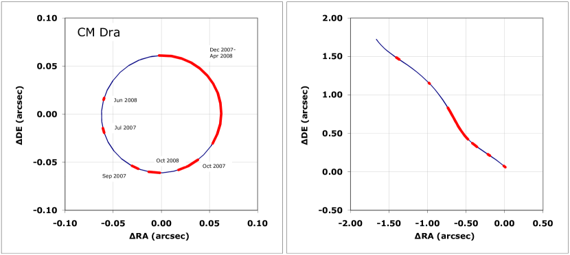
Figure 1: Right panel: Observed motion of the system on the sky, which includes the effects of parallax and proper motion. Left panel: Parallactic ellipse expected for the CM Dra system, isolated from proper motion effects. In both panels, the HST/FGS epochs of observation are indicated by the red points. For more details, see §2.1.

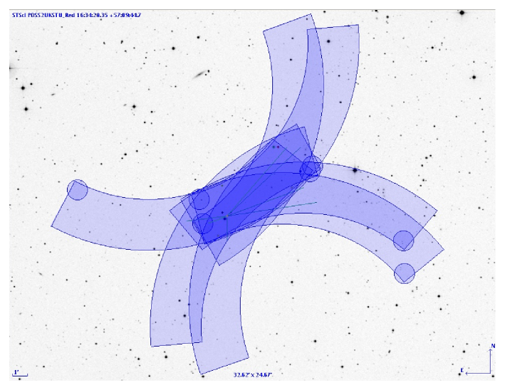
Figure 2: ‘Pickle plots’ of the HST/FGS field-of-view (FOV). Top: Multiple epochs of on-sky projections of the HST/FGS FOV for CM Dra. Bottom: The reference epoch for the astrometric fit for the CM Dra field showing the residuals in the positions of target and reference stars over the course of the FGS observations. For more details, see §2.1.

Table 1: FGS Observing Log.

Target	UT Date	UT Time
CM DRA	2007-09-07	01:12
	2008-01-02	05:30
	2008-02-24	04:24
	2008-06-15	19:15
	2008-07-07	07:13
	2008-12-17	03:13
	2009-09-20	03:24
GU Boo	2007-12-08	01:03
	2008-01-12	00:13
	2008-03-26	20:44
	2008-05-22	16:11
	2008-07-04	13:36
	2008-12-06	03:24
	2008-12-21	18:57
NSVS0103	2007-10-29	01:23
	2008-01-15	01:58
	2008-05-03	15:19
	2008-06-12	08:40
	2008-08-06	00:51
	2008-09-21	01:37
	2008-12-20	02:59
TRES-HER0	2007-10-21	03:37
	2008-01-02	00:04
	2008-03-23	14:30
	2008-07-01	12:11
	2008-09-25	12:58
	2009-01-02	20:11
YY GEM	2007-11-01	22:00
	2007-12-15	19:26
	2008-02-05	16:41
	2008-09-15	12:49
	2008-09-15	20:49
	2008-11-02	13:15
	2008-12-13	16:54

Note. — For more details, see §2.1.

2.2 WIYN HYDRA Spectra

To classify the spectral types and luminosity classes of the reference stars, we used the Hydra multi-fiber spectrograph on the WIYN 3.5 m telescope at Kitt Peak. We used the blue fiber cable with the BG-39 filter and a grating of 600 lines mm^-1 blazed at 13.9^∘ in the second order. This setup provided spectra from 3800 to 5200 Å  at a dispersion of 0.70 Å pixel^-1 with a resolving power of 1,581. This spectral region has numerous lines that are useful for determining spectral types and luminosity classifications (e.g. Gray’s Digital Classification Atlas). We recorded the data using the Bench Spectrograph Camera.

The Hydra spectra were obtained on UT 2010 April 23-26. We acquired spectra on all of the reference stars using one to two fiber positioning setups per FGS field. Total integration times per star ranged from 10 to 40 minutes. In each field we assigned 13$-$19 sky fibers for removing the background sky. We also obtained dome flats in the blue circle fiber configuration and bias frames. For wavelength calibration, we acquired CuAr lamp spectra for each fiber configuration. The spectra were flat-fielded, extracted, wavelength calibrated, and sky subtracted using the IRAF Hydra package.

We flattened the spectra using a spectral rectification technique that removes the shape of the stellar continuum, interstellar reddening, atmospheric extinction, and instrument response (LaSala & Kurtz, 1985). In this procedure, we took the Fourier transform of every spectrum, padded the ends by applying a cosine bell apodization, and put it through a low-pass filter to remove the high frequency Fourier components. We then transformed this spectrum back to get the underlying shape of the continuum and divided it out from the original spectrum to flatten it. Spectral classification was performed by comparing relative line strengths of the reference stars with spectral standards observed with the same instrument by H. E. Bond (e.g., Bond et al., 2013). The spectral templates included A, F, G, K, and M-type stars of main sequence, sub-giant, and giant classes with known spectral types. We also observed a few more spectral standard stars during our run with Hydra to cover a broader range of spectral sub-types. The spectral types and luminosity classes determined for the FGS reference stars are listed in Table 2. Plots of the spectra are shown in Figures 3–7.

Figure 3: Reference star spectra for CM Dra. For more information, see §2.2.

Figure 4: Reference star spectra for GU Boo. For more information, see §2.2.

Figure 5: Reference star spectra for NSVS0103. For more information, see §2.2.

Figure 6: Reference star spectra for TrES-Her0. For more information, see §2.2.

Figure 7: Reference star spectra for YY Gem. For more information, see §2.2.

Table 2: Target and reference star coordinates, photometry, and inferred spectral type: Johnson UBVRI and 2MASS JHKs.

Program ID	RA	DE	U	B	V	R	I	J	H	Ks	Spectral
	(hms)	(dms)	(mag)	(mag)	(mag)	(mag)	(mag)	(mag)	(mag)	(mag)	Type
CM-DRA	16 34 20.417	+57 09 43.93	…	$14.45\pm 0.01$	$12.92\pm 0.00$	$11.63\pm 0.01$	$9.99\pm 0.04$	$8.50\pm 0.02$	$8.04\pm 0.03$	$7.80\pm 0.02$	M4.5V
CM-DRA-REF45	16 33 57.786	+57 14 23.13	$15.55\pm 0.07$	$14.23\pm 0.01$	$13.41\pm 0.01$	…	…	$11.76\pm 0.02$	$11.32\pm 0.03$	$11.21\pm 0.02$	G8V?
CM-DRA-REF46	16 33 55.605	+57 14 23.16	$14.93\pm 0.07$	$14.93\pm 0.00$	$14.24\pm 0.01$	…	…	$13.08\pm 0.02$	$12.79\pm 0.03$	$12.75\pm 0.03$	G2V
CM-DRA-REF47	16 34 22.591	+57 09 59.81	$17.35\pm 0.07$	$15.50\pm 0.02$	$15.03\pm 0.02$	…	…	$14.11\pm 0.03$	$14.08\pm 0.04$	$14.14\pm 0.06$	wd
CM-DRA-REF58	16 33 44.447	+57 12 46.29	$15.36\pm 0.07$	$15.28\pm 0.02$	$14.58\pm 0.02$	…	…	$13.24\pm 0.02$	$12.82\pm 0.03$	$12.75\pm 0.03$	G5-G6V
CM-DRA-REF65	16 34 22.925	+57 11 46.70	$16.38\pm 0.07$	$16.17\pm 0.02$	$15.32\pm 0.01$	…	…	$13.76\pm 0.03$	$13.29\pm 0.03$	$13.33\pm 0.03$	K0V
CM-DRA-REF66	16 33 48.569	+57 11 40.86	$13.38\pm 0.07$	$13.46\pm 0.01$	$12.91\pm 0.01$	…	…	$11.83\pm 0.02$	$11.58\pm 0.03$	$11.53\pm 0.02$	F9V
CM-DRA-REF94	16 34 24.625	+57 08 26.94	$15.65\pm 0.07$	$15.33\pm 0.01$	$14.37\pm 0.01$	…	…	$12.59\pm 0.02$	$12.04\pm 0.02$	$11.94\pm 0.02$	K0III
GU-BOO	15 21 54.838	+33 56 09.25	…	$14.90\pm 0.02$	$13.65\pm 0.02$	$12.92\pm 0.11$	$12.09\pm 0.07$	$11.05\pm 0.02$	$10.36\pm 0.03$	$10.22\pm 0.02$	M0/M1.5V
GU-BOO-REF01	15 22 01.145	+34 01 05.89	$15.77\pm 0.07$	$15.56\pm 0.02$	$14.65\pm 0.02$	…	…	$12.98\pm 0.03$	$12.52\pm 0.04$	$12.44\pm 0.03$	K0V
GU-BOO-REF05	15 21 50.732	+34 00 32.70	$16.60\pm 0.07$	$16.35\pm 0.05$	$15.40\pm 0.02$	…	…	$13.75\pm 0.03$	$13.19\pm 0.04$	$13.13\pm 0.03$	K0-K2V
GU-BOO-REF08	15 22 05.555	+34 00 02.18	$14.14\pm 0.07$	$14.44\pm 0.03$	$13.85\pm 0.03$	…	…	$12.49\pm 0.02$	$12.13\pm 0.03$	$12.03\pm 0.02$	F9V
GU-BOO-REF25	15 21 58.531	+34 00 10.86	$17.01\pm 0.07$	$16.29\pm 0.03$	$15.27\pm 0.01$	…	…	$13.28\pm 0.02$	$12.70\pm 0.03$	$12.57\pm 0.02$	K3V
GU-BOO-REF51	15 22 20.585	+33 52 14.83	$15.02\pm 0.07$	$14.47\pm 0.05$	$13.31\pm 0.06$	…	…	$11.37\pm 0.02$	$10.87\pm 0.02$	$10.77\pm 0.02$	K3V
GU-BOO-REF53	15 21 56.870	+33 58 37.57	$14.99\pm 0.07$	$15.24\pm 0.03$	$14.67\pm 0.02$	…	…	$13.51\pm 0.02$	$13.15\pm 0.04$	$13.08\pm 0.03$	G0V
GU-BOO-REF57	15 21 57.397	+33 55 29.10	$15.83\pm 0.07$	$15.95\pm 0.03$	$15.32\pm 0.01$	…	…	$14.12\pm 0.03$	$13.79\pm 0.03$	$13.77\pm 0.04$	G2V
NSVS0103	13 45 34.953	+79 23 48.61	…	$15.06\pm 0.23$	$13.52\pm 0.09$	…	…	$9.69\pm 0.02$	$9.02\pm 0.02$	$8.78\pm 0.02$	M2-M3V
NSVS0103-REF00	13 44 02.121	+79 23 49.48	…	$14.54\pm 0.01$	$13.76\pm 0.01$	…	…	$12.39\pm 0.02$	$12.01\pm 0.02$	$11.96\pm 0.02$	G8V
NSVS0103-REF01	13 46 21.316	+79 21 34.95	…	$15.00\pm 0.02$	$14.30\pm 0.01$	…	…	$13.02\pm 0.02$	$12.69\pm 0.02$	$12.59\pm 0.03$	G5V
NSVS0103-REF02	13 47 30.350	+79 23 37.52	…	$11.47\pm 0.01$	$10.77\pm 0.01$	…	…	$9.50\pm 0.02$	$9.17\pm 0.02$	$9.05\pm 0.02$	G5V
NSVS0103-REF05	13 45 41.357	+79 21 05.38	…	$15.70\pm 0.02$	$14.78\pm 0.01$	…	…	$13.08\pm 0.02$	$12.61\pm 0.02$	$12.49\pm 0.02$	K2V
NSVS0103-REF19	13 46 37.263	+79 18 47.62	…	$14.37\pm 0.02$	$13.66\pm 0.01$	…	…	$12.29\pm 0.02$	$11.91\pm 0.02$	$11.79\pm 0.02$	G3V
NSVS0103-REF23	13 45 20.334	+79 18 01.73	…	$13.20\pm 0.01$	$12.62\pm 0.01$	…	…	$11.53\pm 0.02$	$11.25\pm 0.02$	$11.17\pm 0.02$	G0V
NSVS0103-REF68	13 45 55.139	+79 23 14.00	…	$17.30\pm 0.04$	$15.78\pm 0.02$	…	…	$11.64\pm 0.02$	$11.03\pm 0.02$	$10.76\pm 0.02$	M4.5V
NSVS0103-REF96	13 46 58.399	+79 22 04.23	…	$13.52\pm 0.02$	$13.02\pm 0.01$	…	…	$12.00\pm 0.02$	$11.76\pm 0.02$	$11.70\pm 0.02$	F6V
TRES-HER0	16 50 20.771	+46 39 01.61	…	$17.23\pm 0.05$	$15.76\pm 0.03$	$14.58\pm 0.02$	$13.14\pm 0.04$	$11.77\pm 0.02$	$11.14\pm 0.02$	$10.88\pm 0.02$	M2-M3 V
TRES-HER0-REF337	16 50 03.823	+46 43 17.02	…	$11.86\pm 0.00$	$11.39\pm 0.01$	…	…	$10.41\pm 0.02$	$10.17\pm 0.02$	$10.16\pm 0.02$	F5V
TRES-HER0-REF347	16 50 13.877	+46 41 26.68	$14.25\pm 0.07$	$14.48\pm 0.01$	$13.88\pm 0.01$	…	…	$12.64\pm 0.02$	$12.30\pm 0.02$	$12.26\pm 0.02$	G0V
TRES-HER0-REF363	16 50 58.817	+46 38 49.20	$15.68\pm 0.07$	$15.17\pm 0.01$	$14.22\pm 0.01$	…	…	$12.41\pm 0.02$	$11.87\pm 0.02$	$11.77\pm 0.02$	K3V
TRES-HER0-REF377	16 50 50.869	+46 36 46.17	$14.83\pm 0.07$	$14.43\pm 0.01$	$13.56\pm 0.01$	…	…	$12.03\pm 0.02$	$11.65\pm 0.02$	$11.55\pm 0.02$	K0V
TRES-HER0-REF380	16 50 48.218	+46 36 32.09	$14.48\pm 0.07$	$14.67\pm 0.01$	$14.12\pm 0.01$	…	…	$13.03\pm 0.02$	$12.77\pm 0.03$	$12.72\pm 0.03$	F8III
TRES-HER0-REF394	16 49 56.216	+46 33 36.03	$12.75\pm 0.07$	$12.01\pm 0.00$	$10.93\pm 0.01$	…	…	$9.02\pm 0.03$	$8.51\pm 0.02$	$8.39\pm 0.02$	K2IIIab
TRES-HER0-REF823	16 50 44.114	+46 37 11.08	$15.96\pm 0.07$	$16.20\pm 0.03$	$15.47\pm 0.01$	…	…	$13.94\pm 0.03$	$13.53\pm 0.03$	$13.44\pm 0.05$	G2V
YY-GEM	07 34 37.446	+31 52 10.22	…	…	…	…	…	$6.07\pm 0.02$	$5.42\pm 0.02$	$5.24\pm 0.02$	M1.0Ve
YY-GEM-REF01	07 34 52.068	+31 52 34.14	…	…	…	…	…	$9.34\pm 0.02$	$8.83\pm 0.03$	$8.69\pm 0.02$	K0IIIb
YY-GEM-REF02	07 34 49.027	+31 51 42.87	…	…	…	…	…	$11.86\pm 0.02$	$11.56\pm 0.02$	$11.49\pm 0.02$	G3V
YY-GEM-REF03	07 34 26.315	+31 51 00.12	…	…	…	…	…	$8.27\pm 0.02$	$7.80\pm 0.02$	$7.69\pm 0.02$	K0III
YY-GEM-REF04	07 34 31.213	+31 51 16.65	…	…	…	…	…	$13.22\pm 0.02$	$12.94\pm 0.03$	$12.89\pm 0.03$	G0V
YY-GEM-REF05	07 34 41.849	+31 51 37.15	…	…	…	…	…	$15.19\pm 0.05$	$14.98\pm 0.08$	$14.78\pm 0.10$	G0V
YY-GEM-REF06	07 34 42.028	+31 51 58.49	…	…	…	…	…	$14.42\pm 0.05$	$14.31\pm 0.04$	$14.37\pm 0.07$	G2V
YY-GEM-REF07	07 34 31.228	+31 52 29.27	…	…	…	…	…	$12.41\pm 0.05$	$12.05\pm 0.05$	$11.89\pm 0.02$	G8V

Note. — For entries with ‘…’, no data were taken; photometric data collection is described in §2.3. Spectral types determined using the methodology described in §2.2 using data from this table and Table 3.

2.3 42- and 31-inch Photometry

CCD Photometry in the standard Johnson UBVRI and narrowband ‘Hale-Bopp’ filter sets (Farnham et al., 2000) was obtained for all our target stars and their astrometric reference stars, excepting YY Gem (see next paragraph) using Lowell Observatory’s Hall 42-inch and 31-inch telescope located at Anderson Mesa. Standard stars from Landolt (1983) and Farnham were used for atmospheric extinction correction. Johnson B and V was collected for all the stars (Table 2), as well as the narrowband filters (Table 3).

Given the proximity of YY Gem to Castor (roughly 1 arcminute away, and 8 magnitudes brighter), the Kron photometer on the Hall 42-inch was used instead of the CCD cameras to obtain narrowband data for this target and its reference stars. The Kron photometer is a single-element aperture photometer with a thermoelectrically cooled EMI6256 photomultiplier. While slightly more time-consuming than CCD observing – only one object can be observed at a time – the nature of the instrument’s sampling aperture allowed observations of YY Gem and its FGS reference stars to be conducted in a way to minimize and also allow subtraction of the scattered light from Castor. CCD observations of these targets with the CCD cameras on the 42- and 31-inch telescopes were not possible due to scattering and saturation effects of of Castor on the imaging chip. Kron photometer observations were compared to Farnham standards and extinction corrected and are found in Table 3.

Table 3: Target and reference star coordinates, photometry, and inferred spectral type: Hale-Bopp narrowband ‘comet’ filters.

Program ID	Bc	C2	C3	CN	COp	Gc	NH	OH	Rc	UVc	Spectral
	(mag)	(mag)	(mag)	(mag)	(mag)	(mag)	(mag)	(mag)	(mag)	(mag)	Type
CM-DRA	…	…	…	…	…	…	…	…	…	…	M4.5V
CM-DRA-REF45	$14.46\pm 0.01$	$13.43\pm 0.01$	$16.40\pm 0.06$	…	$14.42\pm 0.03$	…	…	…	…	…	G8V?
CM-DRA-REF46	$14.67\pm 0.01$	$14.38\pm 0.01$	$15.19\pm 0.06$	…	$15.15\pm 0.03$	$14.21\pm 0.02$	…	…	$13.31\pm 0.02$	…	G2V
CM-DRA-REF47	$16.20\pm 0.01$	…	…	…	$17.80\pm 0.03$	$16.22\pm 0.02$	…	…	$14.56\pm 0.02$	…	wd
CM-DRA-REF58	$15.08\pm 0.01$	$14.65\pm 0.01$	$15.73\pm 0.06$	…	$15.56\pm 0.03$	$14.61\pm 0.02$	…	…	$13.71\pm 0.02$	…	G5-G6V
CM-DRA-REF65	…	$15.47\pm 0.01$	…	…	$16.34\pm 0.03$	$15.34\pm 0.02$	…	…	…	…	K0V
CM-DRA-REF66	$13.36\pm 0.01$	$12.91\pm 0.01$	$13.77\pm 0.06$	…	$13.57\pm 0.03$	$12.88\pm 0.02$	…	…	$12.13\pm 0.02$	…	F9V
CM-DRA-REF94	$15.13\pm 0.01$	$14.48\pm 0.01$	$15.71\pm 0.06$	…	$15.77\pm 0.03$	$14.36\pm 0.02$	…	…	$13.28\pm 0.02$	…	K0III
GU-BOO	…	…	…	…	…	…	…	…	…	…	M0/M1.5V
GU-BOO-REF01	…	…	$15.47\pm 0.06$	…	$15.41\pm 0.03$	…	…	…	…	…	K0V
GU-BOO-REF05	$15.93\pm 0.01$	$15.61\pm 0.01$	$16.33\pm 0.06$	…	$16.12\pm 0.03$	$15.42\pm 0.02$	…	…	$14.36\pm 0.02$	…	K0-K2V
GU-BOO-REF08	$14.31\pm 0.01$	$13.90\pm 0.01$	$14.74\pm 0.06$	…	$14.58\pm 0.03$	$13.83\pm 0.02$	…	…	$12.94\pm 0.02$	…	F9V
GU-BOO-REF25	$16.17\pm 0.01$	$15.62\pm 0.01$	…	…	$16.89\pm 0.03$	$15.20\pm 0.02$	…	…	…	…	K3V
GU-BOO-REF51	$14.17\pm 0.01$	$13.62\pm 0.01$	$15.06\pm 0.06$	…	$14.80\pm 0.03$	$13.36\pm 0.02$	…	…	$12.14\pm 0.02$	…	K3V
GU-BOO-REF53	$15.09\pm 0.01$	$14.70\pm 0.01$	$15.32\pm 0.06$	…	$15.38\pm 0.03$	$14.58\pm 0.02$	…	…	$13.86\pm 0.02$	…	G0V
GU-BOO-REF57	$15.58\pm 0.01$	$15.25\pm 0.01$	$16.74\pm 0.06$	…	$15.80\pm 0.03$	$15.20\pm 0.02$	…	…	$14.23\pm 0.02$	…	G2V
NSVS0103	$15.14\pm 0.34$	$13.89\pm 0.09$	$16.22\pm 0.85$	$16.47\pm 0.90$	…	$13.64\pm 0.12$	…	…	…	…	M2-M3V
NSVS0103-REF00	$14.33\pm 0.16$	$13.79\pm 0.08$	$15.35\pm 0.38$	$15.12\pm 0.24$	…	$13.54\pm 0.11$	…	…	…	…	G8V
NSVS0103-REF01	$15.00\pm 0.29$	$14.52\pm 0.15$	$15.12\pm 0.30$	$16.05\pm 0.59$	…	$14.27\pm 0.20$	…	…	…	…	G5V
NSVS0103-REF02	$11.29\pm 0.02$	$10.88\pm 0.02$	$11.85\pm 0.02$	$12.48\pm 0.03$	…	$10.75\pm 0.02$	$12.55\pm 0.06$	…	…	…	G5V
NSVS0103-REF05	$15.21\pm 0.35$	$14.85\pm 0.21$	…	…	…	…	…	…	…	…	K2V
NSVS0103-REF19	$14.50\pm 0.19$	$13.65\pm 0.07$	$14.86\pm 0.25$	$15.03\pm 0.24$	…	$13.70\pm 0.13$	$15.37\pm 0.64$	…	…	…	G3V
NSVS0103-REF23	$13.14\pm 0.06$	$12.67\pm 0.03$	$13.58\pm 0.08$	$13.91\pm 0.09$	…	$12.57\pm 0.05$	$14.09\pm 0.20$	…	…	…	G0V
NSVS0103-REF68	…	$15.47\pm 0.36$	…	…	…	…	…	…	…	…	M4.5V
NSVS0103-REF96	$13.32\pm 0.07$	$13.03\pm 0.04$	$13.79\pm 0.09$	$14.04\pm 0.11$	…	$12.98\pm 0.07$	…	…	…	…	F6V
TRES-HER0	…	…	…	…	…	…	…	…	…	…	M2-M3 V
TRES-HER0-REF337	…	…	…	…	…	…	…	…	…	…	F5V
TRES-HER0-REF347	$14.31\pm 0.01$	$13.92\pm 0.01$	$14.69\pm 0.06$	…	$14.54\pm 0.03$	$13.84\pm 0.02$	…	…	$13.04\pm 0.02$	…	G0V
TRES-HER0-REF363	$14.98\pm 0.01$	$14.59\pm 0.01$	$15.84\pm 0.06$	…	$15.61\pm 0.03$	$14.25\pm 0.02$	…	…	$13.12\pm 0.02$	…	K3V
TRES-HER0-REF377	$14.21\pm 0.01$	$13.74\pm 0.01$	$14.86\pm 0.06$	…	$14.70\pm 0.03$	$13.60\pm 0.02$	…	…	$12.61\pm 0.02$	…	K0V
TRES-HER0-REF380	$14.51\pm 0.01$	$14.13\pm 0.01$	$14.97\pm 0.06$	…	$14.76\pm 0.03$	$14.02\pm 0.02$	…	…	$13.33\pm 0.02$	…	F8III
TRES-HER0-REF394	$11.86\pm 0.01$	$11.12\pm 0.01$	$12.73\pm 0.06$	…	$12.31\pm 0.03$	$11.01\pm 0.02$	…	…	$9.87\pm 0.02$	…	K2IIIab
TRES-HER0-REF823	$15.98\pm 0.01$	$15.42\pm 0.01$	$16.28\pm 0.06$	…	$16.29\pm 0.03$	$15.43\pm 0.02$	…	…	$14.53\pm 0.02$	…	G2V
YY-GEM	$10.33\pm 0.02$	$9.65\pm 0.01$	$11.40\pm 0.02$	$12.08\pm 0.03$	…	$9.24\pm 0.02$	$12.62\pm 0.05$	$13.37\pm 0.23$	…	$12.38\pm 0.04$	M1.0Ve
YY-GEM-REF01	$12.16\pm 0.03$	$11.44\pm 0.02$	$12.97\pm 0.04$	$14.05\pm 0.07$	…	$11.27\pm 0.02$	$14.19\pm 0.11$	…	…	$14.30\pm 0.10$	K0IIIb
YY-GEM-REF02	$13.61\pm 0.07$	$13.07\pm 0.04$	$13.91\pm 0.08$	$15.16\pm 0.23$	…	$13.05\pm 0.07$	$14.89\pm 0.25$	$15.15\pm 0.82$	…	$14.80\pm 0.17$	G3V
YY-GEM-REF03	$10.77\pm 0.02$	$10.12\pm 0.01$	$11.49\pm 0.02$	$12.50\pm 0.03$	…	$10.03\pm 0.02$	$12.80\pm 0.05$	…	…	$12.49\pm 0.03$	K0III
YY-GEM-REF04	$14.42\pm 0.13$	…	$15.00\pm 0.21$	$14.83\pm 0.14$	…	$14.16\pm 0.15$	$15.51\pm 0.46$	…	…	$15.38\pm 0.28$	G0V
YY-GEM-REF05	…	…	…	…	…	…	…	…	…	…	G0V
YY-GEM-REF06	$15.16\pm 0.30$	$15.03\pm 0.23$	…	…	…	$15.38\pm 0.56$	…	$15.29\pm 1.07$	…	…	G2V
YY-GEM-REF07	$13.73\pm 0.08$	$13.03\pm 0.04$	$14.06\pm 0.10$	$14.19\pm 0.10$	…	$12.99\pm 0.06$	$14.60\pm 0.18$	…	…	$14.59\pm 0.14$	G8V

Note. — For entries with ‘…’, no data were taken; photometric data collection is described in §2.3. For details on the Hale-Bopp narrowband ‘comet’ filters, see Farnham et al. (2000).Spectral types determined using the methodology described in §2.2 using data from this table and Table 2.

Table 4: Estimated and measured parameters for reference stars.

Program ID	Ang. Size	$F_{\rm BOL}$ a	$A_{V}$	Sp. Type	$R$ b	$d_{\rm R}$	$M_{V}$	$BC$	$d_{\rm MV}$ c	$d_{\rm final}$	$\pi_{\rm final}$	$\pi_{Gaia}$
	(mas)		(mag)		$(R_{\odot})$	(pc)	(mag)	(mag)	(pc)	(pc)	(mas)	(mas)
CM-DRA-REF45	$0.0295\pm 0.0021$	$23.30\pm 0.84$	$0.75\pm 0.02$	G8V	0.93	$294\pm 36$	5.5	-0.4	$220\pm 44$	$264\pm 52$	$3.786\pm 0.746$	$0.590\pm 0.016$
CM-DRA-REF46	$0.0131\pm 0.0009$	$5.48\pm 0.10$	$0.00\pm 0.02$	G2V	1.25	$886\pm 108$	4.7	-0.2	$847\pm 169$	$874\pm 27$	$1.144\pm 0.036$	$1.946\pm 0.204$
CM-DRA-REF58	$0.0121\pm 0.0009$	$4.97\pm 0.12$	$0.18\pm 0.02$	G5V	0.99	$757\pm 93$	5.1	-0.2	$683\pm 137$	$734\pm 52$	$1.363\pm 0.096$	$1.203\pm 0.023$
CM-DRA-REF65	$0.0097\pm 0.0007$	$2.55\pm 0.06$	$0.12\pm 0.02$	K0V	0.79	$763\pm 93$	5.9	-0.3	$711\pm 142$	$747\pm 36$	$1.338\pm 0.065$	$1.352\pm 0.032$
CM-DRA-REF66	$0.0217\pm 0.0015$	$19.20\pm 0.35$	$0.04\pm 0.02$	F9V	1.43	$614\pm 75$	4.2	-0.2	$552\pm 110$	$594\pm 43$	$1.683\pm 0.123$	$1.034\pm 0.029$
CM-DRA-REF94	$0.0214\pm 0.0015$	$6.66\pm 0.12$	$0.07\pm 0.02$	K0III	13.60	$5905\pm 723$	0.7	-0.5	$5381\pm 1076$	$5742\pm 370$	$0.174\pm 0.011$	$0.170\pm 0.018$
GU-BOO-REF01	$0.0143\pm 0.0010$	$5.57\pm 0.16$	$0.29\pm 0.02$	K0V	0.79	$516\pm 63$	5.9	-0.3	$444\pm 89$	$492\pm 51$	$2.032\pm 0.210$	$1.971\pm 0.240$
GU-BOO-REF05	$0.0101\pm 0.0007$	$2.77\pm 0.08$	$0.28\pm 0.02$	K0V	0.79	$731\pm 90$	5.9	-0.3	$635\pm 127$	$699\pm 68$	$1.430\pm 0.138$	$1.435\pm 0.026$
GU-BOO-REF08	$0.0169\pm 0.0012$	$11.70\pm 0.34$	$0.41\pm 0.02$	F9V	1.43	$788\pm 97$	4.2	-0.2	$596\pm 119$	$712\pm 136$	$1.405\pm 0.268$	$2.403\pm 0.041$
GU-BOO-REF25	$0.0154\pm 0.0011$	$3.79\pm 0.09$	$0.27\pm 0.02$	K3V	0.78	$469\pm 58$	6.7	-0.5	$412\pm 82$	$451\pm 40$	$2.220\pm 0.197$	$1.744\pm 0.023$
GU-BOO-REF51	$0.0354\pm 0.0025$	$20.00\pm 0.35$	$0.12\pm 0.02$	K3V	0.78	$204\pm 25$	6.7	-0.5	$192\pm 38$	$201\pm 9$	$4.988\pm 0.212$	$5.119\pm 0.022$
GU-BOO-REF53	$0.0106\pm 0.0008$	$4.18\pm 0.09$	$0.12\pm 0.02$	G0V	1.28	$1122\pm 137$	4.4	-0.2	$1046\pm 209$	$1099\pm 54$	$0.910\pm 0.044$	$1.065\pm 0.020$
GU-BOO-REF57	$0.0084\pm 0.0006$	$2.26\pm 0.04$	$0.00\pm 0.02$	G2V	1.25	$1376\pm 168$	4.7	-0.2	$1319\pm 264$	$1360\pm 41$	$0.736\pm 0.022$	$0.685\pm 0.025$
NSVS0103-REF00	$0.0187\pm 0.0013$	$9.34\pm 0.17$	$0.02\pm 0.02$	G8V	0.93	$464\pm 57$	5.5	-0.4	$488\pm 98$	$470\pm 17$	$2.129\pm 0.078$	$2.048\pm 0.015$
NSVS0103-REF01	$0.0132\pm 0.0009$	$5.94\pm 0.12$	$0.12\pm 0.02$	G5V	0.99	$694\pm 85$	5.1	-0.2	$643\pm 129$	$678\pm 35$	$1.474\pm 0.077$	$1.386\pm 0.016$
NSVS0103-REF02	$0.0669\pm 0.0047$	$153.00\pm 2.68$	$0.12\pm 0.02$	G5V	0.99	$137\pm 17$	5.1	-0.2	$127\pm 25$	$134\pm 7$	$7.473\pm 0.395$	$6.798\pm 0.030$
NSVS0103-REF05	$0.0141\pm 0.0010$	$4.17\pm 0.08$	$0.00\pm 0.02$	K2V	0.71	$469\pm 57$	6.4	-0.4	$491\pm 98$	$474\pm 16$	$2.108\pm 0.071$	$2.260\pm 0.018$
NSVS0103-REF19	$0.0192\pm 0.0014$	$12.20\pm 0.26$	$0.24\pm 0.02$	G3V	1.14	$553\pm 68$	4.8	-0.2	$479\pm 96$	$528\pm 52$	$1.893\pm 0.186$	$0.831\pm 0.014$
NSVS0103-REF23	$0.0262\pm 0.0019$	$25.60\pm 0.45$	$0.07\pm 0.02$	G0V	1.28	$454\pm 56$	4.4	-0.2	$432\pm 86$	$447\pm 16$	$2.235\pm 0.079$	$1.780\pm 0.022$
NSVS0103-REF68	$0.0553\pm 0.0039$	$11.00\pm 0.17$	$0.00\pm 0.03$	M4V	0.19	$32\pm 4$	11.5	-2.5	$74\pm 15$	$35\pm 29$	$28.614\pm 23.947$	$16.572\pm 0.048$
NSVS0103-REF96	$0.0194\pm 0.0014$	$18.50\pm 0.34$	$0.13\pm 0.02$	F6V	1.70	$815\pm 100$	3.7	-0.1	$682\pm 136$	$769\pm 94$	$1.301\pm 0.159$	$0.876\pm 0.026$
TRES-HER0-REF337	$0.0398\pm 0.0028$	$82.00\pm 1.45$	$0.13\pm 0.01$	F5V	1.83	$428\pm 52$	3.5	-0.1	$348\pm 70$	$399\pm 56$	$2.507\pm 0.352$	$1.863\pm 0.027$
TRES-HER0-REF347	$0.0159\pm 0.0011$	$9.47\pm 0.20$	$0.22\pm 0.02$	G0V	1.28	$748\pm 92$	4.4	-0.2	$662\pm 132$	$720\pm 61$	$1.389\pm 0.118$	$0.761\pm 0.016$
TRES-HER0-REF363	$0.0219\pm 0.0015$	$7.67\pm 0.12$	$0.00\pm 0.02$	K3V	0.78	$330\pm 40$	6.7	-0.5	$328\pm 66$	$329\pm 2$	$3.037\pm 0.014$	$3.053\pm 0.023$
TRES-HER0-REF377	$0.0216\pm 0.0015$	$12.70\pm 0.23$	$0.14\pm 0.02$	K0V	0.79	$342\pm 42$	5.9	-0.3	$316\pm 63$	$334\pm 18$	$2.995\pm 0.166$	$2.550\pm 0.016$
TRES-HER0-REF380	$0.0125\pm 0.0009$	$6.26\pm 0.10$	$0.00\pm 0.02$	F8III	5.25	$3901\pm 477$	1.2	-0.3	$4120\pm 824$	$3956\pm 155$	$0.253\pm 0.010$	$0.859\pm 0.021$
TRES-HER0-REF394	$0.1200\pm 0.0084$	$173.00\pm 2.37$	$0.00\pm 0.01$	K2III	19.00	$1471\pm 180$	0.5	-0.6	$1260\pm 252$	$1400\pm 150$	$0.714\pm 0.076$	$0.890\pm 0.022$
TRES-HER0-REF823	$0.0090\pm 0.0006$	$2.54\pm 0.08$	$0.32\pm 0.02$	G2V	1.25	$1296\pm 159$	4.7	-0.2	$1073\pm 215$	$1217\pm 158$	$0.822\pm 0.107$	$0.190\pm 0.032$
YY-GEM-REF01	$0.0984\pm 0.0070$	$141.00\pm 2.96$	$0.32\pm 0.02$	K0III	13.60	$1284\pm 157$	0.7	-0.5	$1042\pm 208$	$1196\pm 171$	$0.836\pm 0.120$	$0.883\pm 0.040$
YY-GEM-REF02	$0.0223\pm 0.0016$	$16.30\pm 0.29$	$0.00\pm 0.03$	G3V	1.14	$476\pm 58$	4.8	-0.2	$463\pm 93$	$472\pm 9$	$2.119\pm 0.042$	$2.444\pm 0.036$
YY-GEM-REF03	$0.1540\pm 0.0109$	$346.00\pm 5.65$	$0.00\pm 0.02$	K0III	13.60	$821\pm 101$	0.7	-0.5	$772\pm 154$	$806\pm 34$	$1.240\pm 0.053$	$1.079\pm 0.044$
YY-GEM-REF04	$0.0120\pm 0.0009$	$5.36\pm 0.14$	$0.00\pm 0.08$	G0V	1.28	$991\pm 122$	4.4	-0.2	$974\pm 195$	$987\pm 12$	$1.014\pm 0.012$	$0.704\pm 0.032$
YY-GEM-REF05	$0.0048\pm 0.0005$	$0.87\pm 0.12$	$0.08\pm 0.57$	G0V	1.28	$2468\pm 345$	4.4	-0.2	$2334\pm 467$	$2421\pm 95$	$0.413\pm 0.016$	$0.816\pm 0.084$
YY-GEM-REF06	$0.0064\pm 0.0005$	$1.30\pm 0.08$	$0.00\pm 0.32$	G2V	1.25	$1816\pm 229$	4.7	-0.2	$1739\pm 348$	$1792\pm 54$	$0.558\pm 0.017$	$\ldots$
YY-GEM-REF07	$0.0200\pm 0.0014$	$10.60\pm 0.23$	$0.00\pm 0.06$	G8V	0.93	$433\pm 53$	5.5	-0.4	$462\pm 92$	$441\pm 20$	$2.270\pm 0.104$	$2.040\pm 0.031$

Note. — Distances estimated from two methodologies: bolometric-flux estimated angular size vs. linear size estimates ($d_{\rm R}$), and bolometric-corrected estimates of $M_{\rm V}$. For more information, see Sections 3.1 and 3.3.

3 Analysis

3.1 Spectral Energy Distribution

We performed SED fits for every target and calibrator star. These fits take photometry described in §2.3 as input values, and subsequently fit template spectra to them. The choice of template spectra from Pickles (1998) is determined by the WIYN Hydra spectra described in §2.2. Each template is adjusted to account for overall flux level, wavelength-dependent reddening, and expected angular size. Reddening corrections are based upon the empirical reddening determination described by Cardelli et al. (1989), which differs little from van de Hulst’s theoretical reddening curve number 15 (Johnson, 1968; Dyck et al., 1996). We thus obtain estimates for every single star for regarding its bolometric flux ($F_{BOL}$) and interstellar reddening ($A_{V}$) along the line of sight. Based on the effective temperature values that are given for each of the Pickles (1998) templates, we also calculate stellar angular size ($\theta$). The results of the fitting are given in Table 4.

3.2 Binary SED data from binarySED

An extension of the sedFit code discussed in §3.1, binarySED, was developed for fitting of pairs of SED curves that make up a binary’s observed, blended SED. Just as the sedFit code can search for the individual best fit template for a given input set of photometry, binarySED will search using pairs of templates. Input data for binarySED is also broad- to narrow-band photometry, as well as a priori primary-secondary flux ratio estimates at defined bandpasses. The best-fit spectral templates for the two components of each binary are presented in Table 5.

The wavelength-dependent flux ratio estimates for the binaries are given in Table 6. For GU Boo, there is a particularly rich data set from López-Morales & Ribas (2005), covering multiple narrow bands from 532 to 714 nm. Other stars, such as CM Dra and NSVS0103, only have estimates for the $V$-, $R$-, and $I$-bands.

Table 5: Binary SEDfit results from this study on the systems of interest, along with literature values: parallax/distance, and primary/secondary spectral types.

			Literature			binarySED
Target	$\pi$	$d$	Primary	Secondary	Reference	Primary	Secondary
	(mas)	(pc)	SpType	SpType		SpType	SpType
TrES-Her0	$6.06\pm 0.47$	$165.0\pm 12.8$	K9.5	K9.5	Creevey et al. (2005)	M3	M3.5
CM Dra	$68.48\pm 0.43$	$14.60\pm 0.09$	M5	M5.5	Metcalfe et al. (1996)	M4	M4
GU Boo	$3.19\pm 0.60$	$313.5\pm 59.0$	K7	K7	López-Morales & Ribas (2005)	K8.5	M0
NSVS0103	$15.29\pm 0.58$	$65.40\pm 2.48$	K8.5	K9.5	López-Morales et al. (2006)	M1.5	M3.5
YY Gem	$67.22\pm 0.42$	$14.88\pm 0.09$	K7	K7	Torres & Ribas (2002)	M0.5	M0.5

Note. — For more information, see §3.2.

Table 6: Primary-secondary photometry ratio data used as input to binarySED.

Target	Wavelength	Bandpass	Ratio	Reference
	(nm)	(nm)
GU Boo	532.5	10	$0.75\pm 0.1$	López-Morales & Ribas (2005) (Figure 3)
GU Boo	552.5	10	$0.83\pm 0.1$	López-Morales & Ribas (2005) (Figure 3)
GU Boo	562.5	10	$0.88\pm 0.125$	López-Morales & Ribas (2005) (Figure 3)
GU Boo	572.5	10	$0.77\pm 0.15$	López-Morales & Ribas (2005) (Figure 3)
GU Boo	584	10	$0.875\pm 0.15$	López-Morales & Ribas (2005) (Figure 3)
GU Boo	585	10	$0.79\pm 0.15$	López-Morales & Ribas (2005) (Figure 3)
GU Boo	593	10	$0.77\pm 0.12$	López-Morales & Ribas (2005) (Figure 3)
GU Boo	595	10	$0.77\pm 0.14$	López-Morales & Ribas (2005) (Figure 3)
GU Boo	606	10	$0.82\pm 0.2$	López-Morales & Ribas (2005) (Figure 3)
GU Boo	612	10	$0.8\pm 0.15$	López-Morales & Ribas (2005) (Figure 3)
GU Boo	620	10	$0.925\pm 0.1$	López-Morales & Ribas (2005) (Figure 3)
GU Boo	626	10	$0.97\pm 0.125$	López-Morales & Ribas (2005) (Figure 3)
GU Boo	647.5	10	$0.92\pm 0.125$	López-Morales & Ribas (2005) (Figure 3)
GU Boo	662	10	$0.87\pm 0.175$	López-Morales & Ribas (2005) (Figure 3)
GU Boo	671	10	$0.79\pm 0.175$	López-Morales & Ribas (2005) (Figure 3)
GU Boo	705	10	$0.86\pm 0.2$	López-Morales & Ribas (2005) (Figure 3)
GU Boo	714	10	$0.86\pm 0.19$	López-Morales & Ribas (2005) (Figure 3)
CM Dra	555	89	$0.871\pm 0.125$	Chabrier & Baraffe (1995) (Table 1)
CM Dra	693	210	$0.8721\pm 0.032$	Morales et al. (2009) (Table 5)
CM Dra	879	171	$0.8782\pm 0.033$	Morales et al. (2009) (Table 5)
NSVS0103	555	89	$0.95\pm 0.05$	López-Morales et al. (2006)
NSVS0103	693	210	$1\pm 0.05$	López-Morales et al. (2006)
NSVS0103	879	171	$1\pm 0.05$	López-Morales et al. (2006)
TRES-HER0	555	89	$0.912\pm 0.046$	Creevey et al. (2005) (Table 3)
TRES-HER0	693	210	$0.92\pm 0.06$	Creevey et al. (2005) (Table 3)
TRES-HER0	879	171	$0.944\pm 0.08$	Creevey et al. (2005) (Table 3)
TRES-HER0	1250	250	$1\pm 0.1$	Creevey et al. (2005) (Table 3)
TRES-HER0	1650	300	$1\pm 0.1$	Creevey et al. (2005) (Table 3)
TRES-HER0	2200	400	$1\pm 0.1$	Creevey et al. (2005) (Table 3)
YY GEM	555	89	$1\pm 0.01$	Torres & Ribas (2002) (Table 4), Butler et al. (2015)
YY GEM	693	210	$1\pm 0.01$	Torres & Ribas (2002) (Table 4), Butler et al. (2015)
YY GEM	879	171	$1\pm 0.01$	Torres & Ribas (2002) (Table 4), Butler et al. (2015)

Note. — For more information on how this ratio data was used in binary sedFits of individual systems, see §3.2.

The output from binarySED is, separately for both the primary and secondary star, similar to the sedFit output. This includes an estimate of interstellar extinction for the binary pair ($A_{\rm V}$), and for each component, a measurement of the bolometric flux ($F_{\rm BOL}$). Based upon the effective temperature defined for the template that fits best for each stellar component, the apparent angular size is estimated ($\theta_{\rm EST}$). These results are presented in Table 7.

Table 7: Primary and secondary fit parameters from binarySED.

			Primary		Secondary
Target	$\chi^{2}$	System $F_{\rm BOL}$	$F_{\rm BOL}$	$\theta$	$F_{\rm BOL}$	$\theta$
TrES-Her0	12.55	$(8.97\pm 0.10)\times 10^{-11}$	$(4.36\pm 0.07)\times 10^{-11}$	$0.031\pm 0.002$	$(4.61\pm 0.07)\times 10^{-11}$	$0.034\pm 0.002$
CM Dra	22.36	$(1.62\pm 0.02)\times 10^{-09}$	$(8.62\pm 0.12)\times 10^{-10}$	$0.155\pm 0.011$	$(7.54\pm 0.12)\times 10^{-10}$	$0.145\pm 0.010$
GU Boo	13.74	$(2.21\pm 0.01)\times 10^{-10}$	$(1.12\pm 0.01)\times 10^{-10}$	$0.038\pm 0.002$	$(1.09\pm 0.01)\times 10^{-10}$	$0.040\pm 0.002$
NSVS0103	2.59	$(6.36\pm 0.32)\times 10^{-10}$	$(3.57\pm 0.28)\times 10^{-10}$	$0.091\pm 0.007$	$(2.79\pm 0.14)\times 10^{-10}$	$0.085\pm 0.007$
YY Gem	16.81	$(1.88\pm 0.01)\times 10^{-08}$	$(1.06\pm 0.01)\times 10^{-08}$	$0.411\pm 0.029$	$(9.52\pm 0.05)\times 10^{-09}$	$0.390\pm 0.027$

Note. — Units of $F_{\rm BOL}$ are erg cm^-2 s^-1 and $\theta$ are mas; estimates from binarySED include overall system bolometric flux (left column), and primary/secondary star fluxes and angular sizes (middle and right columns, respectively). For more information, see §3.2.

3.3 Inferred Reference Star Distances

Following the SED fitting described in §3.1, distances to the parallactic reference stars were estimated in two ways and are presented in Table 4. These two ways we interpreted the sedFit data are as follows: First, we compared the estimated angular size to linear size expected from the spectral type and compute the distance ($d_{R}$), since $d\propto R/\theta$. Second, we compared the §3.1 estimate of bolometric flux to the intrinsic bolometric flux expected from spectral type with the usual relationship, $m_{\rm V}-M_{\rm V}=5\log d+A_{V}$. From the sedFit measured bolometric flux $F_{\rm BOL}$, the bolometric magnitude $m_{\rm BOL}$ can be computed with the standard zeropoint of $2.48\times 10^{-5}$ erg cm^-2 s^-1 for $m_{\rm BOL}=0$ (Cox, 2000). For a given spectral type, Cox (2000) can also be referenced for values of $M_{\rm V}$ and $BC$; with $BC$, the $m_{\rm BOL}$ can be converted to $m_{V}$. Thus, all the elements for a flux-based estimate of the distance ($d_{MV}$) are obtained.

In Table 4 we list the spectral type, stellar radius, distance estimate $d_{R}$, $M_{V}$, $BC$, and distance estimate $d_{MV}$. The last column in Table presents the final adopted distances determined from an average of the two methods. Figure 8 shows a comparison of these reference star distances with parallaxes from the Gaia DR2 catalog (Gaia Collaboration et al., 2018).

Figure 8: Comparison of the spectrophotometric distances of the reference stars with Gaia DR2 parallaxes. The outlier / most discrepant result is CM-Dra-REF45; the reasons for the discrepancy are not known. For more details, see Section 3.3.

3.4 Trigonometric Parallaxes of FGS Target Stars

An astrometric model was fit to the FGS positions measured in §2.1 using the least squares estimation program GaussFit (Jefferys et al., 1988) following the method described by Bond et al. (2013) and Benedict et al. (2017). The model consists of a four parameter plate solution for each FGS epoch that accounts for the translation, rotation, and scale differences in the field of view during each observation. It also includes a lateral color correction (Benedict et al., 1999; Nelan & Bond, 2013). The model accounts for the proper motion and parallax of each star in the field of view. An expanded six parameter plate solution, which accommodates the additional adjustment of the relative scales along the x and y axis independently, did not change and/or improve our solutions by statistically significant amounts.

As input to GaussFit, we computed parallaxes for the reference stars from the distance estimates listed in Table 4 and assumed an uncertainty of 20%, which was consistent with the general spread between the two estimation techniques. The initial proper motions for the reference stars were collected from several catalogs including UCAC4 (Zacharias et al., 2013), UCAC5 (Zacharias et al., 2017), URAT (Zacharias et al., 2015), and PPMXL (Roeser et al., 2010). The UCAC5 presents an improved astrometric solution by combining the existing UCAC data with the first Gaia data release (Gaia Collaboration et al., 2016). The high proper motion star CM-DRA-REF47 was not included in the UCAC4, UCAC5, and URAT catalogs, so we adopted the proper motion for that star from Lépine & Shara (2005). We fit the FGS astrometric data using each set of initial proper motions. The GaussFit code varies the input parallaxes and proper motions of the reference stars within their uncertainties to solve for the best astrometric grid. The output proper motions showed a strong dependence on the input values, representing an absolute shift between different catalogs, as was discussed by Bond et al. (2013). However, the parallaxes of the target stars computed from each set of input proper motions were consistent with each other within the uncertainties ($<$ 0.3 $\sigma$). In Table 8 we present the parallaxes of the target stars derived from using the initial proper motions from UCAC5.

The astrometric fit for the YY Gem field did not include REF05 and REF06 because these stars were fainter than expected and the FGS acquisition failed. The astrometric fit for the NSVS0103 field did not include REF33; this star was observed in only two out of seven epochs and one of these observations had a very large residual in the fit position. It was removed from the model so that the solution would converge for the remaining stars.

The FGS parallaxes have errors from the fitting routine in the range of $0.4-0.6$ mas. This level of performance is slightly worse than that of Benedict et al. (2007) and VandenBerg et al. (2014), who achieved parallaxes with errors on order $\pm 0.25$ mas. This is likely due to the limitations on the available HST roll angles and the selection of background reference stars as described in §2.1.

In addition to the five M-dwarf eclipsing binaries, we found that two of the reference stars (NSVS0103-REF68 and CM-DRA-REF47) are at similar distances and form a common proper motion pair with the affiliated target star. We solved for the parallax of both stars from the FGS data. For NSVS0103-REF68 we also kept the proper motion as a free parameter, but could not do the same for CM-DRA-REF47. With only two observation dates that included CM-DRA-REF47, it was necessary to keep the input proper motion as a constraint in the astrometric grid. These stars are discussed in more detail in Section 4.

Based on these trigonometric parallaxes, the derived parameters for our target systems (mass, luminosity, and linear radius for each component) are presented in Table 9, incorporating the $F_{\rm BOL}$ and $\theta$ binarySED fit parameters noted in Table 7.

Table 8: FGS Parallaxes

Star	FGS - UCAC5	FGS - Gaia	Gaia DR2
	$\pi$ (mas)	$\pi$ (mas)	$\pi$ (mas)
CM-DRA	68.62 $\pm$ 0.44	68.23 $\pm$ 0.38	67.34 $\pm$ 0.05
CM-DRA-REF47	66.15 $\pm$ 2.57	65.10 $\pm$ 1.40	67.32 $\pm$ 0.02
GU-BOO	3.18 $\pm$ 0.59	3.15 $\pm$ 0.56	6.15 $\pm$ 0.02
NSVS0103	15.13 $\pm$ 0.57	14.92 $\pm$ 0.53	16.48 $\pm$ 0.03
NSVS0103-REF68	14.98 $\pm$ 0.70	14.84 $\pm$ 0.66	16.57 $\pm$ 0.05
TRES-HER0	5.89 $\pm$ 0.57	5.58 $\pm$ 0.53	7.11 $\pm$ 0.04
YY-GEM	67.34 $\pm$ 0.43	67.22 $\pm$ 0.40	66.23 $\pm$ 0.05

Note. — The FGS astrometric fits in the column labeled “FGS - UCAC5” use the UCAC5 proper motions and the spectrophotometric distance estimates as inputs for the reference stars (Section 3.4). The FGS astrometric fits in the column labeled “FGS - Gaia” use the Gaia DR2 proper motions and parallaxes as inputs for the reference stars (Section 3.5). The last column lists the parallaxes directly from the Gaia DR2 catalog for comparison.

Table 9: Primary and secondary derived parameters.

	Primary			Secondary
Target	M	L	R	M	L	R
TrES-Her0	$0.493\pm 0.003$	$0.037\pm 0.006$	$0.552\pm 0.058$	$0.489\pm 0.003$	$0.039\pm 0.006$	$0.600\pm 0.063$
CM Dra	$0.231\pm 0.001$	$0.0057\pm 0.0001$	$0.244\pm 0.017$	$0.214\pm 0.001$	$0.0050\pm 0.0001$	$0.228\pm 0.016$
GU Boo	$0.610\pm 0.007$	$0.345\pm 0.130$	$1.289\pm 0.248$	$0.599\pm 0.006$	$0.334\pm 0.130$	$1.333\pm 0.256$
NSVS0103	$0.543\pm 0.003$	$0.048\pm 0.005$	$0.638\pm 0.053$	$0.498\pm 0.003$	$0.037\pm 0.004$	$0.601\pm 0.054$
YY Gem	$0.599\pm 0.005$	$0.073\pm 0.001$	$0.658\pm 0.047$	$0.599\pm 0.005$	$0.066\pm 0.001$	$0.624\pm 0.043$

Note. — Mass, luminosity, and linear radius for our target systems, as discussed in §3.4.

3.5 Comparison with Gaia DR2 Parallaxes

Comparisons of our results with the Gaia DR2 catalog (Gaia Collaboration et al., 2018) can be performed in two ways: (1) using the Gaia data as input to our astrometric fit, or (2) directly comparing Gaia parallax values with our results for the target stars.

As a check on how the reference star distance estimates impacted the final parallaxes of the target stars, we performed an astrometric fit using the parallaxes and proper motions from the Gaia DR2 catalog as the initial parameters for the reference stars. The results are presented in the middle column in Table 8. The last column of Table 8 lists the parallaxes of the target stars directly from the Gaia DR2 catalog. A comparison of the two FGS astrometric fits (one using UCAC5 proper motions and the spectrophotometric distance estimates as inputs; the other using the Gaia DR2 proper motions and parallaxes as inputs for the reference stars) with the Gaia DR2 parallaxes is shown in Figure 9. The parallaxes derived from the FGS data consistently produce similar parallaxes, whether using the input values from Gaia, UCAC5, or one of the other input catalogs. However, the actual Gaia parallaxes for the target stars are 2 $\sigma$ to 5 $\sigma$ discrepant from the FGS fits. We are not able to give a definite reason for this discrepancy, but under the assumption that Gaia parallax values present a “ground truth” of sorts, we suspect that there may be systematic errors associated with the FGS results, possibly caused by the limited availability of HST roll angles in two gyro mode. This may imply that the exact same set of astrometric reference stars could not be observed during every epoch (illustrated in Figure 2) which might have impacted the astrometric model used to translate each field of view into the global reference frame.

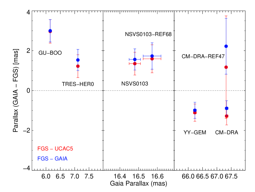
Figure 9: Comparison of FGS parallaxes with Gaia DR2 parallaxes. The red symbols represent residuals from the FGS parallaxes determined from the input spectrophotometric distances and the UCAC5 proper motions while the blue sumbols represent residuals from the FGS parallaxes determined from the input reference star parallaxes and proper motions from Gaia DR2. For more detail, see Section 3.5.

4 Common Proper Motion Pairs

The unanticipated presence of two common proper motion (CPM) companions amongst our reference stars – REF68 for NSVS103, and REF47 for CM Dra – prompted us to seek additional evidence of CPM companions. For the purposes of this paper, our criteria for qualifying as a possible CPM companion was merely agreement at the 3-$\sigma$ level between parallax, and proper motion in both right ascension and declination; these possible CPM companions as indicated by Gaia DR2 data are listed in Table 10. (HST/FGS data were not used for CPM identification since it did not conduct a complete survey of all stars in the vicinity of our target stars.) For YY Gem, its membership in the Castor sextuple system has already been well-established (e.g., Torres & Ribas, 2002, and references therein). For TrES-HER0 and GU Boo, we examined the now-available Gaia DR2 dataset for CPM companions; for the former we found one likely companion, and for the latter, some possibilities.

Table 10: Common proper motion (CPM) companions and possible CPM companions for the eclipsing binaries in our study, as indicated by Gaia DR2 data.

Target	Gaia ID	Sep	Sep	Plx	pmRA	pmDE	typing	Notes
		(arcsec)	(AU)	(mas)	(mas)	(mas)
TrES-Her0	1407718450873494784			$7.113\pm 0.038$	$-12.075\pm 0.070$	$29.904\pm 0.088$
	1407718450873494528	8.2	1148	$7.196\pm 0.069$	$-12.959\pm 0.126$	$30.299\pm 0.158$	$\sim$M5.5V
NSVS0103	1715299716278321408			$16.480\pm 0.030$	$-106.773\pm 0.063$	$58.861\pm 0.051$
	1715287999607537408	65.3	3963	$16.572\pm 0.048$	$-107.709\pm 0.099$	$59.721\pm 0.080$	M4.5V	REF68
CM Dra	1431176943768690816			$67.340\pm 0.051$	$-1113.612\pm 0.114$	$1181.211\pm 0.100$
	1431176943768691328	26.5	394	$67.322\pm 0.023$	$-1110.868\pm 0.048$	$1199.405\pm 0.043$	WD	REF47
GU Boo	1278589709364139520			$6.147\pm 0.016$	$22.728\pm 0.022$	$-30.809\pm 0.031$
	1278514938276783360	2106.8	342563	$6.871\pm 0.755$	$22.061\pm 1.345$	$-30.104\pm 1.574$	unknown	Uncertain CPM
	1278689215165895552	1047.1	170256	$6.111\pm 1.294$	$24.238\pm 2.288$	$-38.721\pm 2.327$	unknown	Uncertain CPM
	1278753639675232128	769.2	125080	$5.956\pm 0.058$	$28.329\pm 0.073$	$-38.046\pm 0.104$	unknown	Uncertain CPM
YY Gem	892348454394856064			$66.232\pm 0.051$	$-201.490\pm 0.087$	$-97.104\pm 0.074$
	No data on Castor	70.4	1063				A1V/? +
	(Gaia bright limit)						A2V/?

Note. — For more details, see Section 4.

4.1 NSVS0103: M Dwarf

NSVS0103-REF68 forms a common proper motion pair with NSVS0103, at an angular distance of 65$\farcs$3. Based on HYDRA spectra for this object, REF68 is a M4.5V star (Fig. 10). The FGS results place the two stars at a distance of around 67 pc, while Gaia DR2 places them at a slightly closer distance of 60.7 pc. From the HST/FGS distance, the linear separation between NSVS0103 and REF68 is 4,400 AU.

4.2 CM Dra: White Dwarf

REF47 associated with CM Dra was previously identified as a white dwarf with a common proper motion (Eggen & Sandage, 1967; Greenstein, 1969), however, we did not realize this when selecting reference stars in the field. The HYDRA data show a nearly featureless spectrum (Fig. 10), consistent with a white dwarf. At the HST/FGS distance of 14.6 pc to CM Dra, its separation of 26$\farcs$5 corresponds to a linear distance of 390 AU. An increasing number of compact companions are being discovered near main sequence stars (e.g., Kane et al., 2019), a population to which this object appears to belong.

Figure 10: WIYN Hydra spectra showing that REF47 for CM Dra is a white dwarf (Section 4.2), and REF 68 for NSVS0103 has a spectral type of M4.5V (Section 4.1). The spectra have not been flattened to remove the spectral continuum nor the instrument response.

4.3 Other CPM data

The Gaia data relating to CPM data for the previous two stars and our other 3 eclipsing binaries can be found in Table 10 (Gaia Collaboration et al., 2016, 2018).

YY Gem’s membership as part of Castor sextuple system is as the lowest mass binary on the outskirts of a much higher mass pair of A-type main sequence stars, each with their own lower mass secondaries. At an angular separation of 70$\farcs$4, at a system distance of 15.1pc this corresponds to a linear distance of 1,060 AU from the close quadruple Castor Aab+Bab.

TrES-Her0 has a CPM companion at 8$\farcs$2 corresponding to a linear separation 1,150 AU. The nature of that companion is unknown; however, with $\Delta$G = 1.8mag, its spectral type will be roughly M5.5V.

The Gaia DR2 for GU Boo does not definitively indicate one or more CPM companions, given the error bars parallax and proper motion for 3 possible CPM candidates. However, these candidates are possibly nearby in $\{\pi,{\rm PM}_{\rm RA},{\rm PM}_{\rm DE}\}$ space, based upon the large errors in their astrometric solutions; the currently reported DR2 values for these objects indicate linear distances from 125,000 to 350,000 AU.

4.4 Discussion

A review of the literature indicates that the presence of CPM pairs to these close binaries is not unexpected. Tokovinin et al. (2006) found a higher order multiplicity fraction of close binaries (e.g. Figure 14 from that study) that indicated most ($\sim$ 63%) had a tertiary component at larger separations. There are several possible formation scenarios that have been proposed for how wide multiple systems such as the ones examined above may have formed. These include the unfolding of triple systems from a protostellar core (Reipurth & Mikkola, 2012), the gravitational binding of stars as a cluster dissolves (Kouwenhoven et al., 2010) and the gravitational binding of stars that form in adjacent protostellar cores (Tokovinin, 2017). While more information is needed to definitively determine the formation mechanism of these pairs, early indications, based on their separations and multiplicity, seem to suggest that systems may have been the result of the unfolding of a triple system in a protostellar core, in particular CM Dra, NSVS0103 and TrES-Her0. This scenario would also allow for the range in outer orbit separations that we see in our systems, which range from $\approx 400-4,000$ AU and are still within the average protostellar core size of 0.1 pc. We caution that this is an extremely small subset of wide pairs which does not explain how the vast majority of wide systems are formed. It is much more likely that wide pairs form through a variety of different mechanisms and it remains to be seen if one dominates over the others.

5 Distance-Enabled Astrophysics

The key results from this study are the mass, luminosity, and radius values for these low-mass stars. We compared our values to similar data products found in Torres et al. (2010); this is of particular interest given their approach was separate but complementary (eclipsing binary orbit fitting) to ours (trignometric parallax combined with SED fitting). Data from the dynamical parallax study of Benedict et al. (2016, B16) are not used here, since absolute luminosities are not determined in B16, just absolute magnitudes $M_{\rm V}$ and $M_{\rm K}$. The techniques presented in this study, particularly the use of binarySED for determination of component true luminosities, would be readily applicable to the objects studied in B16, but this is beyond the scope of the current study.

For the luminosity versus mass and radius versus mass plots (Figures 11 and 12, respectively), it is readily apparent that our distance for GU Boo appears to be incorrect: in both cases, our results and the Torres et al. (2010), aside from GU Boo, are clearly consistent with the relationship fit lines discussed below. Comparing our FGS parallax-derived distance to the distance estimate for GU Boo found in López-Morales & Ribas (2005), there is considerable discrepancy – our FGS value of $313.5\pm 59.0$ pc versus their estimate of $\sim 140$ pc. Gaia DR2 places GU Boo at a distance of 162.6 $\pm$ 0.5 pc. Testing the López-Morales & Ribas (2005) distance in our evaluation of the associated GU Boo parameters of radius and luminosity indicates they converge to values consistent with the fits seen in Figures 11 and 12.

Examining our FGS data, there is no clear cause for this discrepant value: There is no particularly problematic astrometric reference star which, when suppressed, causes the astrometric solution to change substantially. Nor is the target star particularly faint. However, among all of all our targets, GU Boo did have the faintest reference stars, at an average of 0.25-1.0 magnitudes fainter than the other target reference ensembles. It is also one of the most distant astrometric targets, though TrES-Her0 is also at 100+ pc in distance. GU Boo does have the greatest brightness ratio between its two components (Table 6), but this should not affect measurements any more than our other targets: first, the projected angular size of the orbit is small, so astrometric wander due to the bright/dim components is undetectable by Gaia or HST/FGS. Second, the photometric variation of being in/out of eclipse is large for all our science targets (roughly a factor of 50%) and only slightly larger for GU Boo (up to roughly 45%, depending on bandpass).

For completeness, we have kept this object on these plots; however, for the fits described below, we have excluded it from the fitting process.

Mass versus Luminosity. For our target stars, with determined distances $d$ and bolometric fluxes $F_{\rm BOL}$, luminosity is readily established from the familiar relationship $L=4\pi d^{2}F_{\rm BOL}$, with $d$ in cm and $F_{\rm BOL}$ in erg cm^-2 s^-1. We can directly relate these numbers to fractional solar luminosity values using a reference value of $3.83\times 10^{33}$ erg cm^-2 s^-1 for the Sun (Cox, 2000). These results are presented in Figure 11. The resultant luminosity versus mass fit is:

$$\log L=M\times(2.960\pm 0.033)-(2.928\pm 0.012)$$ (1)

We chose the upper bound of 0.65 $M_{\odot}$ for our data which corresponds roughly to the expected ‘turn-on’ point, below which stars become fully convective (Chabrier & Baraffe, 2000). Fitting for the luminosities indicated by the Gaia parallaxes (including GU Boo), the fit in Equation 1 becomes:

$$\log L=M\times(2.920\pm 0.023)-(2.915\pm 0.009)$$ (2)

This is within 1-$\sigma$ of the idealized $L\propto M^{3}$ relationship for this mass range (Eddington, 1924, 1925).

Radius versus Luminosity. Combining distance with estimates of angular size from the SED fitting, linear size is readily inferred. For the sake of clarity, it is worth emphasizing these angular size estimates are simply estimates: the template that the SED fitting process selects as the best-fit template for the input photometry will have an a priori, fixed effective temperature ($T_{\rm EFF}$) value associated with it. From the measured $F_{\rm BOL}$ and that $T_{\rm EFF}$, an angular size can be estimated. This is less direct of an approach to obtaining linear radius than an eclipsing binary orbit solution technique, but it is complementary. These data are presented in Figure 12; as with the previous figure, included in this figure is a fit for stars from our study, excluding GU Boo:

$$R=M\times(0.970\pm 0.012)-(0.030\pm 0.004)$$ (3)

As seen in Figure 12, there are some $\sim 1\sigma$ outliers in radius, in the $M=0.5-0.6M_{\odot}$ range; this mass range has been problematic for angular size estimates and is currently an area of active research (e.g. Mann et al., 2015). As above in Equation 2, a similar fit was established for our program stars, but using radii derived using Gaia parallaxes, inclusive of GU Boo:

$$R=M\times(1.103\pm 0.050)-(0.008\pm 0.021)$$ (4)

This is within 2.5-$\sigma$ of the idealized $R\propto M$ relationship for this mass range (Eddington, 1924, 1925)

The eclipse binary timing of Torres et al. (2010) provides better precision on radius than our approach – and importantly, is a direct rather than indirect measure of radius. However, for those stars (especially single stars) where the system is not eclipsing, this study demonstrates a path forward in at least indirectly assessing the stellar sizes. This is especially appealing in the Gaia DR2 era, where high-precision distances will be available for these objects.

Examining the $R$ versus $M$ fit line extrapolation out to 1 $M_{\odot}$, we see that in relationship to the higher mass points from Torres et al. (2010), this extrapolation appears to agree with the lower bound of the stars in this radius-mass space. It is possible that the objects lurking above the line are beginning to evolve off the main sequence, inflating in size.

Finally, it is worth noting that the SED fitting approach of §3.2 will be of general utility for upcoming Gaia DR2 results. Binaries observed by Gaia will probably be close enough for crude orbit fitting and determination of dynamical parallaxes – e.g. see the reflex motion plots of Benedict et al. (2016) – though with significant complicating factors to be considered. First, the Gaia temporal sampling function convolved with the binary orbital periods will possibly result in serious aliasing of the observed astrometric reflex motion. Second, in some of the unequal brightness cases, while a reflex motion will be detected, the spatial resolution of the instrument is insufficient to spatially separate the two components of a binary, so a robust estimate of that brightness ratio in the Gaia observation bandpass will be necessary. A tool like binarySED will be essential to addressing at least this second concern, and will also be essential for equal brightness ratio binaries.

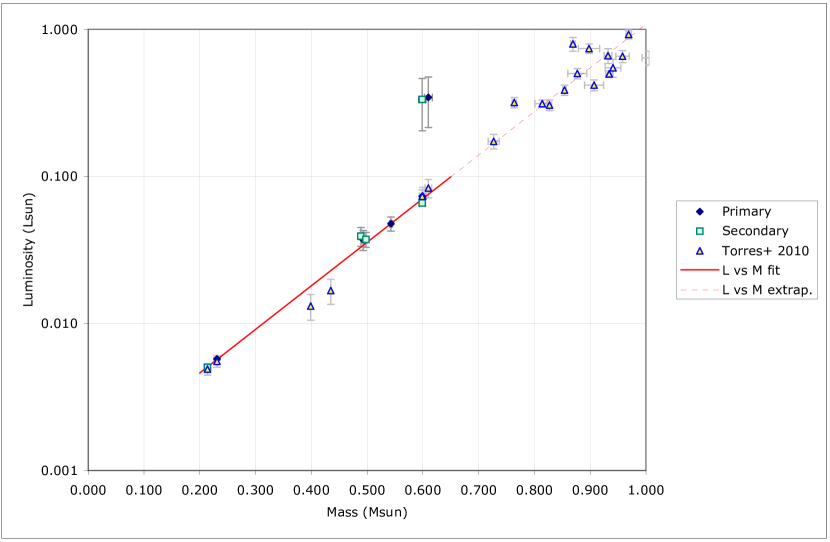
Figure 11: Luminosity versus mass for our target stars, as well as the corresponding points from Torres et al. (2010). The line fit (Eqn. 1) is restricted to the range 0.20 – 0.65 $M_{\odot}$, with an extrapolation of that fit shown to 1.0 $M_{\odot}$. The outlier pair are the GU Boo components – they are not used in calculating the fit shown. For more details, see §5.

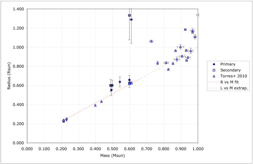
Figure 12: Radius versus mass for our target stars, as well as the corresponding points from Torres et al. (2010). The line fit (Eqn. 3) is restricted to the range 0.20 – 0.65 $M_{\odot}$, with an extrapolation of that fit shown to 1.0 $M_{\odot}$ – as in Fig. 11, the line fit shown does not include the outlier GU Boo. For more details, see §5.

6 Conclusion

For this work, we measured trigonometric parallaxes to five eclipsing binary M-dwarf / M-dwarf systems. By directly determining their distances and using SED fitting to measure their bolometric fluxes, we are able to provide semi-empirical constraints on their physical properties, which are in good agreement with the complementary eclipsing binary values from Torres et al. (2010). Our approach of distance-leveraged SED fitting will be of more general utility for measuring luminosities and inferring linear radii from high-precision distances coming from Gaia since the vast majority of its observed stars will be non-eclipsing binaries or single stars. Finally, provided that robust determination of angular sizes from SED fitting can be made at the 1% level with matching distance precision from Gaia, linear radius discrepancies reported for M-dwarf stars (e.g., Berger et al., 2006; López-Morales, 2007; Lubin et al., 2017) can be straightforwardly investigated with statistically significant samples. These large samples could be correlated with indicators of magnetic activity, rotation rates, multiplicity / proximity of companions, and other phenomena proposed to account for discrepancies in linear radii.

References

- Ballard (2019) Ballard, S. 2019, AJ, 157, 113
- Ballard & Johnson (2016) Ballard, S. & Johnson, J. A. 2016, ApJ, 816, 66
- Benedict et al. (2016) Benedict, G. F., Henry, T. J., Franz, O. G., McArthur, B. E., Wasserman, L. H., Jao, W.-C., Cargile, P. A., Dieterich, S. B., Bradley, A. J., Nelan, E. P., & Whipple, A. L. 2016, AJ, 152, 141
- Benedict et al. (1999) Benedict, G. F., McArthur, B., Chappell, D. W., Nelan, E., Jefferys, W. H., van Altena, W., Lee, J., Cornell, D., Shelus, P. J., Hemenway, P. D., Franz, O. G., Wasserman, L. H., Duncombe, R. L., Story, D., Whipple, A. L., & Fredrick, L. W. 1999, AJ, 118, 1086
- Benedict et al. (2007) Benedict, G. F., McArthur, B. E., Feast, M. W., Barnes, T. G., Harrison, T. E., Patterson, R. J., Menzies, J. W., Bean, J. L., & Freedman, W. L. 2007, AJ, 133, 1810
- Benedict et al. (2002a) Benedict, G. F., McArthur, B. E., Fredrick, L. W., Harrison, T. E., Lee, J., Slesnick, C. L., Rhee, J., Patterson, R. J., Nelan, E., Jefferys, W. H., van Altena, W., Shelus, P. J., Franz, O. G., Wasserman, L. H., Hemenway, P. D., Duncombe, R. L., Story, D., Whipple, A. L., & Bradley, A. J. 2002a, AJ, 123, 473
- Benedict et al. (2002b) Benedict, G. F., McArthur, B. E., Fredrick, L. W., Harrison, T. E., Slesnick, C. L., Rhee, J., Patterson, R. J., Skrutskie, M. F., Franz, O. G., Wasserman, L. H., Jefferys, W. H., Nelan, E., van Altena, W., Shelus, P. J., Hemenway, P. D., Duncombe, R. L., Story, D., Whipple, A. L., & Bradley, A. J. 2002b, AJ, 124, 1695
- Benedict et al. (2017) Benedict, G. F., McArthur, B. E., Nelan, E. P., & Harrison, T. E. 2017, PASP, 129, 012001
- Berger et al. (2006) Berger, D. H., Gies, D. R., McAlister, H. A., ten Brummelaar, T. A., Henry, T. J., Sturmann, J., Sturmann, L., Turner, N. H., Ridgway, S. T., Aufdenberg, J. P., & Mérand, A. 2006, ApJ, 644, 475
- Bond et al. (2013) Bond, H. E., Nelan, E. P., VandenBerg, D. A., Schaefer, G. H., & Harmer, D. 2013, ApJ, 765, L12
- Boyajian et al. (2012) Boyajian, T. S., von Braun, K., van Belle, G., McAlister, H. A., ten Brummelaar, T. A., Kane, S. R., Muirhead, P. S., Jones, J., White, R., Schaefer, G., Ciardi, D., Henry, T., López-Morales, M., Ridgway, S., Gies, D., Jao, W.-C., Rojas-Ayala, B., Parks, J. R., Sturmann, L., Sturmann, J., Turner, N. H., Farrington, C., Goldfinger, P. J., & Berger, D. H. 2012, ApJ, 757, 112
- Butler et al. (2015) Butler, C. J., Erkan, N., Budding, E., Doyle, J. G., Foing, B., Bromage, G. E., Kellett, B. J., Frueh, M., Huovelin, J., Brown, A., & Neff, J. E. 2015, MNRAS, 446, 4205
- Cardelli et al. (1989) Cardelli, J. A., Clayton, G. C., & Mathis, J. S. 1989, ApJ, 345, 245
- Chaboyer et al. (2017) Chaboyer, B., McArthur, B. E., O’Malley, E., Benedict, G. F., Feiden, G. A., Harrison, T. E., McWilliam, A., Nelan, E. P., Patterson, R. J., & Sarajedini, A. 2017, ApJ, 835, 152
- Chabrier & Baraffe (1995) Chabrier, G. & Baraffe, I. 1995, ApJ, 451, L29
- Chabrier & Baraffe (2000) —. 2000, ARA&A, 38, 337
- Coughlin & Shaw (2007) Coughlin, J. L. & Shaw, J. S. 2007, Journal of the Southeastern Association for Research in Astronomy, 1, 7
- Cox (2000) Cox, A. N. 2000, Allen’s astrophysical quantities
- Creevey et al. (2005) Creevey, O. L., Benedict, G. F., Brown, T. M., Alonso, R., Cargile, P., Mandushev, G., Charbonneau, D., McArthur, B. E., Cochran, W., O’Donovan, F. T., Jiménez-Reyes, S. J., Belmonte, J. A., & Kolinski, D. 2005, ApJ, 625, L127
- Delfosse et al. (1999) Delfosse, X., Forveille, T., Mayor, M., Burnet, M., & Perrier, C. 1999, A&A, 341, L63
- Delfosse et al. (2000) Delfosse, X., Forveille, T., Ségransan, D., Beuzit, J.-L., Udry, S., Perrier, C., & Mayor, M. 2000, A&A, 364, 217
- Dressing & Charbonneau (2015) Dressing, C. D. & Charbonneau, D. 2015, ApJ, 807, 45
- Dyck et al. (1996) Dyck, H. M., Benson, J. A., van Belle, G. T., & Ridgway, S. T. 1996, AJ, 111, 1705
- Eddington (1924) Eddington, A. S. 1924, MNRAS, 84, 308
- Eddington (1925) —. 1925, MNRAS, 85, 403
- Eggen & Sandage (1967) Eggen, O. J. & Sandage, A. 1967, ApJ, 148, 911
- Farnham et al. (2000) Farnham, T. L., Schleicher, D. G., & A’Hearn, M. F. 2000, Icarus, 147, 180
- Gaia Collaboration et al. (2018) Gaia Collaboration, Brown, A. G. A., Vallenari, A., Prusti, T., de Bruijne, J. H. J., Babusiaux, C., Bailer-Jones, C. A. L., Biermann, M., Evans, D. W., Eyer, L., & et al. 2018, A&A, 616, A1
- Gaia Collaboration et al. (2016) Gaia Collaboration, Prusti, T., de Bruijne, J. H. J., Brown, A. G. A., Vallenari, A., Babusiaux, C., Bailer-Jones, C. A. L., Bastian, U., Biermann, M., Evans, D. W., & et al. 2016, A&A, 595, A1
- Greenstein (1969) Greenstein, J. L. 1969, ApJ, 158, 281
- Henry (2007) Henry, T. J. 2007, in IAU Symposium, Vol. 240, IAU Symposium, ed. W. I. Hartkopf, E. F. Guinan, & P. Harmanec, 299–299
- Henry et al. (2006) Henry, T. J., Jao, W.-C., Subasavage, J. P., Beaulieu, T. D., Ianna, P. A., Costa, E., & Méndez, R. A. 2006, AJ, 132, 2360
- Jefferys et al. (1988) Jefferys, W. H., Fitzpatrick, M. J., & McArthur, B. E. 1988, Celestial Mechanics, 41, 39
- Johnson (1968) Johnson, H. L. 1968, in Nebulae and Interstellar Matter, ed. B. M. Middlehurst, 167–220
- Kane et al. (2019) Kane, S. R., Dalba, P. A., Horner, J., Li, Z., Wittenmyer, R. A., Horch, E. P., Howell, S. B., & Everett, M. E. 2019, ApJ, 875, 74
- Kouwenhoven et al. (2010) Kouwenhoven, M. B. N., Goodwin, S. P., Parker, R. J., Davies, M. B., Malmberg, D., & Kroupa, P. 2010, MNRAS, 404, 1835
- Landolt (1983) Landolt, A. U. 1983, AJ, 88, 439
- LaSala & Kurtz (1985) LaSala, J. & Kurtz, M. J. 1985, PASP, 97, 605
- Lépine & Shara (2005) Lépine, S. & Shara, M. M. 2005, AJ, 129, 1483
- López-Morales (2007) López-Morales, M. 2007, ApJ, 660, 732
- López-Morales et al. (2006) López-Morales, M., Orosz, J. A., Shaw, J. S., Havelka, L., Arevalo, M. J., McIntyre, T., & Lazaro, C. 2006, ArXiv Astrophysics e-prints
- López-Morales & Ribas (2005) López-Morales, M. & Ribas, I. 2005, ApJ, 631, 1120
- Lubin et al. (2017) Lubin, J. B., Rodriguez, J. E., Zhou, G., Conroy, K. E., Stassun, K. G., Collins, K., Stevens, D. J., Labadie-Bartz, J., Stockdale, C., Myers, G., Colón, K. D., Bento, J., Kehusmaa, P., Petrucci, R., Jofré, E., Quinn, S. N., Lund, M. B., Kuhn, R. B., Siverd, R. J., Beatty, T. G., Harlingten, C., Pepper, J., Gaudi, B. S., James, D., Jensen, E. L. N., Reichart, D., Kedziora-Chudczer, L., Bailey, J., & Melville, G. 2017, ApJ, 844, 134
- Mann et al. (2015) Mann, A. W., Feiden, G. A., Gaidos, E., Boyajian, T., & von Braun, K. 2015, ApJ, 804, 64
- McArthur et al. (2001) McArthur, B. E., Benedict, G. F., Lee, J., van Altena, W. F., Slesnick, C. L., Rhee, J., Patterson, R. J., Fredrick, L. W., Harrison, T. E., Spiesman, W. J., Nelan, E., Duncombe, R. L., Hemenway, P. D., Jefferys, W. H., Shelus, P. J., Franz, O. G., & Wasserman, L. H. 2001, ApJ, 560, 907
- Metcalfe et al. (1996) Metcalfe, T. S., Mathieu, R. D., Latham, D. W., & Torres, G. 1996, ApJ, 456, 356
- Morales et al. (2009) Morales, J. C., Ribas, I., Jordi, C., Torres, G., Gallardo, J., Guinan, E. F., Charbonneau, D., Wolf, M., Latham, D. W., Anglada-Escudé, G., Bradstreet, D. H., Everett, M. E., O’Donovan, F. T., Mandushev, G., & Mathieu, R. D. 2009, ApJ, 691, 1400
- Nelan (2012) Nelan, E. 2012, Fine Guidance Sensor Instrument Handbook for Cycle 21 v.20.0
- Nelan & Bond (2013) Nelan, E. P. & Bond, H. E. 2013, ApJ, 773, L26
- Ochsenbein et al. (2000) Ochsenbein, F., Bauer, P., & Marcout, J. 2000, A&AS, 143, 23
- Perryman et al. (1997) Perryman, M. A. C., Lindegren, L., Kovalevsky, J., Hoeg, E., Bastian, U., Bernacca, P. L., Crézé, M., Donati, F., Grenon, M., van Leeuwen, F., van der Marel, H., Mignard, F., Murray, C. A., Le Poole, R. S., Schrijver, H., Turon, C., Arenou, F., Froeschlé, M., & Petersen, C. S. 1997, A&A, 323, L49
- Pickles (1998) Pickles, A. J. 1998, PASP, 110, 863
- Reipurth & Mikkola (2012) Reipurth, B. & Mikkola, S. 2012, Nature, 492, 221
- Ribas (2003) Ribas, I. 2003, A&A, 398, 239
- Roeser et al. (2010) Roeser, S., Demleitner, M., & Schilbach, E. 2010, AJ, 139, 2440
- Soderblom et al. (2005) Soderblom, D. R., Nelan, E., Benedict, G. F., McArthur, B., Ramirez, I., Spiesman, W., & Jones, B. F. 2005, AJ, 129, 1616
- Tokovinin (2017) Tokovinin, A. 2017, MNRAS, 468, 3461
- Tokovinin et al. (2006) Tokovinin, A., Thomas, S., Sterzik, M., & Udry, S. 2006, A&A, 450, 681
- Torres et al. (2010) Torres, G., Andersen, J., & Giménez, A. 2010, A&A Rev., 18, 67
- Torres & Ribas (2002) Torres, G. & Ribas, I. 2002, ApJ, 567, 1140
- Turnbull & Tarter (2003) Turnbull, M. C. & Tarter, J. C. 2003, ApJS, 149, 423
- van Altena et al. (1995) van Altena, W. F., Lee, J. T., & Hoffleit, D. 1995, VizieR Online Data Catalog, 1174, 0
- VandenBerg et al. (2014) VandenBerg, D. A., Bond, H. E., Nelan, E. P., Nissen, P. E., Schaefer, G. H., & Harmer, D. 2014, ApJ, 792, 110
- von Braun & Boyajian (2017) von Braun, K. & Boyajian, T. 2017, ArXiv e-prints
- von Braun et al. (2014) von Braun, K., Boyajian, T. S., van Belle, G. T., Kane, S. R., Jones, J., Farrington, C., Schaefer, G., Vargas, N., Scott, N., ten Brummelaar, T. A., Kephart, M., Gies, D. R., Ciardi, D. R., López-Morales, M., Mazingue, C., McAlister, H. A., Ridgway, S., Goldfinger, P. J., Turner, N. H., & Sturmann, L. 2014, MNRAS, 438, 2413
- Wenger et al. (2000) Wenger, M., Ochsenbein, F., Egret, D., Dubois, P., Bonnarel, F., Borde, S., Genova, F., Jasniewicz, G., Laloë, S., Lesteven, S., & Monier, R. 2000, A&AS, 143, 9
- Zacharias et al. (2017) Zacharias, N., Finch, C., & Frouard, J. 2017, AJ, 153, 166
- Zacharias et al. (2015) Zacharias, N., Finch, C., Subasavage, J., Bredthauer, G., Crockett, C., Divittorio, M., Ferguson, E., Harris, F., Harris, H., Henden, A., Kilian, C., Munn, J., Rafferty, T., Rhodes, A., Schultheiss, M., Tilleman, T., & Wieder, G. 2015, AJ, 150, 101
- Zacharias et al. (2013) Zacharias, N., Finch, C. T., Girard, T. M., Henden, A., Bartlett, J. L., Monet, D. G., & Zacharias, M. I. 2013, AJ, 145, 44