On the Riemann-Hilbert problem for the Chen-Lee-Liu derivative nonlinear Schrödinger equation

Abstract

In this work, we investigated a combined Chen-Lee-Liu derivative nonlinear Schrödinger equation(called CLL-NLS equation by Kundu) on the half-line by unified transformation approach. We gives spectral analysis of the Lax pair for CLL-NLS equation, and establish a matrix Riemann-Hilbert problem, so as to reconstruct the solution $r(z,t)$ of the CLL-NLS equation by solving. Furthermore, the spectral functions are not independent, but enjoy by a compatibility condition, which is the so-called global relation.

1 Introduction

As we all know, the nonlinear Schrödinger(NLS) equation and the derivative NLS(DNLS) equation are all important equations in the field of mathematical physics. On the one hand, the NLS equation[1]

$$ir_{t}+r_{zz}\pm|r|^{2}r=0,$$ (1.1)

can be used to describe the movement of microscopic particles, and is also one of the basic equations of quantum mechanics. In quantum mechanics, the solution of particle problems is usually converted into the solution of the stationary NLS equation problem. On the other hand, there are three types of DNLS equation, the first is the famous Kaup-Newell equation[2], also known as DNLS-I equation

$$r_{t}+r_{zz}\pm i(|r|^{2}r)_{z}=0,$$ (1.2)

the second is Chen-Lee-Liu equation[3], also known as DNLS-II equation

$$ir_{t}+r_{zz}-i|r|^{2}r_{x}=0,$$ (1.3)

and the last is Gerdjikov-Ivanov equation[4], also known as DNLS-III equation

$$ir_{t}+r_{zz}-i|r|^{2}\bar{r}_{x}+\frac{1}{2}|r|^{4}r=0.$$ (1.4)

The DNLS type equation has important applications in nonlinear optics and plasma physics. It can be used not only to describe picosecond pulse in single-mode nonlinear fiber, but also to control the evolution of small amplitude Alfvén waves or large amplitude magnetohydrodynamic(MHD) waves in plasmas.

With the in-depth study of soliton theory, a unified transformation(UT) approach to solve the initial-boundary value problems(IBVPs) of integrable model is proposed by Fokas[5], also known as the Fokas approach. Since the UT approach have been proposed, the IBVPs of many nonlinear integrable models have been extensively studied[6, 7, 8, 9, 10, 11, 12, 13, 14, 15, 16, 17, 18, 19, 20]. In particular, Fokas et al. analyzed the IBVPs of the NLS equation(1.1) on the half-line[21], Monvel et al. gives the IBVPs on a finite interval case[22]. Lenells discussed the IBVPs of the Kaup-Newell(DNLS-I) equation(1.2) on the half-line [23], Xu and Fan gives the IBVPs on a finite interval case[24]. Zhang et al. studied the IBVPs of the Chen-Lee-Liu(DNLS-II) equation(1.3) on the half-line[25]. Zhu et al. investigated the IBVPs of the Gerdjikov-Ivanov(DNLS-III) equation(1.4) on the half-line[26], and then gives the IBVPs on a finite interval[27].

In 1984, Kundu[28] proposed a combined Chen-Lee-Liu derivative nonlinear Schrödinger equation (called CLL-NLS equation by Kundu)

$$ir_{t}+r_{zz}+|r|^{2}r-|r|^{2}r_{z}=0.$$ (1.5)

which is a completely integrable model. In fact, the CLL-NLS equation(1.5) can be derived from the modified NLS equation(also known as the Dysthe equation) which ignores the mean flow term in hydrodynamics[29]. In 2014, Chan et al. give the rogue wave of the CLL-NLS equation(1.5) based on the Hirota bilinear transformation, and pointed out that the CLL-NLS model can be explain the experimental phenomena in nonlinear optical fibers and water wave flumes[30]. Especially, Zhang et al. obtain higher-order solutions of the CLL-NLS equation(1.5) by using the Darboux transformation method[31], includes non-vanishing boundary solitons, breathers and rogue wave solutions. In this paper, let $(z,t)\in\Gamma=\{(z,t)|0<z<\infty,0<t<T\}$, we aim to investigate the IBVPs of the CLL-NLS equation(1.5) via UT approach.

The paper is organized as follows. Section 2, we will gives spectral analysis of the Lax pair for (1.5). Section 3, some key functions $u(\varsigma),v(\varsigma),U(\varsigma),V(\varsigma)$ are further analyzed. Section 4, the Riemann-Hilbert problem is proposed. Section 5 are some conclusions and discussions.

2 The spectral analysis

The Lax pair for CLL-NLS equation (1.5) as follows[31, 32, 33]

$$\Psi_{z}=M(z,t,\varsigma)\Psi=(i\sigma\varsigma^{2}-\frac{1}{2}i\sigma+R\varsigma+\frac{1}{2}iR^{2}\sigma)\Psi,$$ (2.1a)

$$\Psi_{t}=N(z,t,\varsigma)\Psi=[-2i(\varsigma^{2}-\frac{1}{2})^{2}\sigma-2R\varsigma^{3}-iR^{2}\sigma\varsigma^{2}+(R+i\sigma R_{z}-\frac{1}{2}R^{3})\varsigma$$

$$\qquad\qquad\qquad\quad-\frac{1}{8}iR^{4}\sigma+\frac{1}{4}(RR_{z}-R_{z}R)]\Psi,$$ (2.1b)

with

$$\Psi(z,t,\varsigma)=\left(\begin{array}[]{c}\Psi_{1}(z,t,\varsigma)\\ \Psi_{2}(z,t,\varsigma)\end{array}\right),\sigma=\left(\begin{array}[]{cc}1&0\\ 0&-1\end{array}\right),R=\left(\begin{array}[]{cc}0&r\\ -\bar{r}&0\end{array}\right).$$ (2.2)

2.1 The exact 1-form

The Lax pair Eq.(2.1a)-(2.1b) rewrite as

$$\Psi_{z}-i(\varsigma^{2}-\frac{1}{2})\sigma\Psi=A\Psi,$$ (2.3a)

$$\Psi_{t}+2i(\varsigma^{2}-\frac{1}{2})^{2}\sigma\Psi=B\Psi,$$ (2.3b)

where the complex number $\varsigma$ is a associated spectral parameter and

$$A=R\varsigma+\frac{1}{2}iR^{2}\sigma,\,B=-2R\varsigma^{3}-iR^{2}\sigma\varsigma^{2}+(R+i\sigma R_{z}-\frac{1}{2}R^{3})\varsigma-\frac{1}{8}iR^{4}\sigma+\frac{1}{4}(RR_{z}-R_{z}R).$$

Let’s do the first function transformation $\Phi(z,t,\varsigma)$ as follows

$$\Phi(z,t,\varsigma)=\Psi(z,t,\varsigma)e^{[-i(\varsigma^{2}-\frac{1}{2})z+2i(\varsigma^{2}-\frac{1}{2})^{2}t]\sigma},0<x<\infty,0<t<T.$$ (2.4)

Hence, Eq.(2.3a)-(2.3b) equal to

$$\Phi_{z}-i(\varsigma^{2}-\frac{1}{2})[\sigma,\Phi]=A\Phi,$$ (2.5a)

$$\Phi_{t}+2i(\varsigma^{2}-\frac{1}{2})^{2}[\sigma,\Phi]=B\Phi,$$ (2.5b)

where $[\sigma,\Phi]=\sigma\Phi-\Phi\sigma$. It is not difficult to find that the above equations satisfies a full differential form

$$d(e^{[-i(\varsigma^{2}-\frac{1}{2})z+2i(\varsigma^{2}-\frac{1}{2})^{2}t]\bar{\sigma}}\Phi(z,t,\varsigma))=e^{[-i(\varsigma^{2}-\frac{1}{2})z+2i(\varsigma^{2}-\frac{1}{2})^{2}t]\bar{\sigma}}(Adz+Bdt)\Phi(z,t,\varsigma),$$ (2.6)

where $\hat{\sigma}$ represents a matrix operator (see [20]).

One assume that the solution of Eq.(2.5a)-(2.5b) enjoy the following asymptotic expansion form We suppose that the following asymptotic expansion

$$\Phi(z,t,\varsigma)=Q_{0}+\frac{Q_{1}}{\varsigma}+\frac{Q_{2}}{\varsigma^{2}}+\frac{Q_{3}}{\varsigma^{3}}+O(\frac{1}{\varsigma^{4}}),\varsigma\rightarrow\infty.$$ (2.7)

one substituting Eq.(2.7) into Eq.(2.5a) and Eq.(2.5b), respectively, and comparing the coefficient for $\varsigma$ gives rise to

$$Q_{0z}=\frac{1}{4}i|r|^{2}\sigma Q_{0},$$ (2.8a)

$$Q_{0t}=(\frac{1}{8}|r|^{4}+\frac{1}{4}(\bar{r}r_{z}-r\bar{r}_{z}))\sigma Q_{0}.$$ (2.8b)

Owing to Eq.(2.1a)-(2.1b) admits the conservation laws as follows

$$(i|r|^{2})_{t}=(\frac{1}{2}i|r|^{4}+(\bar{r}r_{z}-r\bar{r}_{z}))_{z}.$$

then, one can define

$$Q_{0}(z,t)=e^{i\int_{(\infty,0)}^{(z,t)}\Theta(z,t)\sigma},$$ (2.9)

where $\Theta$ is the exact closed 1-form defined by

$$\Theta(z,t)=\Theta_{1}dz+\Theta_{2}dt=\frac{1}{4}|r|^{2}dx+(\frac{1}{8}|r|^{4}-\frac{1}{4}i(\bar{r}r_{z}-r\bar{r}_{z}))dt.$$ (2.10)

As a result of Eq.(2.9) is independent of the integration path and $\Theta$ is independent of $\varsigma$, one can take the second function transformation $H(z,t,\varsigma)$

$$\Phi(z,t,\varsigma)=e^{i\int_{(0,0)}^{(z,t)}\Theta\hat{\sigma}}H(z,t,\varsigma)Q_{0}(z,t).$$ (2.11)

thus, Eq.(2.6) become to

$$d(e^{[-i(\varsigma^{2}-\frac{1}{2})z+2i(\varsigma^{2}-\frac{1}{2})^{2}t]\hat{\sigma}}H(z,t,\varsigma))=J(z,t,\varsigma),$$ (2.12)

where

$$J(z,t,\varsigma)=e^{[-i(\varsigma^{2}-\frac{1}{2})z+2i(\varsigma^{2}-\frac{1}{2})^{2}t]\hat{\sigma}}F(z,t,\varsigma)H(z,t,\varsigma),$$ (2.13a)

$$F(z,t,\varsigma)=A_{1}(z,t,\varsigma)dz+B_{1}(z,t,\varsigma)dt=e^{-i\int_{(0,0)}^{(z,t)}\Theta\hat{\sigma}}(Adz+Bdt-i\Theta\sigma).$$ (2.13b)

where $A(z,t,\varsigma),B(z,t,\varsigma)$ and $\Theta$ given by

$$A_{1}(z,t,\varsigma)=\left(\begin{array}[]{cc}-\frac{3i}{4}|r|^{2}&\varsigma re^{2i\int_{(0,0)}^{(z,t)}\Theta}\\ -\varsigma\bar{r}qe^{-2i\int_{(0,0)}^{(z,t)}\Theta}&\frac{3i}{4}|r|^{2}\end{array}\right),$$ (2.14c)

$$B_{1}(z,t,\varsigma)=\left(\begin{array}[]{cc}-\frac{i}{4}|r|^{4}+\frac{5}{4}(\bar{r}r_{z}-\bar{r}_{z}r)&(-2\varsigma^{3}r+i\varsigma^{2}|r|^{2}+\varsigma(r_{z}+r-|r|^{2}r))e^{2i\int_{(0,0)}^{(z,t)}\Theta}\\ (2\varsigma^{3}\bar{r}-i\varsigma^{2}|r|^{2}+\varsigma(\bar{r}_{z}-\bar{r}+|r|^{2}\bar{r}))e^{-2i\int_{(0,0)}^{(z,t)}\Theta}&\frac{i}{4}|r|^{4}-\frac{5}{4}(\bar{r}r_{z}-\bar{r}_{z}r)\end{array}\right).$$ (2.14f)

Then Eq.(2.12) equal to

$$H_{x}-i(\varsigma^{2}-\frac{1}{2})[\sigma,H]=A_{1}H,$$ (2.15a)

$$H_{t}+2i(\varsigma^{2}-\frac{1}{2})^{2}[\sigma,H]=B_{1}H.$$ (2.15b)

2.2 The analytic and bounded eigenfunctions $\{H_{j}(z,t,\varsigma)\}_{1}^{3}$

Set that $r(z,t)\in\mathcal{S},((z,t)\in\Gamma)$, one enjoy three eigenfunctions $\{H_{j}(z,t,\varsigma)\}_{1}^{3}$ of Eq.(2.15a)-(2.15b) defined by following integral equation

$$H_{j}(z,t,\varsigma)=\mathrm{I}+\int_{(z_{j},t_{j})}^{(z,t)}e^{[i(\varsigma^{2}-\frac{1}{2})z-2i(\varsigma^{2}-\frac{1}{2})^{2}t]\hat{\sigma}}J(\zeta,\tau,\varsigma),$$ (2.16)

where $(z_{1},t_{1})=(0,0),(z_{2},t_{2})=(0,T),(z_{3},t_{3})=(\infty,t)$. Since Eq.(2.16) has nothing to do with the integral path, one choose the integration path shown in Figure 1, then, one get

$$H_{1}(z,t,\varsigma)=\mathrm{I}+\int_{0}^{z}e^{i(\varsigma^{2}-\frac{1}{2})(z-\zeta)\hat{\sigma}}(A_{1}H_{1})(\zeta,t,\varsigma)d\zeta$$

$$\qquad\qquad\qquad+e^{i(\varsigma^{2}-\frac{1}{2})z\hat{\sigma}}\int_{0}^{t}e^{-2i(\varsigma^{2}-\frac{1}{2})^{2}(t-\tau)\hat{\sigma}}(B_{1}H_{1})(0,\tau,\varsigma)d\tau,$$ (2.17a)

$$H_{2}(z,t,\varsigma)=\mathrm{I}+\int_{0}^{z}e^{i(\varsigma^{2}-\frac{1}{2})(z-\zeta)\hat{\sigma}}(A_{1}H_{2})(\zeta,t,k)d\zeta$$

$$\qquad\qquad\qquad-e^{-i(\varsigma^{2}-\frac{1}{2})z\hat{\sigma}}\int_{t}^{T}e^{-2i(\varsigma^{2}-\frac{1}{2})^{2}(t-\tau)\hat{\sigma}_{3}}(B_{1}H_{2})(0,\tau,\varsigma)d\tau,$$ (2.17b)

$$H_{3}(z,t,\varsigma)=\mathrm{I}-\int_{z}^{\infty}e^{i(\varsigma^{2}-\frac{1}{2})(z-\zeta)\hat{\sigma}3}(A_{1}H_{3})(\zeta,t,\varsigma)d\zeta.$$ (2.17c)

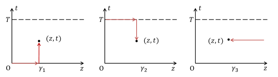
Figure 1: The smooth curve $\gamma_{1},\gamma_{2},\gamma_{3}$ in the $(z,t)$-plan

Besides, the following equation holds on the $(x,t)$ plan

$$\gamma_{1}=(z_{1},t_{1})\rightarrow(z,t):z-\zeta\geq 0,t-\tau\geq 0,$$ (2.18a)

$$\gamma_{2}=(z_{2},t_{2})\rightarrow(z,t):z-\zeta\geq 0,t-\tau\leq 0,$$ (2.18b)

$$\gamma_{3}=(z_{3},t_{3})\rightarrow(z,t):z-\zeta\leq 0.$$ (2.18c)

In order to obtain the bounded analytical region of $\{H_{j}(z,t,\varsigma)\}_{1}^{3}$ on the complex $\varsigma$-plane, one use curve

$$\Omega(\varsigma)=\{\varsigma\in\mathbb{C}|\mathrm{Re}(\phi(\varsigma))\mathrm{Re}(\psi(\varsigma))=0,\phi(\varsigma)=i(\varsigma^{2}-\frac{1}{2}),\psi(\varsigma)=2i(\varsigma^{2}-\frac{1}{2})^{2}\},$$

to divide the complex $\varsigma$-plane as shown in Figure 2. Thus, we get

$$\begin{array}[]{l}D_{1}=\{\varsigma\in\mathbb{C}|\mathrm{Re}\phi(\varsigma)>0\,\,and\,\,\mathrm{Re}\psi(\varsigma)>0\},\\ D_{2}=\{\varsigma\in\mathbb{C}|\mathrm{Re}\phi(\varsigma)>0\,\,and\,\,\mathrm{Re}\psi(\varsigma)<0\},\\ D_{3}=\{\varsigma\in\mathbb{C}|\mathrm{Re}\phi(\varsigma)<0\,\,and\,\,\mathrm{Re}\psi(\varsigma)<0\},\\ D_{4}=\{\varsigma\in\mathbb{C}|\mathrm{Re}\phi(\varsigma)<0\,\,and\,\,\mathrm{Re}\psi(\varsigma)>0\}.\end{array}$$ (2.23)

Furthermore, the bounded analysis area of $\{H_{j}(z,t,\varsigma)\}_{1}^{3}$ as follows

$$H_{1}(z,t,\varsigma):\,(\phi_{-}\cap\psi_{+},\phi_{+}\cap\psi_{-})=:(D_{4},D_{2}),$$ (2.24a)

$$H_{2}(z,t,\varsigma):\,(\phi_{-}\cap\psi_{-},\phi_{+}\cap\psi_{+})=:(D_{3},D_{1}),$$ (2.24b)

$$H_{3}(z,t,\varsigma):\,(\phi_{+},\,\phi_{-})=:(D_{1}\cup D_{2},D_{3}\cup D_{4}),$$ (2.24c)

where $\phi_{+}=:\mathrm{Re}\phi(\varsigma)>0$, $\phi_{-}=:\mathrm{Re}\phi(\varsigma)<0$, $\psi_{+}=:\mathrm{Re}\psi(\varsigma)>0$, $\psi_{-}=:\mathrm{Re}\psi(\varsigma)<0$.

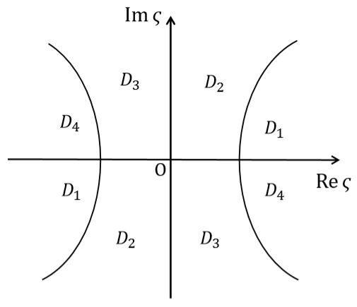
Figure 2: The areas $D_{i},i=1,\ldots,4$ division on the complex $\varsigma$-plane

To construct the Riemann-Hilbert problem of CLL-NLS equation (1.5), one also need to define two important special functions $w(\varsigma)$ and $W(\varsigma)$ by:

$$H_{3}(z,t,\varsigma)=H_{1}(z,t,\varsigma)e^{[i(\varsigma^{2}-\frac{1}{2})z-2i(\varsigma^{2}-\frac{1}{2})^{2}t]\hat{\sigma}}w(\varsigma),$$ (2.25a)

$$H_{2}(z,t,\varsigma)=H_{1}(z,t,\varsigma)e^{[i(\varsigma^{2}-\frac{1}{2})z-2i(\varsigma^{2}-\frac{1}{2})^{2}t])\hat{\sigma}}W(\varsigma).$$ (2.25b)

Upon evaluation at $(z,t)=(0,0)$ and $(z,t)=(0,T)$, respectively, Eq.(2.25a) and Eq.(2.25b) yields

$$W^{-1}(\varsigma)=e^{-2i(\varsigma^{2}-\frac{1}{2})^{2}T\hat{\sigma}}H_{1}(0,T,\varsigma),w(\varsigma)=H_{3}(0,0,\varsigma),$$ (2.26)

According to (2.25a)-(2.25b) and Eq.(2.26), one have

$$H_{2}(z,t,\varsigma)=H_{3}(z,t,\varsigma)e^{[i(\varsigma^{2}-\frac{1}{2})z-2i(\varsigma^{2}-\frac{1}{2})^{2}t]\hat{\sigma}}(w(\varsigma))^{-1}W(\varsigma),$$ (2.27)

Especially, if one remember that $[H_{j}]_{k}(z,t,\varsigma)$ denotes $k$-columns of $H_{j}(z,t,\varsigma)$, one obtain $H_{1}(z,t,\varsigma),H_{2}(z,t,\varsigma)$ at $z=0$

$$H_{1}(0,t,\varsigma)=([H_{1}]_{1}^{D_{1}\cup D_{4}}(0,t,\varsigma),[H_{1}]_{2}^{D_{2}\cup D_{3}}(0,t,\varsigma))$$

$$\qquad\qquad\,=\mathrm{I}+\int_{0}^{t}e^{-2i(\varsigma^{2}-\frac{1}{2})^{2}(t-\tau)\hat{\sigma}}(B_{1}H_{1})(0,\tau,\varsigma)d\tau,$$ (2.28a)

$$H_{2}(0,t,\varsigma)=([H_{2}]_{1}^{D_{2}\cup D_{3}}(0,t,\varsigma),[H_{2}]_{2}^{D_{1}\cup D_{4}}(0,t,\varsigma))$$

$$\qquad\qquad\,=\mathrm{I}-\int_{t}^{T}e^{-2i(\varsigma^{2}-\frac{1}{2})^{2}(t-\tau)\hat{\sigma}}(B_{1}H_{2})(0,\tau,\varsigma)d\tau,$$ (2.28b)

and $H_{1}(z,t,\varsigma),H_{3}(z,t,\varsigma)$ at $t=0$.

$$H_{1}(z,0,\varsigma)=([H_{1}]_{1}^{D_{3}\cup D_{4}}(z,0,\varsigma),[H_{1}]_{2}^{D_{1}\cup D_{2}}(z,0,\varsigma))$$

$$\qquad\qquad\,=\mathrm{I}+\int_{0}^{z}e^{i(\varsigma^{2}-\frac{1}{2})(z-\zeta)\hat{\sigma}}(A_{1}H_{1})(\zeta,0,k)d\zeta,$$ (2.29a)

$$H_{3}(z,0,\varsigma)=([H_{3}]_{1}^{D_{1}\cup D_{2}}(z,0,\varsigma),[H_{3}]_{2}^{D_{3}\cup D_{4}}(z,0,\varsigma))$$

$$\qquad\qquad\,=\mathrm{I}-\int_{z}^{\infty}e^{i(\varsigma^{2}-\frac{1}{2})(z-\zeta)\hat{\sigma}}(A_{1}H_{3})(\zeta,0,\varsigma)d\zeta,$$ (2.29b)

where $H_{j}^{D_{i}}$ represents the bounded analytic region of $\{H_{j}\}_{1}^{3}$ is $\varsigma\in D_{i},i=1,2,3,4$.

Set that $r_{0}(z)=r(z,t=0)$, $s_{0}(t)=r(z=0,t)$, $s_{1}(t)=r_{z}(z=0,t)$ are initial data and boundary datas of $r(z,t)$ and $r_{z}(z,t)$, then, one yields

$$A_{1}(z,0,\varsigma)=\left(\begin{array}[]{cc}-\frac{3i}{4}|r_{0}|^{2}&\varsigma r_{0}e^{\frac{i}{2}\int_{0}^{z}|r_{0}|^{2}dz}\\ \varsigma\bar{r}_{0}e^{-\frac{i}{2}\int_{0}^{z}|r_{0}|^{2}dz}&\frac{3i}{4}|r_{0}|^{2}\end{array}\right),$$ (2.30c)

$$B_{1}(0,t,\varsigma)=\left(\begin{array}[]{cc}-\frac{i}{4}|s_{0}|^{4}+\frac{5}{4}(\bar{s}_{0}s_{1}-\bar{s}_{1}s_{0})&B_{12}^{(1)}(0,t,\varsigma)\\ B_{21}^{(1)}(0,t,\varsigma)&\frac{i}{4}|s_{0}|^{4}-\frac{5}{4}(\bar{s}_{0}s_{1}-\bar{s}_{1}s_{0})\end{array}\right).$$ (2.30f)

with

$$B_{12}^{(1)}(0,t,\varsigma)=(-2\varsigma^{3}s_{0}+i\varsigma^{2}|s_{0}|^{2}+\varsigma(s_{1}+s_{0}-|s_{0}|^{2}s_{0}))e^{\int_{0}^{t}(\frac{i}{4}|s_{0}|^{4}+\frac{1}{2}(\bar{s}_{0}s_{1}-s_{0}\bar{s}_{1}))dt},$$

$$B_{21}^{(1)}(0,t,\varsigma)=(2\varsigma^{3}\bar{s}_{0}-i\varsigma^{2}|s_{0}|^{2}+\varsigma(\bar{s}_{1}-\bar{s}_{0}+|s_{0}|^{2}\bar{s}_{1}))e^{-\int_{0}^{t}(\frac{i}{4}|s_{0}|^{4}+\frac{1}{2}(\bar{s}_{0}s_{1}-s_{0}\bar{s}_{1}))dt}$$

2.3 The other properties of the eigenfunctions

Proposition 2.1

The functions $H_{j}(z,t,\varsigma)=([H_{j}]_{1}(z,t,\varsigma),[H_{j}]_{2}(z,t,\varsigma)),j=1,2,3,$ possess the following properties

• $\mathrm{det}H_{j}(z,t,\varsigma)=1,j=1,2,3$,

• $[H_{1}]_{1}(z,t,\varsigma)$ is analytic for $\varsigma\in D_{4}$, and continues to $\bar{D}_{4},[H_{1}]_{2}(z,t,\varsigma)$ is analytic for $\varsigma\in D_{2}$, and continues to $\bar{D}_{2}$.

• $[H_{2}]_{1}(z,t,\varsigma)$ is analytic for $\varsigma\in D_{3}$, and continues to $\bar{D}_{3},[H_{2}]_{2}(z,t,\varsigma)$ is analytic for $\varsigma\in D_{1}$, and continues to $\bar{D}_{1}$.

• $[H_{3}]_{1}(z,t,\varsigma)$ is analytic for $\varsigma\in D_{1}\cup D_{2}$, and continues to $\bar{D}_{1}\cup\bar{D}_{2},[H_{3}]_{2}(z,t,\varsigma)$ is analytic for $\varsigma\in D_{3}\cup D_{4}$, and continues to $\bar{D}_{3}\cup\bar{D}_{4}$.

• As $\varsigma\rightarrow\infty$, $[H_{j}]_{1}(z,t,\varsigma)\rightarrow(1,0)^{T}$, $[H_{j}]_{2}(z,t,\varsigma)\rightarrow(0,1)^{T}.$

Proposition 2.2

According to Eq.(2.26), one find that $w(\varsigma),W(\varsigma)$ can be expressed by

$$w(\varsigma)=\mathrm{I}-\int_{0}^{\infty}e^{-i(\varsigma^{2}-\frac{1}{2})(\zeta-z)\hat{\sigma}}(A_{1}H_{3})(\zeta,0,\varsigma)d\zeta,$$ (2.31a)

$$W^{-1}(\varsigma)=\mathrm{I}+\int_{0}^{T}e^{2i(\varsigma^{2}-\frac{1}{2})^{2}(\tau-t)\hat{\sigma}}(B_{1}H_{1})(0,\tau,\varsigma)d\tau.$$ (2.31b)

Assume that $w(\varsigma),W(\varsigma)$ admits the following $2\times 2$ matrix from

$$w(\varsigma)=\left(\begin{array}[]{cc}\overline{u(\bar{\varsigma})}&v(\varsigma)\\ \overline{v(\bar{\varsigma})}&u(\varsigma)\end{array}\right),W(\varsigma)=\left(\begin{array}[]{cc}\overline{U(\bar{\varsigma})}&V(\varsigma)\\ \overline{V(\bar{\varsigma})}&U(\varsigma)\\ \end{array}\right).$$ (2.36)

It follows from Eq.(2.26) and Eqs.(2.31a)-(2.31b) that the following key properties are ture:

• $$(v(\varsigma),u(\varsigma))^{T}=[H_{3}]_{2}^{D_{1}\cup D_{2}}(0,0,\varsigma),\quad(-e^{2i(\varsigma^{2}-\frac{1}{2})^{2}T}V(\varsigma),\overline{U(\bar{\varsigma})})^{T}=[H_{1}]_{2}^{D_{2}\cup D_{4}}(0,t,\varsigma).$$

• $$u(-\varsigma)=u(\varsigma),\,\,v(-\varsigma)=-v(\varsigma),\,\,U(-\varsigma)=U(\varsigma),\,\,V(-\varsigma)=-V(\varsigma).$$

• $$For\,\,\varsigma\in\mathrm{R},\quad\mathrm{det}w(\varsigma)=1,\quad for\,\,\varsigma\in\mathrm{C}\,\,(\mathrm{Im}(\varsigma^{2}-\frac{1}{2})^{2}=0,\,if\,T=\infty),\,\,\mathrm{det}W(\varsigma)=1.$$

• $$As\,\varsigma\rightarrow\infty,\,u(\varsigma)=1+\mathrm{O}(\varsigma^{-1}),\,\,v(\varsigma)=\mathrm{O}(\varsigma^{-1}),\,\,U(k)=1+\mathrm{O}(\varsigma^{-1}),\,\,V(\varsigma)=\mathrm{O}(\varsigma^{-1}).$$

2.4 The basic Riemann-Hilbert problem

For the convenience of calculation, one introduce the following symbol description

$$\eta(\varsigma)=-(\varsigma^{2}-\frac{1}{2})z+2(\varsigma^{2}-\frac{1}{2})^{2}t,\,\beta(\varsigma)=u(\varsigma)\overline{U(\bar{\varsigma})}+v(\varsigma)\overline{V(\bar{\varsigma})},\,\delta(\varsigma)=\frac{v(\varsigma)}{\overline{u(\bar{\varsigma})}},\,\Delta(\varsigma)=-\frac{\overline{V(\bar{\varsigma})}}{u(\varsigma)\beta(\varsigma)},$$ (2.37)

and the $E(z,t,\varsigma)$ defined by

$$E_{+}(z,t,\varsigma)=([H_{3}]_{1}^{D_{1}\cup D_{2}}(z,t,\varsigma),\frac{[H_{2}]_{2}^{D_{1}}(z,t,\varsigma)}{\overline{\beta(\bar{\varsigma})}}),\varsigma\in D_{1},$$ (2.38a)

$$E_{-}(z,t,\varsigma)=([H_{3}]_{1}^{D_{1}\cup D_{2}}(z,t,\varsigma),\frac{[H_{1}]_{2}^{D_{2}}(z,t,\varsigma)}{\overline{u(\bar{\varsigma})}}),\varsigma\in D_{2},$$ (2.38b)

$$E_{-}(z,t,\varsigma)=(\frac{[H_{2}]_{1}^{D_{3}}(z,t,\varsigma)}{\beta(\varsigma)},[H_{3}]_{2}^{D_{3}\cup D_{4}}(z,t,\varsigma)),\varsigma\in D_{3},$$ (2.38c)

$$E_{+}(z,t,\varsigma)=(\frac{[H_{1}]_{1}^{D_{4}}(z,t,\varsigma)}{u(\varsigma)},[H_{3}]_{2}^{D_{3}\cup D_{4}}(z,t,\varsigma)),\varsigma\in D_{4}.$$ (2.38d)

Above definitions indicate that

$$\mathrm{det}E(z,t,\varsigma)=1,E(z,t,\varsigma)\rightarrow\mathrm{I},\varsigma\rightarrow\infty.$$ (2.39)

Theorem 2.3

Let that $r(z,t)\in\mathcal{S}$, for $\varsigma\in\bar{D}_{j},j=1,\ldots,4$, the function $W(z,t,\varsigma)$ defined by Eq.(2.38a)- Eq.(2.38d) possess the following jump relation

$$E_{-}(z,t,\varsigma)=E_{+}(z,t,\varsigma)G(z,t,\varsigma),\varsigma\in\bar{D}_{j},j=1,\ldots,4,$$ (2.40)

where

$$G(z,t,\varsigma)=\left\{\begin{array}[]{l}G_{1}(z,t,\varsigma),\qquad\qquad\qquad\mathrm{arg}(\varsigma^{2}-\frac{1}{2})=\frac{\pi}{2},\\ G_{2}(z,t,\varsigma)=G_{3}G_{4}^{-1}G_{1},\quad\mathrm{arg}(\varsigma^{2}-\frac{1}{2})=\pi,\\ G_{3}(z,t,\varsigma),\qquad\qquad\qquad\mathrm{arg}(\varsigma^{2}-\frac{1}{2})=\frac{3\pi}{2},\\ G_{4}(z,t,\varsigma),\qquad\qquad\qquad\mathrm{arg}(\varsigma^{2}-\frac{1}{2})=0,\end{array}\right.$$ (2.45)

and

$$G_{1}(z,t,\varsigma)=\left(\begin{array}[]{cc}1&0\\ \Delta(\varsigma)e^{2i\eta(\varsigma)}&1\end{array}\right),$$ (2.48)

$$G_{3}(z,t,\varsigma)=\left(\begin{array}[]{cc}1&\overline{\Delta(\bar{\varsigma})}e^{-2i\eta(\varsigma)}\\ 0&1\end{array}\right),$$ (2.51)

$$G_{4}(z,t,\varsigma)=\left(\begin{array}[]{cc}1&-\delta(\varsigma)e^{-2i\eta(\varsigma)}\\ \overline{\delta(\bar{\varsigma})}e^{2i\eta(\varsigma)}&1-|\delta(\varsigma)|^{2}\end{array}\right).$$ (2.54)

Proof. Following[23], one can get Eq.(2.45).

Assumption 2.4

Set that

• $u(\varsigma)$ enjoy $2a$ possible single roots $\{\xi_{j}\}_{j=1}^{2a}$, $2a=2a_{1}+2a_{2}$, if one let $\{\xi_{j}\}_{1}^{2a_{1}}\in D_{4},$ then $\{\bar{\xi}_{j}\}_{1}^{2a_{2}}\in D_{2}.$

• $\beta(\varsigma)$ enjoy $2b$ possible single roots $\{\mu_{j}\}_{j=1}^{2b}$, $2b=2b_{1}+2b_{2}$, if one let $\{\mu_{j}\}_{1}^{2b_{1}}\in D_{1},$ then $\{\bar{\mu}_{j}\}_{1}^{2b_{2}}\in D_{3}.$

• The intersection for above possible single roots of $\beta(\varsigma)$ and $u(\varsigma)$ is empty.

Proposition 2.5

(The residue conditions) If one remember that $\dot{\beta}(\varsigma)=\frac{d\beta}{d\varsigma}$, the function $W(z,t,\varsigma)$ defined by Eq.(2.38a)- Eq.(2.38d) also possess residue conditions as follows

$$\mathrm{Res}\{[E(z,t,\varsigma)]_{1},\xi_{j}\}=\frac{1}{v(\xi_{j})\dot{u}(\xi_{j})}e^{2i\eta(\xi_{j})}[E(z,t,\xi_{j})]_{2},j=1,\cdots,2a_{1}.$$ (2.55a)

$$\mathrm{Res}\{[E(z,t,\varsigma)]_{2},\bar{\xi}_{j}\}=-\frac{1}{\overline{v(\xi_{j})}\overline{\dot{u}(\xi_{j})}}e^{-2i\eta(\bar{\xi}_{j})}[E(z,t,\bar{\xi}_{j})]_{1},j=1,\cdots,2a_{2}.$$ (2.55b)

$$\mathrm{Res}\{[E(z,t,\varsigma)]_{1},\mu_{j}\}=-\frac{\overline{V(\bar{\mu}_{j})}}{u(\mu_{j})\dot{\beta}(\mu_{j})}e^{2i\eta(\mu_{j})}[E(z,t,\mu_{j})]_{1},j=1,\cdots,2b_{1}.$$ (2.55c)

$$\mathrm{Res}\{[E(z,t,\varsigma)]_{2},\ \bar{\mu}_{j}\}=\frac{V(\bar{\mu}_{j})}{\overline{u(\mu_{j})}\overline{\dot{\beta}(\mu_{j})}}e^{-2i\eta(\bar{\mu}_{j})}[E(z,t,\bar{\mu_{j}})]_{2},j=1,\cdots,2b_{2}.$$ (2.55d)

Proof. Following[23], we can get above residue conditions.

2.5 The inverse problem

The inverse problem is mainly to reconstruct the potential function $r(z,t)$ from eigenfunctions $\{H_{j}(z,t,\varsigma)\}_{1}^{3}$. From section 2.1, we are not difficult to find $Q_{1}^{(od)}=-\frac{i}{2}RQ_{0}\sigma$, and Eq.(2.7) is the solution to Eq.(2.6), which means

$$r(z,t)=2ih(z,t)e^{2i\int_{(0,0)}^{(z,t)}\Theta},$$ (2.56)

where $H(z,t,\varsigma)$ related to $\Phi(z,t,\varsigma)$ by Eq.(2.11), which is defined as

$$H(z,t,\varsigma)=\mathrm{I}+\frac{h^{(1)}(z,t)}{\varsigma}+\frac{h^{(2)}(z,t)}{\varsigma^{2}}+O(\frac{1}{\varsigma^{3}}),\,\varsigma\rightarrow\infty,$$ (2.57)

if one write $h(z,t)$ for $h^{(1)}_{12}(z,t)$, above Eq(2.57) is the solution of Eq.(2.12). It follows from Eq.(2.56) and its complex conjugate that

$$r\overline{r}=4|h|^{2},\quad\overline{r}r_{z}-r\overline{r}_{z}=4(\overline{h}h_{z}-h\overline{h}_{z})-16i|h|^{4}.$$

Then, the 1-form $\Theta$ is given by Eq.(2.9) can be express by $g(z,t)$

$$\Theta=|h|^{2}dz-(2|h|^{4}+i(\overline{h}h_{z}-h\overline{h}_{z}))dt.$$ (2.58)

Hence, one can solve the inverse problem following steps:

(i)

First of all, using any one of the functions $\{H_{j}(z,t,\varsigma)\}_{1}^{3}$ to calculate $h(z,t)$ according to following equation

$$h(z,t)=\lim_{\varsigma\rightarrow\infty}(\varsigma H_{j}(z,t,\varsigma))_{12}.$$

(ii)

Secondly, get the 1-form $\Theta(z,t)$ from Eq.(2.58).

(iii)

At last, calculate the potential function $r(z,t)$ according to Eq.(2.56).

2.6 The global relation

In this subsection, we give the spectral functions $u(\varsigma),v(\varsigma),U(\varsigma),V(\varsigma)$ are not independent but admits a important relation. In fact, the integral of the 1-form $J(z,t,\varsigma)$ is defined by the Eq.(2.14c) is vanished for the boundary of the region ${(\zeta,\tau):0<\zeta<\infty,0<\tau<t}$. If one let $H(z,t,\varsigma)=H_{3}(z,t,\varsigma)$ in the 1-form, one obtain

$$\int_{\infty}^{0}e^{-i(\varsigma^{2}-\frac{1}{2})\zeta\hat{\sigma}}(A_{1}H_{3})(\zeta,0,\varsigma)d\zeta+\int_{0}^{t}e^{2i(\varsigma^{2}-\frac{1}{2})^{2}\tau\hat{\sigma}}(B_{1}H_{3})(0,\tau,\varsigma)d\tau+e^{2i(\varsigma^{2}-\frac{1}{2})^{2}t\hat{\sigma}}\int_{0}^{\infty}e^{-i(\varsigma^{2}-\frac{1}{2})\zeta\hat{\sigma}}(A_{1}H_{3})(\zeta,t,\varsigma)d\zeta$$

$$=\lim_{z\rightarrow\infty}e^{-i(\varsigma^{2}-\frac{1}{2})z\hat{\sigma}}\int_{0}^{t}e^{2i(\varsigma^{2}-\frac{1}{2})^{2}\tau\hat{\sigma}}(B_{1}H_{3})(z,\tau,\varsigma)d\tau.$$ (2.59)

On the one hand, as result of $w(\varsigma)=H_{3}(0,0,\varsigma)$, together with Eq.(2.29b), one can see that the first term of the Eq.(2.59) is

$$w(\varsigma)-I.$$

Set $z=0$ in the Eq.(2.25a), one get

$$H_{3}(0,\tau,\varsigma)=H_{1}(0,\tau,\varsigma)e^{-2i(\varsigma^{2}-\frac{1}{2})^{2}\tau\hat{\sigma}}w(\varsigma),$$ (2.60)

then

$$e^{2i(\varsigma^{2}-\frac{1}{2})^{2}\tau\hat{\sigma}}(B_{1}H_{3})(0,\tau,\varsigma)=[e^{2i(\varsigma^{2}-\frac{1}{2})^{2}\tau\hat{\sigma}}(B_{1}H_{1})(0,\tau,\varsigma)]w(\varsigma).$$ (2.61)

On the other hand, it follows from Eq.(2.61) and Eq.(2.28a) that the second term of the Eq.(2.59) is

$$\int_{0}^{t}e^{2i(\varsigma^{2}-\frac{1}{2})^{2}\tau\hat{\sigma}}(B_{1}H_{3})(0,\tau,\varsigma)d\tau=[e^{2i(\varsigma^{2}-\frac{1}{2})^{2}t\hat{\sigma}}B_{1}H_{1}(0,t,\varsigma)-I]w(\varsigma).$$

Letting $r(z,t)\in\mathcal{S}$ for $z\rightarrow\infty$, then, Eq.(2.59) turn into

$$W^{-1}(t,\varsigma)w(\varsigma)+e^{2i(\varsigma^{2}-\frac{1}{2})^{2}t\hat{\sigma}}\times\int_{0}^{\infty}e^{-i(\varsigma^{2}-\frac{1}{2})\zeta\hat{\sigma}}(A_{1}H_{3})(\zeta,t,\varsigma)d\zeta=I,$$ (2.62)

where the first column of Eq.(2.62) is valid for $\varsigma^{2}-\frac{1}{2}$ in the lower half-plane and the second column of Eq.(2.62) is valid for $\varsigma^{2}-\frac{1}{2}$ in the upper half-plane, and $W(t,\varsigma)$ is given by

$$W^{-1}(t,\varsigma)=e^{2i(\varsigma^{2}-\frac{1}{2})^{2}t\hat{\sigma}}H_{1}(0,t,\varsigma),$$

if one let $t=T$ and remember that $W(\varsigma)=W(T,\varsigma)$, one find that the Eq.(2.62) equal to

$$W^{-1}(\varsigma)w(\varsigma)+e^{2i(\varsigma^{2}-\frac{1}{2})^{2}T\hat{\sigma}}\times\int_{0}^{\infty}e^{-i(\varsigma^{2}-\frac{1}{2})\zeta\hat{\sigma}}(A_{1}H_{3})(\zeta,T,\varsigma)d\zeta=I.$$ (2.63)

Hence, the (12)-component of Eq.(2.63) is the so-called global relation, which is given by

$$u(\varsigma)V(\varsigma)-U(\varsigma)v(\varsigma)=e^{4i(\varsigma^{2}-\frac{1}{2})^{2}T}c^{+}(\varsigma),\mathrm{Im}\varsigma^{2}\geq 0,$$ (2.64)

where $c^{+}(\varsigma)$ defined by

$$c^{+}(\varsigma)=\int_{0}^{\infty}e^{-2i(\varsigma^{2}-\frac{1}{2})\zeta}(A_{1}H_{3})_{12}(\zeta,T,\varsigma)d\zeta.$$ (2.65)

3 The spectral functions

Definition 3.6

($u(\varsigma)$ and $v(\varsigma)$) We assume that $r_{0}(z)=r(z,0)\in\mathbb{S}$, and defined the map

$$\mathbb{L}_{1}:\{r_{0}(z)\}\rightarrow\{u(\varsigma),v(\varsigma)\},$$

by

$$(v(\varsigma),\,u(\varsigma))^{T}={[H_{3}]}_{2}^{D_{3}\cup D_{4}}(z,0,\varsigma),\mathrm{Im}(\varsigma^{2}-\frac{1}{2})\geq 0,$$

where the expression of $H_{3}(z,0,\varsigma)$ is

$$H_{3}(z,0,\varsigma)=\mathrm{I}-\int_{z}^{\infty}e^{-i(\varsigma^{2}-\frac{1}{2})(\zeta-z)\hat{\sigma}}(A_{1}H_{3})(\zeta,0,\varsigma)d\zeta,$$

with $A_{1}(z,0,\varsigma)$ is expressed by Eq.(2.31a).

Proposition 3.7

The $u(\varsigma)$ and $v(\varsigma)$) possess the following properties

(i)

$u(\varsigma)$ and $v(\varsigma)$) are analytic and bounded for $\mathrm{Im}(\varsigma^{2}-\frac{1}{2})>0$ and continue for $\mathrm{Im}(\varsigma^{2}-\frac{1}{2})\geq 0$.

(ii)

$u(\varsigma)=1+O(\frac{1}{\varsigma}),v(\varsigma)=O(\frac{1}{\varsigma})$ as $\varsigma\rightarrow\infty$, $\mathrm{Im}(\varsigma^{2}-\frac{1}{2})\geq 0$.

(iii)

$u(\varsigma)\overline{u(\bar{\varsigma})}-v(\varsigma)\overline{v(\bar{\varsigma})}=1$, $\varsigma^{2}\in\mathbb{R}$.

(iv)

$u(-\varsigma)=u(\varsigma),v(-\varsigma)=-v(\varsigma)$, $\mathrm{Im}(\varsigma^{2}-\frac{1}{2})\geq 0$.

(v)

The inverse map of $\mathbb{L}_{1}$ is $\mathbb{L}_{1}^{-1}=:\mathbb{P}_{1}:\{u(\varsigma),v(\varsigma)\}\rightarrow\{r_{0}(z)\}$, is defined by

$$r_{0}(z)=2ih(z)e^{2i\int_{0}^{z}|h(\zeta)|^{2}d\zeta},\\ h(z)=\lim_{\varsigma\rightarrow\infty}(\varsigma E^{(z)}(z,\varsigma))_{12},$$

where $E^{(z)}(z,\varsigma)$ meets the following Riemann-Hilbert problem.

• $E^{(z)}(z,\varsigma)=\left\{\begin{array}[]{l}E_{-}^{(z)}(z,\varsigma),\mathrm{Im}(\varsigma^{2}-\frac{1}{2})\leq 0,\\ E_{+}^{(z)}(z,\varsigma),\mathrm{Im}(\varsigma^{2}-\frac{1}{2})\geq 0,\end{array}\right.$ is a piecewise analytical function.

• $E_{-}^{(z)}(z,\varsigma)=E_{+}^{(z)}(z,\varsigma)G^{(z)}(z,\varsigma)$, $(\varsigma^{2}-\frac{1}{2})\in\mathbb{R}$, and

  $$G^{(z)}(z,\varsigma)=\left(\begin{array}[]{cc}1&-\delta(\varsigma)e^{2i(\varsigma^{2}-\frac{1}{2})z}\\ \overline{\delta(\bar{\varsigma})}e^{-2i(\varsigma^{2}-\frac{1}{2})z}&1-|\delta(\varsigma)|^{2}\end{array}\right).$$ (3.3)

• $E^{(z)}(z,\varsigma)=\mathrm{I}+O(\frac{1}{\varsigma}),\varsigma\rightarrow\infty.$

• $u(k)$ possess $2a$ simple zeros $\{\xi_{j}\}_{1}^{2a}$, $2a=2a_{1}+2a_{2}$, if $\xi_{j}\in D_{4},j=1,2,\cdots,2a_{1}$, then $\xi_{j}\in D_{3},j=1,2,\cdots,2a_{2}$.

• The first column of $E_{+}^{(z)}(z,\varsigma)$ enjoy simple poles at $\varsigma=\{\bar{\xi}_{j}\}_{1}^{2a_{2}}$. The second column of $E_{-}^{(z)}(z,\varsigma)$ enjoy simple poles at $\varsigma=\{\xi_{j}\}_{1}^{2a_{1}}$. The corresponding residues are expressed by

  $$\mathrm{Res}\{[E^{(z)}(z,\varsigma)]_{1},\xi_{j}\}=\frac{e^{-2i(\xi_{j}^{2}-\frac{1}{2})z}}{\dot{u}(\xi_{j})v(\xi_{j})}[E^{(z)}(z,\xi_{j})]_{2},j=1,2,\cdots,2a_{1},$$ (3.4a)

  $$\mathrm{Res}\{[E^{(z)}(z,\varsigma)]_{2},\bar{\xi}_{j}\}=\frac{e^{2i(\xi_{j}^{2}-\frac{1}{2})z}}{\overline{\dot{u}(\xi_{j})}\overline{v(\xi_{j})}}[E^{(z)}(z,\bar{\xi}_{j})]_{1},j=1,2,\cdots,2a_{2}.$$ (3.4b)

Definition 3.8

( $U(\varsigma)$ and $V(\varsigma)$). Similarly, we also set that $s_{0}(t),s_{1}(t)\in\mathbb{S}$, and define the map

$$\mathbb{L}_{2}:\{s_{0}(t),s_{1}(t)\}\rightarrow\{U(\varsigma),V(\varsigma)\},$$

by

$$(V(\varsigma),U(\varsigma))^{T}={[H_{1}]}_{2}^{D_{4}}(z,0,\varsigma),$$

where the expression of $H_{1}(0,t,\varsigma)$ is

$$H_{1}(0,t,\varsigma)=\mathrm{I}-\int_{t}^{T}e^{2i(\varsigma^{2}-\frac{1}{2})^{2}(\tau-t)\hat{\sigma}}(B_{1}H_{1})(0,\tau,\varsigma)d\tau,$$

and $B_{1}(0,t,\varsigma)$ is expressed by Eq.(2.31b).

Proposition 3.9

The $U(\varsigma)$ and $V(\varsigma)$ admits the properties as follows

(i)

$U(\varsigma)$ and $V(\varsigma)$ are analytic and bounded for $\mathrm{Im}(\varsigma^{2}-\frac{1}{2})^{2}\geq 0$, if $T=\infty$, $U(\varsigma)$ and $V(\varsigma)$ ar defined only for $\mathrm{Im}(\varsigma^{2}-\frac{1}{2})^{2}\geq 0$.

(ii)

$U(\varsigma)=1+O(\frac{1}{\varsigma}),V(\varsigma)=O(\frac{1}{\varsigma})$ as $\varsigma\rightarrow\infty$, $\mathrm{Im}(\varsigma^{2}-\frac{1}{2})^{2}\geq 0$.

(iii)

$U(\varsigma)\overline{U(\bar{\varsigma})}-V(\varsigma)\overline{V(\bar{\varsigma})}=1$, $\varsigma\in\mathbb{C}((\varsigma^{2}-\frac{1}{2})^{2}\in\mathbb{R},\,\,if\,\,T=\infty)$.

(iv)

$U(-\varsigma)=U(\varsigma),V(-\varsigma)=-V(\varsigma)$.

(v)

The inverse map of $\mathbb{L}_{2}$ is $\mathbb{L}_{2}^{-1}=\mathbb{P}_{2}:\{U(\varsigma),V(\varsigma)\}\rightarrow\{s_{0}(t),s_{1}(t)\}$, is defined by

$$s_{0}(t)=2ih^{(1)}_{12}(t)e^{2i\int_{0}^{t}\Theta_{2}(\tau)d\tau},$$

$$s_{1}(t)=(4h_{12}^{(3)}(t)-|s_{0}(t)|^{2}h_{12}^{(1)}(t))e^{2i\int_{0}^{t}\Theta_{2}(\tau)d\tau}-2is_{0}(t)h_{22}^{(2)}(t)-is_{0}(t)+\frac{1}{2}is_{0}(t)|s_{0}(t)|^{2},$$ (3.5)

where

$$\Theta_{2}(\tau)=6|h_{12}^{(1)}|^{4}-2(\bar{h}_{12}^{(1)}h_{12}^{(3)}+h_{12}^{(1)}\bar{h}_{12}^{(3)})-2|h_{12}^{(1)}|^{2}\mathrm{Re}[h_{22}^{(2)}],$$

and the function $h^{(j)}(t),j=1,2,3$ admits the following asymptotic expansion

$$E^{(t)}(t,\varsigma)=\mathrm{I}+\frac{h^{(1)}(t)}{\varsigma}+\frac{h^{(2)}(t)}{\varsigma^{2}}+\frac{h^{(3)}(t)}{\varsigma^{3}}+O(\frac{1}{\varsigma^{4}}),\,\varsigma\rightarrow\infty,$$

where $E^{(t)}(t,\varsigma)$ meets the following Riemann-Hilbert problem.

• $E^{(t)}(t,\varsigma)=\left\{\begin{array}[]{ll}E_{-}^{(t)}(t,\varsigma),&\mathrm{Im}(\varsigma^{2}-\frac{1}{2})^{2}\leq 0,\\ E_{+}^{(t)}(t,\varsigma),&\mathrm{Im}(\varsigma^{2}-\frac{1}{2})^{2}\geq 0,\end{array}\right.$ is a piecewise analytical function.

• $E_{-}^{(t)}(t,\varsigma)=E_{+}^{(t)}(t,\varsigma)G^{(t)}(t,\varsigma)$, $(\varsigma^{2}-\frac{1}{2})^{2}\in\mathbb{R}$, and

  $$G^{(t)}(t,\varsigma)=\left(\begin{array}[]{cc}1&-\frac{V(\varsigma)}{\overline{U(\overline{\varsigma})}}e^{-4i(\varsigma^{2}-\frac{1}{2})^{2}t}\\ \frac{\overline{V(\overline{\varsigma})}}{U(\varsigma)}e^{4i(\varsigma^{2}-\frac{1}{2})^{2}t}&\frac{1}{U(\varsigma)\overline{U(\overline{\varsigma})}}\end{array}\right).$$ (3.8)

• $E^{(t)}(T,\varsigma)=\mathrm{I}+O(\frac{1}{\varsigma}),\varsigma\rightarrow\infty.$

• $U(\varsigma)$ possess $2k$ simple zeros $\{\varepsilon_{j}\}_{1}^{2k}$, $2k=2k_{1}+2k_{2}$ if $\mathrm{Im}(\varepsilon_{j}^{2}-\frac{1}{2})^{2}>0,j=1,2,\cdots,2k_{1}$, then $\mathrm{Im}(\varepsilon_{j}^{2}-\frac{1}{2})^{2}<0,j=1,2,\cdots,2k_{2}$.

• The first column of $E_{+}^{(t)}(t,\varsigma)$ enjoy simple poles at $\varsigma=\{\bar{\varepsilon}_{j}\}_{1}^{2k_{2}}$, the second column of $E_{-}^{(t)}(t,\varsigma)$ enjoy simple poles at $\varsigma=\{\varepsilon_{j}\}_{1}^{2k_{2}}$. The corresponding residues are expressed by

  $$\mathrm{Res}\{[E^{(t)}(t,\varsigma)]_{1},\varepsilon_{j}\}=\frac{e^{4i(\varepsilon_{j}^{2}-\frac{1}{2})^{2}t}}{\dot{U}(\varepsilon_{j})V(\varepsilon_{j})}[E^{(t)}(t,\varepsilon_{j})]_{2},j=1,2,\cdots,2k_{1},$$ (3.9a)

  $$\mathrm{Res}\{[E^{(t)}(t,k)]_{2},\bar{\varepsilon}_{j}\}=\frac{e^{-4i(\bar{\varepsilon}_{j}^{2}-\frac{1}{2})^{2}t}}{\overline{\dot{U}(\bar{\varepsilon}_{j})}\overline{V(\bar{\varepsilon}_{j})}}[E^{(t)}(t,\bar{\varepsilon}_{j})]_{1},j=1,2,\cdots,2k_{2}.$$ (3.9b)

4 The Riemann-Hilbert problem

Theorem 4.10

Set that $r_{0}(z)\in\mathcal{S}(\mathbb{R^{+}})$, the functions $w(\varsigma)$ and $W(\varsigma)$ are defined by $u(\varsigma)$, $v(\varsigma)$, $U(\varsigma),V(\varsigma)$ are given by Eq.(2.36), respectively. Assume that functions $u(\varsigma)$ and $\beta(\varsigma)$ possible simple zeros are showed in Assumption 2.4. Therefore, the function $E(z,t,\varsigma)$ conform to the following Riemann-Hilbert problem:

• $E(z,t,\varsigma)$ is the slice analytic function for $\varsigma\in D_{j}$ and continues to $\bar{D}_{j},(j=1,\ldots,4)$.

• $E(z,t,\varsigma)$ come into being jumps on the curves $\{\bar{D}_{j}\}_{1}^{4}$ and admits the jump relation given by Theorem 2.3.

• $E(z,t,\varsigma)=\mathrm{I}+\mathrm{O}(\frac{1}{\varsigma}),\,\varsigma\rightarrow\infty$.

• $E(z,t,\varsigma)$ meets the residue conditions given by Proposition 2.5.

Hence, the function $E(z,t,\varsigma)$ is only existing. Then, one can using $E(z,t,\varsigma)$ to define $r(z,t)$ as follows

$$r(z,t)=2ih(z,t)e^{2i\int_{(0,0)}^{(z,t)}\Theta},\quad h(z,t)=\lim_{\varsigma\rightarrow\infty}(\varsigma E(z,t,\varsigma))_{12},$$

$$\Theta=|h|^{2}dz-(2|h|^{4}+i(\overline{h}h_{z}-h\overline{h}_{z}))dt$$ (4.1)

thus, the function $r(z,t)$ is a solution of the CLL-NLS equation(1.5). Furthermore, $r(z,0)=r_{0}(z),\,\,r(0,t)=s_{0}(t),\,\,r_{z}(0,t)=s_{1}(t).$

Proof. Indeed, one can demonstrate that above Riemann-Hilbert problem following [23].

5 Conclusions and discussions

In this paper, one use UT approach to discuss the IBVPs of the CLL-NLS equation (1.5), one can also discuss Eq.(1.5) on a finite interval, and with help of the Deift-Zhou method [34] to analyze the asymptotic behavior for Eq.(1.5). Since the RH problem is equivalent to Gel’fand-Levitan-Marchenko(GLM) theory, one can obtain the soliton solution of Eq.(1.5) by solving the GLM equation following[35], which are our future investigation work.

Appendix: Recovering $s_{0}(t)$ and $s_{1}(t)$

In this appendix, one will derive $s_{0}(t)$ and $s_{1}(t)$ from $E^{(t)}$ lead to Eq.(3.5). Assume that $H(z,t,\varsigma)$ is a solution of Eq.(2.12). Substituting Eq.(2.7) into Eq.(2.5b) and comparing the coefficient for $O(\varsigma)$ yield

$$i\sigma R_{z}Q_{0}=-4iQ_{3}^{(od)}\sigma+2RQ_{2}^{(d)}+iR^{2}\sigma Q_{1}^{(od)}+RQ_{0}+\frac{1}{2}R^{3}Q_{0}.$$ (.1)

where $\Phi(z,t,\varsigma)$ is the solution of Eq.(2.6) enjoy following form

$$\Phi(z,t,\varsigma)=Q_{0}+\frac{Q_{1}}{\varsigma}+\frac{Q_{2}}{\varsigma^{2}}+\frac{Q_{3}}{\varsigma^{3}}+O(\frac{1}{\varsigma^{4}}),\varsigma\rightarrow\infty.$$

Since $\Phi(z,t,\varsigma)$ is related to $H(z,t,\varsigma)$ is defined by Eq.(2.11), we have written

$$Q_{0}=\left(\begin{array}[]{cc}Q_{11}^{(0)}&0\\ 0&Q_{22}^{(0)}\end{array}\right),H(z,t,\varsigma)=\left(\begin{array}[]{cc}H_{11}&H_{12}\\ H_{21}&H_{22}\end{array}\right),$$ (.6)

then, we have

$$\Phi(z,t,\varsigma)=\left(\begin{array}[]{cc}Q_{11}^{(0)}H_{11}&Q_{22}^{(0)}e^{2i\int_{(0,0)}^{(z,t)}\Theta}H_{12}\\ Q_{11}^{(0)}e^{-2i\int_{(0,0)}^{(z,t)}\Theta}H_{21}&Q_{22}^{(0)}H_{22}\end{array}\right).$$ (.9)

If one set

$$H(z,t,\varsigma)=I+\frac{h^{(1)}}{\varsigma}+\frac{h^{(2)}}{\varsigma^{2}}+\frac{h^{(3)}}{\varsigma^{3}}+O(\frac{1}{\varsigma^{4}}),\varsigma\rightarrow\infty.$$

then the (12)-entry of Eq.(.1) gives

$$r_{z}=4h_{12}^{(3)}e^{2i\int_{(0,0)}^{(z,t)}\Theta}-2irh_{22}^{(2)}-|r|^{2}h_{12}^{(1)}e^{2i\int_{(0,0)}^{(z,t)}\Theta}-ir+\frac{1}{2}ir|r|^{2}$$ (.10)

Take the complex conjugate yield

$$\bar{r}_{z}=4\bar{h}_{12}^{(3)}e^{-2i\int_{(0,0)}^{(z,t)}\Theta}+2i\bar{r}\bar{h}_{22}^{(2)}-|r|^{2}\bar{h}_{12}^{(1)}e^{-2i\int_{(0,0)}^{(z,t)}\Theta}+i\bar{r}-\frac{1}{2}i\bar{r}|r|^{2}$$ (.11)

At the same time, from Eq.(2.56) one finds

$$r(z,t)=2ih_{12}^{(1)}e^{2i\int_{(0,0)}^{(z,t)}\Theta},\,\,\bar{r}(z,t)=-2i\bar{h}_{12}^{(1)}e^{-2i\int_{(0,0)}^{(z,t)}\Theta},$$ (.12)

It follows from Eqs.(.10)-(.12) that

$$\bar{r}r_{z}-r\bar{r}_{z}=-8i(\bar{h}_{12}^{(1)}h_{12}^{(3)}+h_{12}^{(1)}\bar{h}_{12}^{(3)})+4ir\bar{r}h_{12}^{(1)}\bar{h}_{12}^{(1)}-2ir\bar{r}\mathrm{Re}[h_{22}^{(2)}]-2ir\bar{r}+ir^{2}\bar{r}^{2},$$ (.13)

which means that the coefficient $\Theta_{2}=\frac{1}{8}|r|^{4}-\frac{i}{4}(\bar{r}r_{z}-r\bar{r}_{z})$ of $\mathrm{d}t$ in the differential form $\Theta$ is defined in Eq.(2.10) can be expressed as

$$\Theta_{2}=\frac{1}{8}|r|^{4}-2(\bar{h}_{12}^{(1)}h_{12}^{(3)}+h_{12}^{(1)}\bar{h}_{12}^{(3)})+r\bar{r}h_{12}^{(1)}\bar{h}_{12}^{(1)}-\frac{1}{2}r\bar{r}\mathrm{Re}[h_{22}^{(2)}],$$ (.14)

Owing to $r\bar{r}=4|h_{12}^{(1)}|^{2},$ we calculate Eq.(.10),(.12)-(.15) at $z=0$ yields

$$s_{0}(t)=2ih^{(1)}_{12}(t)e^{2i\int_{0}^{t}\Theta_{2}(\tau)d\tau},$$

$$s_{1}(t)=(4h_{12}^{(3)}(t)-|s_{0}(t)|^{2}h_{12}^{(1)}(t))e^{2i\int_{0}^{t}\Theta_{2}(\tau)d\tau}-2is_{0}(t)h_{22}^{(2)}(t)-is_{0}(t)+\frac{1}{2}is_{0}(t)|s_{0}(t)|^{2},$$ (.15)

with

$$\Theta_{2}(\tau)=6|h_{12}^{(1)}|^{4}-2(\bar{h}_{12}^{(1)}h_{12}^{(3)}+h_{12}^{(1)}\bar{h}_{12}^{(3)})-2|h_{12}^{(1)}|^{2}\mathrm{Re}[h_{22}^{(2)}],$$ (.16)

and the function $h^{(j)}(t),j=1,2,3$ determined by following asymptotic expansion

$$E^{(t)}(t,\varsigma)=\mathrm{I}+\frac{h^{(1)}(t)}{\varsigma}+\frac{h^{(2)}(t)}{\varsigma^{2}}+\frac{h^{(3)}(t)}{\varsigma^{3}}+O(\frac{1}{\varsigma^{4}}),\,\varsigma\rightarrow\infty.$$ (.17)

References

References

- [1] D.J. Benney, A.C. Newell, Nonlinear wave envelopes, J. Math. Phys. 46 (1967) 133-139.
- [2] D.J. Kaup, A.C. Newell, An exact solution for a derivative nonlinear Schrödinger equation, J. Math. Phys. 19 (1978) 789-801.
- [3] H.H. Chen, Y. C. Lee, C.S. Liu, Integrability of nonlinear Hamiltonian systems by inverse scattering method. Phys. Scr. 20 (1979) 490-492.
- [4] V.S. Gerdjikov, I. Ivanov, A quadratic pencil of general type and nonlinear evolution equations: II. Hierarchies of Hamiltonian structures, J. Phys. Bulg. 10 (1983) 130-143.
- [5] A.S. Fokas, A unified transform method for solving linear and certain nonlinear PDEs, Proc. R. Soc. Lond. A 453 (1997) 1411-1443.
- [6] A.S. Fokas, A.R. ts, The Nonlinear Schrödinger Equation on the Interval, J. Phys. A, 37 (2004) 6091-6114.
- [7] J. Lenells, Boundary value problems for the stationary axisymmetric Einstein equations: a disk rotating around a black hole, Comm. Math. Phys. 304 (2011) 585-635.
- [8] J. Lenells, Initial-boundary value problems for integrable evolution equations with Lax pairs, Phys. D 241 (2012) 857-875.
- [9] J. Lenells, The Degasperis-Procesi equation on the half-line, Nonlin. Anal. 76 (2013) 122-139.
- [10] A.B. Monvel, D. Shepelsky, A Riemann-Hilbert approach for the Degasperis-Procesi equation, Nonlinearity. 26 (2013) 2081-2107.
- [11] J. Xu, E.G. Fan, The unified method for the Sasa-Satsuma equation on the half-line, Proc. R. Soc. Lond. A 469 (2013) 1-25.
- [12] J. Xu, E.G. Fan, The three wave equation on the half-line, Phys. Lett. A 378 (2014) 26-33.
- [13] B.Q. Xia, A.S. Fokas, Initial-boundary value problems associated with the Ablowitz-Ladik system, Phys. D 364 (2018) 27-61.
- [14] S.F. Tian, Initial-boundary value problems for the general coupled nonlinear Schrödinger equation on the interval via the Fokas method, J. Differ. Equations. 262 (2017) 506-558.
- [15] L.P. Ai, J. Xu, On a Riemann-Hilbert problem for the Fokas-Lenells equation, Appl. Math. Lett.87 (2019) 57-63.
- [16] Y.S. Zhang, J.G. Rao, Y. Cheng, J.S. He, Riemann-Hilbert method for the Wadati-Konno-Ichikawa equation: N simple poles and one higher-order pole, Phys. D 399 (2019) 173-185.
- [17] Z.Y. Yan, Initial-boundary value problem for an integrable spin-1 Gross-Pitaevskii system with a Lax pair on a finite interval, J. Math. Phys. 60 (2019) 1-70.
- [18] S.Y. Chen, Z Y. Yan, The Hirota equation: Darboux transform of the Riemann-Hilbert problem and higher-order rogue waves, Appl. Math. Lett. 95 (2019) 65-71.
- [19] L. Huang, The Initial-Boundary-Value Problems for the Hirota Equation on the Half-Line, Chin. Ann. Math. Ser. B 41 (2020) 117-132.
- [20] B.B. Hu, L. Zhang, T.C. Xia, N. Zhang, On the Riemann-Hilbert problem of the Kundu equation, accepted by Appl. Math. Comput. (2020).
- [21] A.S. Fokas, A.R. Its, L.Y. Sung, The nonlinear Schrödinger equation on the half-line, Nonlinearity 18 (2005) 1771-1822.
- [22] A. Boutet de Monvel, A.S. Fokas, D. Shepelsky, Integrable nonlinear evolution equations on a finite interval, Comm. Math. Phys. 263 (2006) 133-172.
- [23] J. Lenells, The derivative nonlinear Schrödinger equation on the half-line, Phys. D 237 (2008) 3008-3019.
- [24] J. Xu, E.G. Fan, A Riemann-Hilbert approach to the initial-boundary problem for derivative nonlinear Schrödinger equation, Acta Math. Sci. 34 (2014) 973-994.
- [25] N. Zhang, T.C. Xia, E.G. Fan, A Riemann-Hilbert Approach to the Chen-Lee-Liu Equation on the Half Line, Acta Math. Appl. Sin. 34 (2018) 493-515.
- [26] Q.Z. Zhu, E.G. Fan, J. Xu, Initial-Boundary Value Problem for Two-Component Gerdjikov-Ivanov Equation with Lax Pair on Half-Line, Commun. Theor. Phys. 68 (2017) 425-438.
- [27] Q.Z. Zhu, J. Xu, E.G. Fan, Initial-boundary value problem for two-component Gerdjikov-Ivanov equation on the interval, J. Nonl. Math. Phys. 25 (2018) 136-165.
- [28] A. Kundu, Landau-Lifshitz and higherorder nonlinear systems gauge generated from nonlinear Schrödinger type equations, J. Math. Phys. 25 (1984) 3433-3438.
- [29] K.B. Dysthe, Note on the modification of the nonlinear Schödinger equation for application to deep water waves, Proc. R. Soc. London A 369 (1979) 105-114.
- [30] H.N. Chan, K.W. Chow, D.J. Kedziora, R.H.J. Grimshaw, E. Ding, Rogue wave modes for a derivative nonlinear Schrödinger model. Phys. Rev. E 89 (2014) 032914.
- [31] Y.S. Zhang, L.J. Guo, A. Chabchoub, J.S. He, Higher-order rogue wave dynamics for a derivative nonlinear Schrödinger equation, arXiv:1409.7923v2.
- [32] P.A. Clarkson, C.M. Cosgrove, Painlevé analysis of the non-linear Schrödinger family of equations. J. Phys. A: Math. Gen. 20 (1987) 2003-2024.
- [33] X. Lü, M.S. Peng, Systematic construction of infinitely many conservation laws for certain nonlinear evolution equations in mathematical physics, Commun. Nonlinear Sci. Numer. Simulat. 18 (2013) 2304-2312.
- [34] P.A. Deift, X. Zhou, A steepest descent method for oscillatory Riemann-Hilbert problems, Ann. Math. 137 (1993) 295-368.
- [35] Y.S. Zhang, S.W. Xu, The soliton solutions for the Wadati-Konno-Ichikawa equation, Appl. Math. Lett. 99 (2020) 105995.