Distributed Evolution of Deep Autoencoders

Abstract

Autoencoders have seen wide success in domains ranging from feature selection to information retrieval. Despite this success, designing an autoencoder for a given task remains a challenging undertaking due to the lack of firm intuition on how the backing neural network architectures of the encoder and decoder impact the overall performance of the autoencoder. In this work we present a distributed system that uses an efficient evolutionary algorithm to design a modular autoencoder. We demonstrate the effectiveness of this system on the tasks of manifold learning and image denoising. The system beats random search by nearly an order of magnitude on both tasks while achieving near linear horizontal scaling as additional worker nodes are added to the system.

Index terms— distributed deep learning, neural architecture search, evolutionary algorithms

1 Introduction

Autoencoders are an unsupervised, deep learning technique used in a wide range of tasks such as information retrieval (e.g., image search), image restoration, machine translation, and feature selection. These applications are possible because the autoencoder learns to distill important information about the input into an intermediate representation. One of the challenges in moving between application domains (e.g., from manifold learning to image denoising) is that it is not clear how, or even if, one should change the neural network architecture of the autoencoder. Designing a neural network is difficult due to the time required to train the network and the lack of intuition as to how the various layer types and hyper-parameters will interact with each other. In this work, we automate the design process through the use of an efficient evolutionary algorithm coupled with a distributed system that overcomes the computational barrier of training and evaluating a large number of neural networks. Our system is designed to be robust to node failures, which are particularly common in neural architecture search, and offers elastic compute abilities, allowing the user to add or remove compute nodes without needing to pause or restart the search process.

Elastic compute abilities are particularly important in the domain of neural architecture search due to the high computational demands. For example Zoph et al. [1] used 800 GPUs over the course of about a week during their architecture search of over 12,000 different deep neural networks. Similarly [2] used 250 GPUs for over 10 days and [3] used 200 GPUs for a day and a half. At these levels of compute nodes and experiment duration, node failure is not surprising. Additionally, the required level of computational resources may not be immediately apparent until later stages of the search where potentially more complex architectures are being explored; having to restart the experiment with additional compute nodes, rather than simply adding nodes while the experiment is running, is costly both in terms of research time and money.

We apply this system to the domains of manifold learning [4, 5] and image denoising [6, 7], which are two common domains of application for autoencoders. We explore the effect of varying the number of epochs during the evolutionary search model evaluation, the scalability of the system, and the effectiveness of the search.

The primary contributions of this work are:

• An efficient and scalable evolutionary algorithm for neural architecture search applied to the evolution of deep autoencoders.

• A distributed architecture for the efficient search and evaluation of neural networks. This architecture is robust to node failures and allows additional compute resources to be added to the system while it is running.

• A demonstration of the effectiveness of both the search algorithm and the distributed system used to perform the search against random search. This demonstration is performed in the domains of manifold learning and image denoising.

The rest of this work is organized as follows. We discuss related and prior work in Section 2. In Section 3 we give a brief overview of autoencoders and formally introduce the applications of manifold learning and denoising. We follow the background material with a description of our search algorithm along with the architecture and features of the distributed system we built to efficiently run our search algorithm. Section 5 contains a description of our experiments, followed by a discussion of the results, in Section 6.

2 Related Work

Neural architecture search has recently experienced a surge of interest, with a number of clever and effective techniques to find effective neural network architectures [8, 1, 9, 10, 11]. A number of recent works have explored the use of reinforcement learning to design network architectures [12, 1, 8]. Other recent work [13, 14, 15] has used a similar strategy to exploring the search space of network architectures, but use evolutionary algorithms rather than reinforcement learning algorithms. The reinforcement learning and evolutionary-based approaches, while different in method of search, use the same technique of building modular networks—the search algorithm designs a smaller module of layers and this module is used to assemble a larger network architecture. Liu et al. [3] use this modular approach at multiple levels to create motifs within modules and within the network architecture itself.

Despite the wealth of prior work on evolutionary approaches to neural architecture search, to the best of our knowledge there is relatively little work exploring the application of these techniques to autoencoders. Most similar to our work is that of Suganuma et al. [16], which uses an evolutionary algorithm to evolve autoencoder architectures. We use a parent population of 10 rather than the single parent approach used by [16]. We are able to do this efficiently for any number of parents by horizontally scaling our system. Perhaps the most striking difference between our work and Suganuma et al. is the improved efficiency we achieve by caching previously seen genotypes along with their fitness and thus reducing the computational load by avoid duplicate network evaluations. Additionally, our approach searches for network architectures asynchronously and on a much larger scale using a distributed system. The graphical approach used by Suganuma et al. allows them to evolve non-sequential networks while our work only considers sequential networks – this is a shortcoming of our approach. Lander and Shang [17] evolve autoencoders with a single hidden layer whose node count is determined via an evolutionary algorithm based on fitness proportionate selection.

Rivera et al. [18] also propose and evolutionary algorithm to evolve autoencoders. Their work differs dramatically from both ours and that of Suganuma et al. in that they use a uniform layer type throughout the network. They also add a penalty to the fitness function that penalizes larger networks and thus adding a selective pressure to simpler network architectures.

Sciuto et al. [19] argue that a random search policy outperforms many popular neural architecture search techniques. As our data shows, this is not the case, at least for neural architecture search as applied to finding autoencoder architectures for the tasks of manifold learning and image denoising. In fact, we were somewhat surprised at how poorly random search performed on the given tasks.

3 Autoencoders

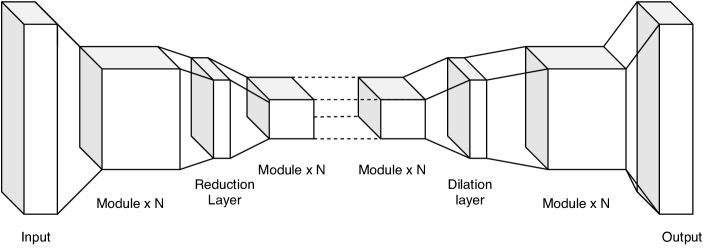
Figure 1: Diagram of modular autoencoder.

Autoencoders are a type of unsupervised learning technique consisting of two neural networks, an encoder network, denoted by $\psi_{e}$, and a decoder network, denoted by $\psi_{d}$, where the output of the encoder is fed into the decoder. The two networks are trained together such that the output of the decoder matches the input to the encoder. In other words, for an input $\mathbf{x}$:

$$\mathbf{\hat{x}}=\psi_{d}(\psi_{e}(\mathbf{x}))$$

and the goal is for the difference between $\mathbf{x}$ and $\mathbf{\hat{x}}$ to be as small as possible, as defined by the loss function. For a loss function $L$, the encoder and decoder (collectively referred to as the autoencoder) optimize the problem given by equation (1)

$$\Psi(\mathbf{x};\mathbf{\omega}_{e},\mathbf{\omega}_{d})=\min_{\mathbf{\omega}_{e},\mathbf{\omega}_{d}}L(\mathbf{x},\psi_{d}(\psi_{e}(\mathbf{x};\mathbf{\omega}_{e});\mathbf{\omega}_{d}))$$ (1)

where $\Psi(\mathbf{x};\mathbf{\omega})$ represents the encoder-decoder pair

$$\Psi(\mathbf{x};\mathbf{\omega})=(\psi_{e}(\mathbf{x};\mathbf{\omega}_{e}),\psi_{d}(\mathbf{x};\mathbf{\omega}_{d}))$$

and $\mathbf{\omega}_{e}$ and $\mathbf{\omega}_{d}$ are the weights of the encoder and decoder networks, respectively. Typically the encoder network is a mapping to a lower-dimensional space

$$\psi_{e}:\mathbb{R}^{d}\rightarrow\mathbb{R}^{d^{\prime}}$$

and the decoder network is a mapping from the lower-dimensional space to the original input space

$$\psi_{d}:\mathbb{R}^{d^{\prime}}\rightarrow\mathbb{R}^{d}$$

where $d^{\prime}\ll d$. The intuition behind this lower dimensional representation, or embedding, is that the autoencoder transforms the input into a representation that captures essential information and removes non-essential information. In practice, the size of this lower-dimensional representation, which we refer to as the intermediate representation, is a hyper-parameter of the autoencoder.

The autoencoders in this paper are constructed from repetitions of layer modules separated by reduction (dilation) modules, as shown in Figure 1. A module is an ordered collection of layers, separated by ReLU activations, as shown in Figure 2. Layer modules do not change the spatial dimensions of their input through the use of zero padding. Reducing the spatial dimensions of the input is left to the reduction module. Maintaining spatial dimension within layer modules allows us to guarantee properly formed networks during the neural network construction phase. A reduction module consists of a $1\times 1$ convolutional layer followed by a $2\times 2$ max pooling layer with stride two. The $1\times 1$ convolutional layer doubles the depth of the input layer’s filters, in an attempt to reduce the information loss resulting from the strided max pooling layer. The strided max pooling layer reduces each spatial dimension by a factor of two, resulting in an overall reduction in information of 75% (a quarter of the original spatial information is retained). Doubling the number of filters means the aggregate information loss is at least 50% rather than 75%. In the decoder network, reduction modules are replaced with dilation modules. The dilation modules replace the max pooling layer with a 2D convolutional transpose layer [20]. The effect of this layer is to expand the spatial dimension of its input.

Modular network designs, where the neural network is composed by repeating a layer module a set number of times, are a common technique in neural architecture search [8, 1, 9, 10, 11, 13, 14, 15]. It can also be seen in many popular network architectures such as Inception-v3 [21] and ResNets [22]. One of the primary advantages of using a modular network architecture is that we are able to reduce the size of the search space. For example, consider a modular network where the module has a maximum size of five layers and is repeated twice and there are two reduction layers. This network structure will result in a maximum network of 30 layers; however, because the search is performed at the module level, we only search the space of five layer networks. In our work we consider four different convolutional layers with four different filter counts as well as a 2D dropout layer; this gives 17 different options for each layer of the module. Using a modular network architecture enables us to reduce the search space from $\sim 10^{85}$ to $\sim 10^{15}$.

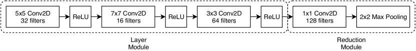
Figure 2: Example of a single layer module, followed by a reduction module.

3.1 Image Denoising

Image denoising solves the problem

$$\Psi=\min_{\mathbf{\omega}_{e},\mathbf{\omega}_{d}}L(\mathbf{X},\psi_{d}(\psi_{e}(\mathbf{X}+\mathbf{\epsilon};\mathbf{\omega}_{e});\mathbf{\omega}_{d}))$$ (2)

where the loss function, $L$, is typically the mean squared error (MSE) loss shown in equation 3. We choose MSE in this setting because it is a more appropriate choice for regression. If you consider the input and output of the autoencoder is two separate functions, the goal of training is to make them as similar as possible. While we could use binary cross entropy from a technical point of view, we find it is better suited to classification problems, of which autoencoders are decidedly not. On the other hand, one could extend our algorithm to include the loss function as a parameter of the search, as done by Rivera et al. [18].

$$L(\mathbf{X},\psi_{d}(\psi_{e}(\mathbf{X}+\lambda\epsilon)))=\sum_{\mathbf{x}\in\mathbf{X}}||\mathbf{x}-\psi_{d}(\psi_{e}(\mathbf{x}+\epsilon))||^{2}$$ (3)

and $\epsilon\sim N(0,\Sigma)$ where $\Sigma=\sigma^{2}\mathbb{I}$ and $\mathbb{I}$ is the identity matrix in $\mathbb{R}^{d\times d}$. We tune the difficulty of the denoising problem by modifying $\sigma$, larger $\sigma$ leads to noisier images. The intuition of denoising is rather simple, learn weights that allow the decoder to remove noise from a given image. There are a number of applications of this technique, the most obvious application being image restoration. However, initial work on denoising autoencoders actually used this technique as a method of pre-training the neural networks and then fine-tuning the encoder to be used in a classification task.

3.2 Manifold Learning

Manifold learning [4, 23, 5] is a form of non-linear dimensionality reduction. Manifold learning algorithms assume the data, $\mathbf{X}$, is sampled from a low-dimensional manifold $\mathcal{M}\subset\mathbb{R}^{d^{\prime}}$ embedded in a higher dimensional space $\mathbb{R}^{d}$, where $d^{\prime}\ll d$. Some of the more popular techniques are Isomap [24], locally-linear embeddings [25], and Laplacian eigenmaps [26]. Autoencoders are another technique for manifold learning. In this case, the encoder network $\psi_{e}$ is trained such that for input $\mathbf{X}\subset\mathbb{R}^{d}$

$$\psi_{e}:\mathbf{X}\subset\mathbb{R}^{d}\rightarrow\mathcal{M}$$

and the decoder network is trained such that it is a mapping

$$\psi_{d}:\mathcal{M}\rightarrow\mathbf{X}\subset\mathbb{R}^{d}$$

This technique is useful in high-dimensional settings as a feature selection technique, similar to Principal Component Analysis (PCA) [27] except that PCA is a linear dimensionality reduction technique and manifold learning is non-linear. A major difference between linear and non-linear manifold learning algorithms is that the linear algorithms attempt to preserve global structure in the embedded data while the non-linear algorithms only attempt to preserve local structure.

The primary challenge in manifold learning with autoencoders is two-fold: we must choose reasonably performant neural network architectures for the encoder and deocoder networks and we must also choose an appropriate dimension $d^{\prime}$. In this work we consider two $d^{\prime}$ values of $d^{\prime}=(1/4)d$ and $d^{\prime}=(1/8)d$, which we manually set for each experiment. The architecture of the networks is found via evolutionary search. In practice, we would chose $d^{\prime}$ as the smallest $d^{\prime}$ value that minimized the reconstruction loss $L(\mathbf{X},\psi_{d}(\psi_{e}(\mathbf{X})))$.

4 Evolving Deep Autoencoders

The two main approaches to neural architecture search are based on reinforcement learning or evolutionary algorithms. In this work we focus on the evolutionary approach, which consists of two primary components: evolution and selection. The evolution step is where new individuals (autoencoders in our case) are generated. The selection step is where the algorithm determines which individuals should survive and which individuals should be removed from the population. We use a generational selection mechanism where a population of network architectures goes through mutation, evaluation, and selection as a group. Specifically, we use $(\mu+\lambda)$ selection where a parent population of size $\mu$ generates $\lambda$ offspring and we select the top $\mu$ of the $\mu+\lambda$ individuals.

4.1 Network Construction

As discussed in Section 3, the autoencoders we consider in this paper consist of a layer module, followed by a reduction layer made up of a $1\times 1$ convolution and a $2\times 2$ max pooling layer—this structure may be optionally repeated, with each repetition reducing the dimension of the intermediate representation by 50%. We represent the module as a list of sequentially connected layer objects, encoded in a human-readable format. Each layer is defined by a layer token and a filter count, separated by a colon. Layers are separated by commas. For example, a module consisting of a $5\times 5$ convolution layer with 16 filters and two $3\times 3$ convolution layers with 32 filters would be represented:

5x5conv2d:16,3x3conv2d:32,3x3conv2d:32

This encoding is easy to work with in that it can be stored as a variable length array of strings, which allows us to handle layer mutation via indexing and addition of a layer by simply appending to the list. Of course, this could be condensed to a numerical coding scheme to reduce the size of the encoding. In our experience, using a more verbose encoding greatly simplified debugging and analyzing the results.

Using a sequential network architecture simplifies the construction process of the autoencoder when compared to a wide architecture such as the Inception module [21], where the module’s input can feed into multiple layers. Networks are constructed by assembling $1\times 1$, $2\times 2$, $3\times 3$, $5\times 4$, and $7\times 7$ 2D convolutional layers as well as a 2D dropout layer [28] with dropout probability $p=0.5$

We use convolutional layers, rather than dense layers, primarily because we use color image inputs in our experiments, which have three color channels for each pixel. Convolutional layers are useful for feature detection because they work on patches of pixels in the input. Additionally, they are an effective technique to reduce the total number of network parameters, resulting in smaller and faster training networks.

Our algorithm can work with any layer or activation function types and it would be appropriate to consider other layer types in different problem settings. For example, in a feature selection setting with dense data vectors it would make more sense to consider dense layers with evolving node counts rather than different types of convolutional layers.

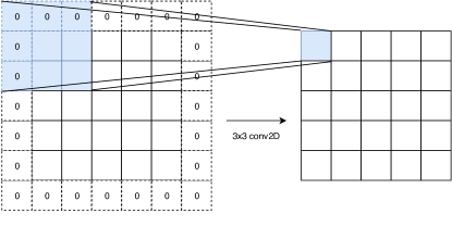
Figure 3: Illustration of a 2D $3\times 3$ convolutional layer with 0 padding to maintain the spatial dimensions of the input.

Figure 3 illustrates a $3\times 3$ convolutional layer with zero padding. We zero-pad all convolutional layers to maintain the spatial dimensions of the input, using the reduction(dilation) layers to modify spatial dimensions. Each layer can have 8, 16, 32, or 64 filters and the final output of the model is passed through a $\tanh$ activation function.

Algorithm 1 Evolutionary neural architecture search.

1:procedure EvolveNN($n,n_{\text{gen}}$)

2:     $P\leftarrow$ new population of size $n$

3:     for  $i=0$ to $n_{\text{gen}}$ do

4:         Mutate($P$)

5:         for  $p\in P$  do

6:              if $p$.isEvaluated then

7:                  continue

8:              else if  $p\in\texttt{cache.keys()}$ then

9:                  $p.\texttt{setFitness(cache.get(}p\texttt{))}$

10:              end if

11:              $t\leftarrow\texttt{Task}(p)$

12:              Send task $t$ to broker

13:         end for

14:         Wait for $|P|$ results from broker

15:         Update cache with received fitness values

16:         sort($P$)

17:         $P\leftarrow P[:n]$ $\triangleright$ Select top $n$ individuals

18:     end for

19:end procedure

Algorithm 2 Population evolution algorithm.

1:procedure Mutate($P$)

2:     $P^{\prime}\leftarrow P\texttt{.clone()}$

3:     for $p\in P$ do

4:         $o\leftarrow\texttt{RandomSample(}P\setminus p\texttt{)}$

5:         $u_{1}\leftarrow U(0,1)$

6:         $u_{2}\leftarrow U(0,1)$

7:         if $u_{1}<.5$ then

8:              $p\leftarrow\texttt{MutateGenotype(}p\texttt{)}$ $\triangleright$ Mutated clone of $p$

9:         end if

10:         if $u_{2}<.5$ then

11:              $o\leftarrow\texttt{MutateGenotype(}o\texttt{)}$ $\triangleright$ Mutated clone of $o$

12:         end if

13:         $c\leftarrow\texttt{Crossover(}p,o\texttt{)}$

14:         // Only add $p$ and $o$ to $P^{\prime}$ if they were mutated.

15:         $P^{\prime}\leftarrow P^{\prime}\cup\{p,o,c\}$

16:     end for

17:     return $P^{\prime}$

18:end procedure

Algorithm 3 Mutation and crossover algorithms used by the genotypes.

1:procedure MutateGenotype($g$)

2:     $c\leftarrow g\texttt{.clone()}$

3:     $z\leftarrow\texttt{SampleUniform(}0,1\texttt{)}$

4:     if $|c|<\texttt{MaxNumLayers}\textbf{and}z<0.5$ then

5:         $\texttt{AppendRandomLayer(}c\texttt{)}$

6:     else

7:         $\texttt{ReplaceRandomLayer(}c\texttt{)}$

8:     end if

9:     return c

10:end procedure

11:procedure Crossover($g_{1},g_{2}$)

12:     $i_{1}\leftarrow U(0,|g_{1}|$ $\triangleright$ Random layer index for $g_{1}$

13:     $i_{2}\leftarrow U(0,|g_{2}|$ $\triangleright$ Random layer index for $g_{2}$

14:     $c\leftarrow g_{1}\texttt{.layers}[:i_{1}]+g_{2}\texttt{.layers}[i_{2}:]$

15:     if $|c|>\texttt{MaxNumLayers}$ then

16:         //Drop layers exceeding size limit.

17:         $c\leftarrow c\texttt{.layers}[:\texttt{MaxNumLayers}]$

18:     end if

19:     return $c$

20:end procedure

The sequential approach also has a major advantage in that it is guaranteed to construct a valid network. Because each layer feeds into the next there will always be a path from input to output. This is not the case when allowing arbitrary connections between layers and letting evolution select these layers.

4.2 Network Evolution

Network architectures are evolved, as described by Algorithm 1, by starting with a minimal layer module (e.g., a single convolutional layer) and either mutating the module or by performing crossover with another layer module. The specific algorithm used to evolve the population a single generation is described in Algorithm 2 while Algorithm 3 describes the specific algorithms used to mutate individual genotypes and perform crossover between two genotypes. Mutation works by either appending a layer or modifying an existing layer. Crossover between two modules involves taking two network architectures and splicing them together. All of this is performed by the model, which is described in greater detail in Section 4.3. The autoencoder is packaged into a network task Protocol Buffer and sent to the Broker, which forwards them to a worker. The workers perform the task of training and evaluating the autoencoder, where evaluation is performed on validation data that the network as not previously seen. The validation loss is packaged in a result Protocol Buffer and sent back to the Broker, who then forwards the result to the model. We define fitness as the reciprocal of the validation loss, which has the nice property that low loss results in high fitness.

One notable aspect of our evolution algorithm is that we make it very likely one offspring is produced from each genotype in the parent population. We force crossover as long as the two selected genotypes have more than one layer each. This is similar to the forced mutation of Suganuma et al. [16]. The advantage is that we are constantly exploring new architectures; however, this approach also results in very large offspring populations that can be as large as $3\times$ the size of the parent population. If the parents were mutated during crossover their mutated selves are added into the original population. This differs from a more classical evolutionary algorithm in that mutation and crossover are strongly encouraged and forced. This adds variance to the overall population fitness, which we counter by using $(\mu+\lambda)$ selection, making sure we always maintain the best performing network architectures.

To cope with potentially large offspring population sizes, we make two modifications to the standard evolution algorithm to improve efficiency by reducing the total amount of work. These can be seen in lines 6 and 8 in Algorithm 1. In line 6, the model checks if the candidate autoencoder architecture (referred to as a genotype) has previously been evaluated. If the genotype was previously evaluated the model decides not to send it off for re-evaluation. This is possible because we make genotypes immutable—if a genotype is selected for mutation or crossover, a copy is made and mutated rather than modifying the original genotype. This modification alone can save anywhere from 25% (offspring population size $3\times$ that of the parent population) to 50% (offspring population size $2\times$ that of the parent population) because we use $(\mu+\lambda)$ selection, so the parent population is always included when evaluating the individuals of a population.

Similarly, in line 8, we check if the architecture of the genotype as been seen previously. Caching previously seen architectures and their respective fitness is particularly important because of the stochastic nature of the evolutionary search algorithm. We noticed during the experiments, especially at later generations of evolution when the population has started to homogenize, that previously encountered architectures would be rediscovered. This is expected because evolutionary search stochastically explores the neighborhood of the current position, which means it may explore previously seen locations (architectures) simply due to chance.

Let $\psi(\mathbf{x};\mathbf{\omega})$ represent a trained neural network with a fixed architecture. We denote training data as $\textbf{X}_{\text{tr}}$ and validation data as $\textbf{X}_{\text{val}}$. We define an autoencoder $\Psi=(\psi_{e},\psi_{d})$ as a tuple containing an encoder network, $\psi_{e}$, and a decoder network, $\psi_{d}$. Formally, the problem we solve in this work is shown in equation (4),

$$\Psi^{*}=\arg\min_{\psi\in\mathcal{A}}L(\textbf{X}_{\text{val}},\psi_{d}(\psi_{e}(X_{\text{val}})))$$ (4)

The optimal autoencoder for the given problem is given by $\Psi^{*}$, where optimality is defined with respect to an architecture in the space of all neural network architectures, $\mathcal{A}$. The loss function $L$ is mean-squared error, as defined in equation (5), where $\mathbf{X},\mathbf{Y}\in\mathbb{R}^{n\times d}$.

$$L(\mathbf{X},\mathbf{Y})=\frac{1}{n}\sum_{i=1}^{n}||\mathbf{x}-\mathbf{y}||^{2}$$ (5)

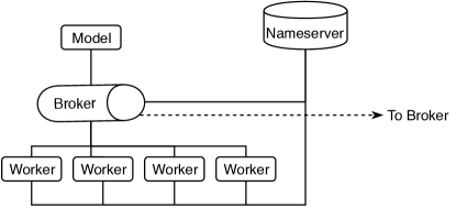
Figure 4: Overview of the system architecture.

4.3 System Architecture

We designed a system to efficiently find and evaluate deep autoencoders using the evolutionary algorithm described in Algorithm 1. We use the system proposed in [29] and shown in Figure 4, which consists of a model, one or more brokers, an arbitrary number of workers, and a nameserver. Flow of information through the system is rather simple – data flows from the model to the workers and then back to the model, all through the broker. Communication within the system is handled via remote procedure calls (RPC) using gRPC [30] and messages are serialized using Protocol Buffers [31]. The system infrastructure is written in Go while the model and worker implementations are written in Python and are availabe on GitHub. This is possible because of gRPC—we specify the system APIs in gRPC’s interface description language (IDL) and then implement them in Go and Python. The model and workers make use of the Python stubs and clients generated by gRPC from the API specification. The system moves the serialized Python objects from the model to the worker without having to worry about the contents of the messages. The advantage is that we can build the system infrastructure in a statically type-checked language such as Go while we can use Python and PyTorch [32] to build, train, and evaluate the autoencoder architectures. This is particularly important for the broker implementations; using Go gives the broker a high level of concurrency and performance when compared to Python.

Heartbeat messages are RPCs used by a client to inform a server that the client is still functioning. This is important when a client requests a resource within the system, such as a worker requesting a task from a broker. The resource may be lost if the client fails and no heartbeat mechanism is used. The heartbeat message informs the server if the client has failed, allowing the server to properly handle the shared resources.

Model

The model drives the evolutionary search for autoencoders by running the evolutionary algorithm that designs the layer modules. Once a population of layer modules has been generated (e.g., mutated or mated via crossover), the model packages the individual designs into tasks and sends them to the broker via RPC. The model then waits for the broker to send back the results from each of the layer module designs.

Broker

The broker forms the data pipeline of the system by moving data between the model and the workers. Unevaluated network architectures received from the model are stored in a queue. These network architectures–referred to as tasks–are removed from the queue and sent to a worker when a task request RPC is received from the respective worker. At this point the task is moved to a pending-completion state until the finished result is returned from the worker, at which point the result is forwarded to the model.

Brokers can connect (or link) with other brokers to share available compute resources. When connected with another broker, the broker stores shared tasks in a work queue, giving preference to its own tasks (referred to as owned tasks). Linked brokers are typically in different data centers because a single broker is capable of handling a large number of connected workers. Each network architecture evaluation takes on the order of minutes, giving the broker ample time to distribute tasks to other workers.

Worker

The worker is the computational engine of the system. Workers register with a broker when they request a task from the broker but are otherwise able to join or leave the system at-will. A worker begins a heartbeat RPC with the broker from which it requested a task. This heartbeat RPC ends once the task is complete and returned from the broker. In this sense, workers lease tasks from the broker. As a result, if a worker leaves the system after returning a task, no other components in the system will know the worker left and there will be no state within the system waiting for additional information from the worker.

Nameserver

The nameserver is a central store for the addresses of the brokers in the system. Models or workers can query the central store for a broker address prior to joining the system. This is not strictly required for the system, but improves the scalability of the system as more nodes are added. Rather than manually specifying the broker address for each worker, which may vary if there are many brokers, each worker can query the nameserver and get the address of a broker to connect to. Similarly, brokers can query the nameserver for the addresses of other brokers with whom they can form a link for work-sharing. As a result, the nameserver establishes a heartbeat with connected brokers. Brokers are removed from the nameserver’s list of available brokers when they fail to send a heartbeat within a specified time window. If the heartbeat is late, the nameserver will reply with a reconnect request to the broker, causing the broker to re-register with the nameserver.

Table 1: Fitness of top 3 found architectures for image denoising, trained for 20 epochs.

# of Epochs During Search	Rank	Architecture	Fitness
2	1	64-3x3conv2d	6.10
	2	64-7x7conv2d	5.97
	3	64-7x7conv2d - 64-3x3conv2d	5.86
5	1	64-5x5conv2d	6.02
	2	64-7x7conv2d	5.97
	3	64-7x7conv2d - 64-5x5conv2d	5.96
Random	-	-	$1.8\pm 1.52$

5 Experiments

We explore two areas of application in the experiments: manifold learning and image denoising. For all experiments we use the STL10 [33] dataset. We chose this dataset for its difficulty—the images are higher resolution than the CIFAR-10/100 [34] datasets, allowing more reduction modules. Additionally, the higher-resolution images are better suited for deeper, more complex autoencoder architectures.

The layer module is restricted to at most ten layers. This gives a sufficiently large search space of around 10 billion architectures. We also compare the found architectures against random search. Over-fitting is a challenge with deep autoencoders, so we restrict our models to only one layer module, rather than repeating the layer module multiple times. In our initial experiments we found autoencoders with multiple layer modules performed dramatically worse (due to over-fitting) than their single layer module counterparts.

The networks are implemented and trained using the PyTorch [32] framework. Evolutionary search is performed over 20 generations with a population size of 10 individuals. We use $(\mu+\lambda)$ selection as described in Algorithm 1.

Random Search

The random search comparisons are performed by sampling from $U[1,10]$, and using the sampled integer as the number of layers in the layer module. Each layer is determined by sampling a random layer type and a random number of filters. The number of layer modules and the number of reductions are hyper-parameters and set to the same values as the comparison architectures found via evolutionary search. We sample and evaluate 30 random architectures for each experiment.

Image Denoising

We used the image denoising experiments to test how well the evolutionary search algorithm performs when the candidate network architectures are trained for either two or five epochs. If the search can get away with fewer training epochs it will save resources, allowing the algorithm to explore more architectures. We set $\sigma^{2}=1/3$ in these experiments because we found that too much noise would cause the system to collapse and output blank images.

Manifold Learning

In the manifold learning setting we focus on a restricted set of reduced dimensions, namely those dimensions that are reduced by a factor of $(1/2)^{k}$ for $k=2$ and $3$. This greatly simplifies the construction of both the encoder and decoder networks. Each reduction module, consisting of a $1\times 1$ 2D convolutional layer followed by a stride 2, $2\times 2$ max pooling layer, reduces the each of the spatial dimensions by a factor of two. Thus the input dimension is reduced by 75% and 87.5%, respectively. This is a fairly drastic reduction in dimension and limits the total number of reduction modules used in a given autoencoder architecture.

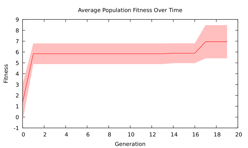
(a) Average fitness over 20 generations using two epochs during training.

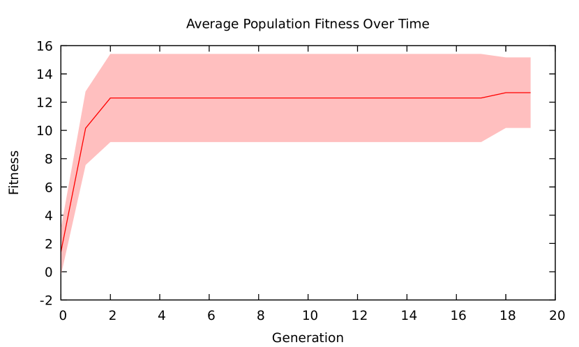
(b) Average fitness over 20 generations using five epochs during training.

Figure 5: Average fitness over 20 generations.

6 Discussion

We present the results form our experiments along with a discussion of their implications. All experiments were performed on Amazon Web Services (AWS) using Nvidia K80 GPUs. Fitness is defined as the reciprocal of the loss, lower loss leads to greater fitness. We train the final architectures for 20 epochs in the image denoising experiments and 40 epochs in the manifold learning experiments. In practice, this is a very small number of epochs for a production model; however, we kept this number low as it did not affect the results and reduced costs.

Random Search

Random search performed dramatically worse, on average, than evolutionary search on both the manifold learning and denoising tasks. This is unsurprising given the size of the search space, but differs from the claims of [19]. We train each random architecture for 20 epochs in the image denoising experiments and 40 epochs in the manifold learning experiments.

Image Denoising

Table 1 summarizes the results from the denoising experiments. We list the top three network architectures for the 2-epoch and 5-epoch searches, along with their fitness values after 20 epochs of training. Interestingly, both the 2-epoch and 5-epoch approaches found similar architectures and, perhaps more surprisingly, their third place architectures were combinations of the second and first place architectures.

It is unsurprising that both searches favored smaller architectures—the smaller epoch count means networks that train faster will have a better evaluation on the validation data. Smaller networks typically train faster than larger networks with respect to number of epochs, so it makes sense that these networks would rank higher during our searches using a limited number of epochs. On the other hand, over-fitting is an issue with the larger networks so favoring smaller layer module architectures had a positive impact on the overall performance of the autoencoder.

Figure 5 shows the average fitness across 20 generations for both the 2-epoch and 5-epoch searches. Both graphs share two similar features: they plateau at the second generation and maintain that plateau until around the 18th generation, when they both find better architectures. Although the 5-epoch graph has an unsurprisingly higher fitness, it is surprising that both approaches appear to improve at about the same pace. This reinforces the idea that the 2-epoch search does a decent job at exploring the space.

The un-noised input image is shown in Figure 6(a), the noised input images shown in Figure 6(b), and the denoised images shown in Figure 6(c).

(a) Original images (STL10 dataset).

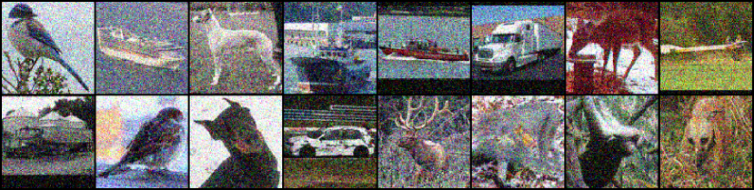
(b) Noised input images.

(c) Denoised output images (20 epochs of training).

Figure 6: Denoised images on unseen data.

Manifold Learning

Table 2: Fitness of top 3 found architectures for manifold learning, trained for 40 epochs.

# of Reduction Modules	Rank	Architecture	Fitness
2	1	64-5x5conv2d	9.05
	2	32-3x3conv2d	6.75
	3	32-7x7conv2d	4.99
	-	Random	$1.17\pm 1.22$
3	1	64-3x3conv2d	3.42
	2	64-5x5conv2d	3.38
	3	32-3x3conv2d - 64-5x5conv2d	2.4
	-	Random	$0.36\pm 0.30$

Figure 7: Scaling factors with respect to a single worker. These are calculated as the geometric average of the number of candidate architectures evaluated per generation, across five generations.

Table 3: Autoencoder architecture for Dropout example.

Image Effect	Layer Module Architecture
Greyscale	16-3x3conv2d – Dropout2D – 32-1x1conv2d – 2x2max-pool
Color	64-7x7conv2d – Dropout2D – 32-7x7conv2d – 2x2max-pool

Table 2 summarizes the results from performing evolutionary search on autoencoders using two and three reduction modules compared to random search. The search was performed over 20 generations, as is done in the denoising experiments. Because these networks are larger, we train them for 40 epochs instead of the 20 epochs used in the denoising experiments. Similar to the denoising experiments, random search performs worse than evolutionary search in all scenarios.

A single $5\times 5$ 2D convolutional layer as the layer module ranked highly in both the two and three reduction experiments at first and second place, respectively. As shown in Table 2, the 5x5conv2d layer with 64 filters performed nearly 50% better than the runner-up 3x3conv2d layer in the two reduction experiment. Interestingly, the 3x3conv2d and 5x5conv2d layers performed nearly identically in the three reduction experiment with the 3x3conv2d layer taking a slight lead. Perhaps more notably, the 5x5conv2d architecture performed nearly an order of magnitude better than random search in both experiments.

See the appendix for a demonstration of the results of the best autoencoder architectures found after 20 generations of search. Here we compare the resulting images of two and three reduction autoencoders. The reconstructed images using the two reduction autoencoder is shown in Figure 8(b) while the reconstructed images using the three reduction autoencoder is shown in Figure 8(c).

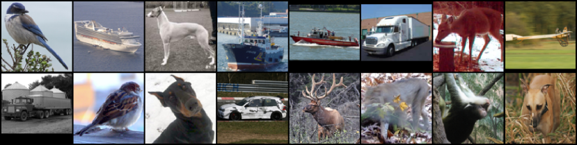
(a) Original input images (STL10 dataset).

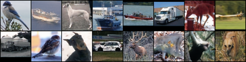
(b) Reconstructed image from autoencoder using two reduction layers. The original representation is reduced by 75%.

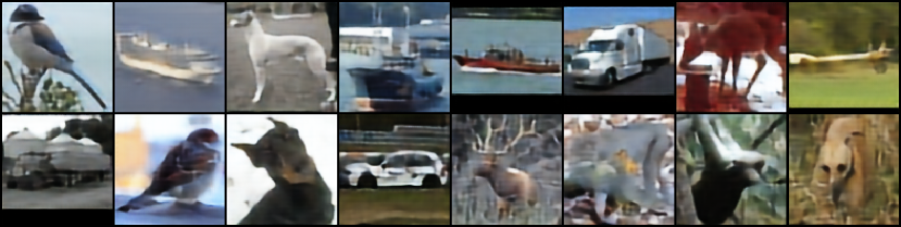
(c) Reconstructed image from autoencoder using three reduction layers. The original representation is reduced by 87.5%.

Figure 8: Comparison of best architectures found after 20 generations.

System Scalability

Figure 7 shows the scalability of the system. We were only able to test the system with a maximum of 16 nodes due to resource constraints. The system shows near linear scaling—the curve falls off from linear not due to scalability issues with the system architecture but due to node failures. We would occasionally experience GPU out-of-memory errors and this was more prevalent with larger node counts. Using an orchestration system such as Kubernetes [35] or Apache Mesos [36] would improve these scaling numbers as well as making the system more resilient.

Impact of Dropout Layers

Dropout layers have an interesting, if not somewhat unsurprising, effect on the output of the autoencoder. We give an example in the appendix of two different networks, whose architectures are described in Table 3, after 10 epochs of training. The output of the first network is greyscale while the output the second network is color (although it does exhibit some greyscale properties on some images). We use a 2D dropout layer [28] to regularize the autoencoders—during our experiments we noticed it was fairly easy to overfit the data so we decided to add a dropout layer to the list of potential layers used by the evolution algorithm. Note that, as described in [28], the 2D dropout layer drops out an entire channel at random during training. Despite both networks having a 2D dropout layer in the same position, the network that produces color output has a greater learning capacity due to its larger parameter count. In other words, this network has more filters (and thus more parameters) and uses these additional filters to store additional learned features of the dataset. This is what appears to the characteristic that allows the network to maintain coloring in the images. Somewhat surprisingly given the ease with which we noticed the autoencoders would overfit the data, none of the best architectures utilized a dropout layer.

(a) Input data (STL10 dataset)

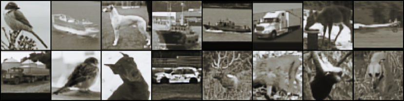
(b) Output from decoder after 10 epochs and three layer, layer module of 16-3x3conv2d – Dropout2D – 32-1x1conv2d, as described in Table 3.

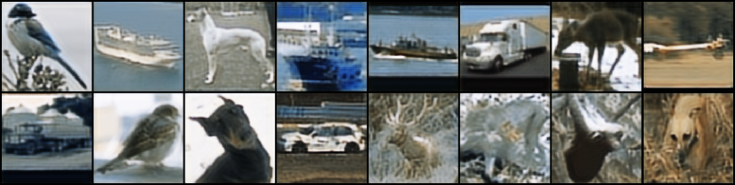
(c) Output from decoder after 10 epochs and three layer, layer module of 64-7x7conv2d – Dropout2D – 32-7x7conv2d, as described in Table 3.

Figure 9: Three layer module with a 2D dropout layer in the middle. Color information is preserved after 10 epochs of training.

7 Conclusion

We have introduced an efficient and scalable system for neural architecture search and demonstrated its effectiveness in designing deep autoencoders for image denoising and manifold learning. An interesting avenue for future work would be to extend the evolutionary algorithm based on the observations of the denoising experiments—rather than search a fixed space for all generations, use the first few generations to find smaller architectures that work well. After these architectures are found, reduce the search space to combinations of these architectures. This is similar, in a sense, to the work of [3]. Other important future work is improving individual worker efficiency, allowing the system to achieve similar performance using fewer workers. Although the large number of workers enables fast search of network architectures, each worker consumes valuable resource (e.g., monetary, compute, environmental, etc.). This work is important in enabling self-improving and automatic machine learning.

References

- [1] Barret Zoph and Quoc V. Le. Neural architecture search with reinforcement learning. 2017.
- [2] Esteban Real, Sherry Moore, Andrew Selle, Saurabh Saxena, Yutaka Leon Suematsu, Jie Tan, Quoc V. Le, and Alexey Kurakin. Large-scale evolution of image classifiers. In Doina Precup and Yee Whye Teh, editors, Proceedings of the 34th International Conference on Machine Learning, ICML 2017, Sydney, NSW, Australia, 6-11 August 2017, volume 70 of Proceedings of Machine Learning Research, pages 2902–2911. PMLR, 2017.
- [3] Hanxiao Liu, Karen Simonyan, Oriol Vinyals, Chrisantha Fernando, and Koray Kavukcuoglu. Hierarchical representations for efficient architecture search. CoRR, abs/1711.00436, 2017.
- [4] Yunqian Ma and Yun Fu. Manifold learning theory and applications. CRC press, 2011.
- [5] Ameet Talwalkar, Sanjiv Kumar, and Henry Rowley. Large-scale manifold learning. In 2008 IEEE Conference on Computer Vision and Pattern Recognition, pages 1–8. IEEE, 2008.
- [6] Pascal Vincent, Hugo Larochelle, Yoshua Bengio, and Pierre-Antoine Manzagol. Extracting and composing robust features with denoising autoencoders. In Proceedings of the 25th International Conference on Machine Learning, ICML ’08, pages 1096–1103, New York, NY, USA, 2008. ACM.
- [7] Pascal Vincent, Hugo Larochelle, Isabelle Lajoie, Yoshua Bengio, and Pierre-Antoine Manzagol. Stacked denoising autoencoders: Learning useful representations in a deep network with a local denoising criterion. J. Mach. Learn. Res., 11:3371–3408, 2010.
- [8] Hieu Pham, Melody Guan, Barret Zoph, Quoc Le, and Jeff Dean. Efficient neural architecture search via parameters sharing. In Jennifer Dy and Andreas Krause, editors, Proceedings of the 35th International Conference on Machine Learning, volume 80 of Proceedings of Machine Learning Research, pages 4095–4104, Stockholmsmässan, Stockholm Sweden, 7 2018. PMLR.
- [9] Hanxiao Liu, Karen Simonyan, and Yiming Yang. DARTS: differentiable architecture search. CoRR, abs/1806.09055, 2018.
- [10] David Ha, Andrew M. Dai, and Quoc V. Le. Hypernetworks. CoRR, abs/1609.09106, 2016.
- [11] Andrew Brock, Theodore Lim, James M. Ritchie, and Nick Weston. SMASH: one-shot model architecture search through hypernetworks. CoRR, abs/1708.05344, 2017.
- [12] George Kyriakides and Konstantinos G. Margaritis. Neural architecture search with synchronous advantage actor-critic methods and partial training. In Proceedings of the 10th Hellenic Conference on Artificial Intelligence, SETN ’18, pages 34:1–34:7, New York, NY, USA, 2018. ACM.
- [13] Jan Koutník, Giuseppe Cuccu, Jürgen Schmidhuber, and Faustino Gomez. Evolving large-scale neural networks for vision-based reinforcement learning. In Proceedings of the 15th Annual Conference on Genetic and Evolutionary Computation, GECCO ’13, pages 1061–1068, New York, NY, USA, 2013. ACM.
- [14] Risto Miikkulainen, Jason Zhi Liang, Elliot Meyerson, Aditya Rawal, Daniel Fink, Olivier Francon, Bala Raju, Hormoz Shahrzad, Arshak Navruzyan, Nigel Duffy, and Babak Hodjat. Evolving deep neural networks. CoRR, abs/1703.00548, 2017.
- [15] Chris Zhang, Mengye Ren, and Raquel Urtasun. Graph hypernetworks for neural architecture search. CoRR, abs/1810.05749, 2018.
- [16] Masanori Suganuma, Mete Ozay, and Takayuki Okatani. Exploiting the potential of standard convolutional autoencoders for image restoration by evolutionary search. In Jennifer Dy and Andreas Krause, editors, Proceedings of the 35th International Conference on Machine Learning, volume 80 of Proceedings of Machine Learning Research, pages 4771–4780, Stockholmsmässan, Stockholm Sweden, 7 2018. PMLR.
- [17] S. Lander and Y. Shang. Evoae – a new evolutionary method for training autoencoders for deep learning networks. In 2015 IEEE 39th Annual Computer Software and Applications Conference, volume 2, pages 790–795, 7 2015.
- [18] Francisco Charte, Antonio J Rivera, Francisco Martínez, and María J del Jesus. Automating autoencoder architecture configuration: An evolutionary approach. In International Work-Conference on the Interplay Between Natural and Artificial Computation, pages 339–349. Springer, 2019.
- [19] Christian Sciuto, Kaicheng Yu, Martin Jaggi, Claudiu Musat, and Mathieu Salzmann. Evaluating the search phase of neural architecture search. CoRR, abs/1902.08142, 2019.
- [20] Matthew D. Zeiler and Rob Fergus. Visualizing and understanding convolutional networks. In David Fleet, Tomas Pajdla, Bernt Schiele, and Tinne Tuytelaars, editors, Computer Vision – ECCV 2014, pages 818–833, Cham, 2014. Springer International Publishing.
- [21] Christian Szegedy, Vincent Vanhoucke, Sergey Ioffe, Jonathon Shlens, and Zbigniew Wojna. Rethinking the inception architecture for computer vision. CoRR, abs/1512.00567, 2015.
- [22] Kaiming He, Xiangyu Zhang, Shaoqing Ren, and Jian Sun. Deep residual learning for image recognition. In CVPR, pages 770–778. IEEE Computer Society, 2016.
- [23] Tong Lin and Hongbin Zha. Riemannian manifold learning. IEEE Transactions on Pattern Analysis and Machine Intelligence, 30(5):796–809, 2008.
- [24] Joshua B. Tenenbaum, Vin de Silva, and John C. Langford. A global geometric framework for nonlinear dimensionality reduction. Science, 290(5500):2319–2323, 2000.
- [25] Sam T. Roweis and Lawrence K. Saul. Nonlinear dimensionality reduction by locally linear embedding. SCIENCE, 290:2323–2326, 2000.
- [26] Mikhail Belkin and Partha Niyogi. Laplacian eigenmaps for dimensionality reduction and data representation. Neural Comput., 15(6):1373–1396, June 2003.
- [27] Hervé Abdi and Lynne J. Williams. Principal component analysis. WIREs Comput. Stat., 2(4):433–459, July 2010.
- [28] Jonathan Tompson, Ross Goroshin, Arjun Jain, Yann LeCun, and Christoph Bregler. Efficient object localization using convolutional networks. In IEEE Conference on Computer Vision and Pattern Recognition, CVPR 2015, Boston, MA, USA, June 7-12, 2015, pages 648–656. IEEE Computer Society, 2015.
- [29] Jeff Hajewski and Suely Oliveira. A scalable system for neural architecture search. In IEEE Computing and Communication Workshop and Conference, CCWC’20, 2020.
- [30] Google. grpc.
- [31] Kenton Varda. Protocol buffers: Google’s data interchange format. Technical report, Google, 6 2008.
- [32] Adam Paszke, Sam Gross, Soumith Chintala, Gregory Chanan, Edward Yang, Zachary DeVito, Zeming Lin, Alban Desmaison, Luca Antiga, and Adam Lerer. Automatic differentiation in PyTorch. In NIPS Autodiff Workshop, 2017.
- [33] Adam Coates, Andrew Y. Ng, and Honglak Lee. An analysis of single-layer networks in unsupervised feature learning. In Geoffrey J. Gordon, David B. Dunson, and Miroslav Dudík, editors, Proceedings of the Fourteenth International Conference on Artificial Intelligence and Statistics, AISTATS 2011, Fort Lauderdale, USA, April 11-13, 2011, volume 15 of JMLR Proceedings, pages 215–223. JMLR.org, 2011.
- [34] Alex Krizhevsky, Vinod Nair, and Geoffrey Hinton. Cifar-10 (canadian institute for advanced research).
- [35] David K. Rensin. Kubernetes - Scheduling the Future at Cloud Scale. 1005 Gravenstein Highway North Sebastopol, CA 95472, 2015.
- [36] Benjamin Hindman, Andy Konwinski, Matei Zaharia, Ali Ghodsi, Anthony D. Joseph, Randy Katz, Scott Shenker, and Ion Stoica. Mesos: A platform for fine-grained resource sharing in the data center. In Proceedings of the 8th USENIX Conference on Networked Systems Design and Implementation, NSDI’11, pages 295–308, Berkeley, CA, USA, 2011. USENIX Association.