The closest extremely low-mass white dwarf to the Sun

Abstract

We present the orbit and properties of 2MASS J050051.85–093054.9, establishing it as the closest ($d\approx 71$ pc) extremely low mass white dwarf to the Sun. We find that this star is hydrogen-rich with $T_{\textrm{eff}}\approx 10\,500$ K, $\log g\approx 5.9$, and, following evolutionary models, has a mass of $\approx 0.17$ $\mathrm{M}_{\mathrm{\sun}}$. Independent analysis of radial velocity and TESS photometric time series reveals an orbital period of $\approx$9.5 h. Its high velocity amplitude ($K\approx 144\leavevmode\nobreak\ \textrm{km}\,\textrm{s}^{-1}$) produces a measurable Doppler beaming effect in the TESS light curve with an amplitude of 1 mmag. The unseen companion is most likely a faint white dwarf. J0500$-$0930 belongs to a class of post-common envelope systems that will most likely merge through unstable mass transfer and in specific circumstances lead to Type Ia supernova explosions.

1 Introduction

With most stars ending their lives as white dwarfs (e.g., Fontaine et al., 2001), and most stars being in binaries (Moe & Di Stefano, 2017), there should be a large population of double-degenerate systems in our Galaxy. One interesting subset of these systems are extremely low mass (ELM) white dwarf (WD) binaries, where one of the stars has a mass $\leq$0.3 $\mathrm{M}_{\mathrm{\sun}}$. Such a low mass cannot be achieved through canonical single-star evolution (e.g., Marsh, 1995), so these ELM WDs must undergo significant mass loss during their evolution. Observationally, they are relatively rare objects ($\sim$100 are known; Brown et al., 2020), and with only a few exceptions (Brown et al., 2016a), they have been found to be in short-period (hours to minutes) binaries.

Beyond their interest for stellar evolution, these compact binary systems are predicted to emit gravitational waves. The magnitude of the strain measured by detectors like the future LISA instrument (Amaro-Seoane et al., 2012) depend on the inverse of the distance (as well as the inclination of the system) so that the identification and characterization of the nearest systems is important.

In this work we present a detailed analysis of 2MASS J05005185$-$0930549 (hereafter J0500$-$0930) which confirms a suggestion offered by Scholz et al. (2018), later seconded by Pelisoli & Vos (2019), that J0500$-$0930 is an ELM WD with an effective temperature $T_{\rm eff}\approx 11,900\pm 1100\leavevmode\nobreak\ {\rm K}$ and a surface gravity $\log g\leq 6.5$.The measured Gaia DR2 parallax of $\varpi=13.97\pm 0.05$ mas places it at a distance of $71.41\pm 0.27$ pc (Bailer-Jones et al., 2018) making it the closest known ELM WD. Its low mass and close proximity mean that it is also one of the brightest (in an apparent sense) known ELM WDs. We demonstrate that J0500$-$0930 is part of a short-period, post-interacting double degenerate system with an unseen WD companion.

2 Observations

In this section we describe the original discovery observations and follow-up spectroscopic observations (Section 2.1) and survey photometric data (Section 2.2).

2.1 Spectroscopic observations

J0500$-$0930 was serendipitously observed by the GALAH survey (De Silva et al., 2015; Martell et al., 2017; Buder et al., 2018) on 2017 January 5 using the 3.9-metre Anglo-Australian Telescope with the HERMES spectrograph (Sheinis et al., 2015) and the Two-Degree Field fibre positioner top-end (Lewis et al., 2002). The GALAH survey is a large spectroscopic investigation of the local stellar environment and its simple, magnitude-limited selection function includes stars such as J0500$-$0930 that fall outside of its normal aim of targeting unevolved disk stars. HERMES provides $\sim$1000 Å of non-contiguous wavelength coverage at a spectral resolving power of $R\approx 28\,000$. The raw spectra for the field containing J0500$-$0930 were reduced using the 2dfdr pipeline (v6.46 AAO Software Team, 2015) using the standard HERMES configuration.

As a follow-up, J0500$-$0930 was observed on the nights of 2019 November 5, 2019 December 16–20, and 2020 January 24–29 with the WiFeS integral field spectrograph (Dopita et al., 2010) on the ANU 2.3-m telescope at Siding Spring Observatory. The instrumental setup employed the R3000/B3000 red/blue grating combination in 2019 November and the R7000/B3000 combination in subsequent runs at a nominal resolution specified by the grating label. The setup delivered a wavelength coverage of 3500–5900Å in the blue and 5300–7000Å (R7000) or 5300–9600Å (R3000) in the red. The spectra were extracted, sky-subtracted, and wavelength calibrated using arc lamp exposures taken after stellar exposures to compensate for small wavelength shifts. The spectra were reduced using FIGARO (Shortridge, 1993). The reduced spectra were then (relative) flux-calibrated using observations of a number of known flux standards obtained each night. A total of 36 individual exposures were acquired with WiFeS.

2.2 Photometric observations

The Transiting Exoplanet Survey Satellite (TESS; Ricker et al., 2014) is obtaining 27 d time series photometry in a sequence of sectors that will cover over 85 per cent of the sky. J0500$-$0930 (TIC ID 43529091: Stassun et al., 2019) is located in Sector 5 (observed 2018 November 15 to December 11) of the TESS southern sky monitoring mission. It was not a target of interest, so we have only the 30 min cadence Full Frame Images. We used the eleanor software package (Feinstein et al., 2019) to download and background-subtract a $13\times 13$ pixel Target Pixel File centred on J0500$-$0930. We required high quality observations ($\texttt{quality}==0$), and only used cadences with dates $\mathrm{BJD}-2458438=0.78$–12.20 and 13.60–25.64 to eliminate Earthshine contamination. This provided 1080 valid observations and 52 rejections.

Table 1 lists photometric measurements from GALEX (Morrissey et al., 2007), SkyMapper DR2 (Onken et al., 2019), 2MASS (Skrutskie et al., 2006) and WISE (Cutri & et al., 2012). The $NUV$ magnitude was corrected ($\Delta NUV=-0.073$) for detector non-linearity (Morrissey et al., 2007).

Table 1: Identification and measurements of J0500$-$0930.

Parameter		Measurement			Ref.
RA (2000)		05h00m51$\aas@@fstack{s}$85			1
Dec (2000)		-09°30′54$\aas@@fstack{\prime\prime}$9			1
GALAH ID		170105002601114			2
Gaia DR2 ID		3183166667278838656			3
Parallax		$13.975\pm 0.052$ mas			3
$\mu_{\alpha}\cos{\delta}$		$-48.551\pm 0.074$ mas yr-1			3
$\mu_{\delta}$		$-121.871\pm 0.073$ mas yr-1			3
Period (Light curve)		$9.458\pm 0.011$ hr			4
Period (RV curve)		$9.462506\pm 0.000017$ hr			4
Photometry
Band	Measurement	Ref.	Band	Measurement	Ref.
$FUV$	$14.287\pm 0.009$	5	$u$	$13.347\pm 0.007$	8
$NUV$	$14.122\pm 0.008$	5	$v$	$13.016\pm 0.005$	8
$J$	$12.649\pm 0.026$	6	$g$	$12.514\pm 0.007$	8
$H$	$12.707\pm 0.030$	6	$r$	$12.699\pm 0.007$	8
$K$	$12.709\pm 0.030$	6	$i$	$12.982\pm 0.005$	8
$W1$	$12.628\pm 0.024$	7	$z$	$13.202\pm 0.005$	8
$W2$	$12.689\pm 0.027$	7

References: (1) Skrutskie et al. (2006); (2) Buder et al. (2018); (3) Gaia Collaboration et al. (2018); (4) This work; (5) Morrissey et al. (2007); (6) Skrutskie et al. (2006); (7) Cutri & et al. (2012); (8) Onken et al. (2019).

3 Analysis

We proceed with a determination of the stellar parameters (Section 3.1) of the primary component of J0500$-$0930 and the parameters of the orbit (Section 3.2). Additional insights on this system are gained through an analysis of the TESS light curve (Section 3.3).

The spectroscopic time series enables an analysis of the orbital parameters as well as the stellar parameters of the primary star. We found no spectroscopic signatures that would belong to the secondary star which we refer to as the unseen companion.

3.1 Atmospheric and stellar parameters

We derived the physical properties of J0500$-$0930 using a combination of spectroscopic, photometric and astrometric data. We employed a grid of hydrogen-rich model atmospheres allowing for traces of heavier elements (He, C, N, O, Si, Ca, Fe). The models allow for convective and radiative energy transport. Model convergence is achieved with conservation of the total flux ($F_{\rm convective}+F_{\rm radiative}$) within 0.1 per cent error. The same models were used in the analysis of the ELM NLTT 11748 (Kawka & Vennes, 2009) but with updated Balmer line profiles as described in Kawka & Vennes (2012).

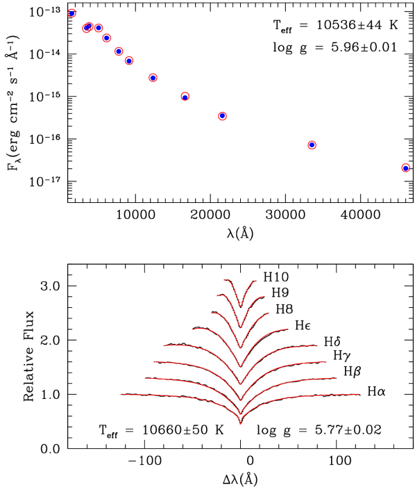
Figure 1: Top panel: The observed spectral energy distribution (blue points) compared to the best fitting magnitudes (open red circles). Bottom panel: Representative Balmer line spectrum (black) compared to the corresponding best fitting model spectrum (red).

First, we fitted the Balmer line profiles from H$\alpha$ to H₁₀ varying $T_{\textrm{eff}}$ and $\log g$. The line profiles are shaped by the temperature and density structure of the atmosphere and are dominated by Stark broadening. The upper Balmer lines are also affected by pressure ionization effects which are modelled using an energy level dilution scheme (Hummer & Mihalas, 1988) with details provided by Kawka & Vennes (2006). Fig 1 shows a representative result of the line profile fitting procedure with the corresponding best fit parameters. A set of 36 ($T_{\textrm{eff}}$, $\log g$) measurements was obtained from the WiFeS spectra from which we computed the weighed average and dispersion:

$$T_{\textrm{eff}}=10\,650\pm 110\ {\rm K},\ \log g=5.76\pm 0.05\ \ \ \ \ \ {\rm(Balmer)}.$$

The measurements do not correlate with the orbital phase with a Pearson correlation coefficient smaller than $\approx 0.2$. Next, we constrained $\log g$ using the Gaia DR2 distance measurement, $d_{\rm Gaia}$. The surface gravity is measured indirectly using mass-radius relations (Serenelli et al., 2001; Istrate et al., 2016) and a constraint on the stellar radius $R$ set by the observed absolute magnitude $M_{\rm obs}=m-(5\log d_{\rm Gaia}-5)$ for a given photometric band. Synthetic absolute magnitudes, $M_{\rm mod}\,(T_{\textrm{eff}},\log g$), are obtained by folding the model spectra with appropriate bandpasses. Equating $M_{\rm mod}=M_{\rm obs}$, we solve numerically for $\log g$ at a given $T_{\textrm{eff}}$. Therefore, the observed Balmer spectra are fitted as a function of $T_{\textrm{eff}}$ with $\log g$ constrained by the Gaia parallax. In the present analysis with adopted the SkyMapper $g$ band. The weighed average and dispersion of the set of 36 ($T_{\textrm{eff}}$, $\log g$) measurements are:

$$T_{\textrm{eff}}=10\,390\pm 60\ {\rm K},\ \log g=5.93\pm 0.01\ \ \ \ {\rm(Balmer-\textit{Gaia})}.$$

Finally, we fitted the spectral energy distribution (SED) mapped by a set of photometric measurements, $m_{i}$ (Table 1). Again, the apparent magnitudes are converted into absolute magnitudes, $M_{{\rm obs},i}$, and fitted to the set of synthetic absolute magnitudes (computed as above), $M_{{mod},i}$, as a function of $T_{\textrm{eff}}$. The best fitting parameters are:

$$T_{\textrm{eff}}=10\,536\pm 44\ {\rm K},\ \log g=5.96\pm 0.01\ \ \ \ {\rm(SED-\textit{Gaia})}.$$

The SED does not show evidence of the secondary star, which is most likely a fainter WD. The solutions constrained by the Gaia distance measurement are marginally consistent, but show systematic differences with $\log g$ measurements obtained fitting the Balmer line profiles alone. All solutions are model dependent: the Gaia parallax measurement constrains the stellar radius, and, indirectly $\log g$ by applying mass/radius relations; model Balmer line profiles that constrain $\log g$ depend on pressure broadening and energy level prescriptions.

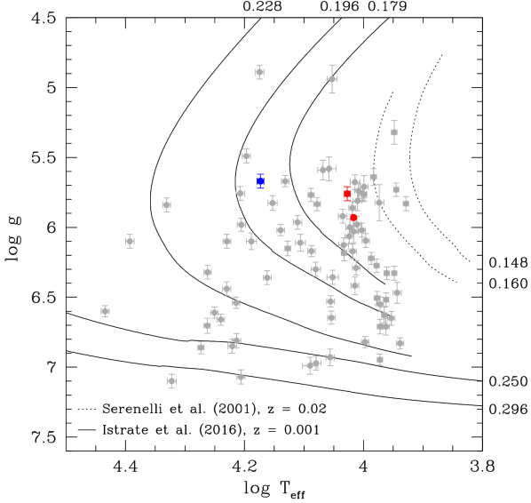
Figure 2: Effective temperature and surface gravity measurements of known ELM WDs are shown with grey symbols. J0500$-$0930 (Balmer line profile fits with and without Gaia) and GALEX J1717+6757 are shown with red and blue circles, respectively. The ELM WDs are compared to cooling tracks (see text) labelled with the mass ($\mathrm{M}_{\mathrm{\sun}}$).

A close examination of the blue spectrum of J0500$-$0930 does not show evidence of the Ca ii H&K doublet. Adopting stellar parameters obtained with the joint SED-Gaia data set and varying the calcium abundance we measured an abundance (by number) upper limit (99 per cent) of $\log\,{\rm Ca/H}\lesssim-10.7$. The calcium abundance upper-limit indicates that J0500$-$0930 does not belong to the group of high-metallicity ELM WDs described by Gianninas et al. (2014). Using evolutionary tracks for ELM WDs from Serenelli et al. (2001) and Istrate et al. (2016) and combining the ($T_{\textrm{eff}}$,$\log g$) measurements described above we calculate a mass of $0.17\pm 0.01$ $\mathrm{M}_{\mathrm{\sun}}$. Fig. 2 compares 2MASS J0500-0930 to other known ELM WDs (Brown et al., 2020; Vennes et al., 2011) and to the cooling tracks of Serenelli et al. (2001) and Istrate et al. (2016). The stellar parameters place J0500$-$0930 amongst the lowest-mass WDs.

3.2 Period analysis

We measured the radial velocity of the ELM WD in HERMES and WiFeS spectra by fitting a Gaussian function to the deep, narrow Doppler core ($\pm 2$Å) of H$\alpha$. The mid-exposure HJD times and corresponding radial velocities in the heliocentric rest frame are provided in the Supplementary Material. We fitted the data with a sinusoidal function

$$v(t)=\gamma+K\,sin[2\pi(t-T_{0})/P]$$

where $P$ is the orbital period, $T_{0}$ is the epoch of inferior conjunction for the ELM, $\gamma$ is the systemic velocity and $K$ is the ELM semi-amplitude velocity. Individual error bars were set at approximately one tenth of a resolution element corresponding to the rms of the fitting procedure, which dominates the error budget, and providing increased weight to higher resolution spectra. Fig. 3 shows the results of the analysis that delivered $P$ and $T_{0}$:

$$P=0.3942711\pm 0.0000007\ {\rm d}\ (=9.462506\pm 0.000017\ {\rm h}),$$

$$T_{0}\,({\rm HJD})=2458318.0472\pm 0.0004.$$

The ELM motion is described by $K=143.7\pm 0.9\leavevmode\nobreak\ \textrm{km}\,\textrm{s}^{-1}$ and $\gamma=-45.0\pm 1.2\leavevmode\nobreak\ \textrm{km}\,\textrm{s}^{-1}$. Velocity residuals averaged 5 $\textrm{km}\,\textrm{s}^{-1}$ which validates the velocity error bars.

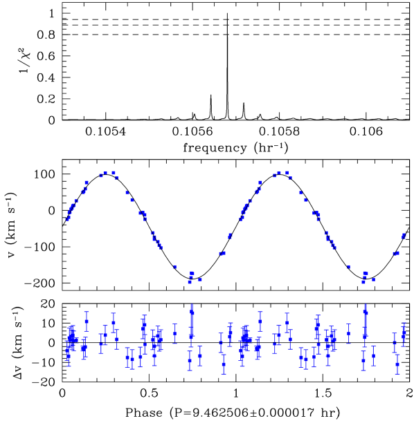
Figure 3: Period analysis of radial velocity measurements. The top panel shows $\chi^{2}$ function as a function of the frequency in cycles per hour. The horizontal dashed lines represent confidence levels at 66 (top), 90 and 99 per cent (bottom). The middle panel shows the radial velocity measurements (squares) folded on the orbital period and best fitting sine curve, and the bottom panel shows the radial velocity residuals.

3.3 TESS Light curve

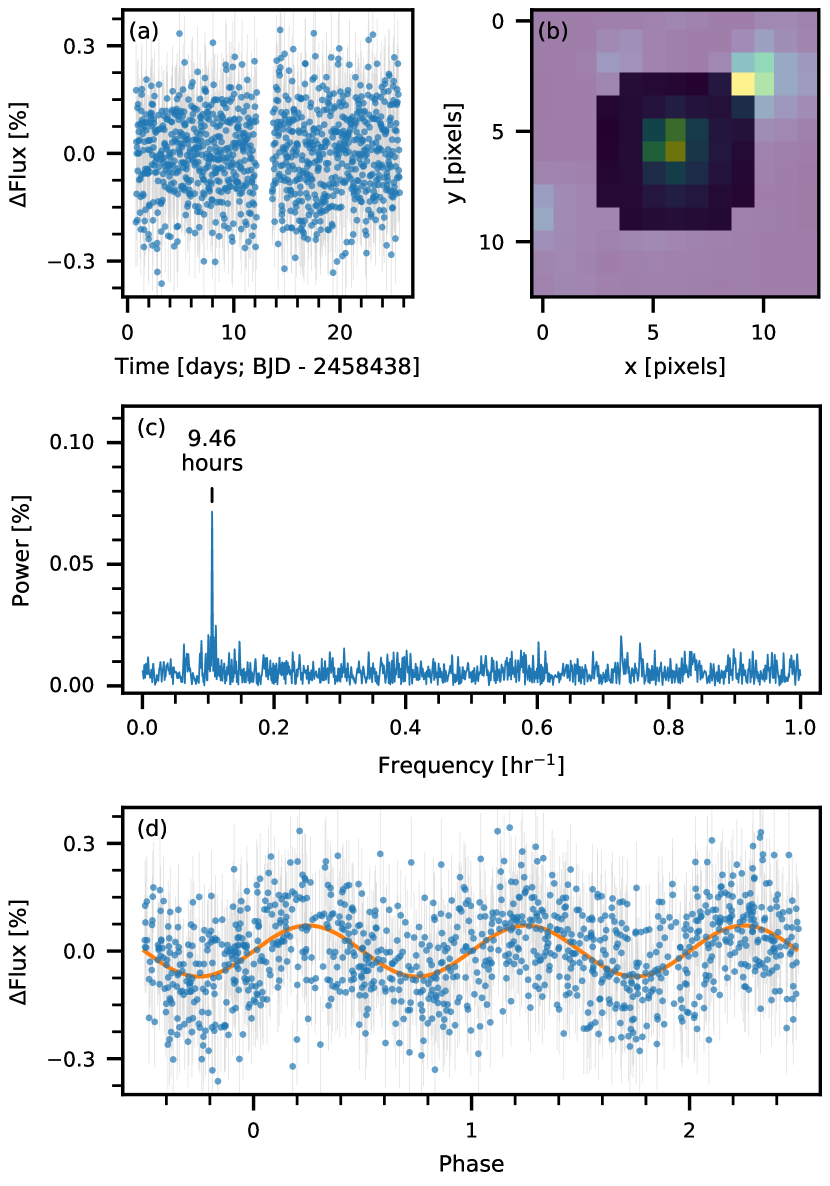
Figure 4: (a) the light curve measured by eleanor. (b) a 13-by-13 pixel cutout of a TESS full frame image, with the aperture used by eleanor indicated as the darker region. (c) the periodogram of the light curve, with the period of the peak frequency indicated (9.46 h) (d) the light curve folded on a period of 9.458 h, showing a sinusoidal behaviour. The orange curve is a sine function with a period of 9.458 h and amplitude of 0.070 per cent.

ELM WDs have been found to show evidence for eclipses, Doppler beaming, ellipsoidal, and reflection effects in their light curves (Faigler & Mazeh, 2011). A light curve from the TESS photometry was constructed with eleanor with a PCA-based detrending of the raw aperture photometry and modelling the PSF of the star at each cadence to generate a light curve. A normalized light curve was found with flux errors of $\approx$0.22 per cent (Fig. 4). The periodogram was built using lightkurve (v1.6.0; Lightkurve Collaboration et al., 2018, 2019) and the default Lomb-Scargle method (Lomb, 1976; Scargle, 1982; Press & Rybicki, 1989) implemented using astropy (The Astropy Collaboration et al., 2018). This showed one clear peak at $\sim$9.46 h with an amplitude of $\sim$0.071 per cent — very similar to the orbital period found from the RV observations.

To quantify the uncertainties of these values, we used emcee to fit a sinusoidal model to the light curve. This found an amplitude of $0.070\pm 0.010$ per cent, a period of $9.458\pm 0.011$ h, and a $T_{0}\,{\rm(BJD)}=2458438.114\pm 0.017$. The light curve does not show any evidence for eclipses deeper than 0.03 per cent at the observed 30 min cadence. At an inclination of 90$\degr$, an eclipse depth of 5 per cent with a duration of $\approx 3$ min, or 0.5 per cent at a 30 min cadence, would have been observed assuming radii of 0.077 and 0.017 $\mathrm{R}_{\mathrm{\sun}}$ for the ELM and a cooler, 0.3 $\mathrm{M}_{\mathrm{\sun}}$ WD companion, respectively. Shorter, shallower eclipses remain detectable at inclinations $\gtrsim 87$°.

The period of the light curve is in agreement with the orbital period. When phasing the light curve on the orbital period it shows evidence for the Doppler beaming effect which is caused by light concentration in the direction of motion. We observed the flux maximum at an epoch corresponding to orbital phase $\Phi_{\rm orb}=0.78\pm 0.04$ in agreement with the predicted $\Phi_{\rm orb}=0.75$ (Fig. 3). Since the ELM WD outshines its higher mass WD companion, the amplitude of the beaming effect can be estimated using $A\approx\alpha e^{\alpha}/(e^{\alpha}-1)\times(K/c)$ (van Kerkwijk et al., 2010), where $c$ is the speed of light, $K$ is the velocity semi-amplitude, and $\alpha=h\nu/kT_{\rm eff}$, where $\nu$ is the frequency of the photometric bandpass. In the TESS bandpass we expect an $\approx$1 mmag amplitude for the beaming effect compared to an observed amplitude of $0.77$ mmag. The concurrence of the predicted and observed phases and amplitudes affirms the Doppler beaming effect as the explanation for the variability.

4 Discussion and Summary

With a mass function of 0.12 $\mathrm{M}_{\mathrm{\sun}}$, the minimum companion mass at an inclination $i=90^{\circ}$ is 0.3 $\mathrm{M}_{\mathrm{\sun}}$, assuming an ELM mass of 0.17 $\mathrm{M}_{\mathrm{\sun}}$ (see Section 3.1). Conversely, if the companion is a normal 0.6 $\mathrm{M}_{\mathrm{\sun}}$ WD, the inclination would be $\approx$45°.

With the systemic radial velocity of the system calculated (see Section 3.2), we now have the 6D space information, from which we calculate its Galactic orbit properties. As in Simpson et al. (2017) the orbit was calculated using galpy with the default options and with the Milky Way potential defined by MWPotential2014. We find that J0500$-$0930 is on a disk-like orbit, with peri-orbit of $r_{\mathrm{perio}}=6.73\pm 0.01$ kpc, apo-orbit $r_{\mathrm{apo}}=11.61\pm 0.09$ kpc, an eccentricity of $e=0.27\pm 0.01$, and a maximum distance above the plane of $z_{\mathrm{max}}=0.02\pm 0.01$ kpc. About two-thirds of ELM are found in the disk (Brown et al., 2020).

Future gravitational wave detectors will have the ability to detect some double-generate systems with $P<1$ hr. Although J0500$-$0930 is not in this regime, we decided to calculate the characteristic strain, as this value is dependent on the inverse of the distance. Using equation 2 from Brown et al. (2020), and assuming a fixed mass of the ELM of 0.17 $\mathrm{M}_{\mathrm{\sun}}$, for the reasonable range of secondary masses ($0.3<M_{2}<0.6$ $\mathrm{M}_{\mathrm{\sun}}$), the gravitational wave strain ($h_{c}$) for a four-year LISA mission will be in the range of $0.5\times 10^{-20}<h_{c}<2.0\times 10^{-20}$. This unfortunately is several orders of magnitude below the detection limit.

It will take a few tens of Gyrs for 2MASS J0500-0930 to merge through the loss of gravitational radiation (Ritter, 1986). More specifically the ELM WD would merge with a companion of a mass of 0.6 $\mathrm{M}_{\mathrm{\sun}}$ in 36 Gyr. Brown et al. (2020) show that most ELM WD binaries will merge through unstable mass transfer (Shen, 2015) rather than become AM CVn binaries.

The GALAH survey will cover up to approximately half of the sky at a limiting magnitude of $V_{\rm lim}=14$ (De Silva et al., 2015), hence it probed so far a volume $\lesssim 0.5\,(4\pi/3)\,d_{\rm max}^{3}$, where $\log\,d_{\rm max}=(V_{\rm lim}-M_{V}+5)/5$. With an absolute magnitude $M_{V}\approx 8.2$, J0500$-$0930 adds a dominant contribution ($\gtrsim 160$ kpc^-3) to the local space density of ELM WDs which is comparable to the density estimated by Brown et al. (2016b).

In summary, we have confirmed J0500$-$0930 as the closest ELM WD to the Sun at a distance of 71 pc, while the next one was found at 178 pc (GALEX J1717+6757, Vennes et al., 2011). The minimum companion mass of 0.3 $\mathrm{M}_{\mathrm{\sun}}$ and the lack of infrared excess indicate that the companion is a fainter WD with a higher mass and lower effective temperature. The TESS light curve does not show evidence of an eclipse and is modulated over the orbital period by the Doppler beaming effect. Its kinematics show that J0500$-$0930 belongs to the disk population. Finally, J0500$-$0930 will merge with its companion in a time $>t_{\rm Hubble}$ with the likelihood of a Type Ia supernova event dependent on the secondary mass.

References

- AAO Software Team (2015) AAO Software Team 2015, 2dfdr: Data Reduction Software
- Amaro-Seoane et al. (2012) Amaro-Seoane P., et al., 2012, Classical and Quantum Gravity, 29, 124016
- Bailer-Jones et al. (2018) Bailer-Jones C. A. L., Rybizki J., Fouesneau M., Mantelet G., Andrae R., 2018, AJ, 156, 58
- Bovy (2015) Bovy J., 2015, ApJS, 216, 29
- Brown et al. (2016a) Brown W. R., Gianninas A., Kilic M., Kenyon S. J., Prieto C. A., 2016a, ApJ, 818, 155
- Brown et al. (2016b) Brown W. R., Kilic M., Kenyon S. J., Gianninas A., 2016b, ApJ, 824, 46
- Brown et al. (2020) Brown W. R., et al., 2020, ApJ, 889, 49
- Buder et al. (2018) Buder S., et al., 2018, MNRAS, 478, 4513
- Caswell et al. (2020) Caswell T. A., et al., 2020, Matplotlib/Matplotlib v3.1.3
- Cutri & et al. (2012) Cutri R. M., et al. 2012, VizieR Online Data Catalog, p. II/311
- De Silva et al. (2015) De Silva G. M., et al., 2015, MNRAS, 449, 2604
- Dopita et al. (2010) Dopita M., et al., 2010, Ap&SS, 327, 245
- Faigler & Mazeh (2011) Faigler S., Mazeh T., 2011, MNRAS, 415, 3921
- Feinstein et al. (2019) Feinstein A. D., et al., 2019, PASP, 131, 094502
- Fontaine et al. (2001) Fontaine G., Brassard P., Bergeron P., 2001, PASP, 113, 409
- Foreman-Mackey et al. (2013a) Foreman-Mackey D., et al., 2013a, ASCL, p. ascl:1303.002
- Foreman-Mackey et al. (2013b) Foreman-Mackey D., Hogg D. W., Lang D., Goodman J., 2013b, PASP, 125, 306
- Gaia Collaboration et al. (2018) Gaia Collaboration et al., 2018, A&A, 616, A1
- Gianninas et al. (2014) Gianninas A., Dufour P., Kilic M., Brown W. R., Bergeron P., Hermes J. J., 2014, ApJ, 794, 35
- Hummer & Mihalas (1988) Hummer D. G., Mihalas D., 1988, ApJ, 331, 794
- Hunter (2007) Hunter J. D., 2007, Computing in Science & Engineering, 9, 90
- Istrate et al. (2016) Istrate A. G., Marchant P., Tauris T. M., Langer N., Stancliffe R. J., Grassitelli L., 2016, A&A, 595, A35
- Kawka & Vennes (2006) Kawka A., Vennes S., 2006, ApJ, 643, 402
- Kawka & Vennes (2009) Kawka A., Vennes S., 2009, A&A, 506, L25
- Kawka & Vennes (2012) Kawka A., Vennes S., 2012, A&A, 538, A13
- Lewis et al. (2002) Lewis I. J., et al., 2002, MNRAS, 333, 279
- Lightkurve Collaboration et al. (2018) Lightkurve Collaboration et al., 2018, ASCL, p. ascl:1812.013
- Lightkurve Collaboration et al. (2019) Lightkurve Collaboration et al., 2019, KeplerGO/Lightkurve: Lightkurve v1.6.0, doi:10.5281/zenodo.3579358
- Lomb (1976) Lomb N. R., 1976, Astrophysics and Space Science, 39, 447
- Marsh (1995) Marsh T. R., 1995, MNRAS, 275, L1
- Martell et al. (2017) Martell S. L., et al., 2017, MNRAS, 465, 3203
- Moe & Di Stefano (2017) Moe M., Di Stefano R., 2017, ApJS, 230, 15
- Morrissey et al. (2007) Morrissey P., et al., 2007, ApJS, 173, 682
- Onken et al. (2019) Onken C. A., et al., 2019, Publ. Astron. Soc. Australia, 36, e033
- Pelisoli & Vos (2019) Pelisoli I., Vos J., 2019, MNRAS, 488, 2892
- Press & Rybicki (1989) Press W. H., Rybicki G. B., 1989, ApJ, 338, 277
- Ricker et al. (2014) Ricker G. R., et al., 2014, Journal of Astronomical Telescopes, Instruments, and Systems, 1, 014003
- Ritter (1986) Ritter H., 1986, A&A, 169, 139
- Scargle (1982) Scargle J. D., 1982, ApJ, 263, 835
- Scholz et al. (2018) Scholz R.-D., Meusinger H., Schwope A., Jahreiß H., Pelisoli I., 2018, A&A, 619, A31
- SciPy 1.0 Contributors et al. (2020) SciPy 1.0 Contributors et al., 2020, Nature Methods
- Serenelli et al. (2001) Serenelli A. M., Althaus L. G., Rohrmann R. D., Benvenuto O. G., 2001, MNRAS, 325, 607
- Sheinis et al. (2015) Sheinis A., et al., 2015, J. Astron. Telesc. Instruments, Syst., 1, 35002
- Shen (2015) Shen K. J., 2015, ApJ, 805, L6
- Shortridge (1993) Shortridge K., 1993, in Hanisch R. J., Brissenden R. J. V., Barnes J., eds, ASP Conf. Ser. Vol. 52, Astronomical Data Analysis Software and Systems II. ASP, p. 219
- Simpson et al. (2017) Simpson J. D., De Silva G., Martell S. L., Navin C. A., Zucker D. B., 2017, MNRAS, 472, 2856
- Skrutskie et al. (2006) Skrutskie M. F., et al., 2006, AJ, 131, 1163
- Stassun et al. (2019) Stassun K. G., et al., 2019, AJ, 158, 138
- The Astropy Collaboration et al. (2018) The Astropy Collaboration et al., 2018, AJ, 156, 123
- Vennes et al. (2011) Vennes S., et al., 2011, ApJ, 737, L16
- van Kerkwijk et al. (2010) van Kerkwijk M. H., Rappaport S. A., Breton R. P., Justham S., Podsiadlowski P., Han Z., 2010, ApJ, 715, 51