Multi-boundary correlators in JT gravity

Abstract

We continue the systematic study of the thermal partition function of Jackiw-Teitelboim (JT) gravity started in [arXiv:1911.01659]. We generalize our analysis to the case of multi-boundary correlators with the help of the boundary creation operator. We clarify how the Korteweg-de Vries constraints arise in the presence of multiple boundaries, deriving differential equations obeyed by the correlators. The differential equations allow us to compute the genus expansion of the correlators up to any order without ambiguity. We also formulate a systematic method of calculating the WKB expansion of the Baker-Akhiezer function and the ’t Hooft expansion of the multi-boundary correlators. This new formalism is much more efficient than our previous method based on the topological recursion. We further investigate the low temperature expansion of the two-boundary correlator. We formulate a method of computing it up to any order and also find a universal form of the two-boundary correlator in terms of the error function. Using this result we are able to write down the analytic form of the spectral form factor in JT gravity and show how the ramp and plateau behavior comes about. We also study the Hartle-Hawking state in the free boson/fermion representation of the tau-function and discuss how it should be related to the multi-boundary correlators.

1 Introduction

Jackiw-Teitelboim (JT) gravity Jackiw:1984je ; Teitelboim:1983ux is a very useful toy model to study various issues in quantum gravity and holography. As discussed in Almheiri:2014cka ; Maldacena:2016upp ; Jensen:2016pah ; Engelsoy:2016xyb , JT gravity is holographically dual to the low energy Schwarzian sector of the Sachdev-Ye-Kitaev (SYK) model Sachdev ; kitaev2015simple . In a recent paper Saad:2019lba Saad, Shenker and Stanford showed that the partition function of JT gravity on asymptotically Euclidean AdS spacetime is equal to the partition function of a certain double-scaled random matrix model and the contributions of higher genus spacetimes originated from the splitting and joining of baby universes is captured by the $1/N$ expansion of the matrix model. See also Stanford:2019vob ; Blommaert:2019wfy ; Okuyama:2019xbv ; Johnson:2019eik ; Kapec:2019ecr ; Betzios:2020nry for related works in this direction. This opens up an interesting avenue to study the effect of topology change in holography using the powerful techniques of the random matrix theory. This connection between JT gravity and the random matrix model comes from the fact that the density of states in Schwarzian theory is exactly equal to the planar (genus-zero) eigenvalue density of the random matrix model which arises in the topological recursion of the Weil-Petersson volume Eynard:2007kz . This connection is very interesting from the viewpoint of holography. It clearly shows that JT gravity is dual to an ensemble of boundary theories and the partition function on asymptotic AdS spacetime with renormalized boundary length $\beta$ is interpreted as the ensemble average $\langle Z(\beta)\rangle=\langle\operatorname{Tr}e^{-\beta H}\rangle$ over the random Hamiltonian $H$.

In our previous paper Okuyama:2019xbv , we showed that JT gravity is nothing but a special case of the Witten-Kontsevich topological gravity Witten:1990hr ; Kontsevich:1992ti and we studied the partition function $\langle Z(\beta)\rangle$ of JT gravity on spacetime with a single asymptotic boundary in detail. In particular, we found that $\langle Z(\beta)\rangle$ is written as the expectation value of the macroscopic loop operator in 2d gravity Banks:1989df . The important difference of JT gravity from the known example of 2d gravity is that infinitely many couplings $t_{k}$ are turned on with a specific value $t_{k}=\gamma_{k}$ with

$$\gamma_{0}=\gamma_{1}=0,\quad\gamma_{k}=\frac{(-1)^{k}}{(k-1)!}~{}~{}~{}(k\geq 2).$$ (1)

By generalizing the approach of Zograf Zograf:2008wbe , we found that the contributions of the higher genus topologies can be systematically computed by making use of the KdV constraint obeyed by the partition function. As emphasized in Zograf:2008wbe , this method serves as a very fast algorithm for the higher genus computation compared to the Mirzakhani’s recursion relation for the Weil-Petersson volume mirzakhani2007simple . We also found that in the low temperature regime the genus expansion can be reorganized in the following scaling limit, which we call the ’t Hooft limit

$$\hbar\to 0,~{}\beta\to\infty\quad\text{with}\quad\lambda=\hbar\beta~{}~{}~{}\text{fixed},$$ (2)

where $\hbar\sim e^{-S_{0}}$ is the genus-counting parameter. In this limit the free energy $\log\langle Z(\beta)\rangle$ admits the ’t Hooft expansion

$$\log\langle Z(\beta)\rangle=\sum_{k=0}^{\infty}\hbar^{k-1}\mathcal{F}_{k}(\lambda)$$ (3)

and we found the analytic form of the first few terms of $\mathcal{F}_{k}(\lambda)$.

We emphasize that this ’t Hooft limit is not just taking the low temperature limit and replacing the Schwarzian density of states $\rho(E)\sim\sinh(2\sqrt{E})$ by the Airy one $\rho(E)\sim\sqrt{E}$. Even after taking the ’t Hooft limit, we still keep all the non-trivial information of the spectral curve $y=\frac{1}{2}\sin(2\sqrt{x})$ of JT gravity matrix model. In particular, the leading term $\mathcal{F}_{0}(\lambda)$ in (3) is given by an integral on the spectral curve $y=\frac{1}{2}\sin(2\sqrt{x})$

$$\mathcal{F}_{0}(\lambda)=2\int_{0}^{\lambda/2}xdy=\int_{0}^{\lambda/2}\frac{1}{2}\arcsin(2y)^{2}dy.$$ (4)

The Airy case corresponds to the cubic polynomial $\mathcal{F}_{0}(\lambda)_{\text{Airy}}=\frac{\lambda^{3}}{12}$ and we start to see the deviation from the Airy case at the order $\mathcal{O}(\lambda^{5})$. One might worry that by taking the ’t Hooft limit we throw away all the interesting part of the black hole physics coming from the high energy states. However, as we will see in section 5, we indeed observe the Hawking-Page like transition between the disconnected Euclidean black holes and the connected Euclidean wormhole within the leading approximation of the ’t Hooft expansion. This clearly shows that our ’t Hooft expansion captures the interesting part of the physics of black holes. Another concern is that there are only order one number of states left above the ground state after taking the ’t Hooft limit and the naive gravity description breaks down. However, JT gravity is dual to an averaged system with continuous density of states from the beginning and it is not sensitive enough to distinguish black hole microstates. Moreover, in the low temperature limit $\beta\to\infty$ the boundary has a macroscopic length in units of the Planck length and hence there is no problem in describing such a situation by a smooth geometry. See also Iliesiu:2020qvm for a recent discussion of the absence of mass gap in the spectrum of the near-extremal charged black hole in 4d, whose near horizon dynamics is described by JT gravity.

In the present paper, we will study the partition function of JT gravity on spacetimes with multiple boundaries by generalizing the method of KdV equation in Okuyama:2019xbv . We find that the KdV constraints for the connected part of the multi-boundary correlator $\langle\prod_{i}Z(\beta_{i})\rangle_{\mbox{\scriptsize c}}$ is obtained by acting the “boundary creation operators” $B(\beta_{i})$ to the original KdV equation for the potential $u(x)$. Our boundary creation operator $B(\beta)$ is the same as the one discussed in the old 2d gravity literature Moore:1991ir ; Ginsparg:1993is which is based on the idea that the macroscopic loop operator is expanded in terms of the microscopic loop operators in the limit $\beta\to 0$, up to the so-called non-universal terms which scale with negative powers of $\beta$. We can systematically compute the genus expansion of the correlator $\langle\prod_{i}Z(\beta_{i})\rangle_{\mbox{\scriptsize c}}$ by solving this KdV constraints recursively. Most of the computation can be done away from the “on-shell” value of the couplings (1). In particular, we define the off-shell generalization of the effective potential and its Legendre transform, the off-shell free energy. We find that the multi-boundary correlators can be written in terms of a certain combination of the off-shell free energy in the ’t Hooft limit. We also study the WKB expansion of the Baker-Akhiezer (BA) functions.

In this paper we will focus on the two-point function and compute its genus expansion using the above formalism. We also compute its low temperature expansion and study its behavior in the ’t Hooft limit as well. It turns out that the two-point function in JT gravity is expressed in terms of the error function, which is a natural generalization of the known result of pure topological gravity okounkov2002generating . From the bulk gravity viewpoint, the connected part of the two-point function $\langle Z(\beta_{1})Z(\beta_{2})\rangle_{\mbox{\scriptsize c}}$ corresponds to a Euclidean wormhole (also known as the “double trumpet” Saad:2018bqo ) connecting the two asymptotically AdS boundaries with renormalized lengths $\beta_{1},\beta_{2}$. The analytic continuation of the two-point function $\langle Z(\beta+\mathrm{i}t)Z(\beta-\mathrm{i}t)\rangle_{\mbox{\scriptsize c}}$, known as the spectral form factor (SFF), is of particular interest in the context of quantum chaos and the SFF is widely studied in the SYK model and JT gravity Garcia-Garcia:2016mno ; Cotler:2016fpe ; Saad:2018bqo ; Saad:2019pqd . We find the analytic form of the SFF in the ’t Hooft limit and show that the SFF in JT gravity exhibits the characteristic feature of the so-called ramp and plateau, as expected for a chaotic system with random matrix statistics of eigenvalues.

In a recent interesting paper Marolf:2020xie , Marolf and Maxfield considered the boundary creation operators in the context of the AdS/CFT correspondence and made some interesting argument on the baby universe Hilbert space building upon the earlier works by Coleman Coleman:1988cy and by Giddings and Strominger Giddings:1988cx ; Giddings:1988wv . The argument in Marolf:2020xie is mostly based on the intuition coming from a simple toy model, which is not a full-fledged JT gravity. It is interesting to ask how our boundary creation operator $B(\beta)$ fits into the story in Marolf:2020xie , but we do not have a clear understanding of it. We make some preliminary remarks on this problem in section 6 and leave the details for a future work.

This paper is organized as follows. In section 2, we compute the genus expansion of multi-boundary correlators using the KdV constraint obeyed by these correlators. In section 3, we consider the WKB expansion of the Baker-Akhiezer functions and the ’t Hooft expansion of the multi-boundary correlators. Along the way, we define the off-shell extension of the effective potential and the free energy. In section 4, we compute the low temperature expansion of the two-boundary correlator. In section 5, we study the spectral form factor in JT gravity and show that it exhibits the ramp and plateau behavior as expected for chaotic system. In section 6, we consider the free boson/fermion representation of the $\tau$-function and discuss the boundary creation operator in this formalism. Finally we conclude in section 7. In appendix A, we consider the wavefunction of microscopic loop operators in the ’t Hooft limit.

2 Genus expansion

2.1 Basics and conventions

In this paper we will generalize our method Okuyama:2019xbv developed for one-boundary partition function to the case of multi-boundary correlators. To begin with, let us summarize basics, notations and conventions.

As we showed in Okuyama:2019xbv , JT gravity can be regarded as a special case of the general Witten-Kontsevich topological gravity Witten:1990hr ; Kontsevich:1992ti . In this model the intersection numbers

$$\langle\kappa^{\ell}\tau_{d_{1}}\cdots\tau_{d_{n}}\rangle_{g,n}=\int_{\overline{\cal M}_{g,n}}\kappa^{\ell}\psi_{1}^{d_{1}}\cdots\psi_{n}^{d_{n}},\qquad\ell,d_{1},\ldots,d_{n}\in{\mathbb{Z}}_{\geq 0}$$ (5)

play the role of correlation functions. They are defined on a closed Riemann surface $\Sigma$ of genus $g$ with $n$ marked points $p_{1},\ldots,p_{n}$. We let ${\cal M}_{g,n}$ denote the moduli space of $\Sigma$ and $\overline{\cal M}_{g,n}$ the Deligne-Mumford compactification of ${\cal M}_{g,n}$. $\kappa$ (often denoted as $\kappa_{1}$ in the literature) is the first Miller-Morita-Mumford class, which is proportional to the Weil-Petersson symplectic form $\omega=2\pi^{2}\kappa$. $\psi_{i}$ is the first Chern class of the complex line bundle whose fiber is the cotangent space to $p_{i}$ and $\tau_{d_{i}}=\psi_{i}^{d_{i}}$. The intersection number in (5) obeys the selection rule

$$\int_{\overline{\cal M}_{g,n}}\kappa^{\ell}\psi_{1}^{d_{1}}\cdots\psi_{n}^{d_{n}}=0\quad\mbox{unless}\quad\ell+d_{1}+\cdots+d_{n}=3g-3+n,$$ (6)

which we will use frequently.

For the above correlation functions one can introduce the generating functions

$$\begin{aligned} G(s,\{t_{k}\})&:=\sum_{g=0}^{\infty}g_{\rm s}^{2g-2}G_{g}(s,\{t_{k}\}),&F(\{t_{k}\})&:=\sum_{g=0}^{\infty}g_{\rm s}^{2g-2}F_{g}(\{t_{k}\}),\\ G_{g}(s,\{t_{k}\})&:=\left\langle e^{s\kappa+\sum_{d=0}^{\infty}t_{d}\tau_{d}}\right\rangle_{g},&F_{g}(\{t_{k}\})&:=\left\langle e^{\sum_{d=0}^{\infty}t_{d}\tau_{d}}\right\rangle_{g}.\end{aligned}$$ (7)

$G$ is actually expressed in terms of $F$ as Mulase:2006baa ; Dijkgraaf:2018vnm

$$G(s,\{t_{k}\})=F(\{t_{k}+\gamma_{k}s^{k-1}\}),$$ (8)

where $\gamma_{k}$ is defined in (1). Using this property we showed Okuyama:2019xbv that JT gravity is nothing but the special case of the general Witten-Kontsevich gravity with $t_{k}=\gamma_{k}$. Conversely, we can define a natural deformation of JT gravity by (partially) releasing $t_{k}$ from the constraint $t_{k}=\gamma_{k}$ and regard them as deformation parameters. This is one of our main ideas in Okuyama:2019xbv and enables us to investigate JT gravity using the techniques of the traditional 2d gravity. In what follows we will apply this prescription to multi-boundary correlators.

In this paper we study the $n$-boundary connected correlator of JT gravity

$$\langle Z(\beta_{1})\cdots Z(\beta_{n})\rangle_{\mbox{\scriptsize c}}.$$ (9)

We consider two kinds of its generalizations, $Z_{n}(\beta_{1},\ldots,\beta_{n};t_{0},t_{1})$ and $Z_{n}(\beta_{1},\ldots,\beta_{n};\{t_{k}\})$. They are obtained respectively by releasing only $t_{0},t_{1}$ or all $\{t_{k}\}$ from the constraint $t_{k}=\gamma_{k}$. We often call them “off-shell” correlators. They are related to the “on-shell” correlators (9) as

$$\begin{aligned} Z_{n}(\beta_{1},\ldots,\beta_{n},t_{0},t_{1},\{t_{k}=\gamma_{k}\}_{k\geq 2})&=Z_{n}(\beta_{1},\ldots,\beta_{n},t_{0},t_{1}),\\ Z_{n}(\beta_{1},\ldots,\beta_{n},t_{0}=0,t_{1}=0)&=\langle Z(\beta_{1})\cdots Z(\beta_{n})\rangle_{\mbox{\scriptsize c}}.\end{aligned}$$ (10)

As in Okuyama:2019xbv we introduce the notations

$$\hbar:=\frac{1}{\sqrt{2}}g_{\rm s},\quad x:=\hbar^{-1}t_{0},\quad\tau:=\hbar^{-1}t_{1}$$ (11)

and

$$\partial_{k}:=\frac{\partial}{\partial t_{k}},\quad{}^{{}^{\prime}}:=\partial_{x}=\hbar\partial_{0},\quad\dot{~{}}:=\partial_{\tau}=\hbar\partial_{1}.$$ (12)

As discussed in Okuyama:2019xbv , $g_{\rm s}$ is the genus-counting parameter in the high temperature regime while $\hbar$ is the natural coupling constant in the low temperature ’t Hooft limit (2). It is also convenient to introduce

$$I_{n}(v,\{t_{k}\})=\sum_{\ell=0}^{\infty}t_{n+\ell}\frac{v^{\ell}}{\ell!}\quad(n\geq 0),$$ (13)

because it is known Itzykson:1992ya that $F_{g}(\{t_{k}\})\ (g\geq 2)$ are polynomials in $I_{n}(u_{0},\{t_{k}\})\ (n\geq 2)$ and in $[1-I_{1}(u_{0},\{t_{k}\})]^{-1}$, with

$$u_{0} :=\partial_{0}^{2}F_{0}.$$ (14)

We will work mostly on the partially constrained case $t_{k}=\gamma_{k}\ (k\geq 2)$, leaving $t_{0}$ and $t_{1}$ as parameters. In this case we further introduce the new variables

$$y:=u_{0},\quad t:=1-I_{1}$$ (15)

and the functions

$$B_{n}(y):=\frac{J_{n}(2\sqrt{y})}{y^{n/2}}=\sum_{k=\max(0,-n)}^{\infty}\frac{(-1)^{k}y^{k}}{k!(k+n)!}\qquad(n\in{\mathbb{Z}}).$$ (16)

Here, $J_{n}(z)$ is the Bessel function of the first kind. $B_{n}$ are related to $I_{n}$ as

$$B_{n-1} =(-1)^{n}I_{n}(y,\{t_{0},t_{1},t_{k}=\gamma_{k}\ (k\geq 2)\})\quad(n\geq 2)$$ (17)

and satisfy

$$\partial_{y}B_{n} =-B_{n+1},\qquad yB_{n+1}=nB_{n}-B_{n-1}.$$ (18)

The old variables $(t_{0},t_{1})$ and the new ones $(y,t)$ are related as

$$t_{1}=B_{0}-t,\quad t_{0}=y(B_{1}-t_{1}).$$ (19)

The differentials $\partial_{0,1}$ are then written in the new variables as

$$\partial_{0}=\frac{1}{t}(\partial_{y}-B_{1}\partial_{t}),\quad\partial_{1}=y\partial_{0}-\partial_{t}.$$ (20)

The on-shell value $(t_{0},t_{1})=(0,0)$ corresponds to $(y,t)=(0,1)$. At this value $B_{n}$ becomes

$$B_{n}(0)=\frac{1}{n!},\quad n\geq 0.$$ (21)

2.2 Multi-boundary correlators of general topological gravity

In our previous paper Okuyama:2019xbv we formulated how to compute the genus expansion of the partition function $Z_{1}=Z_{\mbox{\scriptsize JT}}$ of JT gravity on a surface with one boundary. In this section we generalize the method to the case of multi-boundary correlators of general topological gravity.

Let us start with the fact that the $n$-boundary correlator of general topological gravity is given by Moore:1991ir

$$\begin{aligned} Z_{n}(\{\beta_{i}\},\{t_{k}\})&\simeq B(\beta_{1})\cdots B(\beta_{n})F(\{t_{k}\}).\end{aligned}$$ (22)

Here $F$ is defined in (7) and the operator $B(\beta)$ is given by

$$B(\beta)=g_{\rm s}\sqrt{\frac{\beta}{2\pi}}\sum_{d=0}^{\infty}\beta^{d}\partial_{d}.$$ (23)

As mentioned in section 1, (23) is based on the idea that the macroscopic loop operator $Z(\beta)$ is expanded in terms of the microscopic loop operator $\tau_{d}$ in the limit $\beta\to 0$

$$Z(\beta)\simeq g_{\rm s}\sqrt{\frac{\beta}{2\pi}}\sum_{d=0}^{\infty}\beta^{d}\tau_{d}$$ (24)

and the insertion of $\tau_{d}$ is represented by the derivative $\partial_{d}$ when acting on the free energy $F$. $B(\beta)$ can be thought of as the “boundary creation operator.” We put the symbol “$\simeq$” in (22), meaning that the equality holds up to an additional non-universal part Moore:1991ir when $3g-3+n<0$. Such a deviation appears, however, only in the genus-zero part of $n=1,2$-boundary correlators, which we will discuss separately in section 2.3. Note that the complex dimension of the moduli space $\overline{\mathcal{M}}_{g,n}$ is $3g-3+n$ which becomes negative for $(g,n)=(0,1)$ and $(0,2)$.

As in the case of single boundary the genus expansion can be computed by solving a differential equation which follows from the KdV equation. To see this, let us first introduce

$$\begin{aligned} W_{n}(\{\beta_{i}\},\{t_{k}\}):=&\ \partial_{x}Z_{n}=\hbar\partial_{0}Z_{n}\\ \simeq&\ \hbar B(\beta_{1})\cdots B(\beta_{n})\partial_{0}F,\\ W_{0}(\{t_{k}\}):=&\ \partial_{x}F=\hbar\partial_{0}F,\\ u:=&\ g_{\rm s}^{2}\partial_{0}^{2}F=2\partial_{x}^{2}F.\end{aligned}$$ (25)

Recall that $u$ satisfies the KdV equation Witten:1990hr ; Kontsevich:1992ti

$$\dot{u}=uu^{\prime}+\frac{1}{6}u^{\prime\prime\prime}.$$ (26)

Integrating this equation once in $x=\hbar^{-1}t_{0}$ we have

$$\dot{W}_{0} =(W_{0}^{\prime})^{2}+\frac{1}{6}W_{0}^{\prime\prime\prime}.$$ (27)

Since $B(\beta_{i})$ commutes with $\dot{~{}}=\partial_{\tau}$ and ${}^{\prime}=\partial_{x}$, we immediately obtain a differential equation for $W_{n}$ by simply acting $B(\beta_{1})\cdots B(\beta_{n})$ on both sides of the above equation. For instance, by acting $B(\beta_{1})$ on both sides of (27) we obtain

$$\begin{aligned} \dot{W}_{1}&=2W_{0}^{\prime}W_{1}^{\prime}+\frac{1}{6}W_{1}^{\prime\prime\prime}\\ &=uW_{1}^{\prime}+\frac{1}{6}W_{1}^{\prime\prime\prime}\end{aligned}$$ (28)

for $W_{1}(\beta_{1})$. This is nothing but the differential equation for $W$ in Okuyama:2019xbv with the identification $W_{1}=W$. By further acting $B(\beta_{2})$ on both sides of (28) we obtain

$$\begin{aligned} \dot{W}_{2}(\beta_{1},\beta_{2})&=2W_{1}^{\prime}(\beta_{1})W_{1}^{\prime}(\beta_{2})+2W_{0}^{\prime}W_{2}^{\prime}(\beta_{1},\beta_{2})+\frac{1}{6}W_{2}^{\prime\prime\prime}(\beta_{1},\beta_{2})\\ &=2W_{1}^{\prime}(\beta_{1})W_{1}^{\prime}(\beta_{2})+uW_{2}^{\prime}(\beta_{1},\beta_{2})+\frac{1}{6}W_{2}^{\prime\prime\prime}(\beta_{1},\beta_{2}).\end{aligned}$$ (29)

In general the differential equation for $W_{n}$ may be written as

$$\begin{aligned} \dot{W}_{n}(\beta_{1},\ldots,\beta_{n})&=\sum_{I\subset N}W_{|I|}^{\prime}W_{|N-I|}^{\prime}+\frac{1}{6}W_{n}^{\prime\prime\prime}(\beta_{1},\ldots,\beta_{n}),\end{aligned}$$ (30)

where $N=\{1,2,\ldots,n\}$, $W_{|I|}^{\prime}=W_{|I|}^{\prime}(\beta_{i_{1}},\ldots,\beta_{i_{|I|}})$ with $I=\{i_{1},i_{2},\ldots,i_{|I|}\}$ and the sum is taken for all possible subset $I$ of $N$ including the empty set. The equation (30) uniquely determines $W_{n}$ in the genus expansion given the genus expansion of $W_{k}\ (k<n)$ and the genus zero part $W_{n}^{g=0}$. It is important to note that the non-universal parts are entirely absent in (30) because all the elements other than $W_{0}^{\prime}=\frac{u}{2}$ appearing in (30) are equal to or higher than the third derivative of $F_{0}$ (see the discussion in the next subsection).

Finally $Z_{n}$ is obtained by merely integrating $W_{n}$ once in $x$. This can be done order by order in the genus expansion. As a demonstration we will study in detail the case of two-boundary correlator of JT gravity in subsection 2.4.

2.3 Genus zero part

In this section let us consider the genus zero part of the multi-boundary correlator $Z_{n}^{g=0}$ and calculate $W_{n}^{g=0}=\partial_{x}Z_{n}^{g=0}$. In fact, $Z_{n}^{g=0}$ has been already calculated in the literature Ambjorn:1990ji ; Moore:1991ir ; Ginsparg:1993is . In what follows we will reproduce the results in our notation.

Restricting (22) to the genus zero part, we have

$$Z_{n}^{g=0}(\{\beta_{i}\})\simeq g_{\rm s}^{-2}B(\beta_{1})\cdots B(\beta_{n})F_{0}.$$ (31)

Recall that $F_{0}$ is expressed as Itzykson:1992ya

$$F_{0} =\frac{1}{2}\int_{0}^{u_{0}}dv\left(I_{0}(v,\{t_{k}\})-v\right)^{2},$$ (32)

where $I_{0}$ and $u_{0}$ are defined in (13)–(14). Note that for $v=u_{0}$ we have

$$u_{0}=I_{0}(u_{0},\{t_{k}\}).$$ (33)

Using these relations we obtain

$$\begin{aligned} Z_{1}^{g=0}(\beta,\{t_{k}\})&\simeq g_{\rm s}^{-2}B(\beta)F_{0}\\ &=\frac{1}{g_{\rm s}}\sqrt{\frac{\beta}{2\pi}}\sum_{d=0}^{\infty}\beta^{d}\int_{0}^{u_{0}}dv\left(I_{0}(v,\{t_{k}\})-v\right)\partial_{d}I_{0}(v,\{t_{k}\})\\ &=\frac{1}{g_{\rm s}}\sqrt{\frac{\beta}{2\pi}}\int_{0}^{u_{0}}dv\left(I_{0}(v,\{t_{k}\})-v\right)e^{\beta v}.\end{aligned}$$ (34)

As mentioned above, the last expression is only reliable up to the non-universal part. The non-universal part arises because the correlator is not fully constrained by the intersection number of quantum gravity which is defined only for $3g-3+n\geq 0$. However, by taking derivative with respect to $t_{k}$ we can insert the microscopic loop operator $\tau_{k}$ into the bracket of the intersection number and increase $n$ by one. By repeating this procedure we can map the computation of the partition function precisely to the integral over the well-defined moduli space of punctured Riemann surfaces. For the one-point function we can remove the non-universal part by differentiating twice in $t_{0}$

$$\begin{aligned} \partial_{0}^{2}Z_{1}^{g=0}(\beta,\{t_{k}\})&=\frac{1}{g_{\rm s}}\sqrt{\frac{\beta}{2\pi}}\partial_{0}^{2}\int_{0}^{u_{0}}dv\left(I_{0}(v,\{t_{k}\})-v\right)e^{\beta v}\\ &=\frac{1}{g_{\rm s}}\sqrt{\frac{\beta}{2\pi}}\partial_{0}\int_{0}^{u_{0}}dve^{\beta v}\\ &=\frac{1}{g_{\rm s}}\sqrt{\frac{\beta}{2\pi}}\partial_{0}\frac{e^{\beta u_{0}}}{\beta}.\end{aligned}$$ (35)

$Z_{1}^{g=0}$ is obtained by integrating the above relation twice in $t_{0}$. We impose the boundary condition that $Z_{1}^{g=0}$ identically vanishes for $u_{0}\to-\infty$

$$Z_{1}^{g=0}\big{|}_{u_{0}=-\infty}=\partial_{0}Z_{1}^{g=0}\big{|}_{u_{0}=-\infty}=0.$$ (36)

This is naturally understood from our viewpoint Okuyama:2019xbv that $Z_{1}=Z_{\mbox{\scriptsize JT}}=\operatorname{Tr}(e^{\beta Q}\Pi)$ is the macroscopic loop operator, in which $Q=\partial_{x}^{2}+u$ is approximated as $Q\sim u_{0}$ at genus zero. Hence we have

$$\begin{aligned} Z_{1}^{g=0}(\beta,\{t_{k}\})&=\frac{1}{g_{\rm s}}\sqrt{\frac{\beta}{2\pi}}\int_{-\infty}^{u_{0}}dv\left(I_{0}(v,\{t_{k}\})-v\right)e^{\beta v}.\end{aligned}$$ (37)

In other words the true genus-zero part of the one-point function (37) including the non-universal term is obtained from (34) by replacing the region of integration from $[0,u_{0}]$ to $(-\infty,u_{0}]$. Note that if we set $t_{k}=\gamma_{k}\ (k\geq 2)$ the above expression gives the result for JT gravity

$$Z_{1}^{g=0}(\beta,t_{0},t_{1})=\frac{1}{2\sqrt{\pi\beta}\hbar}\int_{-\infty}^{u_{0}}dv\left(J_{0}(2\sqrt{v})-t_{1}\right)e^{\beta v}.$$ (38)

By further setting $t_{1}=0$ this reproduces our previous result obtained in Okuyama:2019xbv .

In a similar manner, we can compute the genus zero part of the two-boundary correlator

$$\begin{aligned} Z_{2}^{g=0}(\beta_{1},\beta_{2},\{t_{k}\})&\simeq g_{\rm s}^{-2}B(\beta_{1})B(\beta_{2})F_{0}\\ &=\sqrt{\frac{\beta_{1}\beta_{2}}{(2\pi)^{2}}}\sum_{d=0}^{\infty}\beta_{1}^{d}\partial_{d}\int_{0}^{u_{0}}dv\left(I_{0}(v,\{t_{k}\})-v\right)e^{\beta_{2}v}\\ &=\sqrt{\frac{\beta_{1}\beta_{2}}{(2\pi)^{2}}}\int_{0}^{u_{0}}dve^{(\beta_{1}+\beta_{2})v}\\ &=\sqrt{\frac{\beta_{1}\beta_{2}}{(2\pi)^{2}}}\frac{e^{(\beta_{1}+\beta_{2})u_{0}}-1}{\beta_{1}+\beta_{2}}.\end{aligned}$$ (39)

We can remove the non-universal part by differentiating once in $t_{0}$

$$\begin{aligned} \partial_{0}Z_{2}^{g=0}(\beta_{1},\beta_{2},\{t_{k}\})&=\sqrt{\frac{\beta_{1}\beta_{2}}{(2\pi)^{2}}}\partial_{0}\frac{e^{(\beta_{1}+\beta_{2})u_{0}}}{\beta_{1}+\beta_{2}}.\end{aligned}$$ (40)

By imposing the boundary condition

$$Z_{2}^{g=0}\big{|}_{u_{0}=-\infty}=0$$ (41)

we obtain

$$\begin{aligned} Z_{2}^{g=0}(\beta_{1},\beta_{2},\{t_{k}\})&=\sqrt{\frac{\beta_{1}\beta_{2}}{(2\pi)^{2}}}\frac{e^{(\beta_{1}+\beta_{2})u_{0}}}{\beta_{1}+\beta_{2}}.\end{aligned}$$ (42)

Again the true two-point function is obtained from (39) by extending the integration region to $(-\infty,u_{0}]$. Given this expression we can easily determine the genus-zero part of the $n$-point function by induction in $n$

$$\begin{aligned} Z_{n}^{g=0}(\{\beta_{i}\},\{t_{k}\})&=\sqrt{\frac{\prod_{i=1}^{n}\beta_{i}}{(2\pi)^{n}}}\frac{(g_{\rm s}\partial_{0})^{n-2}e^{\sum_{i=1}^{n}\beta_{i}u_{0}}}{\sum_{i=1}^{n}\beta_{i}}\quad(n\geq 2),\end{aligned}$$ (43)

where we have used the genus-zero version of the KdV flow

$$\partial_{k}u_{0}=\partial_{0}\mathcal{R}_{k+1}=\partial_{0}\frac{u_{0}^{k+1}}{(k+1)!}.$$ (44)

Finally, the genus zero part $W_{n}^{g=0}=\partial_{x}Z_{n}^{g=0}$ is obtained from (35), (36) and (43) as

$$\begin{aligned} W_{n}^{g=0}(\{\beta_{i}\},\{t_{k}\})&=\sqrt{\frac{\prod_{i=1}^{n}\beta_{i}}{2(2\pi)^{n}}}\frac{(g_{\rm s}\partial_{0})^{n-1}e^{\sum_{i=1}^{n}\beta_{i}u_{0}}}{\sum_{i=1}^{n}\beta_{i}}\quad(n\geq 1).\end{aligned}$$ (45)

2.4 Two-boundary correlator of JT gravity

In this section we focus on the two-boundary correlator of JT gravity and demonstrate in detail how to compute the genus expansion by the method described in section 2.2.

Before explaining our method, let us first briefly recall how to compute the correlator by using the method of Saad:2019lba . The correlator is evaluated by the path-integral of JT gravity on two-dimensional surfaces of arbitrary genus with two boundaries. As shown in Saad:2019lba , the $n$-boundary correlator is written as a combination of simple building blocks: the partition function of Schwarzian mode on the “trumpet geometry” $Z_{\text{trumpet}}(\beta_{i},b_{i})$ and the Weil-Petersson volume $V_{g,n}(b_{1},\cdots,b_{n})$ of the moduli space of Riemann surface with geodesic boundaries with lengths $b_{i}\ (i=1,\cdots,n)$

$$Z_{\text{trumpet}}(\beta,b) =\frac{e^{-\frac{\gamma b^{2}}{2\beta}}}{\sqrt{2\pi\beta\gamma^{-1}}},$$ (46)

$$V_{g,n}(b_{1},\cdots,b_{n}) =\left\langle\exp\biggl{(}2\pi^{2}\kappa+\sum_{i=1}^{n}\frac{b_{i}^{2}}{2}\psi_{i}\biggr{)}\right\rangle_{g,n},$$

where $\gamma$ is the asymptotic value of the dilaton field at the boundary of spacetime. Then the genus sum of two-boundary correlator is written as

$$\begin{aligned} \langle Z(\beta_{1})Z(\beta_{2})\rangle_{\mbox{\scriptsize c}}&=\langle Z(\beta_{1})Z(\beta_{2})\rangle_{\mbox{\scriptsize c}}^{g=0}+\langle Z(\beta_{1})Z(\beta_{2})\rangle_{\mbox{\scriptsize c}}^{g\geq 1},\end{aligned}$$ (47)

where $g=0$ and $g\geq 1$ parts are evaluated respectively as

$$\begin{aligned} \langle Z(\beta_{1})Z(\beta_{2})\rangle_{\mbox{\scriptsize c}}^{g=0}&=\int_{0}^{\infty}bdbZ_{\text{trumpet}}(\beta_{1},b)Z_{\text{trumpet}}(\beta_{2},b)=\frac{\sqrt{\beta_{1}\beta_{2}}}{2\pi(\beta_{1}+\beta_{2})},\\ \langle Z(\beta_{1})Z(\beta_{2})\rangle_{\mbox{\scriptsize c}}^{g\geq 1}&=\sum_{g=1}^{\infty}e^{-2gS_{0}}\int_{0}^{\infty}\prod_{i=1,2}b_{i}db_{i}Z_{\text{trumpet}}(\beta_{i},b_{i})V_{g,2}(b_{1},b_{2})\\ &=\sum_{g=1}^{\infty}e^{-2gS_{0}}\frac{\sqrt{\beta_{1}\beta_{2}\gamma^{-2}}}{2\pi}\left\langle\frac{e^{2\pi^{2}\kappa}}{\prod_{i=1,2}(1-\beta_{i}\gamma^{-1}\psi_{i})}\right\rangle_{g,2}\\ &=\frac{\sqrt{\beta_{1}\beta_{2}}}{2\pi}\sum_{g=1}^{\infty}g_{\rm s}^{2g}\left\langle\frac{e^{\kappa}}{\prod_{i=1,2}(1-\beta_{i}\psi_{i})}\right\rangle_{g,2}.\end{aligned}$$ (48)

Here we have set

$$\gamma=\frac{1}{2\pi^{2}},\qquad g_{\rm s}=(2\pi^{2})^{\frac{3}{2}}e^{-S_{0}}$$ (49)

as in Okuyama:2019xbv and we have used the selection rule (6). From the above expressions one obtains

$$\langle Z(\beta_{1})Z(\beta_{2})\rangle_{\mbox{\scriptsize c}}=\frac{\sqrt{\beta_{1}\beta_{2}}}{2\pi}\left[\frac{1}{\beta_{1}+\beta_{2}}+\left(\frac{1}{16}+\frac{\beta_{1}+\beta_{2}}{12}+\frac{\beta_{1}^{2}+\beta_{1}\beta_{2}+\beta_{2}^{2}}{24}\right)g_{\rm s}^{2}+{\cal O}(g_{\rm s}^{4})\right].$$ (50)

This expansion can be computed up to arbitrary genus in principle given the data of $\langle\kappa^{\ell}\psi_{1}^{d_{1}}\psi_{2}^{d_{2}}\rangle_{g,2}$.

Let us now move on to explaining our method described in section 2.2. Using this method the genus expansion (50) can be computed very efficiently, as in the case of one-boundary partition function Okuyama:2019xbv . Regarding the genus zero result (45) we first expand $u,W_{1},W_{2}$ as

$$\begin{aligned} u&=\sum_{g=0}^{\infty}g_{\rm s}^{2g}u_{g},\\ W_{1}(\beta)&=\sqrt{\frac{\beta}{4\pi}}e^{\beta y}\sum_{g=0}^{\infty}g_{\rm s}^{2g}W_{g,1}(\beta),\\ W_{2}(\beta_{1},\beta_{2})&=g_{\rm s}\sqrt{\frac{\beta_{1}\beta_{2}}{8\pi^{2}}}e^{(\beta_{1}+\beta_{2})y}\sum_{g=0}^{\infty}g_{\rm s}^{2g}W_{g,2}(\beta_{1},\beta_{2}).\end{aligned}$$ (51)

The genus zero coefficients are given respectively as

$$u_{0}=y,\qquad W_{0,1}(\beta)=\frac{1}{\beta},\qquad W_{0,2}(\beta_{1},\beta_{2})=\frac{1}{t}.$$ (52)

By plugging the expansions (51) into the differential equations (26), (28) and (29) we obtain the recursion relations

$$\begin{aligned} -\frac{1}{t}\partial_{t}(tu_{g})&=\sum_{h=1}^{g}u_{g-h}\partial_{0}u_{h}+\frac{1}{12}\partial_{0}^{3}u_{g-1},\\ -\partial_{t}W_{g,1}(\beta)&=\sum_{h=1}^{g}u_{h}\partial_{0,\beta}W_{g-h,1}(\beta)+\frac{1}{12}\partial_{0,\beta}^{3}W_{g-1,1}(\beta),\\ -\partial_{t}W_{g,2}(\beta_{1},\beta_{2})&=\sum_{h=0}^{g}\partial_{0,\beta_{1}}W_{h,1}(\beta_{1})\partial_{0,\beta_{2}}W_{g-h,1}(\beta_{2})\\ &\hskip 10.00002pt+\sum_{h=1}^{g}u_{h}\partial_{0,\beta_{1}+\beta_{2}}W_{g-h,2}(\beta_{1},\beta_{2})+\frac{1}{12}\partial_{0,\beta_{1}+\beta_{2}}^{3}W_{g-1,2}(\beta_{1},\beta_{2}),\end{aligned}$$ (53)

where we have introduced the notation

$$\partial_{0,\beta}:=e^{-\beta y}\partial_{0}e^{\beta y}=\partial_{0}+\beta t^{-1}.$$ (54)

The higher genus coefficients $u_{g},W_{g,1},W_{g,2}$ are computed by solving these recursion relations with the initial data (52).

We next expand $Z_{2}$ as

$$\begin{aligned} Z_{2}(\beta_{1},\beta_{2})&=\frac{\sqrt{\beta_{1}\beta_{2}}}{2\pi}e^{(\beta_{1}+\beta_{2})y}\sum_{g=0}^{\infty}g_{\rm s}^{2g}Z_{g,2}(\beta_{1},\beta_{2}).\end{aligned}$$ (55)

The coefficient $Z_{g,2}$ is then obtained from the relation

$$\partial_{0,\beta_{1}+\beta_{2}}Z_{g,2}(\beta_{1},\beta_{2})=W_{g,2}(\beta_{1},\beta_{2}).$$ (56)

As in Okuyama:2019xbv , the integration in $t_{0}$ can be done unambiguously assuming that $Z_{g,2}\ (g\geq 1)$ is a polynomial in $t^{-1}$ without $t$-independent term. We find

$$Z_{0,2}=\frac{1}{\beta_{1}+\beta_{2}},\quad Z_{1,2}=\frac{\beta_{1}^{2}+\beta_{1}\beta_{2}+\beta_{2}^{2}}{24t^{2}}+\frac{2(\beta_{1}+\beta_{2})B_{1}-B_{2}}{24t^{3}}+\frac{B_{1}^{2}}{12t^{4}},\quad\cdots.$$ (57)

Setting $(y,t)=(0,1)$ with the on-shell values (21) of $B_{n}$ one can check that (55) with (57) reproduces the expansion (50).

2.5 On multi-boundary correlator of JT gravity

Using the method of Saad:2019lba the $n$-boundary connected correlator for $n\geq 3$ is obtained by combining the contribution of $n$ trumpets and the Weil-Petersson volume in (46)

$$\begin{aligned} &\langle Z(\beta_{1})\cdots Z(\beta_{n})\rangle_{\mbox{\scriptsize c}}\\ &=\sum_{g=0}^{\infty}e^{-(2g-2+n)S_{0}}\int_{0}^{\infty}\prod_{i=1}^{n}b_{i}db_{i}Z_{\text{trumpet}}(\beta_{i},b_{i})V_{g,n}(b_{1},\cdots,b_{n})\\ &=\sum_{g=0}^{\infty}e^{-(2g-2+n)S_{0}}\sqrt{\frac{\prod_{i=1}^{n}\beta_{i}}{(2\pi\gamma)^{n}}}\left\langle\frac{e^{2\pi^{2}\kappa}}{\prod_{i=1}^{n}(1-\beta_{i}\gamma^{-1}\psi_{i})}\right\rangle_{g,n}\\ &=\sqrt{\frac{\prod_{i=1}^{n}\beta_{i}}{(2\pi)^{n}}}\sum_{g=0}^{\infty}g_{\rm s}^{2g-2+n}\left\langle\frac{e^{\kappa}}{\prod_{i=1}^{n}(1-\beta_{i}\psi_{i})}\right\rangle_{g,n},\end{aligned}$$ (58)

where we have set $\gamma$ and $g_{\rm s}$ as in (49) and have used the selection rule (6). This expression is reproduced from (22) as follows. For $n\geq 3$ we have

$$\begin{aligned} \langle Z(\beta_{1})\cdots Z(\beta_{n})\rangle_{\mbox{\scriptsize c}}&=Z_{n}(\{\beta_{i}\},\{t_{k}=\gamma_{k}\})\\ &=B_{1}(\beta_{1})\cdots B_{n}(\beta_{n})F\Big{|}_{t_{k}=\gamma_{k}}.\end{aligned}$$ (59)

Note that the non-universal part is absent for $n\geq 3$ since the dimension of the moduli space $3g-3+n$ is non-negative in this case. Using the relation (8) between $F$ and $G$ we have

$$\begin{aligned} \langle Z(\beta_{1})\cdots Z(\beta_{n})\rangle_{\mbox{\scriptsize c}}&=B_{1}(\beta_{1})\cdots B_{n}(\beta_{n})G\big{|}_{s=1,t_{k}=0}\\ &=\sqrt{\frac{\prod_{i=1}^{n}\beta_{i}}{(2\pi)^{n}}}\sum_{g=0}^{\infty}g_{\rm s}^{2g-2+n}\left\langle\frac{e^{\kappa}}{\prod_{i=1}^{n}(1-\beta_{i}\psi_{i})}\right\rangle_{g,n},\end{aligned}$$ (60)

where we have used $\tau_{d_{i}}=\psi_{i}^{d_{i}}$ as in Okuyama:2019xbv .

3 WKB and ’t Hooft expansions

In this section we study the WKB expansion of the Baker-Akhiezer wave function and the ’t Hooft expansion of the multi-boundary correlators. Our new formalism is much more efficient than our previous method based on the topological recursion Okuyama:2019xbv .

3.1 Baker-Akhiezer function

As we saw in Okuyama:2019xbv the Baker-Akhiezer functions $\psi_{\pm}(\xi;\{t_{k}\})$ are certain two independent solutions of the Schrödinger equation

$$Q\psi =\xi\psi,$$ (61)

where

$$Q:=\partial_{x}^{2}+u$$ (62)

and $u$ is defined in (25). More specifically, in terms of the resolvent

$$R(\xi)=\Bigl{\langle}x\,\Big{|}\,\frac{1}{\xi-Q}\,\Big{|}\,x\Bigr{\rangle}=\int_{0}^{\infty}d\beta e^{-\beta\xi}W_{1}(\beta),$$ (63)

$\psi_{\pm}$ are expressed as

$$\psi_{\pm}=\sqrt{R}e^{\pm S},\quad S^{\prime}=\frac{1}{2R}.$$ (64)

Let us introduce

$$\begin{aligned} A_{\pm}:=&\,\log\psi_{\pm}=\pm S+\frac{1}{2}\log R,\\ v_{\pm}:=&\,A_{\pm}^{\prime}=\frac{\pm 1+R^{\prime}}{2R}.\end{aligned}$$ (65)

From the differential equation Gelfand:1975rn ; BBT

$$2RR^{\prime\prime}-{R^{\prime}}^{2}+4(u-\xi)R^{2}=-1$$ (66)

we see that $v_{\pm}$ are solutions to the equation

$$v^{2}+v^{\prime}=\xi-u.$$ (67)

Using this equation we can compute the WKB expansion of $v_{\pm}$ as follows. Let us assume that $v$ admits the expansion

$$v=\sum_{n=0}^{\infty}\hbar^{n}v_{n}.$$ (68)

By plugging this form as well as the genus expansion of $u$

$$u=\sum_{g=0}^{\infty}(\sqrt{2}\hbar)^{2g}u_{g}$$ (69)

into (67), we find

$$v_{0}^{2}=\xi-u_{0},\quad 2v_{0}v_{1}+\partial_{0}v_{0}=0$$ (70)

at the leading and the next to the leading orders. From these we find

$$v_{0}=\pm z,\quad v_{1}=-\frac{1}{2}\partial_{0}\log v_{0}=\frac{\partial_{0}u_{0}}{4(\xi-u_{0})}=\frac{1}{4tz^{2}},$$ (71)

where we have introduced the notation

$$z:=\sqrt{\xi-u_{0}}.$$ (72)

At the order of $\hbar^{n}\ (n\geq 2)$ (67) is written as the recursion relation

$$v_{n}=-\frac{1}{2v_{0}}\left(\partial_{0}v_{n-1}+\sum_{k=1}^{n-1}v_{k}v_{n-k}+\left\{\begin{array}[]{ll}2^{\frac{n}{2}}u_{\frac{n}{2}}&\mbox{($n$ even)}\\ 0&\mbox{($n$ odd)}\end{array}\right.\right).$$ (75)

Solving this recursion relation with the initial condition $v_{0}=+z$ one can easily calculate the WKB expansion of $v_{+}$. (Recall that the genus expansion of $u$ is calculated by solving (53).) In the same way one can calculate $v_{-}$ starting from the initial condition $v_{0}=-z$, but instead $v_{-}$ is obtained from $v_{+}$ by merely replacing $z$ with $-z$. The same arguments hold for $A_{\pm}$ and $\psi_{\pm}$. Therefore, in what follows we omit the subscript “$+$” and write

$$v_{+}=v,\quad A_{+} =A,\quad\psi_{+}=\psi,$$ (76)

with the understanding that

$$v_{-}=v|_{z\to-z},\quad A_{-}=A|_{z\to-z},\quad\psi_{-}=\psi|_{z\to-z}.$$ (77)

As a side remark, note that (67) is viewed as a Miura transformation. From this viewpoint $v$ can be viewed as a solution to the modified KdV equation

$$\tilde{\partial}_{1}v=\frac{\hbar^{2}}{6}\partial_{0}^{3}v-v^{2}\partial_{0}v$$ (78)

with

$$\tilde{\partial}_{1}:=\partial_{1}-\xi\partial_{0}.$$ (79)

It is also possible to compute the WKB expansion of $v$ by directly solving this equation with the initial condition (71).

Using the above method we obtain

$$v_{0}=z,\quad v_{1}=\frac{1}{4tz^{2}},\quad v_{2}=-\frac{5}{32t^{2}z^{5}}+\frac{1}{t^{3}}\left(-\frac{B_{1}}{8z^{3}}+\frac{B_{2}}{24z}\right)-\frac{B_{1}^{2}}{12t^{4}z},\quad\cdots.$$ (80)

Next, let us consider the WKB expansion of $A=\log\psi$. We expand $A$ as

$$A=\sum_{n=0}^{\infty}\hbar^{n-1}A_{n},$$ (81)

so that we have

$$\partial_{0}A_{n}=v_{n}.$$ (82)

By solving this we find

$$\begin{aligned} A_{0}&=-\frac{2}{3}tz^{3}+\sum_{n=1}^{\infty}\frac{(-2)^{n+1}B_{n}}{(2n+3)!!}z^{2n+3},\\ A_{1}&=-\frac{1}{2}\log|z|-\frac{1}{2}\log(4\pi),\\ A_{2}&=-\frac{5}{48tz^{3}}-\frac{B_{1}}{24t^{2}z},\\ A_{3}&=\frac{5}{64t^{2}z^{6}}+\frac{1}{t^{3}}\left(\frac{B_{1}}{16z^{4}}-\frac{B_{2}}{48z^{2}}\right)+\frac{B_{1}^{2}}{24t^{4}z^{2}}.\end{aligned}$$ (83)

Here $A_{1}$ is immediately obtained from (71) up to the integration constant $-\frac{1}{2}\log(4\pi)$. This constant is universal in the sense that it does not depend on the background. Thus it can be determined by the asymptotic expansion of the Airy function which is the BA function for the pure topological gravity corresponding to the trivial background $t_{n}=0~{}(n\geq 1)$. $A_{n}\ (n\geq 2)$ is also easily obtained assuming that $A_{n}$ is a polynomial in $t^{-1}$ without $t$-independent term. Getting $A_{0}$ is less trivial, but one can explicitly check that $A_{0}$ given in (83) satisfies (82). One can also check that

$$V_{\mbox{\scriptsize eff}}(\xi)\equiv-2A_{0}=\frac{4}{3}tz^{3}+\sum_{n=1}^{\infty}\frac{(-1)^{n}(n+1)!B_{n}}{(2n+3)!}(2z)^{2n+3}$$ (84)

is regarded as the off-shell generalization of the effective potential $V_{\mbox{\scriptsize eff}}(\xi)$ discussed in Saad:2019lba ; Okuyama:2019xbv :

$$V_{\mbox{\scriptsize eff}}(\xi)\Big{|}_{y=0,t=1}=\frac{1}{2}\sin\bigl{(}2\sqrt{\xi}\bigr{)}-\sqrt{\xi}\cos\bigl{(}2\sqrt{\xi}\bigr{)}.$$ (85)

In this way one can in principle compute the WKB expansion of $\psi=\exp\left[\sum_{n=0}^{\infty}\hbar^{n-1}A_{n}\right]$ up to any order.

We note in passing that the on-shell BA function and its derivative are expanded as

$$\psi =\sum_{n=0}^{\infty}\hbar^{\frac{2n}{3}-\frac{1}{6}}\Psi_{n}(\partial_{\eta})\text{Ai}(\eta),$$ (86)

$$\partial_{x}\psi =\sum_{n=0}^{\infty}\hbar^{\frac{2n}{3}+\frac{1}{6}}\widetilde{\Psi}_{n}(\partial_{\eta})\text{Ai}(\eta),$$

where $\eta=\hbar^{-\frac{2}{3}}z^{2}$. By matching the WKB expansion of $\psi,\partial_{x}\psi$ and the asymptotic expansion of the Airy function, we find the first few terms of $\Psi_{n},\widetilde{\Psi}_{n}$

$$\Psi_{0} =1,\quad \widetilde{\Psi}_{0}= -\partial_{\eta},$$ (87)

$$\Psi_{1} =\partial_{\eta}^{2}-\frac{4}{15}\partial_{\eta}^{5},\quad \widetilde{\Psi}_{1}= \frac{1}{2}-\frac{5\partial_{\eta}^{3}}{3}+\frac{4\partial_{\eta}^{6}}{15},$$

$$\Psi_{2} =-\frac{9\partial_{\eta}}{8}+\frac{5\partial_{\eta}^{4}}{2}-\frac{212\partial_{\eta}^{7}}{315}+\frac{8\partial_{\eta}^{10}}{225},\quad \widetilde{\Psi}_{2}= \frac{33\partial_{\eta}^{2}}{8}-\frac{9\partial_{\eta}^{5}}{2}+\frac{268\partial_{\eta}^{8}}{315}-\frac{8\partial_{\eta}^{11}}{225}.$$

Above $\Psi_{n}$ agrees with the result in our previous paper Okuyama:2019xbv obtained by a different method.

3.2 Trace formula

In Okuyama:2019xbv we showed that the one-boundary partition function is expressed as

$$\begin{aligned} Z_{1}(\beta)&=\int_{-\infty}^{x}dx^{\prime}\langle x^{\prime}|e^{\beta Q}|x^{\prime}\rangle=\operatorname{Tr}\left[e^{\beta Q}\Pi\right],\end{aligned}$$ (88)

where we have introduced the projector

$$\Pi=\int_{-\infty}^{x}dx^{\prime}|x^{\prime}\rangle\langle x^{\prime}|.$$ (89)

As shown in Okuyama:2018aij the general connected correlator is given by

$$\begin{aligned} Z_{n}(\{\beta_{i}\},\{t_{k}\})&=\operatorname{Tr}\log\left(1+\left[-1+\prod_{i=1}^{n}(1+z_{i}e^{\beta_{i}Q})\right]\Pi\right)\Bigg{|}_{{\cal O}(z_{1}\cdots z_{n})}\\ &=\operatorname{Tr}\log\left(1+\sum_{k=1}^{n}\sum_{i_{1}<\cdots<i_{k}}z_{i_{1}}\cdots z_{i_{k}}e^{(\beta_{i_{1}}+\cdots\beta_{i_{k}})Q}\Pi\right)\Bigg{|}_{{\cal O}(z_{1}\cdots z_{n})}.\end{aligned}$$ (90)

For instance, two- and three-boundary correlators are written explicitly as

$$Z_{2}(\beta_{1},\beta_{2}) =\operatorname{Tr}\left[e^{(\beta_{1}+\beta_{2})Q}\Pi-e^{\beta_{1}Q}\Pi e^{\beta_{2}Q}\Pi\right],$$ (91)

$$Z_{3}(\beta_{1},\beta_{2},\beta_{3}) =\operatorname{Tr}\left[e^{(\beta_{1}+\beta_{2}+\beta_{3})Q}\Pi+e^{\beta_{1}Q}\Pi e^{\beta_{2}Q}\Pi e^{\beta_{3}Q}\Pi+e^{\beta_{1}Q}\Pi e^{\beta_{3}Q}\Pi e^{\beta_{2}Q}\Pi\right.$$

$$\hskip 27.0pt\left.-e^{\beta_{1}Q}\Pi e^{(\beta_{2}+\beta_{3})Q}\Pi-e^{\beta_{2}Q}\Pi e^{(\beta_{3}+\beta_{1})Q}\Pi-e^{\beta_{3}Q}\Pi e^{(\beta_{1}+\beta_{2})Q}\Pi\right].$$ (92)

In general, $Z_{n}$ is a sum of the multi-boundary correlator

$$\operatorname{Tr}(e^{\beta_{1}Q}\Pi\cdots e^{\beta_{n}Q}\Pi)=:\exp\left[{\mathcal{K}^{(n)}(\beta_{1},\ldots,\beta_{n})}\right].$$ (93)

In Okuyama:2019xbv we saw that $\mathcal{K}^{(1)}=\mathcal{F}$ admits the ’t Hooft expansion $\mathcal{F}=\sum_{k=0}^{\infty}\hbar^{k-1}\mathcal{F}_{k}$. Similarly, in what follows we explicitly show that $\mathcal{K}^{(n)}$ admits the ’t Hooft expansion

$$\mathcal{K}^{(n)}=\sum_{k=0}^{\infty}\hbar^{k-1}\mathcal{K}^{(n)}_{k}.$$ (94)

3.3 Darboux-Christoffel kernel

Let $|\xi\rangle$ be the energy eigenstate corresponding to $\psi(\xi)$ in section 3.1, namely

$$\begin{aligned} Q|\xi\rangle&=\xi|\xi\rangle,\\ \langle x|\xi\rangle&=\langle\xi|x\rangle=\psi(\xi,t_{0}=\hbar x).\end{aligned}$$ (95)

$|\xi\rangle$ is normalized so that

$$1=\int_{-\infty}^{\infty}d\xi|\xi\rangle\langle\xi|.$$ (96)

By inserting $n$ copies of (96) with variables $\xi_{i}\ (i=1,\ldots,n)$, the multi-boundary correlator is expressed as

$$\begin{aligned} e^{\mathcal{K}^{(n)}}&=\operatorname{Tr}(e^{\beta_{1}Q}\Pi\cdots e^{\beta_{n}Q}\Pi)\\ &=\int_{-\infty}^{\infty}d\xi_{1}\cdots\int_{-\infty}^{\infty}d\xi_{n}\,e^{\sum_{i=1}^{n}\beta_{i}\xi_{i}}K_{12}K_{23}\cdots K_{n1},\end{aligned}$$ (97)

where

$$\begin{aligned} K_{ij}\equiv K(\xi_{i},\xi_{j})&=\langle\xi_{i}|\Pi|\xi_{j}\rangle\\ &=\int_{-\infty}^{x}dx^{\prime}\langle\xi_{i}|x^{\prime}\rangle\langle x^{\prime}|\xi_{j}\rangle=\int_{-\infty}^{x}dx^{\prime}\psi(\xi_{i})\psi(\xi_{j})\end{aligned}$$ (98)

is the Darboux-Christoffel kernel. Since $\psi(\xi)$ satisfies the Schrödinger equation (61), we see that

$$\begin{aligned} (\xi_{i}-\xi_{j})K_{ij}&=\int_{-\infty}^{x}dx^{\prime}\left[\left[\left(\partial_{x^{\prime}}^{2}+u\right)\psi(\xi_{i})\right]\psi(\xi_{j})-\psi(\xi_{i})\left(\partial_{x^{\prime}}^{2}+u\right)\psi(\xi_{j})\right]\\ &=\int_{-\infty}^{x}dx^{\prime}\partial_{x^{\prime}}\left[\partial_{x^{\prime}}\psi(\xi_{i})\psi(\xi_{j})-\psi(\xi_{i})\partial_{x^{\prime}}\psi(\xi_{j})\right]\\ &=\partial_{x}\psi(\xi_{i})\psi(\xi_{j})-\psi(\xi_{i})\partial_{x}\psi(\xi_{j}).\end{aligned}$$ (99)

The Darboux-Christoffel kernel then becomes

$$\begin{aligned} K_{ij}&=\frac{\partial_{x}\psi(\xi_{i})\psi(\xi_{j})-\psi(\xi_{i})\partial_{x}\psi(\xi_{j})}{\xi_{i}-\xi_{j}}\\ &=e^{A(\xi_{i})+A(\xi_{j})}\frac{\partial_{x}A(\xi_{i})-\partial_{x}A(\xi_{j})}{\xi_{i}-\xi_{j}}=e^{A(\xi_{i})+A(\xi_{j})}\frac{v(\xi_{i})-v(\xi_{j})}{\xi_{i}-\xi_{j}}.\end{aligned}$$ (100)

Plugging this expression into (97) and using the genus expansion of $A(\xi)$ calculated in section 3.1, one can compute the ’t Hooft expansion of $\mathcal{K}^{(n)}$, as we see below.

3.4 Saddle point calculation

In Okuyama:2019xbv we considered the ’t Hooft expansion of $\mathcal{F}=\log Z_{\mbox{\scriptsize JT}}$

$$\mathcal{K}^{(1)}=\mathcal{F}=\sum_{k=0}^{\infty}\hbar^{k-1}\mathcal{F}_{k}$$ (101)

and calculated the first three coefficients $\mathcal{F}_{k}\ (k=0,1,2)$ at the on-shell value $(y,t)=(0,1)$. In what follows let us generalize the calculation to the off-shell as well as the multi-boundary cases.

Let us first consider the off-shell generalization of the above free energy. Using the technique developed in the previous sections we have

$$\begin{aligned} e^{\mathcal{F}}&=\int_{-\infty}^{\infty}d\xi e^{\frac{\lambda\xi}{\hbar}}K(\xi,\xi)\\ &=\int_{-\infty}^{\infty}d\xi e^{\frac{\lambda\xi}{\hbar}+2A(\xi)}\partial_{\xi}v(\xi)=\int_{-\infty}^{\infty}d\xi e^{\frac{\lambda\xi}{\hbar}+2A(\xi)}\frac{1}{2z}\partial_{z}v(\xi)\\ &=\int_{-\infty}^{\infty}d\xi e^{\left[\lambda\xi+2A_{0}(\xi)\right]\hbar^{-1}+2A_{1}(\xi)+2A_{2}(\xi)\hbar+{\cal O}(\hbar^{2})}\frac{1}{2z}\left(1+\partial_{z}v_{1}(\xi)\hbar+{\cal O}(\hbar^{2})\right).\end{aligned}$$ (102)

The above integral is evaluated by the saddle point approximation. The saddle point $\xi_{*}$ is given by the condition

$$\partial_{\xi}\left[\lambda\xi+2A_{0}(\xi)\right]\Big{|}_{\xi=\xi_{*}}=0.$$ (103)

This is equivalent to

$$\begin{aligned} \lambda&=\partial_{\xi}V_{\mbox{\scriptsize eff}}(\xi)\Big{|}_{\xi=\xi_{*}}\\ &=2tz_{*}+\sum_{n=1}^{\infty}\frac{(-1)^{n}n!B_{n}}{(2n+1)!}(2z_{*})^{2n+1},\end{aligned}$$ (104)

where $z_{\ast}:=\sqrt{\xi_{\ast}-y}$ and $V_{\mbox{\scriptsize eff}}(\xi)$ is the off-shell effective potential defined in (84). Inverting this relation we obtain

$$\begin{aligned} z_{*}(\lambda)&=\frac{1}{2t}\lambda+\frac{B_{1}}{12t^{4}}\lambda^{3}+\left(\frac{B_{1}^{2}}{24t^{7}}-\frac{B_{2}}{120t^{6}}\right)\lambda^{5}+{\cal O}(\lambda^{7}),\\ \xi_{*}(\lambda)&=y+\frac{1}{4t^{2}}\lambda^{2}+\frac{B_{1}}{12t^{5}}\lambda^{4}+\left(\frac{7B_{1}^{2}}{144t^{8}}-\frac{B_{2}}{120t^{7}}\right)\lambda^{6}+{\cal O}(\lambda^{8}).\end{aligned}$$ (105)

As in Okuyama:2019xbv let us introduce a new variable $\phi$ as

$$\xi=\xi_{*}+\sqrt{\hbar}\phi.$$ (106)

The integral (102) is then written as

$$\begin{aligned} e^{\mathcal{F}}&=e^{\left[\lambda\xi_{*}+2A_{0}(\xi_{*})\right]\hbar^{-1}+2A_{1}(\xi_{*})}\frac{1}{2z_{*}}\int_{-\infty}^{\infty}\sqrt{\hbar}d\phi e^{\partial_{\xi_{*}}^{2}A_{0}(\xi_{*})\phi^{2}}\left(1+{\cal O}(\hbar)\right).\end{aligned}$$ (107)

By expanding the integrand in $\hbar$, the integral in $\phi$ can be performed as Gaussian integrals. One can in principle calculate $\mathcal{F}_{k}$ up to any order. Evaluating the integral up to ${\cal O}(\hbar)$ for instance, we obtain

$$\begin{aligned} \mathcal{F}_{0}&=\lambda\xi_{*}+2A_{0}(\xi_{*})=\lambda\xi_{*}-\int_{y}^{\xi_{*}}d\xi_{*}^{\prime}\lambda(\xi_{*}^{\prime})\\ &=\int_{0}^{\lambda}d\lambda^{\prime}\xi_{\ast}(\lambda^{\prime}),\\ \mathcal{F}_{1}&=2A_{1}(\xi_{*})-\log(2z_{*})+\frac{1}{2}\log\frac{\pi\hbar}{-\partial_{\xi_{*}}^{2}A_{0}(\xi_{*})}\\ &=\frac{1}{2}\log(\partial_{\lambda}\xi_{*})-2\log z_{*}+\frac{1}{2}\log\frac{\hbar}{32\pi},\\[4.30554pt] \mathcal{F}_{2}&=\frac{5(\partial_{\xi_{*}}^{2}\lambda)^{2}}{24(\partial_{\xi_{*}}\lambda)^{3}}-\frac{\partial_{\xi_{*}}^{3}\lambda}{8(\partial_{\xi_{*}}\lambda)^{2}}+\frac{\partial_{\xi_{*}}^{2}\lambda}{2z_{*}^{2}(\partial_{\xi_{*}}\lambda)^{2}}+\frac{1}{z_{*}^{4}\partial_{\xi_{*}}\lambda}-\frac{17}{24tz_{*}^{3}}-\frac{B_{1}}{12t^{2}z_{*}}.\end{aligned}$$ (108)

In particular, $\mathcal{F}_{0}(\lambda)$ is given by the Legendre transform of the effective potential $V_{\mbox{\scriptsize eff}}(\xi)=-2A_{0}(\xi)$. By using (104) and (105) we see that they are expanded as

$$\begin{aligned} \mathcal{F}_{0}(\lambda)&=y\lambda+\frac{\lambda^{3}}{12t^{2}}+\frac{B_{1}\lambda^{5}}{60t^{5}}+\left(\frac{B_{1}^{2}}{144t^{8}}-\frac{B_{2}}{840t^{7}}\right)\lambda^{7}\\ &\hskip 10.00002pt+\left(\frac{5B_{1}^{3}}{1296t^{11}}-\frac{B_{1}B_{2}}{720t^{10}}+\frac{B_{3}}{15120t^{9}}\right)\lambda^{9}+{\cal O}(\lambda^{11}),\\ \mathcal{F}_{1}(\lambda)&=\frac{1}{2}\log\frac{\hbar}{4\pi}+\log t-\frac{3}{2}\log\lambda\\ &\hskip 10.00002pt+\left(\frac{B_{1}^{2}}{24t^{6}}-\frac{B_{2}}{60t^{5}}\right)\lambda^{4}+\left(\frac{5B_{1}^{3}}{108t^{9}}-\frac{B_{1}B_{2}}{36t^{8}}+\frac{B_{3}}{420t^{7}}\right)\lambda^{6}+{\cal O}(\lambda^{8}),\\ \mathcal{F}_{2}(\lambda)&=\frac{B_{1}}{t\lambda}-\frac{B_{2}}{12t^{3}}\lambda+\left(\frac{B_{1}^{3}}{18t^{7}}-\frac{29B_{1}B_{2}}{360t^{6}}+\frac{B_{3}}{72t^{5}}\right)\lambda^{3}+{\cal O}(\lambda^{5}).\end{aligned}$$ (109)

At the on-shell value $(y,t)=(0,1)$ (104) and (105) reduce to

$$\lambda=\sin(2z_{*})\quad\Leftrightarrow\quad z_{*}=\sqrt{\xi_{*}}=\frac{1}{2}\arcsin\lambda$$ (110)

and the results (108) reproduce those obtained in Okuyama:2019xbv :

$$\begin{aligned} \mathcal{F}_{0}(\lambda)&=\frac{1}{4}\lambda\arcsin(\lambda)^{2}+\frac{1}{2}\left(\sqrt{1-\lambda^{2}}\arcsin\lambda-\lambda\right),\\ \mathcal{F}_{1}(\lambda)&=-\frac{3}{2}\log\arcsin\lambda-\frac{1}{4}\log(1-\lambda^{2})+\frac{1}{2}\log\frac{\hbar}{4\pi},\\ \mathcal{F}_{2}(\lambda)&=\frac{17}{3\arcsin(\lambda)^{3}}\left[-1+\frac{1}{\sqrt{1-\lambda^{2}}}\right]-\frac{23\lambda}{12(1-\lambda^{2})\arcsin(\lambda)^{2}}\\ &+\frac{1}{12\arcsin(\lambda)}\left[-2-\frac{2}{\sqrt{1-\lambda^{2}}}+\frac{5}{(1-\lambda^{2})^{3/2}}\right].\end{aligned}$$ (111)

In the same manner as above one can calculate the ’t Hooft expansion of the two-boundary correlator. We start from

$$\begin{aligned} e^{\mathcal{K}^{(2)}}&=\int_{-\infty}^{\infty}d\xi_{1}\int_{-\infty}^{\infty}d\xi_{2}\,e^{\frac{\lambda_{1}\xi_{1}+\lambda_{2}\xi_{2}}{\hbar}}e^{2A(\xi_{1})+2A(\xi_{2})}\left(\frac{v(\xi_{1})-v(\xi_{2})}{\xi_{1}-\xi_{2}}\right)^{2}.\end{aligned}$$ (112)

It is clear that the saddle point $\xi_{i*}\ (i=1,2)$ is given by

$$\partial_{\xi_{i}}\left[\lambda_{i}\xi_{i}+2A_{0}(\xi_{i})\right]\Big{|}_{\xi_{i}=\xi_{i*}}=0.$$ (113)

This is the same relation as in the one-boundary case (103) and thus $\lambda_{i}$ and $\xi_{i}$ are related as in (104)–(105). Evaluating the integral by the saddle point approximation we find

$$\begin{aligned} \mathcal{K}_{0}^{(2)}&=\sum_{i=1}^{2}\left[\lambda\xi_{i*}+2A_{0}(\xi_{i*})\right]=\sum_{i=1}^{2}\mathcal{F}_{0}(\lambda_{i}),\\ \mathcal{K}_{1}^{(2)}&=\sum_{i=1}^{2}\left[2A_{1}(\xi_{i*})+\frac{1}{2}\log\frac{\pi\hbar}{-\partial_{\xi_{i*}}^{2}A_{0}(\xi_{i*})}\right]-2\log(z_{1*}+z_{2*})\\ &=\sum_{i=1}^{2}\left[\frac{1}{2}\log(\partial_{\lambda_{i}}\xi_{i*})-\log z_{i*}+\frac{1}{2}\log\frac{\hbar}{8\pi}\right]-2\log(z_{1*}+z_{2*}),\\ \mathcal{K}_{2}^{(2)}&=\Biggl{[}\frac{5(\partial_{\xi_{1*}}^{2}\lambda_{1})^{2}}{24(\partial_{\xi_{1*}}\lambda_{1})^{3}}-\frac{\partial_{\xi_{1*}}^{3}\lambda_{1}}{8(\partial_{\xi_{1*}}\lambda_{1})^{2}}+\frac{(3z_{1*}+z_{2*})\partial_{\xi_{1*}}^{2}\lambda_{1}}{4z_{1*}^{2}(z_{1*}+z_{2*})(\partial_{\xi_{1*}}\lambda_{1})^{2}}\\ &\hskip 20.00003pt+\frac{3(5z_{1*}^{2}+4z_{1*}z_{2*}+z_{2*}^{2})}{8z_{1*}^{4}(z_{1*}+z_{2*})^{2}\partial_{\xi_{1*}}\lambda_{1}}-\frac{12z_{1*}+5z_{2*}}{24tz_{1*}^{3}z_{2*}}-\frac{B_{1}}{12t^{2}z_{1*}}\Biggr{]}+(\lambda_{1}\leftrightarrow\lambda_{2}),\end{aligned}$$ (114)

where $\mathcal{F}_{0}$ is given in (108).

At the on-shell value $(y,t)=(0,1)$ the above results reduce to

$$\begin{aligned} \mathcal{K}_{0}^{(2)}=&\,\sum_{i=1}^{2}\left[\frac{1}{4}\lambda_{i}\arcsin(\lambda_{i})^{2}+\frac{1}{2}\left(\sqrt{1-\lambda_{i}^{2}}\arcsin\lambda_{i}-\lambda_{i}\right)\right],\\ \mathcal{K}_{1}^{(2)}=&\,-\frac{1}{4}\log[(1-\lambda_{1}^{2})(1-\lambda_{2}^{2})]-\frac{1}{2}\log(\arcsin\lambda_{1}\arcsin\lambda_{2})\\ &\,-2\log(\arcsin\lambda_{1}+\arcsin\lambda_{2})+\log\frac{\hbar}{\pi},\\ \mathcal{K}_{2}^{(2)}=&\,\sum_{k=0}^{2}\frac{f_{k}(\lambda_{1})+f_{k}(\lambda_{2})}{(\arcsin\lambda_{1}+\arcsin\lambda_{2})^{k}}\quad\mbox{with}\\ &f_{0}(\lambda)=\frac{5}{3\arcsin(\lambda)^{3}}\left[-1+\frac{1}{\sqrt{1-\lambda^{2}}}\right]-\frac{11\lambda}{12(1-\lambda^{2})\arcsin(\lambda)^{2}}\\ &\hskip 40.00006pt+\frac{1}{12\arcsin(\lambda)}\left[-2-\frac{2}{\sqrt{1-\lambda^{2}}}+\frac{5}{(1-\lambda^{2})^{3/2}}\right],\\ &f_{1}(\lambda)=-\frac{2\lambda}{(1-\lambda^{2})\arcsin\lambda}-\left(1-\frac{1}{\sqrt{1-\lambda^{2}}}\right)\frac{4}{\arcsin(\lambda)^{2}},\\ &f_{2}(\lambda)=\left(-8+\frac{6}{\sqrt{1-\lambda^{2}}}\right)\frac{1}{\arcsin\lambda}.\end{aligned}$$ (115)

In the same way one can calculate $\mathcal{K}_{k}^{(n)}$ for $n\geq 3$. We find that $\mathcal{K}_{0,1}^{(n)}(\lambda_{1},\ldots,\lambda_{n})$ for $n\in{\mathbb{Z}}_{>0}$ take the universal form

$$\begin{aligned} \mathcal{K}_{0}^{(n)}(\lambda_{1},\ldots,\lambda_{n})&=\sum_{i=1}^{n}\mathcal{F}_{0}(\lambda_{i}),\\ \mathcal{K}_{1}^{(n)}(\lambda_{1},\ldots,\lambda_{n})&=\sum_{i=1}^{n}\left[\frac{1}{2}\log(\partial_{\lambda_{i}}\xi_{i*})-\log z_{i*}+\frac{1}{2}\log\frac{\hbar}{8\pi}\right]-\sum_{i=1}^{n}\log(z_{i*}+z_{i+1,*}),\end{aligned}$$ (116)

where the subscript $i$ should be identified mod $n$.

We also find that $\mathcal{K}_{2}^{(3)}$ at the on-shell value is given by

$$\begin{aligned} &\mathcal{K}^{(3)}_{2}(\lambda_{1},\lambda_{2},\lambda_{3})\Big{|}_{y=0,t=1}\\ &=\sum_{i=1}^{3}\left[\mathcal{F}_{2}(\lambda_{i})+\frac{1}{2(z_{i*})^{3}}\right]\\ &\hskip 5.0pt+\left[\left(\frac{3(z_{1*})^{4}+2(z_{2*}+z_{3*})(z_{1*})^{3}-3z_{2*}z_{3*}(z_{1*})^{2}-3z_{2*}z_{3*}(z_{2*}+z_{3*})z_{1*}-2(z_{2*})^{2}(z_{3*})^{2}}{4(z_{1*})^{3}(z_{1*}+z_{2*})^{2}(z_{1*}+z_{3*})^{2}\cos(2z_{1*})}\right.\right.\\ &\hskip 15.00002pt\left.\left.\phantom{\frac{1}{1}}-\frac{z_{1*}+z_{2*}}{4(z_{1*}z_{2*})^{2}}+\frac{z_{2*}z_{3*}-(z_{1*})^{2}}{4(z_{1*})^{2}(z_{1*}+z_{2*})(z_{1*}+z_{3*})}\frac{\sin(2z_{1*})}{\cos^{2}(2z_{1*})}\right)+\mbox{cyclic perm.}\right],\end{aligned}$$ (117)

where $\mathcal{F}_{2}$ at the on-shell value is given in (111).

4 Low temperature expansion of two-boundary correlator

In this section let us consider the low temperature expansion of the two-boundary correlator. More specifically, we consider the situation where

$$T=\frac{1}{\beta}=\frac{1}{\beta_{1}+\beta_{2}}$$ (118)

is small and calculate the expansion of $Z_{2}(\beta_{1},\beta_{2})$ in $T$. To begin with, one can observe that the leading order term in each coefficient $Z_{g,2}$ (57) of the genus expansion (55) is independent of $y$ and has the form ${\cal O}(\beta^{3g-1}t^{-2g})$. We find that they can be summed over genus

$$\begin{aligned} &\frac{\sqrt{\beta_{1}\beta_{2}}}{2\pi}e^{(\beta_{1}+\beta_{2})y}\left[\frac{1}{\beta_{1}+\beta_{2}}+\frac{\beta_{1}^{2}+\beta_{1}\beta_{2}+\beta_{2}^{2}}{24t^{2}}g_{\rm s}^{2}+\cdots\right]\\ &=\frac{t}{2\sqrt{\pi}\hbar(\beta_{1}+\beta_{2})^{3/2}}e^{(\beta_{1}+\beta_{2})y+\frac{\hbar^{2}(\beta_{1}+\beta_{2})^{3}}{12t^{2}}}\operatorname{Erf}\left(\frac{\hbar}{2t}\sqrt{\beta_{1}\beta_{2}(\beta_{1}+\beta_{2})}\right)\\ &=\frac{t}{2\sqrt{\pi}h}e^{\frac{y}{T}+\frac{h^{2}}{12t^{2}}}\operatorname{Erf}\left(\frac{h}{2t}\sqrt{r(1-r)}\right).\end{aligned}$$ (119)

Here $\operatorname{Erf}(z)$ is the error function

$$\operatorname{Erf}(z)=\frac{2}{\sqrt{\pi}}\int_{0}^{z}dte^{-t^{2}}$$ (120)

and we have introduced the notation

$$h=\hbar\beta^{3/2},\quad r=\frac{\beta_{1}}{\beta}.$$ (121)

At the on-shell value $(y,t)=(0,1)$ (119) precisely reproduces the result of the Airy case okounkov2002generating (discussed also in our previous paper Okuyama:2019xbv ). More generally, including the subleading corrections the two-point function at the on-shell value (47)–(48) is written as

$$\langle Z(\beta_{1})Z(\beta_{2})\rangle_{\mbox{\scriptsize c}}=\frac{\sqrt{r(1-r)}}{2\pi}\left[1+\sum_{g=1}^{\infty}(\sqrt{2}h)^{2g}\int_{\overline{\mathcal{M}}_{g,2}}\frac{e^{T\kappa}}{(1-r\psi_{1})(1-(1-r)\psi_{2})}\right].$$ (122)

Regarding the above result, as in the case of $Z_{1}$ Okuyama:2019xbv it is natural to make an ansatz

$$Z_{2}(\beta_{1},\beta_{2})=\frac{e^{\frac{y}{T}+\frac{h^{2}}{12t^{2}}}}{2\sqrt{\pi}h}\sum_{\ell=0}^{\infty}\frac{T^{\ell}}{\ell!}z^{(2)}_{\ell}$$ (123)

with

$$z^{(2)}_{0}=t\operatorname{Erf}\left(\frac{h}{2t}\sqrt{r(1-r)}\right).$$ (124)

The subleading parts $z^{(2)}_{\ell}\ (\ell\geq 1)$ can also be estimated from the data of the genus expansion (55), (57). We find that $z^{(2)}_{\ell}$ has the structure

$$z^{(2)}_{\ell}(\beta_{1},\beta_{2})=\operatorname{Erf}\left(\frac{h}{2t}\sqrt{r(1-r)}\right)z_{\ell}(\beta)+h\sqrt{\frac{r(1-r)}{\pi}}e^{-\frac{h^{2}r(1-r)}{4t^{2}}}g_{\ell}(\beta_{1},\beta_{2})$$ (125)

with

$$\begin{aligned} z_{0}&=t,\quad z_{1}=\left(1+\frac{h^{4}}{60t^{4}}\right)B_{1},\quad\ldots,\\ g_{0}&=0,\quad g_{1}=\left(-\frac{1}{t}+\frac{h^{2}(1-r+r^{2})}{6t^{3}}\right)B_{1},\quad,\ldots.\end{aligned}$$ (126)

Interestingly, the above $z_{\ell}$ coincides with the coefficient $z_{\ell}$ of the low temperature expansion of $Z_{1}$ studied in Okuyama:2019xbv . In Okuyama:2019xbv we saw that $z_{\ell}$ can be calculated by solving a set of recursion relations following from the KdV constraint. Similarly, one can derive recursion relations for $g_{\ell}$, as we will see below. We should emphasize that from (122) $z_{\ell}$ and $g_{\ell}$ contain the all-genus information of the intersection numbers at the fixed power of $\kappa$, i.e. $\kappa^{\ell}$.

Let us first express the small $T$ expansion of $Z_{2}$ as

$$Z_{2}(\beta_{1},\beta_{2}) =\mathcal{A}\sum_{\ell=0}^{\infty}\frac{T^{\ell+1}}{\ell!}z_{\ell}+\mathcal{B}\sum_{\ell=0}^{\infty}\frac{T^{\ell+1}}{\ell!}g_{\ell},$$ (127)

where

$$\mathcal{A}=\frac{1}{2\sqrt{\pi}hT}e^{\frac{y}{T}+\frac{h^{2}}{12t^{2}}}\operatorname{Erf}\left(\frac{h}{2t}\sqrt{r(1-r)}\right),\quad\mathcal{B}=\frac{\sqrt{r(1-r)}}{2\pi T}e^{\frac{y}{T}+\frac{h^{2}r^{3}}{12t^{2}}+\frac{h^{2}(1-r)^{3}}{12t^{2}}}.$$ (128)

Using the properties

$$\partial_{t}\mathcal{A}=-\frac{h^{2}}{6t^{3}}\mathcal{A}-\frac{1}{t^{2}}\mathcal{B},\qquad\partial_{t}\mathcal{B}=-\frac{h^{2}[r^{3}+(1-r)^{3}]}{6t^{3}}\mathcal{B}$$ (129)

it is not difficult to see that the small $T$ expansion of $W_{2}=\partial_{x}Z_{2}$ takes the form

$$W_{2}(\beta_{1},\beta_{2}) =\mathcal{A}\sum_{\ell=0}^{\infty}T^{\ell}w_{\ell}(h)+\mathcal{B}\sum_{\ell=0}^{\infty}T^{\ell}b_{\ell},$$ (130)

where $w_{\ell}(h)$ is the expansion coefficient for $W_{1}(\beta)$ introduced in Okuyama:2019xbv and $b_{\ell}$ is some polynomial in $h,r,t^{-1},B_{n}\ (n\geq 1)$. The small $T$ expansions of $W_{1}(\beta_{1})$ and $W_{1}(\beta_{2})$ are explicitly written as

$$\begin{aligned} W_{1}(\beta_{1})&=e^{\frac{ry}{T}+\frac{h^{2}r^{3}}{12t^{2}}}\sum_{\ell=0}^{\infty}\left(\frac{T}{r}\right)^{\ell+1}w_{\ell}(hr^{3/2}),\\ W_{1}(\beta_{2})&=e^{\frac{(1-r)y}{T}+\frac{h^{2}(1-r)^{3}}{12t^{2}}}\sum_{\ell=0}^{\infty}\left(\frac{T}{1-r}\right)^{\ell+1}w_{\ell}(h(1-r)^{3/2}).\end{aligned}$$ (131)

As we saw in Okuyama:2019xbv , $w_{\ell}(h)$ is determined by the KdV constraint for the one-point function

$$\begin{aligned} -\partial_{t}W_{1}&=\hat{u}\partial_{0}W_{1}+\frac{h^{2}T^{3}}{6}\partial_{0}^{3}W_{1},\\ \hat{u}&=u-y=\sum_{g=1}^{\infty}2^{g}h^{2g}T^{3g}u_{g}.\end{aligned}$$ (132)

Similarly, $b_{\ell}$ can be computed from the KdV constraint for the two-point function

$$-\partial_{t}W_{2}=\hat{u}\partial_{0}W_{2}+\frac{h^{2}T^{3}}{6}\partial_{0}^{3}W_{2}+\partial_{0}W_{1}\partial_{0}W_{1}$$ (133)

by equating the terms proportional to $\mathcal{B}$. Note that the last term of (133) is proportional to $\mathcal{B}$. If we formally set $\mathcal{B}=0$, we obtain the homogeneous equation for $W_{2}$ which is equivalent to the KdV constraint for the one-point function (132). This justifies the ansatz (130) for $W_{2}$ (and thus our original conjectures (123) and (125) for $Z_{2}$) where the expansion coefficient of the first term is given by that of the one-point function $w_{\ell}$.

Plugging (130)–(131) into (133) and using the relations (129) one finds that the recursion relation for $b_{\ell}$ is given by

$$\begin{aligned} &-\partial_{t}b_{\ell}+\frac{h^{2}}{6t^{3}}\left[r^{3}+(1-r)^{3}-1\right]b_{\ell}+\frac{1}{t^{2}}w_{\ell}(h)\\ &=\left(\hat{u}\partial_{0}+\frac{h^{2}T^{3}}{6}\partial_{0}^{3}\right)\left(\mathcal{A}\sum_{j=0}^{\ell}T^{j}w_{j}(h)+\mathcal{B}\sum_{j=1}^{\ell-1}T^{j}b_{j}\right)\Bigg{|}_{\mathcal{B},T^{\ell}}\\ &\hskip 10.00002pt+\left(\sum_{j=0}^{\ell}\left(\frac{T}{r}\right)^{j+1}\left(\partial_{0}+\frac{r}{tT}+\frac{h^{2}r^{3}B_{1}}{6t^{4}}\right)w_{j}(hr^{3/2})\right)\cdot\left(r\to 1-r\right)\Bigg{|}_{T^{\ell}}.\end{aligned}$$ (134)

Starting from $b_{0}=0$ one can compute $b_{\ell}$. For instance, the first term is

$$b_{1}=\frac{h^{2}B_{1}}{6t^{4}}(1-r+r^{2}).$$ (135)

From $\partial_{x}Z_{2}=W_{2}$, one can show that

$$g_{\ell}=t\ell!b_{\ell}-t\ell\left[\partial_{0}g_{\ell-1}+\frac{h^{2}B_{1}\left(r^{3}+(1-r)^{3}\right)}{6t^{4}}g_{\ell-1}+\frac{B_{1}}{t^{3}}z_{\ell-1}\right].$$ (136)

Starting from $g_{0}=0$ one can calculate $g_{\ell}\ (\ell\geq 1)$ up to arbitrary high order. We have verified that this indeed reproduces our conjectured results (126) estimated from the genus expansion.

A few remarks are in order. First, it is worth noting that the two-point function admits a low-temperature expansion of the form

$$Z_{2}(\beta_{1},\beta_{2})=\operatorname{Erf}(\sqrt{D})Z_{1}(\beta)$$ (137)

with

$$D=\sum_{\ell=0}^{\infty}T^{\ell}D_{\ell},\quad D_{0}=\frac{h^{2}}{4t^{2}}r(1-r).$$ (138)

The structure of $Z_{2}(\beta_{1},\beta_{2})$ in (127) is naturally understood from (137) by expanding the error function in $T$. Note that (88) and (137) imply that the two terms in (91) correspond to

$$\begin{aligned} \operatorname{Tr}(e^{(\beta_{1}+\beta_{2})Q}\Pi)&=Z_{1}(\beta),\\ \operatorname{Tr}(e^{\beta_{1}Q}\Pi e^{\beta_{2}Q}\Pi)&=\text{Erfc}(\sqrt{D})Z_{1}(\beta),\end{aligned}$$ (139)

where

$$\operatorname{Erfc}(z)=1-\operatorname{Erf}(z)$$ (140)

is the complementary error function. To calculate $D_{\ell}$ in (138), it is convenient to introduce the normalized coefficients $c_{\ell}:=D_{\ell}/D_{0}$ and expand $D$ as

$$D=D_{0}\sum_{\ell=0}^{\infty}T^{\ell}c_{\ell},\quad c_{0}=1.$$ (141)

One can rewrite (137) as

$$\operatorname{Erf}(\sqrt{D_{0}})\sum_{\ell=0}^{\infty}\frac{T^{\ell}}{\ell!}z_{\ell}+2t\sqrt{\frac{D_{0}}{\pi}}e^{-D_{0}}\sum_{\ell=1}^{\infty}\frac{T^{\ell}}{\ell!}g_{\ell}=\operatorname{Erf}(\sqrt{D})\sum_{\ell=0}^{\infty}\frac{T^{\ell}}{\ell!}z_{\ell}$$ (142)

or

$$\begin{aligned} \frac{\sum_{\ell=1}^{\infty}\frac{T^{\ell}}{\ell!}g_{\ell}}{\sum_{\ell=0}^{\infty}\frac{T^{\ell}}{\ell!}\hat{z}_{\ell}}&=\frac{1}{2}\sqrt{\frac{\pi}{D_{0}}}e^{D_{0}}\left(\operatorname{Erf}(\sqrt{D})-\operatorname{Erf}(\sqrt{D_{0}})\right)\\ &=\frac{1}{2}c_{1}T+\left(\frac{c_{2}}{2}-\frac{c_{1}^{2}}{8}-\frac{D_{0}c_{1}^{2}}{4}\right)T^{2}+{\cal O}(T^{3}),\end{aligned}$$ (143)

where $\hat{z}_{\ell}:=z_{\ell}/t$. (Note that $\hat{z}_{0}=1$). By comparing both sides of the equation one can express $c_{\ell}$ in terms of $\hat{z}_{\ell}$ and $g_{\ell}$. First few of the results read

$$\begin{aligned} c_{1}&=2g_{1},\\ c_{2}&=2D_{0}g_{1}^{2}+g_{1}^{2}-2g_{1}\hat{z}_{1}+g_{2},\\ c_{3}&=\frac{8}{3}D_{0}(D_{0}+1)g_{1}^{3}-2\hat{z}_{1}(2D_{0}+1)g_{1}^{2}+(2D_{0}g_{2}+2\hat{z}_{1}^{2}+g_{2}-\hat{z}_{2})g_{1}-\hat{z}_{1}g_{2}+\frac{1}{3}g_{3}.\end{aligned}$$ (144)

From these expressions one immediately obtains $D_{\ell}=D_{0}c_{\ell}$.

Second, as discussed in Okuyama:2019xbv , given the result of the low temperature expansion it is straightforward to take the ’t Hooft limit (2) and one can rearrange the low temperature expansion as the ’t Hooft expansion. From the above results one can compute the ’t Hooft expansion of $D$

$$D=\sum_{n=0}^{\infty}\hbar^{n-1}\mathcal{D}_{n},$$ (145)

where $\mathcal{D}_{n}$ is obtained as a double series expansion in $(\lambda_{1},\lambda_{2})=(\hbar\beta_{1},\hbar\beta_{2})$. Alternatively, from the relation

$$\operatorname{Erfc}(\sqrt{D})Z_{1}(\beta)=\operatorname{Tr}(e^{\beta_{1}Q}\Pi e^{\beta_{2}Q}\Pi)=e^{\mathcal{K}^{(2)}}$$ (146)

and the result of $\mathcal{K}^{(2)}$ in (114), one can calculate $\mathcal{D}_{n}$ as exact functions. Here, the complementary error function can be expanded in $\hbar$ with the help of the asymptotic formula

$$\operatorname{Erfc}(z)=\frac{e^{-z^{2}}}{\sqrt{\pi}z}\sum_{n=0}^{\infty}\frac{(2n-1)!!}{(-2z^{2})^{n}}.$$ (147)

For instance, the leading term is given by

$$\mathcal{D}_{0}=\mathcal{F}_{0}(\lambda_{1}+\lambda_{2})-\mathcal{F}_{0}(\lambda_{1})-\mathcal{F}_{0}(\lambda_{2}).$$ (148)

The higher order corrections $\mathcal{D}_{n\geq 1}$ can also be easily obtained from the result of $\mathcal{K}^{(2)}_{n\geq 1}$ in (114). We verified at the on-shell value $(y,t)=(0,1)$ that the series expansions of $\mathcal{D}_{n}$ obtained from (144) are in perfect agreement with the exact expressions of $\mathcal{D}_{n}\ (n=1,2)$ obtained through (146).

Third, one might think that $g_{\ell}$ would be interpreted as the expansion coefficients for $\operatorname{Tr}(e^{\beta_{1}Q}\Pi e^{\beta_{2}Q}\Pi)$. This intuition, however, is not precise. Rather, by using (91), (88) and (127) $\operatorname{Tr}(e^{\beta_{1}Q}\Pi e^{\beta_{2}Q}\Pi)$ is rewritten as

$$\begin{aligned} \operatorname{Tr}(e^{\beta_{1}Q}\Pi e^{\beta_{2}Q}\Pi)&=Z_{1}(\beta)-Z_{2}(\beta_{1},\beta_{2})\\ &=\operatorname{Erfc}(\sqrt{D_{0}})Z_{1}(\beta)-\mathcal{B}\sum_{\ell=0}^{\infty}\frac{T^{\ell+1}}{\ell!}g_{\ell}\\ &=\operatorname{Erfc}(\sqrt{D_{0}})\frac{e^{\frac{h^{2}}{12t^{2}}+\frac{y}{T}}}{2\sqrt{\pi}h}\sum_{\ell=0}^{\infty}\frac{T^{\ell}}{\ell!}z_{\ell}-\mathcal{B}\sum_{\ell=0}^{\infty}\frac{T^{\ell+1}}{\ell!}g_{\ell}.\end{aligned}$$ (149)

This clearly shows that not only $g_{\ell}$ but also $z_{\ell}$ are involved in the low temperature expansion of $\operatorname{Tr}(e^{\beta_{1}Q}\Pi e^{\beta_{2}Q}\Pi)$. By rearranging the low temperature expansion as the ’t Hooft expansion and using the asymptotic expansion formula (147), we explicitly verified at the on-shell value $(y,t)=(0,1)$ that (149) is indeed in agreement with $e^{\mathcal{K}^{(2)}}=e^{\sum_{k=0}^{\infty}\hbar^{k-1}\mathcal{K}_{k}^{(2)}}$ with $\mathcal{K}_{k}^{(2)}\ (k=0,1,2)$ given in (115).

5 Spectral form factor in JT gravity

In this section we will study the spectral form factor (SFF) in JT gravity using our result of two-point function. The SFF is extensively studied in the SYK model as a useful diagnostic of the late-time chaos Garcia-Garcia:2016mno ; Cotler:2016fpe ; Saad:2018bqo ; Saad:2019pqd . The SFF of chaotic system exhibits a characteristic behavior called the ramp and the plateau. From the bulk gravity perspective, the ramp comes from the Euclidean wormhole connecting the two boundaries. The plateau behavior, on the other hand, is a doubly non-perturbative effect with respect to the Newton’s constant whose bulk gravity interpretation is still missing. From the random matrix model picture, the origin of the plateau can be traced back to the universal eigenvalue correlation given by the so-called sine-kernel formula. However, this argument is based on the matrix model before taking the double-scaling limit and the analytic form of the SFF in the JT gravity case has not been obtained yet as far as we know. Using our result in the previous section, we can explicitly write down the analytic form of SFF in JT gravity and see how the ramp and the plateau come about.

The SFF is defined by analytically continuing the two-boundary correlator $\langle Z(\beta_{1})Z(\beta_{2})\rangle_{{\mbox{\scriptsize c}}}$ to a complex value of the boundary length $\beta_{1,2}=\beta\pm\mathrm{i}t$. It is convenient to define the normalized SFF by

$$g(\beta,t,\hbar):=\frac{\langle Z(\beta+\mathrm{i}t)Z(\beta-\mathrm{i}t)\rangle_{{\mbox{\scriptsize c}}}}{\langle Z(2\beta)\rangle}.$$ (150)

Using our result in section 4, this is given by the error function (137)

$$g(\beta,t,\hbar)=\text{Erf}\bigl{(}\sqrt{D}\bigr{)}.$$ (151)

We are interested in the late-time behavior of the SFF at the timescale of order $t\sim\hbar^{-1}$. To study this regime, it is natural to take the ’t Hooft limit

$$\hbar\to 0,~{}\beta\to\infty,~{}t\to\infty,\quad\text{with}\quad\lambda=\hbar\beta,~{}\tau=\hbar t~{}~{}\text{fixed}.$$ (152)

As we have seen in section 4, $D$ is expanded as (145) in this ’t Hooft limit. To see the behavior of the ramp and the plateau, it is sufficient to take the first term of the ’t Hooft expansion

$$D\approx\hbar^{-1}\mathcal{D}_{0}=\hbar^{-1}\bigl{[}\mathcal{F}_{0}(2\lambda)-\mathcal{F}_{0}(\lambda+\mathrm{i}\tau)-\mathcal{F}_{0}(\lambda-\mathrm{i}\tau)\bigr{]},$$ (153)

where $\mathcal{F}_{0}(\lambda)$ is given by (111). In Fig. 1, we show the plot of SFF in the approximation (153) for $\hbar=1/30$ with several different values of $\lambda$. One can see that the SFF exhibits the characteristic feature of the ramp and the plateau. We observe that the timescale of the transition from ramp to plateau depends on $\lambda$ as in the pure topological gravity case Okuyama:2019xbv .

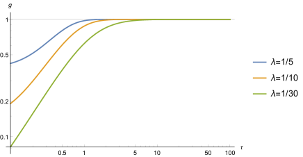
Figure 1: Plot of the spectral form factor $g(\beta,t,\hbar)$ as a function of $\tau=\hbar t$ for $\hbar=1/30$.

In Saad:2019lba it is argued that the ramp is reproduced from the genus-zero part of the connected correlator

$$\langle Z(\beta+\mathrm{i}t)Z(\beta-\mathrm{i}t)\rangle^{g=0}_{{\mbox{\scriptsize c}}}=\frac{\sqrt{\beta^{2}+t^{2}}}{4\pi\beta}=\frac{\sqrt{\lambda^{2}+\tau^{2}}}{4\pi\lambda}.$$ (155)

In Fig. 2 we show the plot of the genus-zero part (orange dashed curve) and the full result (blue solid curve) for the SFF with $\hbar=\lambda=1/30$ as an example. One can see that the genus-zero part captures the growing ramp behavior of SFF at early times. This agreement at early times can be shown analytically using the Taylor expansion of the error function and the small $\lambda$ behavior of $\mathcal{F}_{0}(\lambda)\sim\frac{\lambda^{3}}{12}$.

Figure 2: Plot of the spectral form factor for $\hbar=\lambda=1/30$. The orange dashed curve is the genus-zero result while the blue solid curve is the plot of error function.

The appearance of the plateau behavior is almost guaranteed by the functional form of the error function. However, one can pin down the origin of plateau by looking closely at the late-time behavior of the second term $\operatorname{Tr}(e^{\beta_{1}Q}\Pi e^{\beta_{2}Q}\Pi)$ in the connected correlator $Z_{2}(\beta_{1},\beta_{2})$ in (91). As we have seen in section 3.4, this term can be evaluated by the saddle point approximation. For $\beta_{1,2}=\beta\pm\mathrm{i}t$, the saddle points are given by

$$\xi_{1,2}^{*}=\frac{1}{4}\arcsin(\lambda\pm\mathrm{i}\tau)^{2},$$ (156)

and the saddle point value is given by

$$\operatorname{Tr}(e^{\beta_{1}Q}\Pi e^{\beta_{2}Q}\Pi)\sim\exp\left[\frac{\mathcal{F}_{0}(\lambda+\mathrm{i}\tau)+\mathcal{F}_{0}(\lambda-\mathrm{i}\tau)}{\hbar}\right].$$ (157)

This contribution decays exponentially at late-times and the SFF approaches the plateau value given by the first term $\operatorname{Tr}(e^{(\beta_{1}+\beta_{2})Q}\Pi)$ in (91). These saddle points (156) can be thought of as the eigenvalue instantons sitting at the complex conjugate pair of points $E=-\xi^{*}_{1,2}$ and the transition from ramp to plateau is induced by the pair creation of eigenvalue instantons as advocated in Okuyama:2018gfr .

Another interesting phenomenon is that the connected and the disconnected contributions exchange dominance as we lower the temperature. This transition is observed in a coupled SYK model Maldacena:2018lmt and it is expected to occur in JT gravity as well. To see this, let us compare the disconnected part $\langle Z(\beta)\rangle^{2}$ and the connected part $\langle Z(\beta)^{2}\rangle_{{\mbox{\scriptsize c}}}$ and study their behavior as a function of $\beta$. Here we set $\beta_{1}=\beta_{2}=\beta$ for simplicity. Since JT gravity becomes a good approximation of the SYK model in the low energy limit, it is useful to study the behavior of two-boundary correlator in the ’t Hooft limit. At the leading order in the ’t Hooft expansion we find

$$\langle Z(\beta)\rangle^{2} \approx\frac{\hbar}{4\pi(\arcsin\lambda)^{3}\sqrt{1-\lambda^{2}}}e^{\frac{2\mathcal{F}_{0}(\lambda)}{\hbar}},$$ (158)

$$\langle Z(\beta)^{2}\rangle_{{\mbox{\scriptsize c}}} \approx\sqrt{\frac{\hbar}{4\pi(\arcsin 2\lambda)^{3}\sqrt{1-4\lambda^{2}}}}e^{\frac{\mathcal{F}_{0}(2\lambda)}{\hbar}}\text{Erf}\Biggl{(}\sqrt{\frac{\mathcal{F}_{0}(2\lambda)-2\mathcal{F}_{0}(\lambda)}{\hbar}}\Biggr{)}.$$

In Fig. 3, we show the plot of (158) for $\hbar=1/30$. One can see that at high temperature the disconnected part is dominant, but as we lower the temperature the connected part becomes dominant below some critical temperature. Thus we succeeded to reproduce the transition observed in Maldacena:2018lmt directly from the JT gravity computation. In the bulk gravity picture, this is an analogue of the Hawking-Page transition between two different topologies of spacetime. At high temperature the two disconnected Euclidean black holes are dominant while at low temperature the Euclidean wormhole connecting the two boundaries becomes dominant.

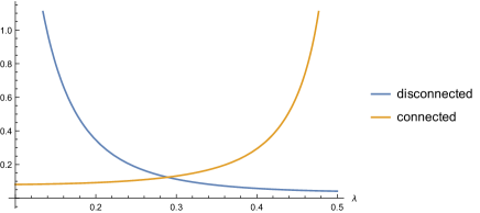
Figure 3: Plot of the disconnected part $\langle Z(\beta)\rangle^{2}$ and the connected part $\langle Z(\beta)^{2}\rangle_{{\mbox{\scriptsize c}}}$ as a function of $\lambda=\hbar\beta$ at $\hbar=1/30$.

6 Boundary creation operator and Hartle-Hawking state

As we have seen in section 2, we can write the connected $n$-point amplitude as

$$\langle Z(\beta_{1})\cdots Z(\beta_{n})\rangle_{{\mbox{\scriptsize c}}}\simeq B(\beta_{1})\cdots B(\beta_{n})F,$$ (159)

where $F$ denotes the free energy (7) and the operator $B(\beta)$ is given by (23). $B(\beta)$ can be thought of as the “boundary creation operator.” The same operator has been considered in the context of 2d gravity in Moore:1991ir . (159) should be understood as the equality up to the non-universal terms at genus-zero for the one- and two-point functions, which should be treated separately.

In a recent paper by Marolf and Maxfield Marolf:2020xie , the idea of boundary creation operators is also discussed. The important property of the boundary creation operators is that they all commute and hence can be diagonalized simultaneously. It is argued in Marolf:2020xie that the simultaneous eigenstate of the boundary creation operators, the so-called $\alpha$-state, can be thought of as a member of an ensemble and the correlator $\langle\prod_{i}Z(\beta_{i})\rangle$ is interpreted as the ensemble average. Moreover, by reinterpreting the earlier discussion of baby universes Coleman:1988cy ; Giddings:1988cx ; Giddings:1988wv from the viewpoint of AdS/CFT duality, it is argued that one can define the baby universe Hilbert space from the data of correlators $\langle\prod_{i}Z(\beta_{i})\rangle$ and this Hilbert space includes many null states due to the bulk diffeomorphism invariance. To demonstrate these properties, a simple toy model is studied in Marolf:2020xie where the action $S$ of the model has only the topological term given by the Euler characteristic $\chi$ of the 2d spacetime.

In this section we will consider whether the proposal in Marolf:2020xie can be generalized to the JT gravity case. Firstly, the boundary creation operator $B(\beta)$ defined in (23) clearly commutes

$${[}B(\beta),B(\beta^{\prime}){]}=0,$$ (160)

and hence one can try to diagonalize $B(\beta)$’s simultaneously. One immediate problem is that $B(\beta)$ in (23) does not look like a hermitian operator, thus its eigenvalue is not necessarily a real number. According to the proposal in Marolf:2020xie , this problem might be resolved on the physical Hilbert space, which is obtained by taking the quotient of the original Hilbert space by the space of null states. We do not have a clear understanding of how this happens. In the rest of this section, we will examine how the proposal of Marolf:2020xie is generalized or modified in the case of JT gravity.

To study the proposal of Marolf:2020xie in JT gravity, it is convenient to use the free boson-fermion representation of the Witten-Kontsevich $\tau$-function (see e.g. BBT ; Aganagic:2003qj ; Kostov:2009nj ; Kostov:2010nw and references therein)

$$\tau=e^{F}=\langle t|V\rangle,$$ (161)

where the state $\langle t|$ is given by the coherent state of free boson

$$\langle t|=\langle 0|\exp\left(\sum_{k=0}^{\infty}\frac{\widetilde{t}_{k}\alpha_{2k+1}}{g_{\rm s}(2k+1)!!}\right)$$ (162)

with $\alpha_{n}$ obeying the commutation relation $[\alpha_{n},\alpha_{m}]=n\delta_{n+m,0}$. $\widetilde{t}_{k}$ in (162) is defined by

$$\widetilde{t}_{k}=t_{k}-\delta_{k,1}.$$ (163)

To write down the state $|V\rangle$ in (161), it is useful to introduce the free fermions $\psi_{r},\psi_{r}^{*}~{}(r\in\mathbb{Z}+\frac{1}{2})$ obeying the anti-commutation relation $\{\psi_{r},\psi_{s}^{*}\}=\delta_{r+s,0}$. Then $|V\rangle$ is written as

$$|V\rangle=\exp\left(\sum_{m,n=0}^{\infty}A_{m,n}\psi_{-m-\frac{1}{2}}\psi^{*}_{-n-\frac{1}{2}}\right)|0\rangle.$$ (164)

The generating function of $A_{m,n}$ for the Witten-Kontsevich $\tau$-function is obtained in zhou2013explicit ; zhou2015emergent ; balogh2017geometric . The important property of the state $|V\rangle$ is that it satisfies the Virasoro constraint Fukuma:1990jw ; Dijkgraaf:1990rs

$$\mathcal{L}_{n}|V\rangle=0\quad(n\geq-1),$$ (165)

where the Virasoro generator $\mathcal{L}_{n}$ is given by

$$\mathcal{L}_{n} =\frac{1}{4}\sum_{k\in\mathbb{Z}}:\alpha_{2k+1}\alpha_{2n-2k-1}:-\frac{1}{2g_{\rm s}}\alpha_{2n+3}+\frac{1}{16}\delta_{n,0}.$$ (166)

In Sen:1990rz ; Imbimbo:1990ua , the Virasoro constraint of matrix model is interpreted as the gauge symmetry of closed string field theory in a minimal model background. This suggests that the Virasoro constraint is the analogue of the bulk diffeomorphism invariance discussed in Marolf:2020xie .

Now let us consider the Hartle-Hawking state $|\text{HH}\rangle$ Hartle:1983ai . As discussed in Polchinski:1989fn , it is natural to identify the Hartle-Hawking state $|\text{HH}\rangle$ as “the most symmetric state.” In the present case, $|V\rangle$ is such a state since $|V\rangle$ is invariant under the Virasoro generators (166). $|V\rangle$ can be thought of as the $SL(2,\mathbb{C})$ invariant vacuum corresponding to the identity operator and it is a natural candidate for the no-boundary state. Thus we propose to identify the Hartle-Hawking state $|\text{HH}\rangle$ with the state $|V\rangle$ in (164)

$$|\text{HH}\rangle=|V\rangle.$$ (167)

In particular, this state satisfies the equation $\mathcal{L}_{0}|\text{HH}\rangle=0$ which corresponds to the Wheeler-DeWitt equation.

Next we consider the interpretation of the correlator $\langle\prod_{i}Z(\beta_{i})\rangle$ in JT gravity. The correlator here refers to the full correlator including both the connected and the disconnected parts. One can generalize (159) to the full correlator by acting $B(\beta)$’s on the $\tau$-function instead of the free energy

$$\langle Z(\beta_{1})\cdots Z(\beta_{n})\rangle \simeq\frac{B(\beta_{1})\cdots B(\beta_{n})\langle t|V\rangle}{\langle t|V\rangle}$$ (168)

$$=:\frac{\langle t|\widehat{B}(\beta_{1})\cdots\widehat{B}(\beta_{n})|V\rangle}{\langle t|V\rangle},$$

where the operator $\widehat{B}(\beta)$ is written as

$$\widehat{B}(\beta)=\frac{1}{\sqrt{2\pi}}\sum_{n=0}^{\infty}\frac{\beta^{n+\frac{1}{2}}}{(2n+1)!!}\alpha_{2n+1}.$$ (169)

It turns out that the non-universal terms at genus-zero are correctly incorporated by extending the summation to all $n\in\mathbb{Z}$. Namely we define the operator $\widehat{Z}(\beta)$ by

$$\widehat{Z}(\beta)=\frac{1}{\sqrt{2\pi}}\sum_{n=-\infty}^{\infty}\frac{\beta^{n+\frac{1}{2}}}{(2n+1)!!}\alpha_{2n+1}.$$ (170)

Then the full correlator is given by

$$\langle Z(\beta_{1})\cdots Z(\beta_{n})\rangle=\frac{\langle t|\widehat{Z}(\beta_{1})\cdots\widehat{Z}(\beta_{n})|\text{HH}\rangle}{\langle t|\text{HH}\rangle},$$ (171)

where we used our identification $|\text{HH}\rangle=|V\rangle$. To see that this is the correct prescription, let us consider the genus-zero part of the one-point function

$$\langle Z(\beta)\rangle^{g=0} =\frac{\langle t|\widehat{Z}(\beta)|\text{HH}\rangle}{\langle t|\text{HH}\rangle}\Bigg{|}_{g=0}=\langle 0|\exp\left(\sum_{k=1}^{\infty}\frac{\widetilde{t}_{k}}{g_{\rm s}(2k+1)!!}\alpha_{2k+1}\right)\widehat{Z}(\beta)|0\rangle$$ (172)

$$=\frac{1}{\sqrt{2\pi}g_{\rm s}}\sum_{k=1}^{\infty}\beta^{-k-\frac{1}{2}}\frac{\widetilde{t}_{k}}{(2k-1)!!(-2k-1)!!}$$

$$=\frac{e^{1/\beta}}{\sqrt{2\pi}g_{\rm s}\beta^{3/2}}.$$

Here we have used $\widetilde{t}_{k}=\frac{(-1)^{k}}{(k-1)!}~{}(k\geq 1)$ and

$$(2k-1)!!(-2k-1)!!=(-1)^{k}.$$ (173)

Similarly, the genus-zero part of the two-point function becomes

$$\langle Z(\beta_{1})Z(\beta_{2})\rangle^{g=0}_{{\mbox{\scriptsize c}}} =\frac{1}{2\pi}\Biggl{\langle}0\Biggr{|}\sum_{k=0}^{\infty}\frac{\beta_{1}^{k+\frac{1}{2}}}{(2k+1)!!}\alpha_{2k+1}\sum_{n=0}^{\infty}\frac{\beta_{2}^{-n-\frac{1}{2}}}{(-2n-1)!!}\alpha_{-2n-1}\Biggl{|}0\Biggr{\rangle}$$ (174)

$$=\frac{1}{2\pi}\sum_{n=0}^{\infty}\frac{\beta_{1}^{n+\frac{1}{2}}\beta_{2}^{-n-\frac{1}{2}}}{(2n-1)!!(-2n-1)!!}$$

$$=\frac{\sqrt{\beta_{1}\beta_{2}}}{2\pi(\beta_{1}+\beta_{2})}.$$

(172) and (174) agree with the known result of the genus-zero part in JT gravity. Using the relation (173) one can show that $\widehat{Z}(\beta)$’s commute at least formally

$${[}\widehat{Z}(\beta_{1}),\widehat{Z}(\beta_{2}){]} =\frac{1}{2\pi}\sum_{n,k\geq 0}\left[\frac{\beta_{1}^{k+\frac{1}{2}}}{(2k+1)!!}\alpha_{2k+1},\frac{\beta_{2}^{-n-\frac{1}{2}}}{(-2n-1)!!}\alpha_{-2n-1}\right]$$ (175)

$$+\frac{1}{2\pi}\sum_{n,k\geq 0}\left[\frac{\beta_{1}^{-k-\frac{1}{2}}}{(-2k-1)!!}\alpha_{-2k-1},\frac{\beta_{2}^{n+\frac{1}{2}}}{(2n+1)!!}\alpha_{2n+1}\right]$$

$$=\frac{1}{2\pi}\sum_{n\geq 0}(-1)^{n}\Bigl{(}\beta_{1}^{n+\frac{1}{2}}\beta_{2}^{-n-\frac{1}{2}}-\beta_{1}^{-n-\frac{1}{2}}\beta_{2}^{n+\frac{1}{2}}\Bigr{)}$$

$$=\frac{\sqrt{\beta_{1}\beta_{2}}}{2\pi}\left(\frac{1}{\beta_{1}+\beta_{2}}-\frac{1}{\beta_{1}+\beta_{2}}\right)$$

$$=0.$$

Our proposal (171) is consistent with the identification of the one-point function $\langle Z(\beta)\rangle$ as the wavefunction of the Hartle-Hawking state, which is usually assumed in 2d gravity literature (see e.g. Ginsparg:1993is and references therein)

$$\langle Z(\beta)\rangle=\Psi_{\text{HH}}(\beta)=\langle\beta|\text{HH}\rangle,$$ (176)

where $\langle\beta|$ is given by

$$\langle\beta|=\frac{\langle t|\widehat{Z}(\beta)}{\langle t|\text{HH}\rangle}.$$ (177)

More generally, the multi-point correlator is written as

$$\langle Z(\beta_{1})\cdots Z(\beta_{n})\rangle =\langle\beta_{1},\cdots,\beta_{n}|\text{HH}\rangle,$$ (178)

$$\langle\beta_{1},\cdots,\beta_{n}| =\frac{\langle t|\widehat{Z}(\beta_{1})\cdots\widehat{Z}(\beta_{n})}{\langle t|\text{HH}\rangle}.$$

Our expression (171) is different from the proposal in Marolf:2020xie

$$\langle Z(\beta_{1})\cdots Z(\beta_{n})\rangle=\frac{\langle\text{HH}|\widehat{Z}(\beta_{1})\cdots\widehat{Z}(\beta_{n})|\text{HH}\rangle}{\langle\text{HH}|\text{HH}\rangle}.$$ (179)

This difference comes from the fact that the bra and the ket are treated asymmetrically in the free boson/fermion representation of the $\tau$-function (161). In other words, our expression (171) corresponds to a special (Euclidean) time-slicing of the spacetime where the initial state has no boundary and all the boundaries are on the final state. At present, it is not clear to us how to reconcile our (171) and the proposal (179) in Marolf:2020xie .

7 Conclusions and outlook

We have studied the multi-boundary correlators in JT gravity using the KdV constraints obeyed by these correlators. Along the way, we have defined the off-shell generalization of the effective potential and have studied the WKB expansion of the Baker-Akhiezer functions as well. In particular, we have computed the genus expansion of the connected two-boundary correlator $\langle Z(\beta_{1})Z(\beta_{2})\rangle_{\mbox{\scriptsize c}}$ as well as its low temperature expansion. We have found that the two-point function is written in terms of the error function and the ramp and plateau behavior of the SFF in JT gravity is explained by the functional form of this error function. We have also confirmed the picture put forward in Okuyama:2018gfr that the transition from ramp to plateau is induced by the pair creation of eigenvalue instantons.

There are many interesting open questions. In section 6 we briefly discussed a possible connection to the recent work by Marolf and Maxfield Marolf:2020xie which clearly deserves further investigation. It would be interesting to construct the $\alpha$-state which simultaneously diagonalizes the operator $\widehat{Z}(\beta)$ in (170) and see how the argument in Marolf:2020xie is generalized to the JT gravity case. In particular, it is interesting to see what the non-factorized contribution $\langle Z(\beta_{1})Z(\beta_{2})\rangle_{\mbox{\scriptsize c}}$ coming from the Euclidean wormhole Maldacena:2004rf ; ArkaniHamed:2007js looks like in the $\alpha$-state. The pure topological gravity would be a good starting point to study this problem since the explicit form of the $n$-point correlator is known in the literature okounkov2002generating ; buryak ; Alexandrov:2019eah .

It is emphasized in Marolf:2020xie that non-perturbative effects are important to realize the massive truncation of the Hilbert space by the diffeomorphism invariance. The free fermion representation of the state $|V\rangle$ in (164) is defined by the asymptotic expansion in $g_{\rm s}$ and hence it only makes sense as a perturbative expansion. However, it is possible to include the effect of D-instanton corrections systematically within this framework Fukuma:1996hj ; Fukuma:1996bq ; Fukuma:1999tj . It would be interesting to study such D-instanton effects in JT gravity and see how they affect the argument of diffeomorphism invariance in JT gravity.

In Penington:2019kki ; Almheiri:2019qdq it is argued that the Page curve for the black hole evaporation is correctly reproduced if we include the contribution of replica wormholes in the computation of entropy of Hawking radiation using the replica method in the gravity path integral. One can immediately apply our formalism to compute the contribution of the replica wormholes in pure JT gravity sector. To model the black hole microstates one can add the end of the world (EOW) branes to JT gravity Penington:2019kki ; Marolf:2020xie . It would be interesting to construct a generalization of the JT gravity matrix model which incorporates the degrees of freedom of the EOW branes.

As discussed in Maldacena:2019cbz ; Cotler:2019nbi , the matrix model description of JT gravity can be generalized to the 2d de Sitter space by analytically continuing the boundary length $\beta$ to imaginary value $\beta\to\pm\mathrm{i}\ell$. In Cotler:2019dcj the boundary creation/annihilation operators are considered in this de Sitter setting. It would be interesting to see how they are related to our discussion in section 6.

Finally, it would be interesting to generalize our computation in this paper to JT supergravity Stanford:2019vob . In particular, the genus expansion of JT supergravity on orientable surfaces without time-reversal symmetry can be computed from the Brezin-Gross-Witten $\tau$-function norbury . We will report on the computation of JT supergravity case elsewhere.

Appendix A Wavefunction of microscopic loop operators

In this appendix we will consider the correlator of microscopic loop operators in the presence of one macroscopic loop operator. It is easily obtained by differentiating $\langle Z(\beta)\rangle$

$$\partial_{n_{1}}\partial_{n_{2}}\cdots\langle Z(\beta)\rangle=\langle\tau_{n_{1}}\tau_{n_{2}}\cdots Z(\beta)\rangle.$$ (180)

It is convenient to define the normalized correlator

$$\big{\langle}\!\big{\langle}\prod_{i}\tau_{n_{i}}\big{\rangle}\!\big{\rangle}:=\frac{\langle\prod_{i}\tau_{n_{i}}Z(\beta)\rangle}{\langle Z(\beta)\rangle},$$ (181)

which can be thought of as the wavefunction of microscopic loop operators Moore:1991ir ; Ginsparg:1993is .

For instance, the one-point function $\big{\langle}\!\big{\langle}\tau_{n}\big{\rangle}\!\big{\rangle}$ at the leading order is given by

$$\big{\langle}\!\big{\langle}\tau_{n}\big{\rangle}\!\big{\rangle}=\partial_{n}\log\langle Z(\beta)\rangle\approx\frac{1}{\hbar}\partial_{n}\mathcal{F}_{0}(\lambda).$$ (182)

The derivative of $\mathcal{F}_{0}(\lambda)$ with respect to the coupling $t_{n}$ can be computed by using the fact that $V_{\text{eff}}(\xi)$ and $\mathcal{F}_{0}(\lambda)$ are related by the Legendre transformation. Thus we find

$$\frac{\partial\mathcal{F}_{0}(\lambda)}{\partial t_{n}}\Bigg{|}_{\lambda~{}\text{fixed}} =\frac{\partial}{\partial t_{n}}\Bigg{|}_{\lambda~{}\text{fixed}}\Bigl{(}\lambda\xi_{*}-V_{\text{eff}}(\xi_{*})\Bigr{)}$$ (183)

$$=\lambda\frac{\partial\xi_{*}}{\partial t_{n}}-V_{\text{eff}}^{\prime}(\xi_{*})\frac{\partial\xi_{*}}{\partial t_{n}}-\frac{\partial V_{\text{eff}}(\xi_{*})}{\partial t_{n}}\Bigg{|}_{\xi_{*}~{}\text{fixed}}$$

$$=-\frac{\partial V_{\text{eff}}(\xi_{*})}{\partial t_{n}}\Bigg{|}_{\xi_{*}~{}\text{fixed}}.$$

In the last step we have used the saddle point equation $\lambda=V_{\text{eff}}^{\prime}(\xi_{*})$. From the explicit form of the off-shell effective potential in (84), one can easily compute the derivative $-\partial_{n}V_{\text{eff}}(\xi_{*})$. From (182) and (183), for the on-shell JT gravity case $t_{n}=\gamma_{n}$ we find the wavefunction of the microscopic loop operator $\tau_{n}$ at the leading order in the ’t Hooft expansion (2)

$$\big{\langle}\!\big{\langle}\tau_{n}\big{\rangle}\!\big{\rangle}=\frac{\arcsin(\lambda)^{2n+1}}{2^{n}(2n+1)!!\hbar}+\mathcal{O}(\hbar^{0}).$$ (184)

It turns out that the wavefunction is factorized at the leading order in the ’t Hooft expansion

$$\big{\langle}\!\big{\langle}\prod_{i}\tau_{n_{i}}\big{\rangle}\!\big{\rangle} \approx e^{-\frac{\mathcal{F}_{0}(\lambda)}{\hbar}}\prod_{i}\partial_{n_{i}}e^{\frac{\mathcal{F}_{0}(\lambda)}{\hbar}}$$ (185)

$$\approx\prod_{i}\frac{\partial_{n_{i}}\mathcal{F}_{0}(\lambda)}{\hbar}$$

$$\approx\prod_{i}\big{\langle}\!\big{\langle}\tau_{n_{i}}\big{\rangle}\!\big{\rangle}.$$

One can go beyond the leading order and compute the higher order correction to the wavefunction of microscopic loop operators by using the off-shell generalization of the free energy $\mathcal{F}$ in (109). After some algebra, we find the first order correction to the ’t Hooft expansion

$$\big{\langle}\!\big{\langle}\tau_{0}^{k}\prod_{i=1}^{m}\tau_{n_{i}}\big{\rangle}\!\big{\rangle}= \frac{\arcsin(\lambda)^{k}}{\hbar^{m+k}}\prod_{i=1}^{m}\frac{\arcsin(\lambda)^{2n_{i}+1}}{2^{n_{i}}(2n_{i}+1)!!}$$ (186)

$$\times \Biggl{[}1+\hbar\biggl{(}2\sum_{i=1}^{m}n_{i}+m+k\biggr{)}\left(\frac{2\sum_{i=1}^{m}n_{i}+m+k-5}{\sqrt{1-\lambda^{2}}\arcsin(\lambda)^{3}}+\frac{\lambda}{(1-\lambda^{2})\arcsin(\lambda)^{2}}\right)$$

$$\qquad+\hbar\frac{5k-k^{2}}{\arcsin(\lambda)^{3}}+\mathcal{O}(\hbar^{2})\Biggr{]},$$

where $n_{i}>0~{}(i=1,\cdots,m)$.

References

- (1) R. Jackiw, “Lower Dimensional Gravity,” Nucl. Phys. B252 (1985) 343–356.
- (2) C. Teitelboim, “Gravitation and Hamiltonian Structure in Two Space-Time Dimensions,” Phys. Lett. 126B (1983) 41–45.
- (3) A. Almheiri and J. Polchinski, “Models of AdS2 backreaction and holography,” JHEP 11 (2015) 014, arXiv:1402.6334 [hep-th].
- (4) J. Maldacena, D. Stanford, and Z. Yang, “Conformal symmetry and its breaking in two dimensional Nearly Anti-de-Sitter space,” PTEP 2016 no. 12, (2016) 12C104, arXiv:1606.01857 [hep-th].
- (5) K. Jensen, “Chaos in AdS2 Holography,” Phys. Rev. Lett. 117 no. 11, (2016) 111601, arXiv:1605.06098 [hep-th].
- (6) J. Engelsöy, T. G. Mertens, and H. Verlinde, “An investigation of AdS2 backreaction and holography,” JHEP 07 (2016) 139, arXiv:1606.03438 [hep-th].
- (7) S. Sachdev and J. Ye, “Gapless Spin-Fluid Ground State in a Random Quantum Heisenberg Magnet,” Phys. Rev. Lett. 70 (2018) 3339, arXiv:cond-mat/9212030.
- (8) A. Kitaev, “A simple model of quantum holography (part 1 and 2),”. Talks at KITP on April 7, 2015 and May 27, 2015.
- (9) P. Saad, S. H. Shenker, and D. Stanford, “JT gravity as a matrix integral,” arXiv:1903.11115 [hep-th].
- (10) D. Stanford and E. Witten, “JT Gravity and the Ensembles of Random Matrix Theory,” arXiv:1907.03363 [hep-th].
- (11) A. Blommaert, T. G. Mertens, and H. Verschelde, “Eigenbranes in Jackiw-Teitelboim gravity,” arXiv:1911.11603 [hep-th].
- (12) K. Okuyama and K. Sakai, “JT gravity, KdV equations and macroscopic loop operators,” JHEP 01 (2020) 156, arXiv:1911.01659 [hep-th].
- (13) C. V. Johnson, “Non-Perturbative JT Gravity,” arXiv:1912.03637 [hep-th].
- (14) D. Kapec, R. Mahajan, and D. Stanford, “Matrix ensembles with global symmetries and ’t Hooft anomalies from 2d gauge theory,” arXiv:1912.12285 [hep-th].
- (15) P. Betzios and O. Papadoulaki, “Liouville theory and Matrix models: A Wheeler DeWitt perspective,” arXiv:2004.00002 [hep-th].
- (16) B. Eynard and N. Orantin, “Invariants of algebraic curves and topological expansion,” Commun. Num. Theor. Phys. 1 (2007) 347–452, arXiv:math-ph/0702045 [math-ph].
- (17) E. Witten, “Two-dimensional gravity and intersection theory on moduli space,” Surveys Diff. Geom. 1 (1991) 243–310.
- (18) M. Kontsevich, “Intersection theory on the moduli space of curves and the matrix Airy function,” Commun. Math. Phys. 147 (1992) 1–23.
- (19) T. Banks, M. R. Douglas, N. Seiberg, and S. H. Shenker, “Microscopic and Macroscopic Loops in Nonperturbative Two-dimensional Gravity,” Phys. Lett. B238 (1990) 279.
- (20) P. Zograf, “On the large genus asymptotics of Weil-Petersson volumes,” arXiv:0812.0544 [math.AG].
- (21) M. Mirzakhani, “Simple geodesics and Weil-Petersson volumes of moduli spaces of bordered Riemann surfaces,” Invent. Math. 167 no. 1, (2007) 179–222.
- (22) L. V. Iliesiu and G. J. Turiaci, “The statistical mechanics of near-extremal black holes,” arXiv:2003.02860 [hep-th].
- (23) G. W. Moore, N. Seiberg, and M. Staudacher, “From loops to states in 2-D quantum gravity,” Nucl. Phys. B362 (1991) 665–709.
- (24) P. H. Ginsparg and G. W. Moore, “Lectures on 2-D gravity and 2-D string theory,” in Proceedings, Theoretical Advanced Study Institute (TASI 92): From Black Holes and Strings to Particles: Boulder, USA, June 1-26, 1992. arXiv:hep-th/9304011 [hep-th].
- (25) A. Okounkov, “Generating functions for intersection numbers on moduli spaces of curves,” International Mathematics Research Notices 2002 no. 18, (2002) 933–957, arXiv:math/0101201 [math.AT].
- (26) P. Saad, S. H. Shenker, and D. Stanford, “A semiclassical ramp in SYK and in gravity,” arXiv:1806.06840 [hep-th].
- (27) A. M. García-García and J. J. M. Verbaarschot, “Spectral and thermodynamic properties of the Sachdev-Ye-Kitaev model,” Phys. Rev. D94 no. 12, (2016) 126010, arXiv:1610.03816 [hep-th].
- (28) J. S. Cotler, G. Gur-Ari, M. Hanada, J. Polchinski, P. Saad, S. H. Shenker, D. Stanford, A. Streicher, and M. Tezuka, “Black Holes and Random Matrices,” JHEP 05 (2017) 118, arXiv:1611.04650 [hep-th]. [Erratum: JHEP09,002(2018)].
- (29) P. Saad, “Late Time Correlation Functions, Baby Universes, and ETH in JT Gravity,” arXiv:1910.10311 [hep-th].
- (30) D. Marolf and H. Maxfield, “Transcending the ensemble: baby universes, spacetime wormholes, and the order and disorder of black hole information,” arXiv:2002.08950 [hep-th].
- (31) S. R. Coleman, “Black Holes as Red Herrings: Topological Fluctuations and the Loss of Quantum Coherence,” Nucl. Phys. B307 (1988) 867–882.
- (32) S. B. Giddings and A. Strominger, “Loss of Incoherence and Determination of Coupling Constants in Quantum Gravity,” Nucl. Phys. B307 (1988) 854–866.
- (33) S. B. Giddings and A. Strominger, “Baby Universes, Third Quantization and the Cosmological Constant,” Nucl. Phys. B321 (1989) 481–508.
- (34) M. Mulase and B. Safnuk, “Mirzakhani’s recursion relations, Virasoro constraints and the KdV hierarchy,” arXiv:math/0601194 [math].
- (35) R. Dijkgraaf and E. Witten, “Developments in Topological Gravity,” Int. J. Mod. Phys. A33 no. 30, (2018) 1830029, arXiv:1804.03275 [hep-th].
- (36) C. Itzykson and J. B. Zuber, “Combinatorics of the modular group. 2. The Kontsevich integrals,” Int. J. Mod. Phys. A7 (1992) 5661–5705, arXiv:hep-th/9201001.
- (37) J. Ambjorn, J. Jurkiewicz, and Yu. M. Makeenko, “Multiloop correlators for two-dimensional quantum gravity,” Phys. Lett. B251 (1990) 517–524.
- (38) I. Gelfand and L. Dikii, “Asymptotic behavior of the resolvent of Sturm-Liouville equations and the algebra of the Korteweg-De Vries equations,” Russ. Math. Surveys 30 no. 5, (1975) 77–113.
- (39) O. Babelon, D. Bernard, and M. Talon, Introduction to Classical Integrable Systems. Cambridge University Press, 2007.
- (40) K. Okuyama, “Connected correlator of 1/2 BPS Wilson loops in SYM,” JHEP 10 (2018) 037, arXiv:1808.10161 [hep-th].
- (41) K. Okuyama, “Eigenvalue instantons in the spectral form factor of random matrix model,” JHEP 03 (2019) 147, arXiv:1812.09469 [hep-th].
- (42) J. Maldacena and X.-L. Qi, “Eternal traversable wormhole,” arXiv:1804.00491 [hep-th].
- (43) J. McNamara and C. Vafa, “Baby Universes, Holography, and the Swampland,” arXiv:2004.06738 [hep-th].
- (44) M. Aganagic, R. Dijkgraaf, A. Klemm, M. Marino, and C. Vafa, “Topological strings and integrable hierarchies,” Commun. Math. Phys. 261 (2006) 451–516, arXiv:hep-th/0312085.
- (45) I. Kostov, “Matrix models as CFT: Genus expansion,” Nucl. Phys. B837 (2010) 221–238, arXiv:0912.2137 [hep-th].
- (46) I. Kostov and N. Orantin, “CFT and topological recursion,” JHEP 11 (2010) 056, arXiv:1006.2028 [hep-th].
- (47) J. Zhou, “Explicit formula for Witten-Kontsevich tau-function,” arXiv:1306.5429 [math.AG].
- (48) J. Zhou, “Emergent geometry and mirror symmetry of a point,” arXiv:1507.01679 [math-ph].
- (49) F. Balogh and D. Yang, “Geometric interpretation of Zhou’s explicit formula for the Witten–Kontsevich tau function,” Letters in Mathematical Physics 107 no. 10, (2017) 1837–1857, arXiv:1412.4419 [math-ph].
- (50) M. Fukuma, H. Kawai, and R. Nakayama, “Continuum Schwinger-dyson Equations and Universal Structures in Two-dimensional Quantum Gravity,” Int. J. Mod. Phys. A6 (1991) 1385–1406.
- (51) R. Dijkgraaf, H. L. Verlinde, and E. P. Verlinde, “Loop equations and Virasoro constraints in nonperturbative 2-D quantum gravity,” Nucl. Phys. B348 (1991) 435–456.
- (52) A. Sen, “Virasoro constraints on the matrix model partition function and string field theory,” Int. J. Mod. Phys. A7 (1992) 1553–1581.
- (53) C. Imbimbo and S. Mukhi, “String field theory in minimal model backgrounds and nonperturbative two-dimensional gravity,” Nucl. Phys. B364 (1991) 662–680.
- (54) J. B. Hartle and S. W. Hawking, “Wave Function of the Universe,” Phys. Rev. D28 (1983) 2960–2975.
- (55) J. Polchinski, “A Two-Dimensional Model for Quantum Gravity,” Nucl. Phys. B324 (1989) 123–140.
- (56) J. M. Maldacena and L. Maoz, “Wormholes in AdS,” JHEP 02 (2004) 053, arXiv:hep-th/0401024 [hep-th].
- (57) N. Arkani-Hamed, J. Orgera, and J. Polchinski, “Euclidean wormholes in string theory,” JHEP 12 (2007) 018, arXiv:0705.2768 [hep-th].
- (58) A. Buryak, “Double ramification cycles and the -point function for the moduli space of curves,” arXiv:1605.03736 [math.AG].
- (59) A. Alexandrov, F. Hernández Iglesias, and S. Shadrin, “Buryak-Okounkov formula for the -point function and a new proof of the Witten conjecture,” arXiv:1902.03160 [math.AG].
- (60) M. Fukuma and S. Yahikozawa, “Nonperturbative effects in noncritical strings with soliton backgrounds,” Phys. Lett. B396 (1997) 97–106, arXiv:hep-th/9609210.
- (61) M. Fukuma and S. Yahikozawa, “Combinatorics of solitons in noncritical string theory,” Phys. Lett. B393 (1997) 316–320, arXiv:hep-th/9610199 [hep-th].
- (62) M. Fukuma and S. Yahikozawa, “Comments on D instantons in strings,” Phys. Lett. B460 (1999) 71–78, arXiv:hep-th/9902169 [hep-th].
- (63) G. Penington, S. H. Shenker, D. Stanford, and Z. Yang, “Replica wormholes and the black hole interior,” arXiv:1911.11977 [hep-th].
- (64) A. Almheiri, T. Hartman, J. Maldacena, E. Shaghoulian, and A. Tajdini, “Replica Wormholes and the Entropy of Hawking Radiation,” arXiv:1911.12333 [hep-th].
- (65) J. Maldacena, G. J. Turiaci, and Z. Yang, “Two dimensional Nearly de Sitter gravity,” arXiv:1904.01911 [hep-th].
- (66) J. Cotler, K. Jensen, and A. Maloney, “Low-dimensional de Sitter quantum gravity,” arXiv:1905.03780 [hep-th].
- (67) J. Cotler and K. Jensen, “Emergent unitarity in de Sitter from matrix integrals,” arXiv:1911.12358 [hep-th].
- (68) P. Norbury, “A new cohomology class on the moduli space of curves,” arXiv:1712.03662 [math.AG].