General Mapping between
Complex Spatial and Temporal Frequencies
by Analytical Continuation

Abstract

This paper introduces a general technique for inter-mapping the complex spatial frequency (or propagation constant) $\gamma=\alpha+j\beta$ and the temporal frequency $\omega=\omega_{\text{r}}+j\omega_{\text{i}}$ of an arbitrary electromagnetic structure. This technique, based on the analytic property of complex functions describing physical phenomena, invokes the analytic continuity theorem to assert the unicity of the mapping function, and find this function from known data within a restricted domain of its analycity by curve-fitting to a generic polynomial expansion. It is not only applicable to canonical problems admitting an analytical solution, but to any problems, from eigen-mode or driven-mode full-wave simulation results. The proposed technique is demonstrated for several systems, namely an unbounded lossy medium, a dielectric-filled rectangular waveguide, a periodically-loaded transmission line, a one-dimensional photonic crystal and a series-fed patch (SFP) leaky-wave antenna (LWA), and it is validated either by analytical results or by full-wave simulated results.

I Introduction

Waves propagate in both space and time. They are therefore characterized by both spatial and temporal frequencies [1, 2]. The spatial frequency, $\mathbf{k}$ (vector), or inverse space, and the temporal frequency, $\omega$ (scalar), or inverse time, are the Fourier counterparts of the position, $\mathbf{r}$ (vector), or direct space, and time, $t$ (scalar), or direct time, respectively, where the terms ‘direct’ and ‘inverse’ refer to the independent variables of the usual Fourier transform-pair [3, 4]. The spatial and temporal spectra are properties of waves that are as fundamental as their direct-space features [4, 5, 6, 7].

Although these spatial and temporal frequencies are generally complex, and may therefore be written as

$$k=\beta-j\alpha=-j\gamma$$ (1a)

and

$$\omega=\omega_{\text{r}}+j\omega_{\text{i}}=2\pi(f_{\text{r}}+jf_{\text{i}}),$$ (1b)

where we have temporarily reduced the vector $\mathbf{k}$ to a scalar, $k$, for simplicity, they are most often not simultaneously complex. Depending on the excitation, we typically have $\omega$ real and $k$ complex or $k$ real and $\omega$ complex. In the Traveling-Wave (TW) regime, as for instance for propagation in an unbounded medium or in a matched waveguide, the temporal frequency is purely real and the spatial frequency is complex, i.e.,

$$\omega=\omega_{\text{r}}$$ (2a)

and

$$k=\beta-j\alpha,$$ (2b)

while in the Standing-Wave (SW) regime, as for instance for propagation in a bounded medium, in a terminated waveguide or in a resonant scatterer, the spatial frequency is purely real and the temporal frequency is complex, i.e.,

$$k=\beta$$ (3a)

and

$$\omega=\omega_{\text{r}}+j\omega_{\text{i}}.$$ (3b)

The difference between the natures of the frequencies involved in the TW regime [Eq. (2)] and in SW regime [Eq. (3)], raises the following fundamental question: Can one, for a given system, systematically find the correspondence between the TW-regime quantities ($\omega_{\text{r}}$, $\beta$, $\alpha$) and the SW-regime quantities ($\beta$, $\omega_{\text{r}}$, $\omega_{\text{i}}$), and vice versa? The answer to this question is positive, and it is the object of this paper to demonstrate this fact and to provide a mapping technique applicable to any electromagnetic system.

In fact, this question originally occurred to the mind of the second author, about 15 years ago, in connection with periodic leaky-wave antenna (LWA) structures [10]. Whereas a periodic LWA is typically operated in the TW-regime, and hence characterized by the triplet ($\omega_{\text{r}}$, $\beta$, $\alpha$), it is most conveniently analyzed in the SW-regime, or more precisely in the Periodic Boundary Condition (PBC) regime, characterized by the triplet ($\beta$, $\omega_{\text{r}}$, $\omega_{\text{i}}$), with $\omega_{\text{i}}\neq{0}$ in the fast-wave region of the dispersion diagram, even in the absence of dissipative loss, due to leakage. How could one obtain the useful former triplet, where $\alpha$ represents the leakage factor of the antenna, from the computed latter triplet, where $\omega_{\text{i}}=1/\tau=\omega_{0}/(2Q)$, with $\tau$ being the relaxation time, $\omega_{0}$ the resonance frequency and $Q$ the related unloaded quality factor [11]?

In the periodic LWA problem, the dispersion parameters, ($\omega_{\text{r}}$, $\beta$, $\alpha$), of the infinite structure or, equivalently, of the matched structure, may be computed in the TW-regime by simulating the actual periodic LWA structure as a two-port network with $N$ unit cells, without any dissipative loss, so that all the simulated loss accounts for radiation only, and computing $\beta$ and $\alpha$ versus the excitation frequency, $\omega_{\text{r}}$, as $\beta=-\varphi^{\text{uw}}\left\{S_{21}\right\}/\ell$ and $\alpha=-\ln(|S_{21}|/\sqrt{1-|S_{11}|^{2}})/\ell$, respectively, where $S_{21}$ and $S_{11}$ are the transmission and reflection scattering parameters of the two-port waveguiding structure, $\varphi^{\text{uw}}$ denotes the unwrapped phase [12], and $\ell=Np$, with $p$ being the period, is the total length of the structure. Such a driven-mode procedure, used for instance in [13], is very inefficient, not only because it requires the simulation of $N$ identical cells, but also because it requires increasing the number of cells as $N\rightarrow{N+1}$ until the computed $\beta(\omega)$ and $\alpha(\omega)$ have converged to their final periodic value In contrast, the PBC-regime eigen-mode problem only necessitate the computation of the (unique) periodic cell, which is much faster, but, unfortunately, delivers the awkward triplet ($\beta$, $\omega_{\text{r}}$, $\omega_{\text{i}}$) instead of the desired triplet ($\omega_{\text{r}}$, $\beta$, $\alpha$)!

A relation between the complex temporal and spatial frequencies for periodic structures was first reported in [14], and an attempt to find a general mapping solution, starting with the simplest problem of plane-wave propagation in an unbounded lossy medium, was discussed in [15]. The topic was recently revisited in [16], where a mapping relation was derived for the problem of a (closed) waveguide. However, all these studies are restricted to problems having a known analytical solution. Such solutions are therefore simple, because they just result from inverting an analytical function, but they are of limited practical interest since only a few canonical structures admit an analytical solution, whereas virtually all practical engineering structures can be simulated only numerically.

This paper resolves the long-lasting problem of the general mapping between the complex spatial and temporal frequencies of electromagnetic structures, without requiring an analytical solution. It shows that, based on the theorem of analytical continuation and on the physical nature of real phenomena, the mapping function between the two complex spaces is necessarily unique, and presents a general technique for determining and inverting this function, using a general polynomial approximation of the function with fitted parameters. This method applies to any structure, periodic or nonperiodic, with simulated triplets ($\omega_{\text{r}}$, $\beta$, $\alpha$) or ($\beta$, $\omega_{\text{r}}$, $\omega_{\text{i}}$), and systematically allows to convert one to the other.

The paper is organized as follows. Section II explains the concept of complex frequencies (usual frequency and propagation constant) and the problem. Section III gives examples of problems with analytical solutions, as later benchmarks for the proposed method. Section IV presents the proposed general mapping technique, based on the analytical continuation theorem and polynomial curve-fitting. Section V provides a numerical validation and illustration of the method for various examples, including the periodic LWA at the origin of this research. Finally, Sec. VI closes the paper.

II Statement of the Problem

This section first describes the complex spatial frequency [Eq. (1a)] and the complex temporal frequency [Eq. (1b)], and then states the general plane mapping problem between them.

II-A Complex Spatial and Temporal Frequencies

We shall consider here a periodic problem, because such a problem is also a generalization of a non-periodic problem and because it best relates to the original problem of the periodic LWA. We assume a one-dimensional periodic structure of periodicity $p$ and composed of arbitrarily-shaped unit particles (e.g., spheres), as shown in Fig. 1.

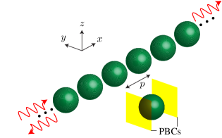
Figure 1: Generic one-dimensional periodic structure.

The driven-mode analysis procedure excites a finite ($N$-cell) version of the periodic structure at one of its ends with a harmonic wave of a given real temporal frequency, or frequency, $\omega_{\text{r}}$. As a result, the wave propagates (TW-regime) along the structure at this frequency and progressively loses energy due to conduction and/or radiation losses. The fields phasors have therefore the spatially damped-harmonic waveform

$${\psi}(x)=\text{e}^{-\gamma x},$$ (4)

where $\gamma=\alpha+j\beta$, corresponding to (1a) and (2), is the complex spatial frequency or propagation constant of the structure, with $\alpha$ and $\beta$ being the attenuation and phase constants. Assuming the time-harmonic dependence $\text{e}^{+j\omega{t}}$, $\alpha$ positive (negative) corresponds to a decaying (growing) wave in a lossy (active) medium, while $\beta$ positive (negative) corresponds to forward (backward) wave along $\hat{x}$. For example, for the forward propagating wave, Eq. (4) leads to the spacetime-dependent waveform $\psi(x,t)=\Re\{\psi(x)\text{e}^{j\omega_{\text{r}}t}\}=\text{e}^{-\alpha x}\cos\left(\omega_{\text{r}}t-\beta x\right)$. Due to the periodic nature of the problem, the fields are generally superpositions of Floquet space harmonics and sometimes, as in some LWAs, only one of these space harmonics plays a significant role, so that the structure behaves as a uniform (non-periodic) waveguide.

On the other hand, the eigen-mode analysis procedure specifies a phase difference, $\phi$, between the periodic boundaries of the structure (see Fig. 1), i.e., at the edges of the unit cell, which corresponds to the real spatial frequency $\beta=-\phi/p$. As a result, the wave resonates (SW-regime) along the unit cell, and the field phasors follow therefore the temporally damped-harmonic waveform

$$\psi(t)=\text{e}^{j\omega{t}},$$ (5)

where $\omega=\omega_{\text{r}}+j\omega_{\text{i}}$, corresponding to (1b) and (3), is the complex temporal frequency of the structure, with $\omega_{\text{r}}$ and $\omega_{\text{i}}$ being the usual frequency and the inverse of the relaxation time, as mentioned in Sec. I. Assuming the space-harmonic dependence $\text{e}^{-j\beta{x}}$, $\omega_{\text{r}}$ positive (negative) corresponds to forward (backward) wave along $\hat{x}$, while $\omega_{\text{i}}$ positive (negative) correspond to a decaying (growing) wave in a lossy (gain) medium. For example, for the forward propagating wave, Eq. (5) leads to the spacetime-dependent waveform $\psi(x,t)=\Re\{\psi(t)\text{e}^{-j\beta x}\}=\text{e}^{-\omega_{\text{i}}t}\cos\left(\omega_{\text{r}}t-\beta x\right)$.

II-B Complex Plane Mapping

As we have just seen, the driven-mode analysis gives the complex propagation constant $\gamma=\alpha+j\beta$ in terms of the purely real frequency $\omega=\omega_{\text{r}}$ [Eq.  (2)], while the eigen-mode analysis gives the complex frequency $\omega=\omega_{\text{r}}+j\omega_{\text{i}}$ in terms of the purely imaginary propagation constant $\gamma=j\beta$ [Eq. (3)].

The problem to solve is to find a mapping procedure that systematically relates the driven-mode (or TW-regime) problem and the eigen-mode (or SW/PBC-regime) problems, i.e., to transform the triplets ($\omega_{\text{r}}$, $\beta$, $\alpha$) into the triplet ($\beta$, $\omega_{\text{r}}$, $\omega_{\text{i}}$), and vice-versa.

In fact, our solution to this problem will be even more generally map any pairs of complex regions of the spatial-frequency and temporal-frequency complex planes, by setting up a function $g$, which will turn out to be unique, such that $\omega=g(\gamma)$, mapping the complex $\gamma$-plane to the complex $\omega$-plane and, reciprocally, $\gamma=g^{-1}(\omega)$, mapping the complex $\omega$-plane to complex $\gamma$-plane, as illustrated in Fig. 2.

The procedure should not depend on the specific structure of interest and should be applicable to any periodic or non-periodic structure.

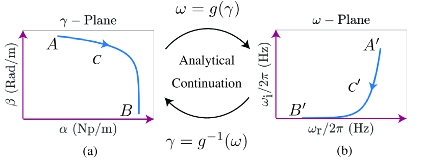
Figure 2: Statement of the general mapping problem: find, for any electromagnetic structure (also without analytical solution), the complex function $\omega=g(\gamma)$ that maps complex points in the $\gamma$-plane to complex points in the $\omega$-plane, and its reciprocal counterpart $\gamma=g^{-1}(\omega)$ that maps complex points in the $\omega$-plane to complex points in the $\gamma$-plane. Here, the complex function $\omega=g(\gamma)$ maps the points along the path $C$ between the points $A$ and $B$ in the $\gamma$-plane to the points along the path $C^{\prime}$ between the points $A^{\prime}$ and $B^{\prime}$ in the $\omega$-plane while the complex function $\gamma=g^{-1}(\omega)$ performs the reverse mapping. The function $g(\cdot)$ will be shown to be unique, by virtue of the combined principles of analytical continuity and wave physicality (Sec. IV).

III Problems with Analytical Solutions

We consider here three problems having a known analytical solution, both to further precise the problematic of the mapping problem introduced in Sec. II and to establish analytical benchmarks for the validation in Sec. V of our general method, that will be presented in Sec. IV.

III-A Lossy Medium

Let us first assume the relatively simple problem of an unbounded lossy medium [15]. The wave functions of this problem, for instance $\psi=\mathcal{E}_{z}(x,t)$, satisfy the Helmholtz wave equation

$$\frac{\partial^{2}\psi}{\partial t^{2}}-\frac{1}{\mu\epsilon}\frac{\partial^{2}\psi}{\partial x^{2}}+\frac{\sigma}{\epsilon}\frac{\partial\psi}{\partial t}=0,$$ (6)

where $\epsilon$, $\mu$ and $\sigma$ are respectively the permittivity, the permeability and the conductivity of the medium. A solution to (6) is

$$\mathcal{E}_{z}(x,t) =\text{e}^{-\alpha x}\cos({\omega_{\text{r}}t-\beta x)}$$

$$=\Re\{\text{e}^{-\gamma x}\text{e}^{j\omega_{\text{r}}t}\},$$ (7)

where $\gamma=\alpha+j\beta$ is the complex propagation constant. Substituting (III-A) in (6) results into

$$\gamma(\omega_{\text{r}})=\pm j\frac{\omega_{\text{r}}}{\nu}\sqrt{1-j\frac{\sigma}{\omega_{\text{r}}\epsilon}},$$ (8)

where $\nu=1/\sqrt{\mu\epsilon}$ is the speed of the wave in the medium. Equation (8) provides the complex propagation constant, $\gamma$, corresponding to the real frequency, $\omega_{\text{r}}$, for the medium parameters $\epsilon$, $\mu$ and $\sigma$.

Alternatively, fixing the magnitude of the wave in space, i.e., setting $\alpha=0$, and letting the phase vary, i.e., $\beta\neq 0$, leads to

$$\mathcal{E}_{z}(x,t) =\Re\{\text{e}^{-j\beta x}\text{e}^{j\omega t}\}$$

$$=\text{e}^{-\omega_{\text{i}}t}\cos({\omega_{\text{r}}t-\beta x)},$$ (9)

with complex frequency $\omega=\omega_{\text{r}}+j\omega_{\text{i}}$, which is also solution to (6). Substituting (III-A) in (6) results into

$$\beta=\pm\frac{\omega}{\nu}\sqrt{1-j\frac{\sigma}{\omega\epsilon}},$$ (10)

which is exactly Eq. (8) except that $\gamma$ and $\omega_{\text{r}}$ are replaced by $j\beta$ and $\omega$, respectively. Solving Eq. (10) for $\omega$ yields

$$\omega(\beta)=\pm\sqrt{\nu^{2}\beta^{2}-\frac{\sigma^{2}}{4\epsilon^{2}}}+j\frac{\sigma}{2\epsilon}.$$ (11)

Equation (11) provides the complex frequency $\omega$, given the phase constant $\beta$ and the medium parameters $\epsilon$, $\mu$ and $\sigma$.

Figure 3(a) shows $\gamma=j\beta$ in the $\gamma$-plane while Fig. 3(b) shows its map in the $\omega$-plane given by the Eq. (11). Conversely, Fig. 3(b) shows the $\omega=\omega_{\text{r}}$ in the $\omega$-plane while Fig. 3(a) shows its map in the $\gamma$-plane given by the Eq. (8).

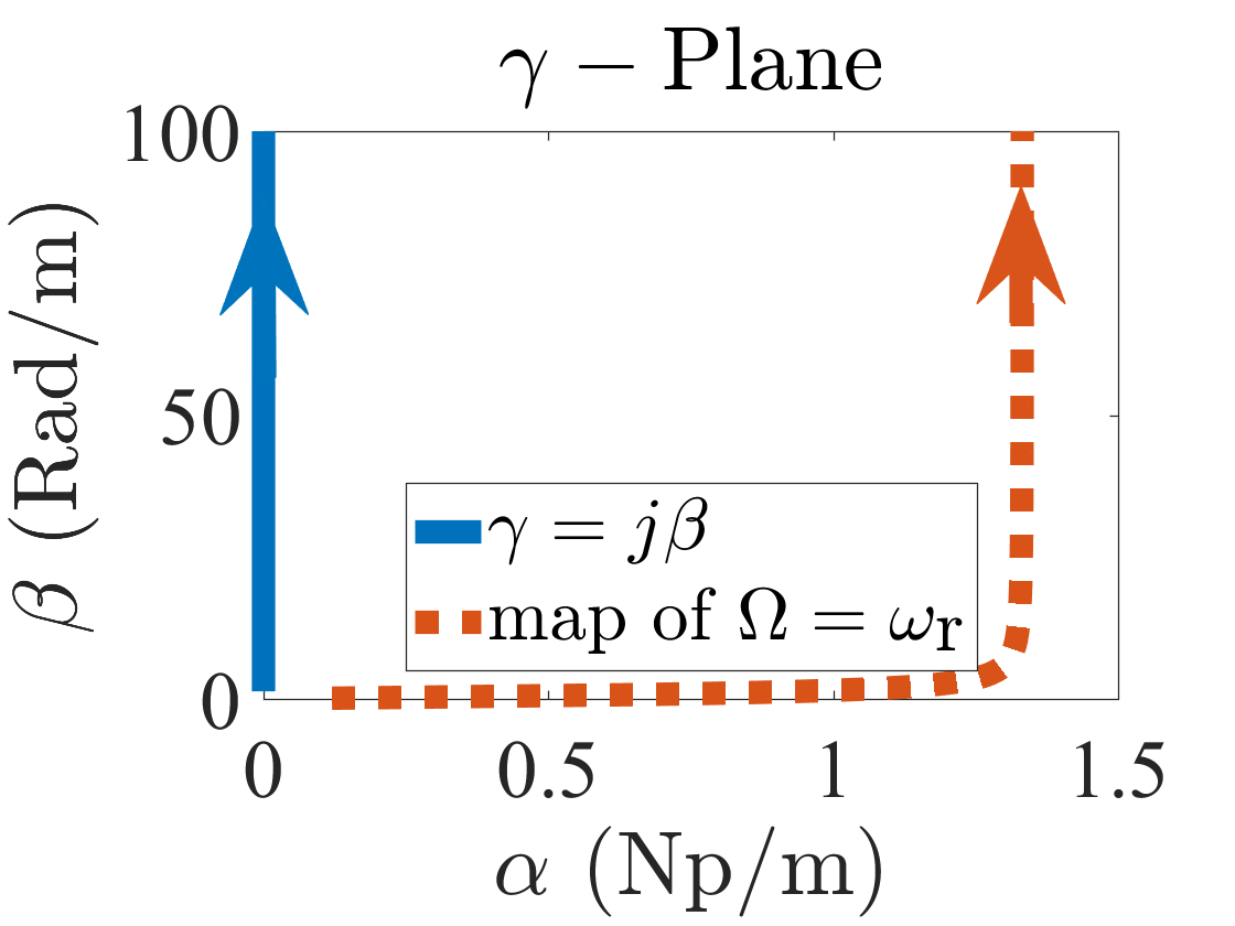
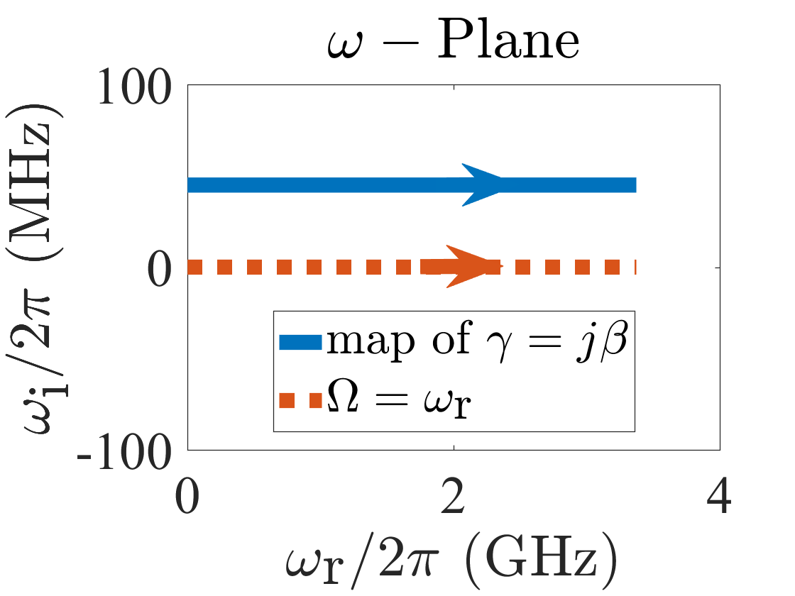
Figure 3: Mapping for an unbounded lossy medium with relative permittivity $\epsilon_{\text{r}}=2.2$ and conductivity $\sigma=0.01~{}\textrm{S/m}$. (a) $\gamma$-plane, with $\omega=\omega_{\text{r}}$ mapping using Eq. (8). (b) $\omega$-plane, with $\gamma=j\beta$ mapping using Eq. (11).

A couple of important observations are in order.

1. According to Eq. (11), the real part of the complex frequency $\omega_{\text{r}}=\pm\sqrt{\nu^{2}\beta^{2}-{\sigma^{2}}/{4\epsilon^{2}}}$ is approximately $\omega_{\text{r}}\approx\pm\nu\beta$ in a low-loss dielectric medium, where $\sigma/2\epsilon\ll\nu\beta$, and the imaginary part of $\omega$ is then a positive constant $\omega_{\text{i}}={\sigma}/{2\epsilon}$.

2. According to Eq. (8) and choosing the positive sign for the forward propagating waves, the real part of $\gamma$ is approximately constant $\alpha\approx\sigma/2\epsilon\nu$ and the imaginary part of $\gamma$ is approximately $\beta\approx\omega_{\text{r}}/\nu$ for a low loss medium where $\sigma/\omega_{\text{r}}\epsilon\ll 1$.

The equations (III-A) and (III-A) are both solutions of the Helmholtz equation (6), but have different boundary conditions. Equation (III-A) is the solution for the driven-mode regime while Eq. (III-A) is the solution for the eigen-mode regime. If the eigen-mode regime would accept magnitude differences at the boundaries in addition to the phase differences, then the general representation

$$\psi(x,t)=\Re\{\text{e}^{-\gamma x}\text{e}^{j\omega t}\},$$ (12)

would lead to a solution of the wave equation (6) with $\gamma$ and $\omega$ both complex.

Inserting Eq. (12) into (6) results in the complex dispersion relation

$$\omega^{2}+\frac{1}{\mu\epsilon}\gamma^{2}-j\frac{\sigma}{\epsilon}\omega=0,$$ (13)

which reduces to Eq. (8) if $\omega=\omega_{\text{r}}$ and to Eq. (11) if $\gamma=j\beta$. Equation (13) provides the most general mapping function $g$ from the $\gamma$-plane into the $\omega$-plane, given by

$$\omega =g(\gamma)$$

$$=j\left(\frac{\sigma}{2\epsilon}\pm\sqrt{\nu^{2}\gamma^{2}+\frac{\sigma^{2}}{4\epsilon^{2}}}\right),$$ (14a)

while, inversely, the mapping function $$g^{-1} \omega \gamma$$ from the -plane into the -plane, given by

$$\gamma =g^{-1}(\omega)$$

$$=\pm j\frac{\omega}{\nu}\sqrt{1-j\frac{\sigma}{\omega\epsilon}}.$$ (14b)

III-B Dielectric-filled Metallic Waveguide

Second, we consider the rectangular metallic waveguide filled with a lossy dielectric material [16]. The wave functions of this problem, for instance $\psi=\mathcal{H}_{x}(x,t)$ or $\psi=\mathcal{E}_{x}(x,t)$, satisfy the Helmholtz wave equation

$${\mu\epsilon}\frac{\partial^{2}\psi}{\partial t^{2}}-\frac{\partial^{2}\psi}{\partial x^{2}}+\kappa_{m,n}^{2}\psi+{\mu\sigma}\frac{\partial\psi}{\partial t}=0,$$ (15)

where $\kappa_{m,n}=\sqrt{\left({m\pi}/{a}\right)^{2}+\left({n\pi}/{b}\right)^{2}}$, with $a$ and $b$ representing the dimensions of the rectangular cross section of the waveguide, and ($m$,$n$) denotes the mode number.

Inserting Eq. (III-A) in (15) yields

$$\gamma(\omega_{\text{r}})=\pm j\frac{\omega_{\text{r}}}{\nu}\sqrt{1-\left(\frac{\nu\kappa_{m,n}}{\omega_{\text{r}}}\right)^{2}-j\frac{\sigma}{\omega_{\text{r}}\epsilon}},$$ (16)

while inserting Eq. (III-A) in (15) yields

$$\omega(\beta)=\pm\sqrt{\nu^{2}\left(\beta^{2}+\kappa_{m,n}^{2}\right)-\frac{\sigma^{2}}{4\epsilon^{2}}}+j\frac{\sigma}{2\epsilon}.$$ (17)

Figure 4(a) shows $\gamma=j\beta$ in the $\gamma$-plane while Fig. 4(b) shows its map in the $\omega$-plane given by the Eq. (17) and reversely, Fig. 4(b) shows the $\omega=\omega_{\text{r}}$ in the $\omega$-plane and Fig. 4(a) shows its map in the $\gamma$-plane given by the Eq. (16) for the $\text{TE}_{10}$ mode where $m=1$ and $n=0$ (i.e., $\kappa_{m,n}=\pi/a$).

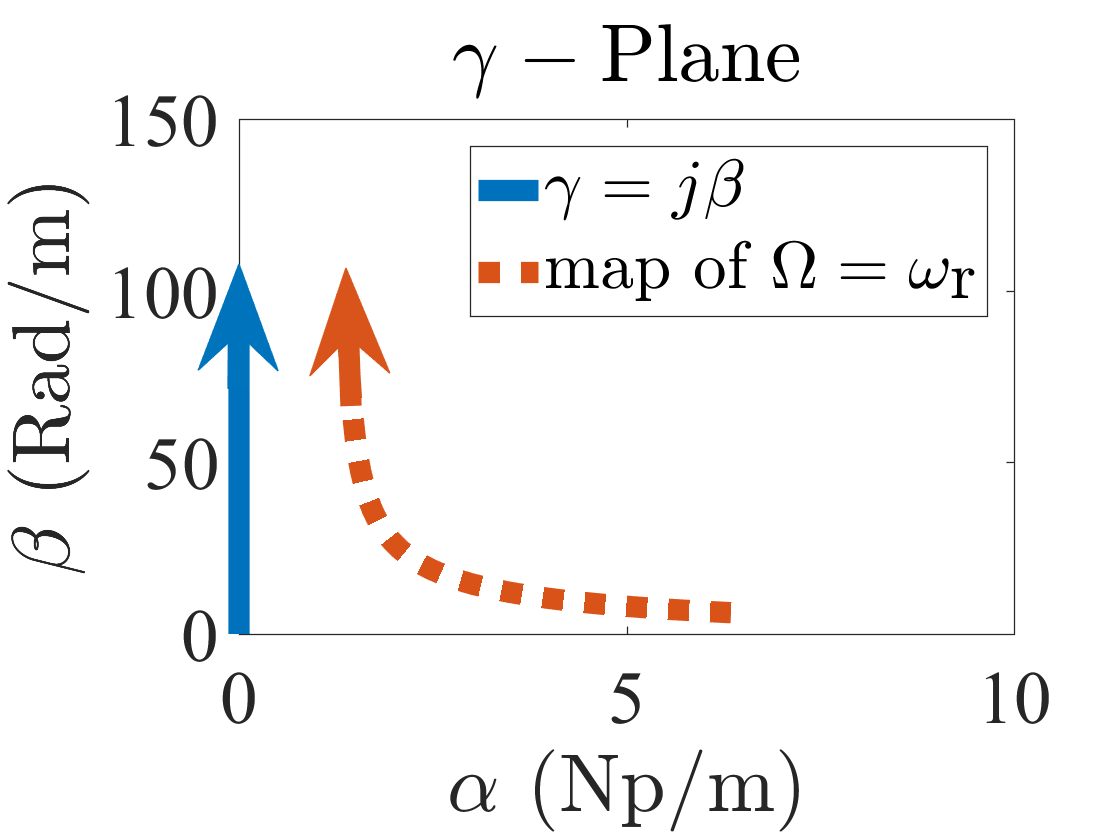
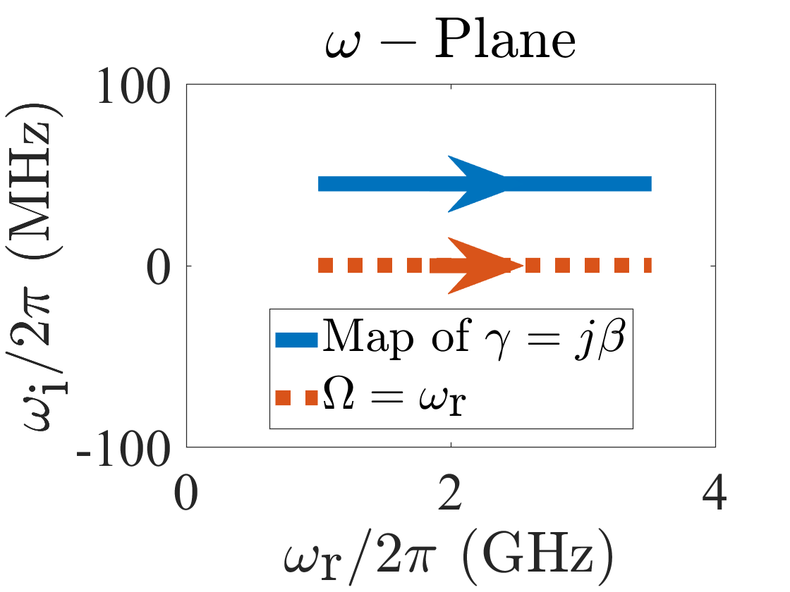
Figure 4: Mapping for a rectangular metallic waveguide filled with a lossy dielectric material with $\epsilon_{\text{r}}=2.2$ and $\sigma=0.01~{}\textrm{S/m}$ of width $a=\lambda_{\text{g}}/2$ where $\lambda_{\textrm{g}}=\lambda_{0}/\sqrt{\epsilon_{\text{r}}}$ is the wavelength in the dielectric medium and $\lambda_{0}=30~{}\text{cm}$, corresponding to the cut-off frequency of 1 GHz for the $\text{TE}_{10}$ mode. (a) $\gamma$-plane, with $\omega=\omega_{\text{r}}$ mapping using Eq. (16). (b) $\omega$-plane, with $\gamma=j\beta$ mapping using Eq. (17).

A couple of important observations are in order.

1. According to Eq. (17), the real part of the complex frequency $\omega_{\text{r}}=\pm\sqrt{\nu^{2}\tilde{\beta}^{2}-{\sigma^{2}}/{4\epsilon^{2}}}$ (where $\tilde{\beta}^{2}={\beta^{2}+\kappa_{m,n}^{2}}$) is approximately $\omega_{\text{r}}\approx\pm\nu\tilde{\beta}$ for a low-loss medium where $\sigma/2\epsilon\ll\nu\tilde{\beta}$, and the imaginary part of $\omega$ is then a positive constant $\omega_{\text{i}}={\sigma}/{2\epsilon}$.

2. According to Eq. (16), and choosing the positive sign for the forward propagating waves, the real part of $\gamma$ is approximately $\alpha\approx(\omega_{\text{r}}/\tilde{\omega_{\text{r}}})\sigma/2\epsilon\nu$ (where $\tilde{\omega_{\text{r}}}=\sqrt{\omega_{\text{r}}^{2}-\nu^{2}\kappa_{m,n}^{2}}$) and the imaginary part of $\gamma$ is approximately $\beta\approx\tilde{\omega_{\text{r}}}/\nu$ for a low-loss medium where $\omega_{\text{r}}\sigma/\tilde{\omega_{\text{r}}}^{2}\epsilon\ll 1$.

Equations (16) and (17) are solutions of the wave equation (15). Inserting the general wave representation (12) into (15), we obtain the following general dispersion equation

$$\omega^{2}+\frac{1}{\mu\epsilon}(\gamma^{2}-\kappa_{m,n}^{2})-j\frac{\sigma}{\epsilon}\omega=0,$$ (18)

which reduces to Eq. (16) if $\omega=\omega_{\text{r}}$ and to Eq. (17) if $\gamma=j\beta$. Equation (18) results in the mapping function $g$ from the $\gamma$-plane into the $\omega$-plane, given by

$$\omega =g(\gamma)$$

$$=j\left(\frac{\sigma}{2\epsilon}\pm\sqrt{\nu^{2}(\gamma^{2}-\kappa_{m,n}^{2})+\frac{\sigma^{2}}{4\epsilon^{2}}}\right),$$ (19a)

and inversely the mapping function $$g^{-1} \omega \gamma$$ from the -plane into the -plane, given by

$$\gamma =g^{-1}(\omega)$$

$$=\pm j\frac{\omega}{\nu}\sqrt{1-\left(\frac{\nu\kappa_{m,n}}{\omega}\right)^{2}-j\frac{\sigma}{\omega\epsilon}}.$$ (19b)

III-C Periodically-loaded Transmission Line

Finally, let us consider a loaded transverse electromagnetic (TEM) transmission line (TL) that is periodically loaded by shunt lossy capacitive loads with periodicity $p$ [5].

The voltage or current functions, $\psi=\mathcal{V}(x,t)$ and $\psi=\mathcal{I}(x,t)$, of such a TL satisfy the wave equation

$${LC}\frac{\partial^{2}\psi}{\partial t^{2}}-\frac{\partial^{2}\psi}{\partial x^{2}}+RG\psi+\left(LG+RC\right)\frac{\partial\psi}{\partial t}=0,$$ (20)

where $R$ ($\omega$/m), $G$ (S/m), $L$ (H/m) and $C$ (F/m) are the per-unit-length series resistance, shunt conductance, series inductance and shunt capacitance, respectively. On the other hand, the voltage $V(t)$ and current $I(t)$ for a shunt lossy capacitive load satisfy the equation

$$\tilde{C}\frac{dV}{dt}+\tilde{G}{V}=I,$$ (21)

where $\tilde{C}$ (F) and $\tilde{G}$ (S) are capacitance and conductance of the lumped load, respectively. Equations (20) and (21) both admit solutions of the form (III-A), (III-A) and (12).

The relation between the voltages and currents at either side of the $n^{\text{th}}$ unit cell is given by [5]

$$\begin{pmatrix}V_{n}\\ I_{n}\end{pmatrix}=\begin{pmatrix}A&B\\ C&D\end{pmatrix}\begin{pmatrix}V_{n+1}\\ I_{n+1}\end{pmatrix},$$ (22)

where $A$, $B$, $C$ and $D$ are the transmission matrix parameters of a cascaded load-free $p/2$-length TL, shunt admittance $Y$ and $p/2$-length unloaded TL. Equating the $ABCD$ matrix to that of a section of an equivalent TL with length $p$ and complex propagation constant $\gamma$ leads to (see [5], Sec. 8, page 383)

$$\gamma(\omega_{\text{r}})=\frac{1}{p}\cosh^{-1}\left[\cos\left(\frac{\omega_{\text{r}}}{\nu}p\right)-\frac{b}{2}\sin\left(\frac{\omega_{\text{r}}}{\nu}p\right)\right],$$ (23)

where $b=-jYZ_{0}$ and $Z_{0}$ is the characteristic impedance of the unloaded TL. The function $\gamma(\omega_{\text{r}})$ is periodic with periodicity $\nu\pi/p$ according to Eq. (23).

On the other hand, if we replace $\omega_{\text{r}}$ by the complex $\omega$ and the complex $\gamma$ by purely imaginary $j\beta$ in Eq. (23), we find the complex $\omega$ given by

$$\omega(\beta)=\frac{\nu}{p}\left(\cos^{-1}\left[\cos(\beta p)\cos\phi\right]-\phi\right),$$ (24a)

where

$$\phi=\tan^{-1}\left(\frac{b}{2}\right).$$ (24b)

The function $\omega(\beta)$ is periodic with periodicity $\pi/p$ according to Eq. (24).

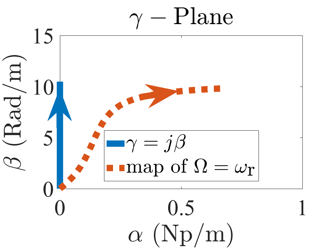
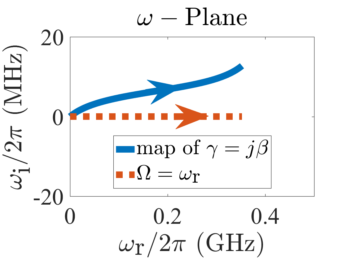
Figure 5: Mapping for a TL periodically loaded by lossy capacitive loads with normalized admittance $YZ_{0}=0.1+j$ and periodicity $p=30$ cm. (a) $\gamma$-plane, with $\omega=\omega_{\text{r}}$ mapping using Eq. (23). (b) $\omega$-plane, with $\gamma=j\beta$ mapping using Eq. (24). $\gamma$ is periodic with periodicity $j\pi/p\approx j10.5~{}(\text{Rad}/\text{m})$ and $\omega/2\pi$ is periodic with periodicity $\nu/2p\approx 0.5$ GHz.

Letting $\omega$ and $\gamma$ be both complex in Eq. (23), we obtain the general dispersion equation

$$\cosh\gamma p=\cos\left(\frac{\omega}{\nu}p\right)-\frac{b}{2}\sin\left(\frac{\omega}{\nu}p\right),$$ (25)

which reduces to Eq. (23) if $\omega=\omega_{\text{r}}$ and to Eq. (24) if $\gamma=j\beta$. Equation (25) provides the mapping function $g$ from the $\gamma$-plane into the $\omega$-plane,

$$\omega =g(\gamma)$$

$$=\frac{\nu}{p}\left(\cos^{-1}\left[\cosh(\gamma p)\cos\phi\right]-\phi\right).$$ (26a)

and inversely the mapping function $$g^{-1} \omega \gamma$$ from the -plane into the -plane,

$$\gamma =g^{-1}(\omega)$$

$$=\frac{1}{p}\cosh^{-1}\left[\cos\left(\frac{\omega}{\nu}p\right)-\frac{b}{2}\sin\left(\frac{\omega}{\nu}p\right)\right].$$ (26b)

IV General Mapping using Analytic Continuation

IV-A Motivation

Section III described the complex frequency mapping of some canonical problems that admit analytical solutions, namely an unbounded lossy medium, a dielectric-filled rectangular WG and a periodically-loaded TL. In these cases, we could obtain closed-form expressions for the mapping functions – $\gamma(\omega_{\text{r}})$, $\omega(\beta)$, $\omega=g(\gamma)$ and $\gamma=g^{-1}(\omega)$ – from the wave equations corresponding to the structure, specifically from Eqs. (6), (15) and (20) given the simplicity of the boundary conditions. Table I summarizes the mapping functions obtained for these problems with reference to the equation numbers in the text.

TABLE I: Mapping functions $\gamma(\omega_{\text{r}})$, $\omega(\beta)$, $\omega=g(\gamma)$ and $\gamma=g^{-1}(\omega)$ for the 3 examples in Sec. III.

Examples	lossy medium	rectangular WG	periodically-loaded TL
$\gamma(\omega_{\text{r}})$	$\pm j\frac{\omega_{\text{r}}}{\nu}\sqrt{1-j\frac{\sigma}{\omega_{\text{r}}\epsilon}}$	$\pm j\frac{\omega_{\text{r}}}{\nu}\sqrt{1-\left(\frac{\nu\kappa_{m,n}}{\omega_{\text{r}}}\right)^{2}-j\frac{\sigma}{\omega_{\text{r}}\epsilon}}$	$\frac{1}{p}\cosh^{-1}\left[\cos\left(\frac{\omega_{\text{r}}}{\nu}p\right)-\frac{b}{2}\sin\left(\frac{\omega_{\text{r}}}{\nu}p\right)\right]$
	Eq. (8)	Eq. (16)	Eq. (23)
$\omega(\beta)$	$\pm\sqrt{\nu^{2}\beta^{2}-\frac{\sigma^{2}}{4\epsilon^{2}}}+j\frac{\sigma}{2\epsilon}$	$\pm\sqrt{\nu^{2}\left(\beta^{2}+\kappa_{m,n}^{2}\right)-\frac{\sigma^{2}}{4\epsilon^{2}}}+j\frac{\sigma}{2\epsilon}$	$\frac{\nu}{p}\left(\cos^{-1}\left[\cos(\beta p)\cos\phi\right]-\phi\right)$
	Eq. (11)	Eq. (17)	Eq. (24)
$\omega=g(\gamma)$	$j\left(\frac{\sigma}{2\epsilon}\pm\sqrt{\nu^{2}\gamma^{2}+\frac{\sigma^{2}}{4\epsilon^{2}}}\right)$	$j\left(\frac{\sigma}{2\epsilon}\pm\sqrt{\nu^{2}(\gamma^{2}-\kappa_{m,n}^{2})+\frac{\sigma^{2}}{4\epsilon^{2}}}\right)$	$\frac{\nu}{p}\left(\cos^{-1}\left[\cosh(\gamma p)\cos\phi\right]-\phi\right)$
	Eq. (14)	Eq. (19)	Eq. (26)
$\gamma=g^{-1}(\omega)$	$\pm j\frac{\omega}{\nu}\sqrt{1-j\frac{\sigma}{\omega\epsilon}}$	$\pm j\frac{\omega}{\nu}\sqrt{1-\left(\frac{\nu\kappa_{m,n}}{\omega}\right)^{2}-j\frac{\sigma}{\omega\epsilon}}$	$\frac{1}{p}\cosh^{-1}\left[\cos\left(\frac{\omega}{\nu}p\right)-\frac{b}{2}\sin\left(\frac{\omega}{\nu}p\right)\right]$
	Eq. (14)	Eq. (19)	Eq. (26)

The availability of closed-form expressions for the mapping functions, as in Tab. I, naturally represents an ideal situation, since such solutions are exact, insightful and straightforward. Unfortunately, most practical systems, such as for instance a well-designed LWA structures [17], are too complex to admit closed-form, and even analytic, solutions. The analysis of such systems require full-wave simulations, which deliver purely numerical solutions. An approach capable to handle such problems is clearly needed.

IV-B General Problem and Resolution Procedure

Specifically, a general method is needed to map the numerical complex temporal frequencies of eigen-mode simulations into the corresponding complex spatial frequencies or, inversely, the numerical complex spatial frequencies of driven-mode simulations into the corresponding complex temporal frequencies. For this purpose, one has to find a generic function $g(\cdot)$, such that $\omega=g(\gamma)$ along the line $\gamma=j\beta$ of the complex $\gamma$ plane (eigen-mode computation) and $\gamma=g^{-1}(\omega)$ along the line $\omega=\omega_{\text{r}}$ of the complex $\omega$ plane (driven-mode computation).

We shall solve the problem by using the following four-step procedure:

1. Run a full-wave eigen-mode simulation or a driven-mode simulation of the problem to address so as to compute the data $\omega(\beta)=\omega_{\text{r}}(\beta)+j\omega_{\text{i}}(\beta)$ or $\gamma(\omega_{\text{r}})=\alpha(\omega_{\text{r}})+j\beta(\omega_{\text{r}})$, and record the numerical results, $[\beta,\omega_{\text{r}},\omega_{\text{i}}]$ or $[\omega_{\text{r}},\beta,\alpha]$, respectively.

2. Express the complex mapping function $g(\cdot)$ or $g^{-1}(\cdot)$ as polynomial expansion of $\beta$ around an analytic point $\beta_{0}$ or of $\omega_{\text{r}}$ around an analytic point $\omega_{\text{r},0}$, determine the expansion coefficients by fitting to the results of 1), and build the corresponding routine $g(\beta)$ or $g^{-1}(\omega_{\text{r}})$ in a calculator, respectively.

3. Substitute $\beta\rightarrow-j\gamma$ into the routine $g(\beta)$ or $\omega_{\text{r}}\rightarrow{j}\omega$ into the routine $g^{-1}(\omega_{\text{r}})$, respectively.

4. Find the complex roots $\gamma=\alpha+j\beta$ of the equation $\omega_{\text{r}}-g(\gamma)=0$ or $\omega=\omega_{\text{r}}+j\omega_{\text{i}}$ of the equation $j\beta-g^{-1}(\omega)=0$, respectively, which represent the sought after mapped solutions.

At this point the nature of the ‘function’ $g(\cdot)$ is still rather vague. However, we will be able to precise it shortly.

IV-C Analycity of the Solution

We are interested here in engineering problems, whose solutions obviously have a physical reality. Since the mathematical complex functions that describe physical problems are necessarily analytic [18], we can assert that the function $g(\cdot)$ must be analytic. We can then leverage the properties of analytic functions to assist us in characterizing $g(\cdot)$.

IV-D Theorem of Analytic Continuation

The most useful property of analytic functions toward the resolution of our problem is the property of analytic continuation. The theorem of analytic continuation states the following [19] (Sec. 27, page 84): A function that is analytic in a domain D is uniquely determined over D by its values in that domain or along any line segment contained in it.

Since we typically know the function only along line segments (Sec. IV-B), rather than in complete domains of analycity, the second part of the theorem, seems particularly convenient to us. We shall therefore focus on the statement: A function that is analytic in a domain D is uniquely determined over D by its values along any line segment contained in it. In other words, if an analytic function is known over a line segment of its analytic region, it is known everywhere, since this function is unique across the entire domain of analycity of the function.

Let us illustrate this theorem with the example of Fig. 6, which depict a function $w=f(z)$ that maps the complex plane $z=x+jy$ into the complex plane $w=u+jv$. In this example, it is assumed that the mapping of the straight line $z=jy$ within D in Fig. 6(a) is known as the curve plotted in Fig. 6(b). If we can construct the function $f(\cdot)$, for instance expressed as a polynomial expansion, fitted to the data $[y,u,v]$, this function is unique over the entire domain of analycity, and can therefore be used to map any curve, $C$, in the $z$ plane, represented in Fig. 6(c), into its image in the $w$ plane, as illustrated in Fig. 6(d).

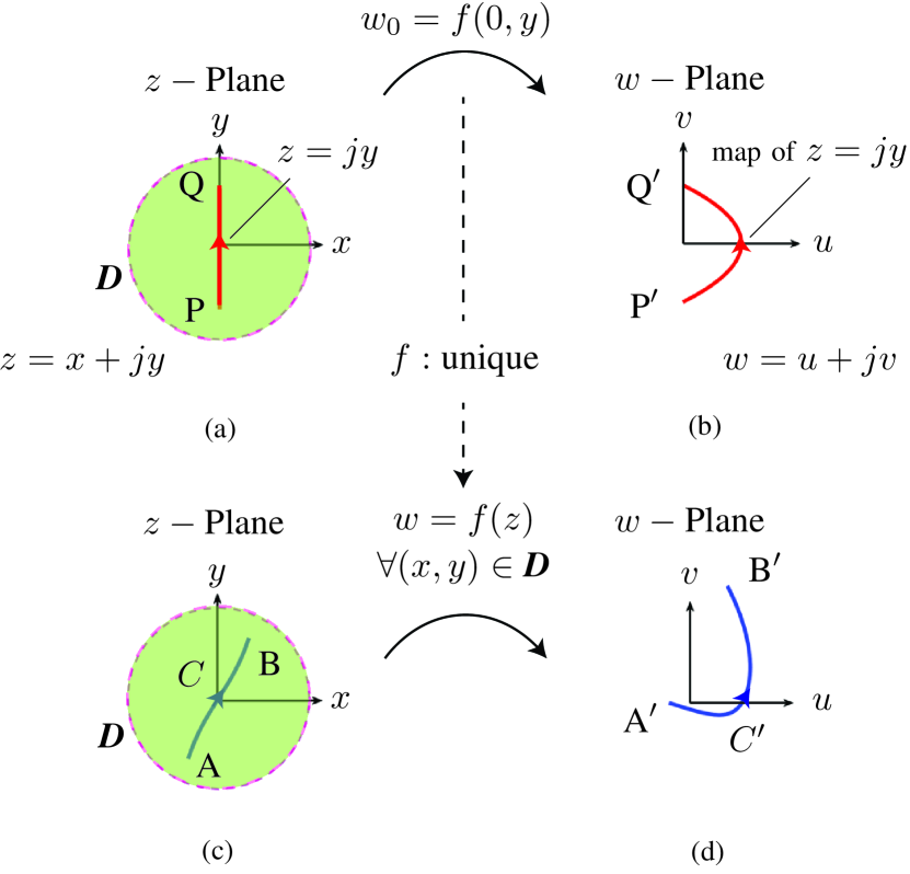
Figure 6: Illustration of the analytic continuation theorem. The green disk represents the domain of analycity of the function $f(\cdot)$. (a) Line $z=jy$ (or $x=0$) in the $z$-plane within the analyticity domain D. (b) Map of this line into the $w$-plane. (c) Arbitrary curve $C$ within the domain D of the $z$-plane. (d) Map of $C$ into the $w$-plane.

Let us further precise this explanation by considering a specific analytic mapping function $f(z)$ that is known in closed-form, as the mapping functions for the problems in Sec. III. Consider the function $f(z)=1+z+z^{2}$, for which the image of the line $z=jy$ (or $x=0$) in Fig. 6(a) is readily available as

$$w_{0}=f(0,y)=f(y)=(1-y^{2})+jy,$$ (27)

which corresponds in fact to the curve plotted in Fig. 6(b) as $u=1-y^{2}$ and $v=y$ versus the parameter $y$. Since we know, from the analytic continuation theorem, that the function $f(z)$ between the $z$ and $w$ planes is unique, we can replace its argument $(0,y)$ or $y$ in (27) by any complex value $z=x+jy$ and still find the correct mapping. In particular, we may substitute $y=-jz$, which yields

$$f(-jz) =f(z)=f(x,y)$$

$$=\left[1-(-jz)^{2}\right]+j(-jz)$$

$$=1+z+z^{2}$$

$$=(x^{2}-y^{2}+x+1)+j(2xy+y)$$

$$=u(x,y)+jv(x,y),$$ (28)

where the fourth equality indeed retrieves the original general analytic function $f(z)$ and the final result properly reduces to (27) for $z=(0,y)$. So, analytic continuity has allowed us to infer the general function $f(z)$, and hence the image of any curve $C$ of the $z$ plane in Fig. 6(c), as illustrated in Fig. 6(d)

Note that the mapping functions in Sec. III have not been found in this manner. Rather, these results were safely derived via the corresponding wave equations. However, we now know that this was an unnecessary complication. For instance, the general functions $\gamma=g^{-1}(\omega)$ of the fourth row in Tab. I can alternatively be found by simply substituting $\omega_{\text{r}}=\omega_{\text{r}}+j\omega_{\text{i}}$ in the first row! But we shall next consider the more practical situations of mapping functions without analytical solution.

IV-E General Mapping using Polynomial Expansion

We shall apply now the procedure described in Sec. IV-B, consolidated by the knowledge acquired in Sec. (IV-D) that the mapping function is unique, due to its analycity established in Sec. IV-C. For the sake of simplicity, we shall restrict our attention to the determination of the function $\omega=g(\beta)$ (eigen-mode analysis computation), the reciprocal function $\gamma=g^{-1}(\omega_{\text{r}})$ (driven-mode analysis computation) being obtainable in an analoguous manner. Thus,

1. First, we run an eigen-mode simulation of the problem at hand so as to compute the complex angular frequency $\omega(\beta)=\omega_{\text{r}}(\beta)+j\omega_{\text{i}}(\beta)$, and record the numerical result, i.e., $[\beta,\omega_{\text{r}},\omega_{\text{i}}]$.

2. Then, we build the function $g(\cdot)$ as the polynomial expansion

   $$\omega =g(\beta)$$

   $$=\omega_{\text{r}}(\beta)+j\omega_{\text{i}}(\beta)$$

   $$=\sum_{m=0}^{M}A_{m}(\beta-\beta_{0})^{m}+j\sum_{n=0}^{N}B_{n}(\beta-\beta_{0})^{n},$$ (29)

   where ($M$,$A_{m}$) and ($N$,$B_{n}$) are the best fitted-polynomial degrees and coefficients to the functions $[\beta,\omega_{\text{r}}]$ and $[\beta,\omega_{\text{i}}]$, respectively around the analytical point $\beta_{0}$.

3. Next, we replace the argument in the function $g(\beta)$ by $-j\gamma$ in the dispersion relation (2), which consequently transforms into

   $$\omega =g(\gamma)$$

   $$=\sum_{m=0}^{M}A_{m}(-j\gamma-\beta_{0})^{m}+j\sum_{n=0}^{N}B_{n}(-j\gamma-\beta_{0})^{n}.$$ (30)

   which relates $\omega$ and $\gamma$.

4. Finally, we compute the Max($M$,$N$) complex $\gamma=\alpha+j\beta$ roots of the equation

   $$\sum_{m=0}^{M}A_{m}(-j\gamma-\beta_{0})^{m}+j\sum_{n=0}^{N}B_{n}(-j\gamma-\beta_{0})^{n}-\omega_{\text{r}}=0,$$ (31)

   which provides the sought after map $\gamma(\omega_{\text{r}})=\alpha(\omega_{\text{r}})+j\beta(\omega_{\text{r}})$.

Note that an accurate estimation of the polynomial $\omega(\beta)$ in (2) requires a sufficient number and range of data points of complex $\omega$ versus $\beta$ values. For instance, finding the correct curve between $\text{P}^{\prime}$ and $\text{Q}^{\prime}$ in the $w$-plane in Fig. 6(b) (similarly in the $\omega$-plane) requires a sufficiently large number of points between the two points P and Q and a sufficiently extended range [P, Q] in the $z$-plane in Fig. 6(a) (similarly in the $\omega$-plane). Practically, a simple convergence analysis indicates when the number and range of points is sufficient.

Moreover, the point $\beta_{0}$ must be chosen in a region where the function $\omega(0+j\beta)$ is analytic, i.e., where the function $\omega$ and all its derivatives are continuous. Let us consider for example the case of the unbounded lossy medium, where $\omega(\gamma)$ is given by Eq. (14). In this case, $\gamma=j\sigma/2\epsilon\nu$ is the branch point and we may choose the branch cut $\beta<\sigma/2\epsilon\nu$, which requires $\beta_{0}>\sigma/2\epsilon\nu$. In the case of a medium with relatively low loss, $\beta_{0}$ may be safely set to approximately zero.

Finally, the proposed technique is not restricted to 1-D (periodic) structures; it can be readily generalized to 2-D and 3-D (periodic) structures. For example, for a 2-D periodic structure with periods $p_{1}$ and $p_{2}$ along the direct lattice vectors ${\textbf{a}}_{1}$ and ${\textbf{a}}_{2}$, we only need to run the eigen-mode analysis along the three segments of the irreducible Brillouin zone, formed by the reciprocal vectors ${\textbf{b}}_{1}$ and ${\textbf{b}}_{2}$, i.e., along the spectral paths $\Gamma-X$, $X-M$ and $M-\Gamma$ for a square lattice or $\Gamma-K$, $K-R$ and $R-\Gamma$ for a hexagonal lattice [8]. Once the complex frequencies, $\omega_{p}$, have been computed along the 3 $k_{p}$ paths ($p=1,2,3$), we can use the same algorithm as for the 1-D case to find $\omega_{p}=g(\gamma_{p})$, with $\omega$, $\beta$ and $\gamma$ respectively replaced by $\omega_{p}$, $k_{p}$ and $\gamma_{p}$.

V Validation and Illustrations

We shall now illustrate the general mapping technique established in Sec. IV for four practical examples and validate the results by either closed-form analytical solutions or driven-mode analysis full-wave results.

V-A Lossy Medium

First, we consider the lossy medium, analytically treated in Sec. III-A. From the complex frequency $\omega(\beta)$ data given by Eq. (11), we will see if the proposed mapping technique is consistent with the analytical solution, given by (8).

Figures 7(a) and (b) show the $\omega_{\text{r}}$ and $\omega_{\text{i}}$ data using Eq. (11) and their fitted curves/polynomials using Eq. (2) as functions of $\beta$, respectively. Figures 7(c) and (d) respectively show the $\alpha$ and $\beta$ estimated by the mapping technique Eq.(31) and the analytical formulation (8), and a close agreement between the two is observed.

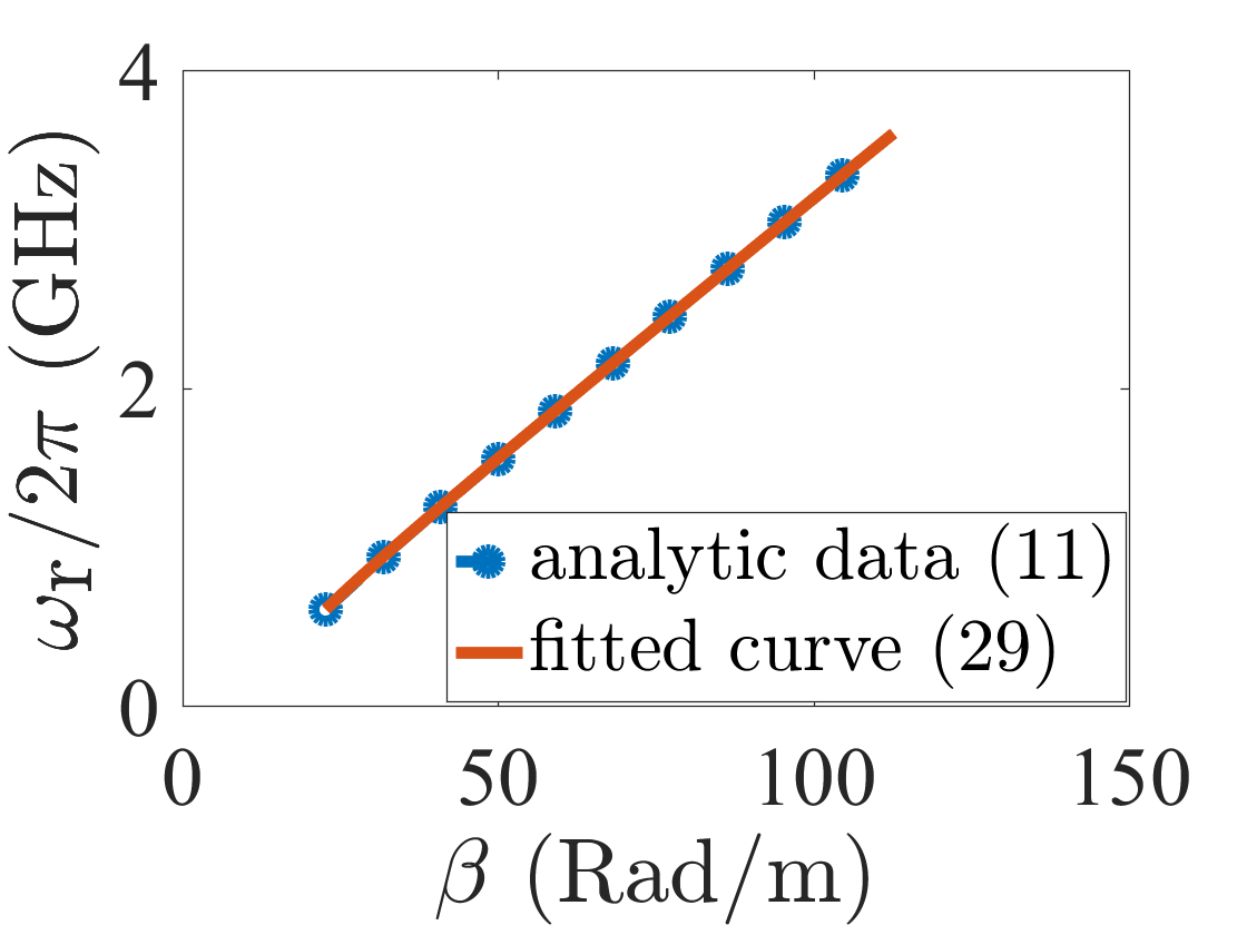
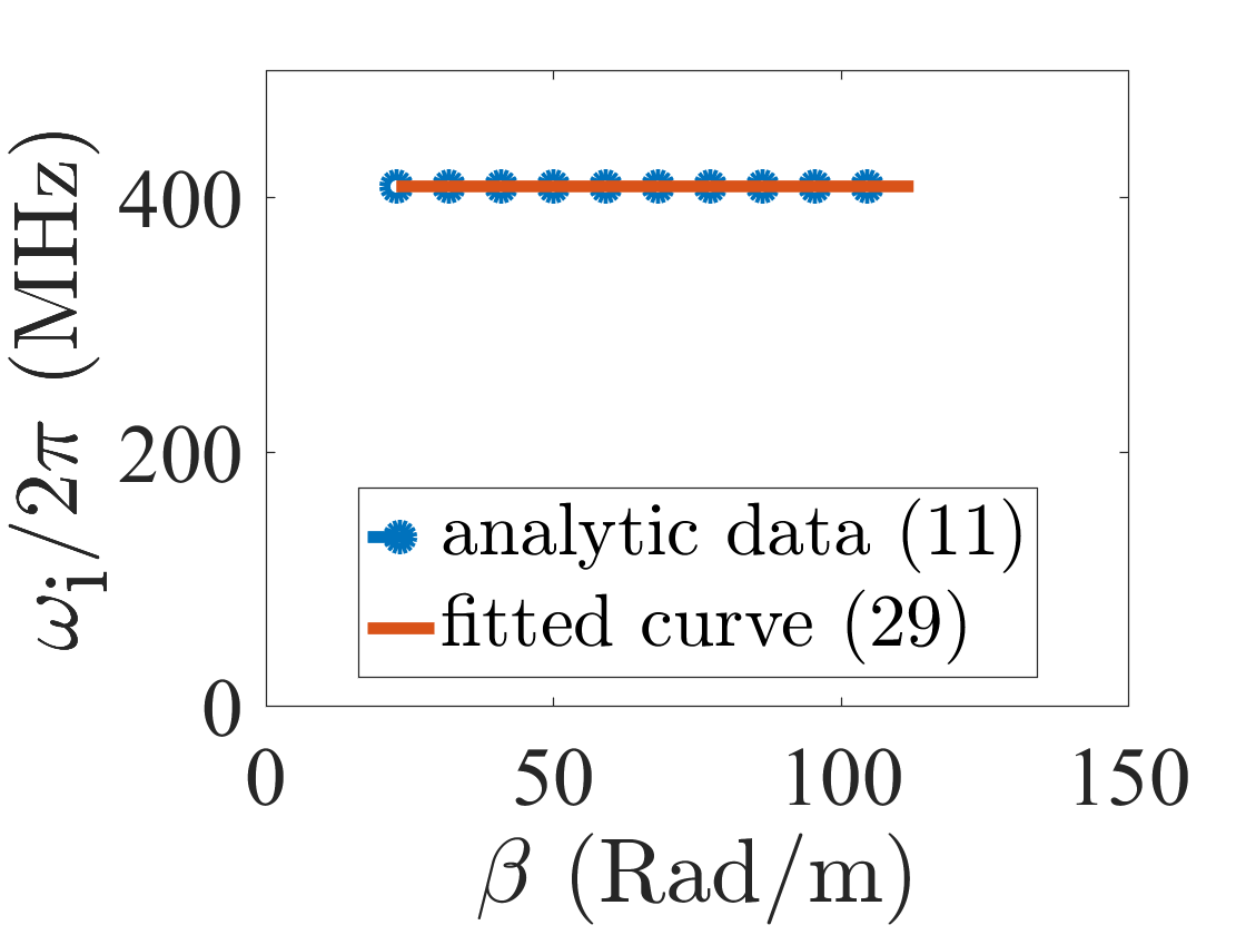
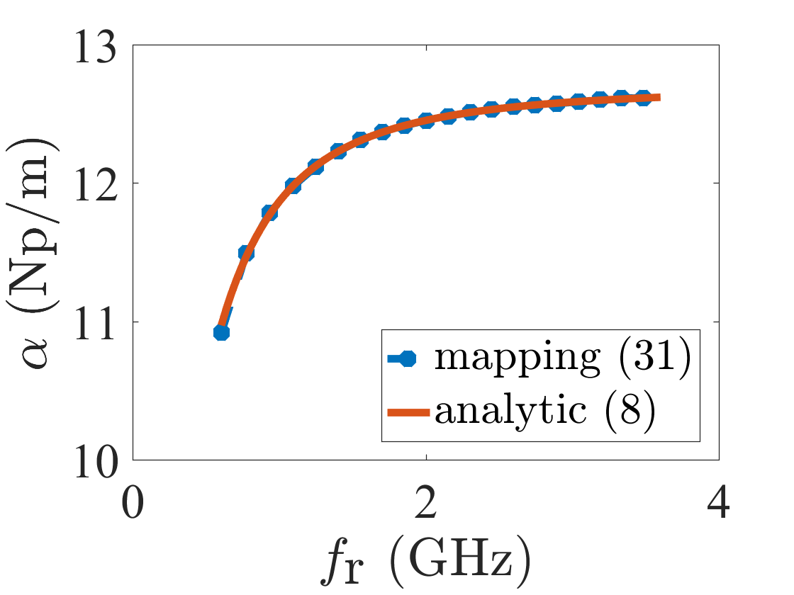
Figure 7: General mapping for an unbounded lossy dielectric medium with relative permittivity $\epsilon_{\text{r}}=2.2$ and conductivity $\sigma=0.1~{}\textrm{S/m}$. (a) $\omega_{\text{r}}(\beta)$. (b) $\omega_{\text{i}}(\beta)$. (c) $\alpha(f_{\text{r}})$. (d) $\beta(f_{\text{r}})$. The fitting polynomials of $\omega_{\text{r}}(\beta)$ and $\omega_{\text{i}}(\beta)$ have degrees 10 and 0, respectively, and $\beta_{0}$ is set $22.7>\sigma/2\epsilon\nu\approx 12.7$ rad/m.

V-B Dielectric-filled Metallic Waveguide

Second, we consider the rectangular waveguide in Sec.III-B, filled with a lossy dielectric. From the complex frequency $\omega(\beta)$ data given by Eq. (17), we will see if the proposed mapping technique is in agreement with the analytical solution, given by Eq. (16).

Figures 8(a) and (b) respectively show the $\omega_{\text{r}}$ and $\omega_{\text{i}}$ data using Eq. (17) and their fitted polynomials as functions of $\beta$. Figures 7(c) and (d) respectively show the $\alpha$ and $\beta$ estimated by the mapping technique and the analytical formulation (16) where perfect agreement between the two is observed.

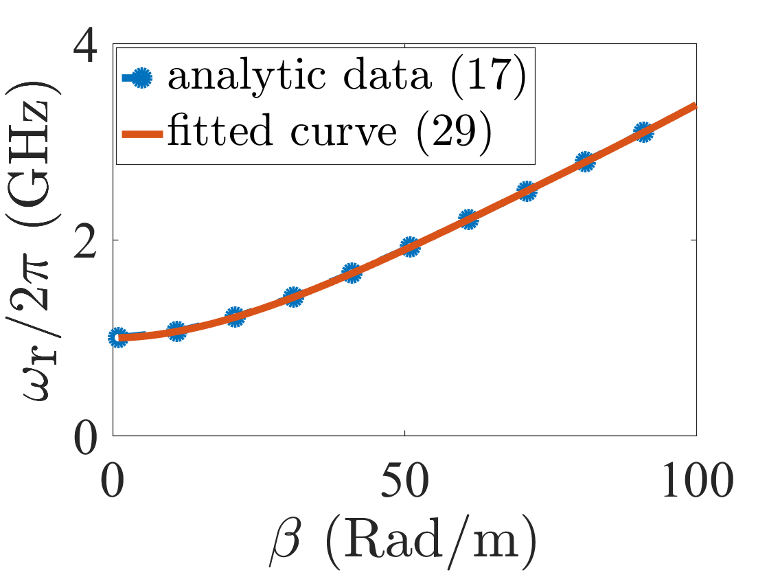
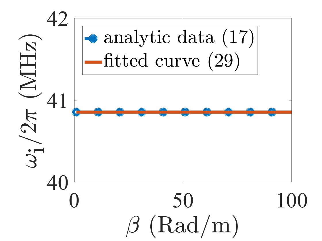
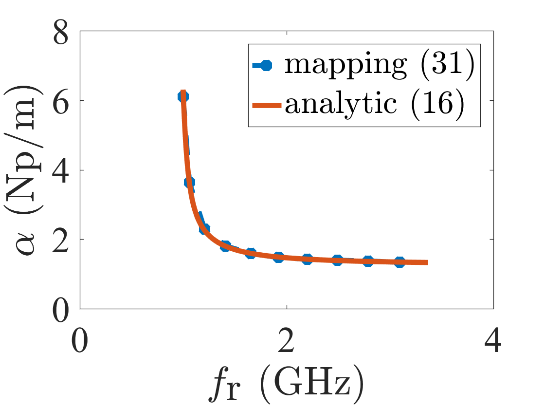
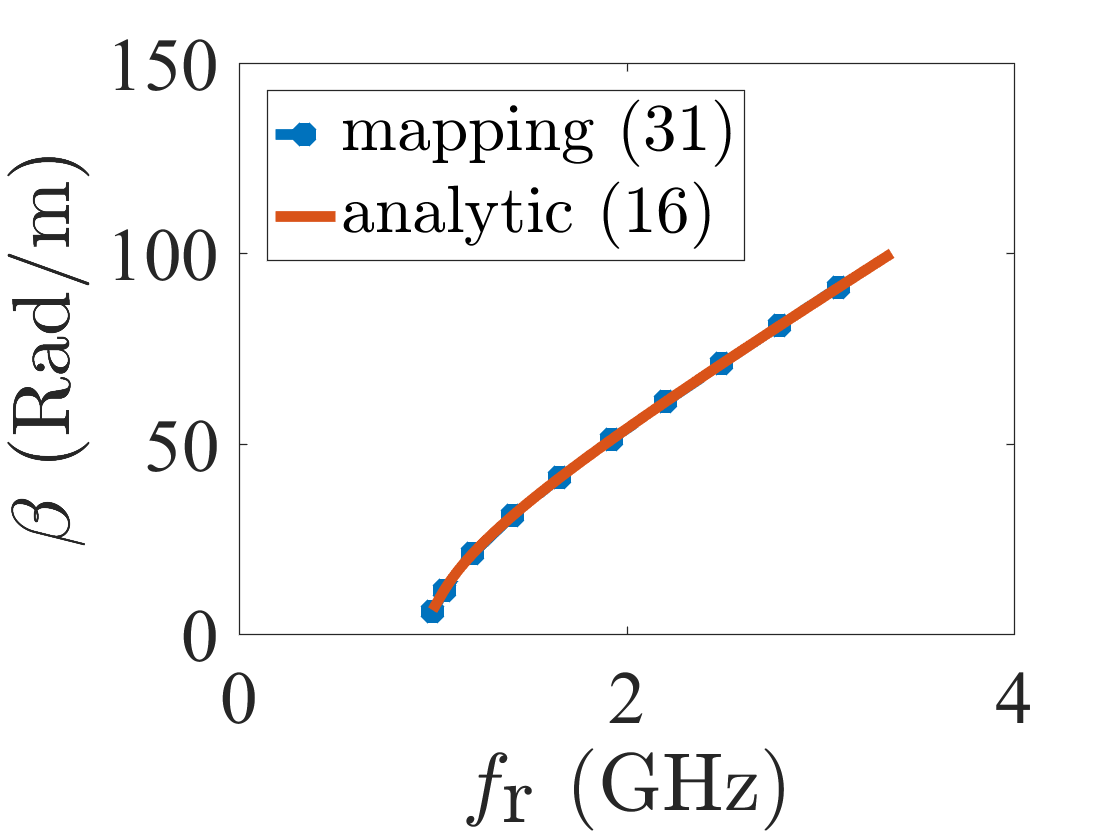
Figure 8: General mapping for a metallic rectangular waveguide filled with a lossy dielectric with $\epsilon_{\text{r}}=2.2$ and $\sigma=0.01~{}\textrm{S/m}$ and width $a=\lambda_{0}/2\sqrt{\epsilon_{\text{r}}}$ where $\lambda_{0}=30~{}\text{cm}$. (a) $\omega_{\text{r}}(\beta)$. (b) $\omega_{\text{i}}(\beta)$. (c) $\alpha(f_{\text{r}})$. (d) $\beta(f_{\text{r}})$. The fitting polynomials of $\omega_{\text{r}}(\beta)$ and $\omega_{\text{i}}(\beta)$ have degrees 4 and 0, respectively and $\beta_{0}=0$.

V-C 1-D Photonic Crystal

Figure 9 shows a 1-D periodic photonic crystal [8] whose dispersion relation is given by (Appendix A)

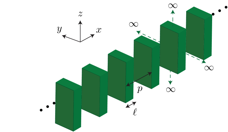
Figure 9: Photonic crystal consisting of lossy dielectric slabs with $\epsilon_{\text{r}}=4$ and $\sigma=0.01~{}\textrm{S/m}$, the periodicity $L=3~{}\text{cm}$ and thickness $\ell=L/2$.

$$\text{det}\begin{pmatrix}\text{e}^{-jk\ell}&~{}~{}\text{e}^{jk\ell}&-\text{e}^{-jk_{0}\ell}&-\text{e}^{jk_{0}\ell}\\ \text{e}^{-jk\ell}&-\text{e}^{jk\ell}&-\zeta\text{e}^{-jk_{0}\ell}&~{}~{}\zeta\text{e}^{jk_{0}\ell}\\ \text{e}^{-\gamma L}&~{}~{}\text{e}^{-\gamma L}&-\text{e}^{-jk_{0}L}&-\text{e}^{jk_{0}L}\\ \text{e}^{-\gamma L}&-\text{e}^{-\gamma L}&-\zeta\text{e}^{-jk_{0}L}&~{}~{}\zeta\text{e}^{jk_{0}L}\end{pmatrix}=0,$$ (32)

where $k=k_{0}\sqrt{\epsilon_{\text{rc}}}$, with $k_{0}=\omega/c$ ($c$: speed of light in vacuum), $\epsilon_{\text{rc}}={\epsilon_{\text{r}}-j\sigma/\omega\epsilon_{0}}$ and $\zeta=1/\sqrt{\epsilon_{\text{rc}}}$.

Equation (32) provides an analytical (but not closed-form) mapping function from the $\omega$-plane into the $\gamma$-plane and vise versa. Setting $\gamma=j\beta$ in Eq. (32) and finding the complex roots $\omega$ for which the determinant is zero yields the real and imaginary frequencies as functions of $\beta$. Figures 10(a) and (b) respectively show the $\omega_{\text{r}}$ and $\omega_{\text{i}}$ data and their fitted polynomials as functions of $\beta$ for the first 3 space harmonics.

Next, we apply the proposed mapping technique and compare the results with the analytical ones. The analytical results are again calculated by Eq. (32) in which we set the $\omega$ to be purely real $\omega_{\text{r}}$ and look for the complex roots $\gamma$ for which the determinant is zero. Figures 10(c) and (d) respectively show the $\alpha$ and $\beta$ estimated by the mapping technique and the analytical formulation based on (32) where again perfect agreements between the two are observed.

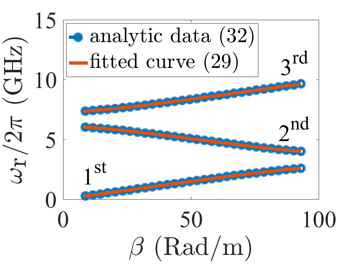
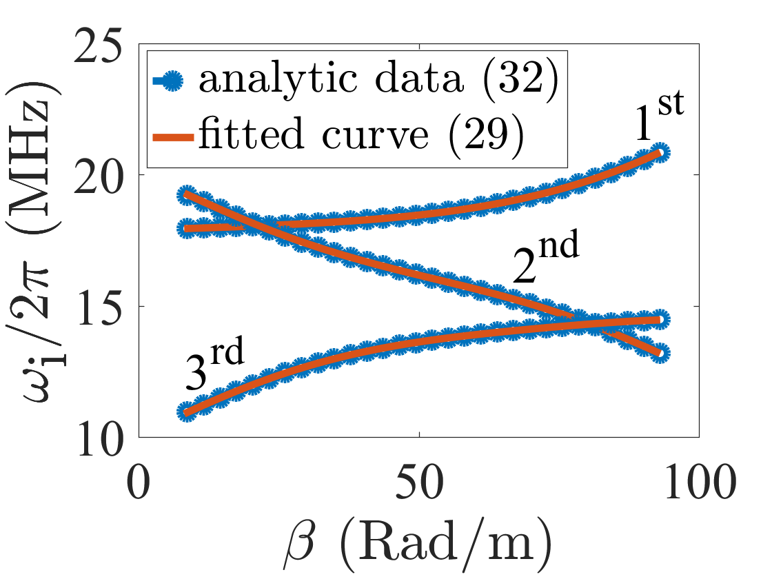
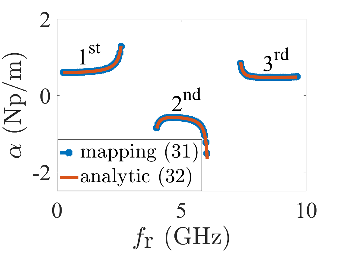
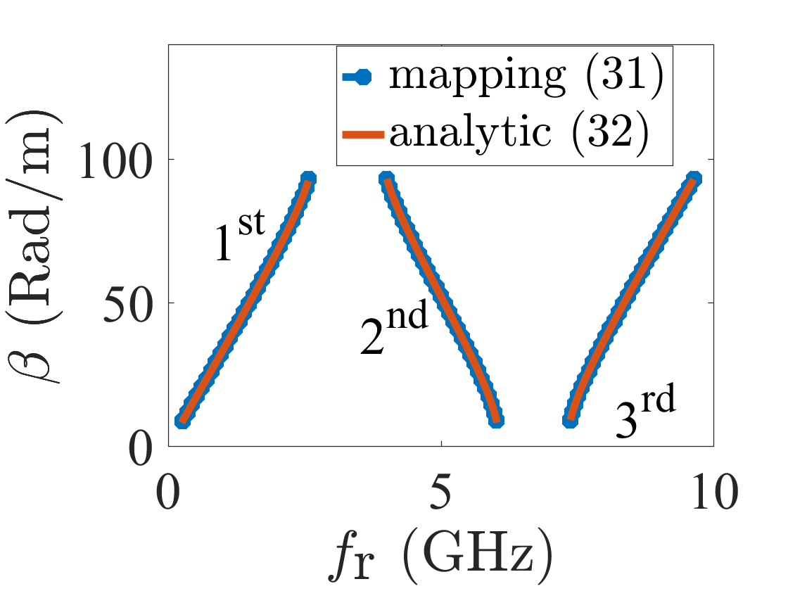
Figure 10: General mapping for the 1-D photonic crystal in Fig. 9 solutions for the first 3 space harmonics. (a) $\omega_{\text{r}}(\beta)$. (b) $\omega_{\text{i}}(\beta)$. (c) $\alpha(f_{\text{r}})$. (d) $\beta(f_{\text{r}})$. The polynomials of $\omega_{\text{r}}(\beta)$ and $\omega_{\text{i}}(\beta)$ both have the degree 5, and $\beta_{0}=0$.

V-D Leaky-Wave Antenna

Let us now consider the problem of a series-fed patch (SFP) periodic leaky-wave antenna (LWA), shown in Fig. 11, for which no analytical solution exist and full-wave numerical analysis is necessary [17]. Figures 11(a) and 11(b) show the unit cell setup of the eigen-mode analysis and the entire LWA 19-cell structure with the microstrip transmission line ports in the driven-mode analysis, respectively. As shown in Fig. 11(a), we place the unit cell inside a polygonal cylinder with assigned PBCs to the front and back faces and assigned surface impedance of $120\pi$ to the peripheral faces and a large enough radius to simulate radiation into free-space.

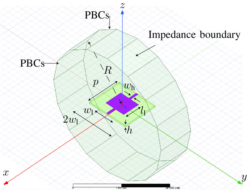
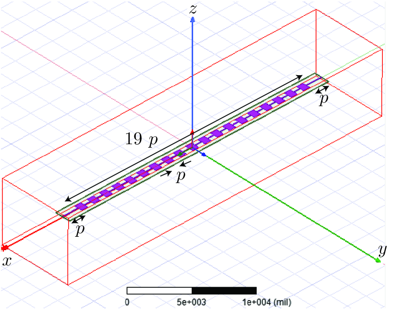
Figure 11: Periodic LWA problem. The antenna center frequency is set to $f_{\textrm{0}}=5.8~{}\textrm{GHZ}$ and the unit cell dimensions are $p=33.64~{}\text{mm}$, $l_{\text{l}}=p/2$, $w_{\text{l}}=20~{}\text{mm}$ and $w_{\text{h}}=2~{}\text{mm}$ [17]. The (lossless) substrate has a relative permittivity of $\epsilon_{\text{r}}=2.2$ and a height of $h=1.5~{}\text{mm}$. Ansys HFSS (a) eigen-mode and (b) driven-mode analysis setups. In the eigen-mode analysis the unit cell is placed within 16-segment polygonal cylinder with the radius $R=6~{}\text{cm}$ and assigned PBCs to the front and back faces and assigned surface impedance of $120\pi$ to the peripheral faces.

Figures 12(a) and (b) show the real and imaginary frequencies, $\omega_{\text{r}}$ and $\omega_{\text{i}}$ given by the eigen-mode analysis and their corresponding fitted polynomials as functions of $\beta$. We then apply the proposed mapping technique and compare the results with solutions of the driven-mode analysis of the Ansys HFSS. Figures 12(c) and (d) respectively show the $\alpha$ and $\beta$ estimated by the mapping technique and the Ansys HFSS driven-mode analysis where great agreement between the two is observed.

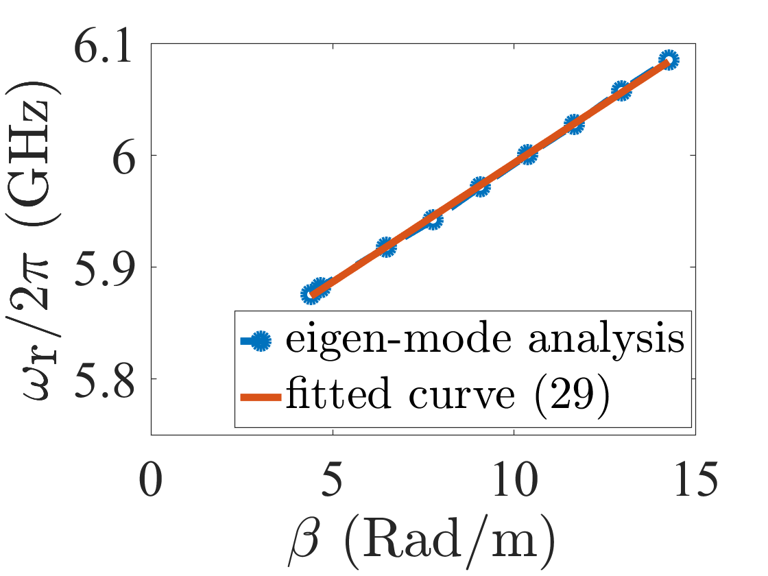
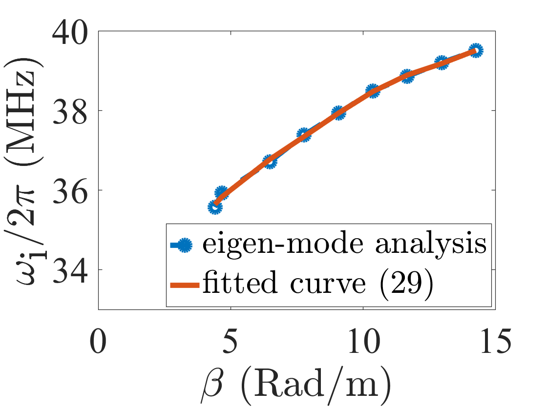
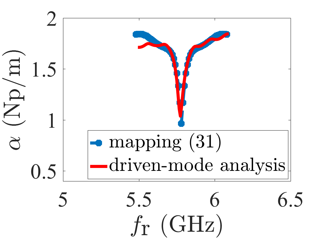
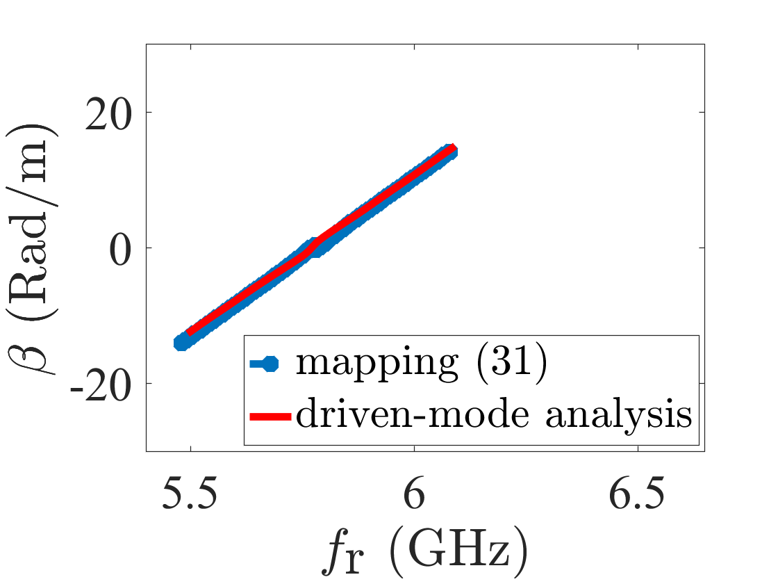
Figure 12: General mapping for the leaky-wave antenna in Fig. 11. (a) $\omega_{\text{r}}(\beta)$. (b) $\omega_{\text{i}}(\beta)$. (c) $\alpha(f_{\text{r}})$. (d) $\beta(f_{\text{r}})$. The polynomials of $\omega_{\text{r}}(\beta)$ and $\omega_{\text{i}}(\beta)$ have degrees 1 and 5, respectively, and $\beta_{0}=0$.

VI Conclusion

We introduced a new general method for mapping the complex spatial and temporal frequencies of an arbitrary electromagnetic structure, with and without analytical solution. The method is based on the analyticity of the physical mapping function and uses a fitted polynomial expansion to build this function, which is guaranteed by analytic continuity to be unique. This is a fundamental method, which is expected to find many applications in Electromagnetics.

Appendix A Derivation of Equation (32)

Let us assume a $z$-polarized plane wave propagating along the $x$ direction. The electromagnetic fields in the slab, ($E_{z}$, $H_{y}$), and in free-space, ($E_{z0}$, $H_{y0}$), regions of the periodic unit cell, are given in terms of forward and backward propagating waves, with ($A$,$B$) and ($C$,$D$) being unknown coefficients, as

$$\begin{pmatrix}E_{z}\\ H_{y}\end{pmatrix}=A\begin{pmatrix}1\\ {-1}/{\eta}\end{pmatrix}\text{e}^{-jkx}+B\begin{pmatrix}~{}~{}1\\ {1}/{\eta}\end{pmatrix}\text{e}^{jkx},$$ (A.1a)

$$\begin{pmatrix}E_{z0}\\ H_{y0}\end{pmatrix}=C\begin{pmatrix}1\\ {-1}/{\eta_{0}}\end{pmatrix}\text{e}^{-jk_{0}x}+D\begin{pmatrix}~{}~{}1\\ {1}/{\eta_{0}}\end{pmatrix}\text{e}^{jk_{0}x},$$ (A.1b)

where $\eta=\eta_{0}/\sqrt{\epsilon_{\text{rc}}}$, $\epsilon_{\text{rc}}={\epsilon_{\text{r}}-j\sigma/\omega\epsilon_{0}}$, $\eta_{0}=\sqrt{\mu_{0}/\epsilon_{0}}$, $k=k_{0}\sqrt{\epsilon_{\text{rc}}}$, $k_{0}=\omega/c$ and $c$ is the speed of light in vacuum.

Applying the continuity boundary conditions $(E_{z}=E_{z0})|_{x=\ell}$ and $(H_{y}=H_{y0})|_{x=\ell}$,

$$A\begin{pmatrix}1\\ -1/\eta\end{pmatrix}\text{e}^{-jk\ell}+B\begin{pmatrix}~{}~{}1\\ 1/\eta\end{pmatrix}\text{e}^{jk\ell}=$$

$$C\begin{pmatrix}1\\ -1/\eta_{0}\end{pmatrix}\text{e}^{-jk_{0}\ell}+D\begin{pmatrix}~{}~{}1\\ 1/\eta_{0}\end{pmatrix}\text{e}^{jk_{0}\ell}$$ (A.2a)

and next the periodic boundary conditions $$\text{e}^{-\gamma L}E_{z}|_{x=0}=E_{z0}|_{x=L} \text{e}^{-\gamma L}H_{y}|_{x=0}=H_{y0}|_{x=L}$$ and , given by

$$\text{e}^{-\gamma L}\left[A\begin{pmatrix}1\\ -1/\eta\end{pmatrix}+B\begin{pmatrix}~{}~{}1\\ 1/\eta\end{pmatrix}\right]=$$

$$C\begin{pmatrix}1\\ -1/\eta_{0}\end{pmatrix}\text{e}^{-jk_{0}L}+D\begin{pmatrix}~{}~{}1\\ 1/\eta_{0}\end{pmatrix}\text{e}^{jk_{0}L},$$ (A.2b)

results in the matrix equation

$$\begin{pmatrix}\text{e}^{-jk\ell}&~{}~{}\text{e}^{jk\ell}&-\text{e}^{-jk_{0}\ell}&-\text{e}^{jk_{0}\ell}\\ \text{e}^{-jk\ell}&-\text{e}^{jk\ell}&-\zeta\text{e}^{-jk_{0}\ell}&~{}~{}\zeta\text{e}^{jk_{0}\ell}\\ \text{e}^{-\gamma L}&~{}~{}\text{e}^{-\gamma L}&-\text{e}^{-jk_{0}L}&-\text{e}^{jk_{0}L}\\ \text{e}^{-\gamma L}&-\text{e}^{-\gamma L}&-\zeta\text{e}^{-jk_{0}L}&~{}~{}\zeta\text{e}^{jk_{0}L}\end{pmatrix}\begin{pmatrix}A\\ B\\ C\\ D\end{pmatrix}=\begin{pmatrix}0\\ 0\\ 0\\ 0\end{pmatrix},$$ (A.3)

where $\zeta=\eta/\eta_{0}=1/\sqrt{\epsilon_{\text{rc}}}$. For a non-trivial solution, the coefficient matrix must have a zero determinant, which results into Eq. (32).

References

- [1] J. C. Maxwell, “VIII. a dynamical theory of the electromagnetic field,” Philos. Trans. Royal Soc., no. 155, pp. 459–512, 1865.
- [2] J. D. Jackson, Classical Electrodynamics. John Wiley & Sons, 2007.
- [3] A. Ishimaru, Electromagnetic Wave Propagation, Radiation, and Scattering: from Fundamentals to Applications. John Wiley & Sons, 2017.
- [4] J. W. Goodman, Introduction to Fourier Optics, 4th ed. W. H. Freeman, Macmillan Learning, 2017.
- [5] D. M. Pozar, Microwave Engineering, 4th ed. John Wiley & Sons, 2011.
- [6] C. Caloz and Z.-L. Deck-Léger, “Spacetime metamaterials, part I: General concepts,” IEEE Trans. Antennas Propag., vol. 68, no. 2, pp. 1569–1582, Feb. 2020.
- [7] ——, “Spacetime metamaterials, part II: Theory and applications,” IEEE Trans. Antennas Propag., vol. 68, no. 2, pp. 1583–1598, Feb. 2020.
- [8] J. D. Joannopoulos, S. G. Johnson, J. N. Winn, and R. D. Meade, Photonic Crystals: Molding the Flow of Light, 2nd ed. Princeton University Press, 2008.
- [9] Z.-L. Deck-Léger, N. Chamanara, M. Skorobogatiy, M. G. Silveirinha, and C. Caloz, “Uniform-velocity spacetime crystals,” Adv. Photon., vol. 1, no. 5, pp. 056 002:1–26, Oct. 2019.
- [10] D. R. Jackson, C. Caloz, and T. Itoh, “Leaky-wave antennas,” Proc. IEEE, vol. 100, no. 7, pp. 2194–2206, 2012.
- [11] C. A. Desoer and E. S. Kuh, Basic Circuit Theory. McGraw-Hill, 1969.
- [12] C. Caloz and T. Itoh, Electromagnetic Metamaterials, Transmission Line Theory and Microwave Applications. Wiley - IEEE Press, 2006.
- [13] S. Otto, A. Al-Bassam, A. Rennings, K. Solbach, and C. Caloz, “Transversal asymmetry in periodic leaky-wave antennas for Bloch impedance and radiation efficiency equalization through broadside,” IEEE Trans. Antennas Propag., vol. 62, no. 10, pp. 5037–5054, Oct. 2014.
- [14] S. Otto, A. Rennings, K. Solbach, and C. Caloz, “Complex frequency versus complex propagation constant modeling and q-balancing in periodic structures,” in 2012 IEEE/MTT-S International Microwave Symposium Digest. IEEE, 2012, pp. 1–3.
- [15] W. Dyab, C. Caloz, and S. Otto, “Interpretation of complex frequencies in propagation problems,” in 2015 International Symposium on Antennas and Propagation (ISAP). IEEE, 2015, pp. 1–4.
- [16] D. J. King and S. Gupta, “Relation between complex propagation constant and complex eigenmodes in lossy traveling-wave structures,” in 2019 IEEE International Symposium on Antennas and Propagation and USNC-URSI Radio Science Meeting. IEEE, 2019, pp. 493–494.
- [17] S. Otto, A. Rennings, K. Solbach, and C. Caloz, “Transmission line modeling and asymptotic formulas for periodic leaky-wave antennas scanning through broadside,” IEEE Trans. Antennas Propag., vol. 59, no. 10, pp. 3695–3709, 2011.
- [18] P. M. Morse and H. Feshbach, Methods of Theoretical Physics. Vol. 1-2. McGraw-Hill, 1953.
- [19] J. W. Brown and R. V. Churchill, Complex Variables and Applications. Boston: McGraw-Hill Higher Education, 2009.