REGULARIZATION OF BACKWARD TIME-FRACTIONAL PARABOLIC EQUATIONS BY SOBOLEV-TYPE EQUATIONS

Dinh Nho Hào¹, Nguyen Van Duc², Nguyen Van Thang² and Nguyen Trung Thành³

¹ Hanoi Institute of Mathematics, VAST, 18 Hoang Quoc Viet, Hanoi, Vietnam
Email: hao@math.ac.vn
² Department of Mathematics, Vinh University, Vinh City, Vietnam,
Email: nguyenvanducdhv@gmail.com, nguyenvanthangk17@gmail.com
³Department of Mathematics, Rowan University, Glassboro, NJ, USA.
Email: nguyent@rowan.edu

Abstract: The problem of determining the initial condition from noisy final observations in time-fractional parabolic equations is considered. This problem is well-known to be ill-posed and it is regularized by backward Sobolev-type equations. Error estimates of Hölder type are obtained with a priori and a posteriori regularization parameter choice rules. The proposed regularization method results in a stable noniterative numerical scheme. The theoretical error estimates are confirmed by numerical tests for one- and two-dimensional equations.

Keywords: Backward time-fractional parabolic equations, Sobolev-type equations, numerical implementation.

1 Introduction

We consider the backward time-fractional parabolic equation:

$$\begin{cases}\dfrac{\partial^{\gamma}u}{\partial t^{\gamma}}+Au=0,\quad 0<t<T,\\ \|u(T)-f\|\leq\varepsilon,\end{cases}$$ (1.1)

where $\gamma\in(0,1)$,

$$\dfrac{\partial^{\gamma}u}{\partial t^{\gamma}}:=\dfrac{1}{\Gamma(1-\gamma)}\int_{0}^{t}(t-s)^{-\gamma}\dfrac{\partial u(\cdot,s)}{\partial s}ds,$$ (1.2)

is the Caputo derivative [11, 15], $\Gamma(\cdot)$ is Euler’s Gamma function, and $A:D(A)\subset\mathbb{H}\to\mathbb{H}$ is a self-adjoint closed operator on a Hilbert space $\mathbb{H}$. We assume that $-A$ generates a compact contraction semi-group $\{S(t)\}_{t\geq 0}$ on $\mathbb{H}$ and $A$ admits an orthonormal eigenbasis $\{\phi_{i}\}_{i\geq 1}$ in $\mathbb{H}$ associated with the eigenvalues $\{\lambda_{i}\}_{i\geq 1}$ such that

$$0<\lambda_{1}<\lambda_{2}<\ldots,\ \ \mbox{and}\ \ \lim\limits_{i\to+\infty}\lambda_{i}=+\infty.$$

In this work we denote the inner product and norm in $\mathbb{H}$ by $\left<\cdot,\cdot\right>$ and $\|\cdot\|$, respectively.

As an example of the operator $A$, consider the case $\mathbb{H}=L^{2}(\Omega)$, where $\Omega$ is a bounded domain in $\mathbb{R}^{d}$, $d\geq 1$, with sufficiently smooth boundary $\partial\Omega$. As usual, we denote by $H^{p}(\Omega)$ the Sobolev spaces. Denote by $H^{1}_{0}(\Omega)=\{u\in H^{1}(\Omega):u|_{\partial\Omega}=0\}.$ Then $A$ can be chosen as:

$$(Au)(x):=-\sum\limits_{i=1}^{d}\frac{\partial}{\partial x_{i}}\left(\sum\limits_{j=1}^{d}a_{ij}(x)\frac{\partial}{\partial x_{j}}u(x)\right)+c(x)u(x),x\in\Omega,$$

with $D(A)=H^{2}(\Omega)\cap H^{1}_{0}(\Omega).$ Here, we assume that $a_{ij}=a_{ji}\in C^{1}(\overline{\Omega}),i,j=1,\ldots,d;\ c\in C(\overline{\Omega}),\ c(x)\geq 0,\ \forall x\in\overline{\Omega}$; and $\sum_{i,j=1}^{d}a_{ij}(x)\xi_{i}\xi_{j}\geq\nu\sum_{i=1}^{d}\xi_{i}^{2},\ \forall x\in\overline{\Omega}$ for some $\nu>0$.

The backward problem (1.1) arises from several practical contexts, for example, in the determination of contaminant sources in underground fluid flow [8]. It is well-posed for $t>0$ and ill-posed for $t=0$, see [6]. Since the first work [12] devoted to the backward time-fractional diffusion equation, several papers on backward time-fractional parabolic equations have been published. For the mollification method, see [19, 26]; for the non-local boundary value problem method, see [6, 23, 24, 25]; and for Tikhonov regularization, we refer the reader to [1, 20, 21, 22]. In this paper we will regularize (1.1) by the backward Sobolev-type equations. Namely, we approximate the solution $u$ of (1.1) by the solution $v_{\alpha}$ of the following problem for the Sobolev-type equation:

$$\begin{cases}\dfrac{\partial^{\gamma}v_{\alpha}}{\partial t^{\gamma}}+\alpha A^{b}\dfrac{\partial^{\gamma}v_{\alpha}}{\partial t^{\gamma}}+Av_{\alpha}=0,~{}0<t<T,\\ v_{\alpha}(T)=f,\end{cases}$$ (1.3)

where $b$ is a real number such that $b\geq 1$, $\alpha>0$ is a regularization parameter, and operator $A^{b}$ is defined by

$$A^{b}v:=\sum\limits_{n=1}^{\infty}\lambda_{n}^{b}\left<v,\phi_{n}\right>\phi_{n},\quad\forall v\in D(A^{b}).$$ (1.4)

For this operator $A^{b}$, $I+\alpha A^{b}$ is invertible. Assuming that the fractional differentiation and $A^{b}$ are interchangeable, we can convert (1.3) into the following problem

$$\begin{cases}\dfrac{\partial^{\gamma}v_{\alpha}}{\partial t^{\gamma}}+A_{\alpha}v_{\alpha}=0,~{}0<t<T,\\ v_{\alpha}(T)=f,\end{cases}$$ (1.5)

where $A_{\alpha}=(I+\alpha A^{b})^{-1}A$.

Here, for $p>0$, we define

$$D(A^{p}):=\left\{\psi\in\mathbb{H}:\sum\limits_{n=1}^{\infty}\lambda_{n}^{2p}\left<\psi,\phi_{n}\right>^{2}<\infty\right\}$$

and the norm

$$\|\psi\|_{p}:=\left(\sum\limits_{n=1}^{\infty}\lambda_{n}^{2p}\left<\psi,\phi_{n}\right>^{2}\right)^{\frac{1}{2}},~{}\psi\in D(A^{p}).$$

For operator $A$ defined above, it has been shown that $D(A^{p})\subset H^{2p}(\Omega),\ p>0$, and $D(A^{\frac{1}{2}})=H_{0}^{1}(\Omega)$, see, e.g., [17].

The regularization method by Sobolev equations was first introduced by Gajewski and Zacharias for parabolic equations backward in time [5] (i.e., for the case $\gamma=1$). Since then, the method has been investigated in a number of works, see, e.g., [3, 4, 7, 9, 10, 13, 14, 16, 18]. However, there has been no error estimate in [5], [7], [18], and in the other related works, error estimates have been obtained only for a priori regularization parameter choice rules. A posteriori parameter choice rules have not been investigated yet.

To the best of our knowledge, the present work is the first one to use the Sobolev-type equations for regularizing the backward time-fractional parabolic equations (1.1) with $\gamma\in(0,1)$. The results of this paper include the following. First, we prove that problem (1.5) is well-posed (see Lemma 6). Second, we prove error estimates of Hölder type for both a priori and a posteriori rules for choosing the regularization parameter $\alpha$. The convergence of the regularized solution $v_{\alpha}$ to the exact solution $u$ is of optimal order. Indeed, for our a priori parameter choice rule, we obtain a convergence rate of order $\frac{p}{p+1}$ for $0<p<b$ and of order $\frac{b}{b+1}$ for $p\geq b$ (see Theorem 2). For our a posteriori parameter choice rule, we obtain a convergence rate of order $\frac{p}{p+1}$ for $0<p<b-1$ and of order $\frac{b}{b+1}$ for $p\geq b-1$ (see Theorem 3). This order of convergence was proved to be optimal in Hào et al. [6], in which the authors also obtained error estimates of the same order as in this paper using the method of non-local boundary value problem. Third, we propose a numerical method for solving problem (1.5) using the method of separation of variables and demonstrate the performance of the proposed regularization method using numerical tests in one and two dimensions. We should mention that no other methods for solving backward fractional-order Sobolev equations have been reported. For numerical methods for forward fractional-order Sobolev-type equations, see, e.g., [2].

To obtain high convergence rates, we choose $A_{\alpha}$ in a different way compared to that of Gajewski and Zacharias [5] and the above papers. More precisely, we choose $A_{\alpha}:=(I+\alpha A^{b})^{-1}A$, where $b\geq 1$ is an arbitrary real number, whereas Gajewski and Zacharias [5] and the related authors considered $A_{\alpha}:=(I+\alpha A)^{-1}A$. The error estimates presented in Section 3 show that the convergence rate is higher when $b$ is larger.

Compared to other methods for solving problem (1.1), the order of our error estimates is higher than those of [19, 21, 22, 23, 24, 25], where the authors have used another regularization methods. Indeed, as pointed out in Remarks 1 and 3, the order of our error estimates is larger than $2/3$ for appropriate values of $p$ and $b$, whereas the order of the error estimate in [23, 25] is not greater than ${1}/{2}$ while that in [21, 22, 24] is not greater than ${2}/{3}$ for all $p>0$ for their a priori parameter choice rule and is not greater than ${1}/{2}$ for their a posteriori parameter choice rule.

The paper is organized as follow: in Section 2 we recall some basic definitions and present simple inequalities which are needed for proving the main results in this paper. In Section 3 we describe our regularization method with the error estimates, the proofs of which will be given in Section 4. Numerical implementation of the proposed regularization scheme and numerical tests are presented in Section 5. Finally, some conclusions are given in Section 6.

2 Auxiliary results

Denote by $E_{\gamma,\beta}(z)$ the Mittag-Leffler function [11, 15]:

$$E_{\gamma,\beta}(z)=\sum\limits_{k=0}^{\infty}\dfrac{z^{k}}{\Gamma(k\gamma+\beta)},z\in\mathbb{C},\gamma>0,~{}\beta\in\mathbb{R}.$$ (2.1)

Definition 1.

[6] For $u_{0}\in\mathbb{H}$, a function $u(t):[0,T]\to\mathbb{H}$ is called a solution to problem

$$\begin{cases}\dfrac{\partial^{\gamma}u}{\partial t^{\gamma}}+Au=0,\quad 0<t<T,\\ u(0)=u_{0},\end{cases}$$ (2.2)

if $u(t)\in C^{1}((0,T),\mathbb{H})\cap C([0,T],\mathbb{H})$, $u(t)\in D(A)$ for all $t\in(0,T)$, and (2.2) holds.

Theorem 1.

[6] Problem (2.2) admits a unique solution, which can be represented in the form:

$$u(t)=\sum\limits_{n=1}^{\infty}E_{\gamma,1}\left(-\lambda_{n}t^{\gamma}\right)\left<u_{0},\phi_{n}\right>\phi_{n}.$$ (2.3)

Lemma 1.

(Young’s inequality) If $a,b$ are nonnegative numbers and $m,n$ are positive numbers such that $\dfrac{1}{m}+\dfrac{1}{n}=1$, then $ab\leq\dfrac{a^{m}}{m}+\dfrac{b^{n}}{n}.$

Lemma 2.

[23] For any $\lambda_{n}$ satisfying $\lambda_{n}\geq\lambda_{1}>0$, there exist positive constants $\overline{C}_{1}$ and $\overline{C}_{2}$ depending on $\gamma,\ T,\ \lambda_{1}$ such that

$$\dfrac{\overline{C}_{1}}{\lambda_{n}}\leq E_{\gamma,1}(-\lambda_{n}T^{\gamma})\leq\dfrac{\overline{C}_{2}}{\lambda_{n}}.$$

Lemma 3.

[12] There exist positive constants $\overline{C}_{3},\overline{C}_{4}$ and $\overline{C}_{5}$ depending on $\gamma$ such that

$$a)\quad\dfrac{\overline{C}_{3}}{\Gamma(1-\gamma)}.\dfrac{1}{1-x}\leq E_{\gamma,1}(x)\leq\dfrac{\overline{C}_{4}}{\Gamma(1-\gamma)}.\dfrac{1}{1-x},~{}\text{for all}~{}x\leq 0.$$

$$b)\quad|E_{\gamma,0}(x)|\leq\dfrac{\overline{C}_{5}}{\Gamma(-\gamma)}\dfrac{1}{1-x},~{}\mbox{for all}~{}x\leq 0.$$

Lemma 4.

([12], p. 1779) Let $\gamma\in(0,1)$ and $t>0$. We have

$$\dfrac{d}{ds}E_{\gamma,1}(st^{\gamma})=\frac{1}{st^{\gamma}}E_{\gamma,0}(st^{\gamma}),~{}\mbox{for all}\quad s\in\mathbb{R},~{}s\neq 0.$$ (2.4)

Lemma 5.

For simplicity of notation, we denote $B_{\alpha}:=(I+\alpha A^{b})^{-1}$. We have the following representations for $A_{\alpha}$ and $B_{\alpha}$:

$$A_{\alpha}v:=\sum\limits_{n=1}^{\infty}\left(\dfrac{\lambda_{n}}{1+\alpha\lambda_{n}^{b}}\right)\left<v,\phi_{n}\right>\phi_{n},$$ (2.5)

$$B_{\alpha}v:=\sum\limits_{n=1}^{\infty}\left(\dfrac{1}{1+\alpha\lambda_{n}^{b}}\right)\left<v,\phi_{n}\right>\phi_{n}.$$ (2.6)

3 Regularization methods and error estimates

In this section, we regularize problem (1.1) by the backward Sobolev-type equation (1.5) and propose a priori and a posteriori methods for choosing the regularization parameter $\alpha$ which yield error estimates of Hölder type.

3.1 A priori parameter choice rule

Theorem 2.

For $b\geq 1$, problem (1.5) is well-posed. Moreover, if the solution $u(t)$ of problem (1.1) satisfies

$$\|u(0)\|_{p}\leq E,\quad p>0,\ E>\varepsilon,$$ (3.1)

then the following statements hold:

(i) If $0<p<b$, then with $\alpha=\left(\dfrac{\varepsilon}{E}\right)^{\frac{b}{p+1}}$, there exists a constant $C_{1}$ such that

$$\|u(0)-v_{\alpha}(0)\|\leq C_{1}\varepsilon^{\frac{p}{p+1}}E^{\frac{1}{p+1}}.$$

(ii) If $p\geq b$, then with $\alpha=\left(\dfrac{\varepsilon}{E}\right)^{\frac{b}{b+1}}$, there exists a constant $C_{2}$ such that

$$\|u(0)-v_{\alpha}(0)\|\leq C_{2}\varepsilon^{\frac{b}{b+1}}E^{\frac{1}{b+1}}.$$

Remark 1.

We note that $\frac{p}{p+1}>\frac{2}{3}$ when $p>2$ and $\frac{b}{b+1}>\frac{2}{3}$ when $b>2$. Therefore, the order of our error estimates is greater than $\frac{2}{3}$ when $2<p<b$ or $p\geq b>2$.

3.2 A posteriori parameter choice rule

Theorem 3.

Let $b>1$ and $B_{\alpha}$ be given by (2.6). Assume that $0<\varepsilon<\|f\|$ and $\tau>1$ is a constant satisfying $0<\tau\varepsilon\leq\|f\|$. Then, there exists a unique number $\alpha_{\varepsilon}>0$ such that

$$\|B_{\alpha_{\varepsilon}}f-f\|=\tau\varepsilon.$$ (3.2)

Let $u(t)$ and $v_{\alpha_{\epsilon}}$ be the solutions of (1.1) and (1.5), respectively. Then for $\varepsilon$ small enough there exist constants $C_{3}$ and $C_{4}$ such that

• $$\|u(0)-v_{\alpha_{\varepsilon}}(0)\|\leq C_{3}\varepsilon^{\frac{p}{p+1}}\|u(0)\|_{p}^{\frac{1}{p+1}}\text{ for }p<b-1.$$

• $$\|u(0)-v_{\alpha_{\varepsilon}}(0)\|\leq C_{4}\varepsilon^{\frac{p}{p+1}}\|u(0)\|_{p}^{\frac{1}{p+1}}+\varepsilon^{\frac{b-1}{b}}\|u(0)\|_{p}^{\frac{1}{b}},\text{ for }p\geq b-1.$$

Remark 2.

In case (i) of Theorems 2 and 3, the convergence rate $E^{\frac{1}{p+1}}\delta^{\frac{p}{p+1}}$ is of optimal order as pointed out in [6].

Remark 3.

Since $\frac{p}{p+1}>\frac{2}{3}$ when $p>2$ and $\frac{b-1}{b}>\frac{2}{3}$ when $b>3$, the order of our error estimates in Theorem 3 is greater than $\frac{2}{3}$ when $2<p<b-1$ or $p\geq b>3$.

Remark 4.

The authors of [3, 4, 7, 9, 10, 13, 14, 16, 18] used the Sobolev equations to regularize backward parabolic equations, i.e., the case $\gamma=1$. The results were obtained only for the a priori parameter choice rule and with $b=1$. Here we not only obtain the optimal convergence rates for the backward time-fractional equation (1.1) for both a priori and a posteriori parameter choice rules, but also with an arbitrary positive constant $b\geq 1$.

4 Proofs of the main results

4.1 Proof of Theorem 2

First, we present some auxiliary results.

Lemma 6.

Problem (1.5) admits a unique solution

$$v_{\alpha}(t)=\sum\limits_{n=1}^{\infty}\dfrac{E_{\gamma,1}\left(-\lambda_{\alpha n}t^{\gamma}\right)\left<f,\phi_{n}\right>\phi_{n}}{E_{\gamma,1}\left(-\lambda_{\alpha n}T^{\gamma}\right)},\ \forall t\in[0,T],$$ (4.1)

where $\lambda_{\alpha n}=\dfrac{\lambda_{n}}{1+\alpha\lambda_{n}^{b}}$. Furthermore, there exists a constant $\overline{C}_{6}$ such that

$$\|v_{\alpha}(t)\|\leq\overline{C}_{6}(1+\alpha^{-\frac{1}{b}})\|f\|,\ \forall t\in[0,T].$$

Proof.

Formula (4.1) is obtained by direct calculations. From inequalities $0\leq E_{\gamma,1}\left(-\lambda_{\alpha n}T^{\gamma}\right)\leq 1$, it follows that

$$\|v_{\alpha}(t)\|^{2} \leq\sum\limits_{n=1}^{\infty}\dfrac{\left<f,\phi_{n}\right>^{2}}{\left[E_{\gamma,1}\left(-\lambda_{\alpha n}T^{\gamma}\right)\right]^{2}}.$$

From Lemma 3, we obtain

$$\|v_{\alpha}(t)\|^{2} \leq\sum\limits_{n=1}^{\infty}\left(\dfrac{\left<f,\phi_{n}\right>}{\frac{C}{\Gamma(1-\gamma)}\frac{1}{1+\lambda_{\alpha n}T^{\gamma}}}\right)^{2}$$

$$\leq\left(\frac{\Gamma(1-\gamma)}{C}\right)^{2}\sum\limits_{n=1}^{\infty}(1+\lambda_{\alpha n}T^{\gamma})^{2}\left<f,\phi_{n}\right>^{2}.$$ (4.2)

For $b>1$, we have

$$1+\alpha\lambda_{n}^{b}\geq\frac{b-1}{b}.1^{\frac{b}{b-1}}+\frac{1}{b}\left(\alpha^{1/b}\lambda_{n}\right)^{b}\geq\alpha^{1/b}\lambda_{n},$$

or

$$1+\alpha\lambda_{n}^{b}\geq\alpha^{1/b}\lambda_{n}~{}\text{for all}~{}b\geq 1.$$

Therefore

$$\lambda_{\alpha n}:=\dfrac{\lambda_{n}}{1+\alpha\lambda_{n}^{b}}\leq\alpha^{-1/b}.$$

It follows from this inequality and (4.2) that there exists a constant $\overline{C}_{7}>0$ such that

$$\|v_{\alpha}(t)\|^{2}\leq\overline{C}_{7}(1+\alpha^{-1/b})^{2}\|f\|^{2}.$$

The lemma is proved. ∎

In the following, we denote by $w_{\alpha}(t)$ the solution of the problem

$$\begin{cases}\dfrac{\partial^{\gamma}w_{\alpha}}{\partial t^{\gamma}}+A_{\alpha}w_{\alpha}=0,\quad 0<t<T,\\ w_{\alpha}(T)=u(T),\end{cases}$$ (4.3)

Lemma 7.

If $w_{\alpha}(t)$ is the solution of problem (4.3) and $v_{\alpha}(t)$ is the solution of problem (1.5), then

$$\|v_{\alpha}(0)-w_{\alpha}(0)\|\leq\overline{C}_{6}(1+\alpha^{-1/b})\varepsilon.$$

Proof.

We see that $w_{\alpha}(t)-v_{\alpha}(t)$ solves problem (1.5) with $f$ being replaced by $u(T)-f$. Using Lemma 6, we have

$$\|v_{\alpha}(0)-w_{\alpha}(0)\|\leq\overline{C}_{6}(1+\alpha^{-1/b})\|u(T)-f\|\leq\overline{C}_{6}(1+\alpha^{-1/b})\varepsilon.$$

The lemma is proved. ∎

Lemma 8.

If $\|u(0)\|_{p}\leq E$ for some positive constants $p,\ E>0$, then there exist constants $\overline{C}_{8}$ and $\overline{C}_{9}$ such that

$$\|u(0)-w_{\alpha}(0)\|^{2}\leq\begin{cases}\overline{C}_{8}\alpha^{2p/b}E^{2}&\text{if}\quad~{}p<b,\\ \overline{C}_{9}(\alpha^{2}E^{2}+\alpha^{2p/b}E^{2})&\text{if}\quad~{}p\geq b.\end{cases}$$

Proof.

We have

$$\|u(0)-w_{\alpha}(0)\|^{2} =\sum\limits_{n=1}^{\infty}\left<u(0)-w_{\alpha}(0),\phi_{n}\right>^{2}$$

$$=\sum\limits_{n=1}^{\infty}\left(\left<u(0),\phi_{n}\right>-\dfrac{\left<u(T),\phi_{n}\right>}{E_{\gamma,1}\left(-\lambda_{\alpha n}T^{\gamma}\right)}\right)^{2}$$

$$=\sum\limits_{n=1}^{\infty}\left(\left<u(0),\phi_{n}\right>-\dfrac{E_{\gamma,1}(-\lambda_{n}T^{\gamma})\left<u(0),\phi_{n}\right>}{E_{\gamma,1}\left(-\lambda_{\alpha n}T^{\gamma}\right)}\right)^{2}$$

$$=\sum\limits_{n=1}^{\infty}\left<u(0),\phi_{n}\right>^{2}\left(1-\dfrac{E_{\gamma,1}\left(-\lambda_{n}T^{\gamma}\right)}{E_{\gamma,1}\left(-\lambda_{\alpha n}T^{\gamma}\right)}\right)^{2}$$

$$=\sum\limits_{n=1}^{n_{1}-1}\lambda_{n}^{2p}\left<u(0),\phi_{n}\right>^{2}\left(\dfrac{E_{\gamma,1}\left(-\lambda_{\alpha n}T^{\gamma}\right)-E_{\gamma,1}\left(-\lambda_{n}T^{\gamma}\right)}{E_{\gamma,1}\left(-\lambda_{\alpha n}T^{\gamma}\right)}\right)^{2}\lambda_{n}^{-2p}$$

$$\quad+\sum\limits_{n=n_{1}}^{\infty}\lambda_{n}^{2p}\left<u(0),\phi_{n}\right>^{2}\left(1-\dfrac{E_{\gamma,1}\left(-\lambda_{n}T^{\gamma}\right)}{E_{\gamma,1}\left(-\lambda_{\alpha n}T^{\gamma}\right)}\right)^{2}\lambda_{n}^{-2p},$$ (4.4)

where $n_{1}=\min\{n:\lambda_{n}\geq\alpha^{-1/b}\}$. Let $h(s)=E_{\gamma,1}\left(sT^{\gamma}\right),~{}s<0$. Then $h(s)$ is an increasing function. Since $-\lambda_{n}\leq-\lambda_{\alpha n}$, we have $E_{\gamma,1}\left(-\lambda_{n}T^{\gamma}\right)\leq E_{\gamma,1}\left(-\lambda_{\alpha n}T^{\gamma}\right).$ Therefore

$$\left(1-\dfrac{E_{\gamma,1}\left(-\lambda_{n}T^{\gamma}\right)}{E_{\gamma,1}\left(-\lambda_{\alpha n}T^{\gamma}\right)}\right)^{2}\leq 1.$$ (4.5)

Hence,

$$\sum\limits_{n=n_{1}}^{\infty}\lambda_{n}^{2p}\left<u(0),\phi_{n}\right>^{2}\left(1-\dfrac{E_{\gamma,1}\left(-\lambda_{n}T^{\gamma}\right)}{E_{\gamma,1}\left(-\lambda_{\alpha n}T^{\gamma}\right)}\right)^{2}\lambda_{n}^{-2p} \leq\sum\limits_{n=n_{1}}^{\infty}\lambda_{n}^{2p}\left<u(0),\phi_{n}\right>^{2}\lambda_{n}^{-2p}$$

$$\leq\alpha^{2p/b}\sum\limits_{n=n_{1}}^{\infty}\lambda_{n}^{2p}\left<u(0),\phi_{n}\right>^{2}$$

$$\leq\alpha^{2p/b}E^{2}.$$ (4.6)

By Lemma 4, we have $\dfrac{d}{ds}h(s)=\dfrac{1}{sT^{\gamma}}E_{\gamma,0}(sT^{\gamma})$. Therefore, there exist constants $\xi_{n}\in(-\lambda_{n},-\lambda_{\alpha n})$, $n\geq 1$, such that

$$E_{\gamma,1}\left(-\lambda_{\alpha n}T^{\gamma}\right)-E_{\gamma,1}\left(-\lambda_{n}T^{\gamma}\right) =\dfrac{1}{\xi_{n}T^{\gamma}}E_{\gamma,0}\left(\xi_{n}T^{\gamma}\right)(\lambda_{\alpha n}-\lambda_{n})$$

$$=\dfrac{-1}{\xi_{n}}E_{\gamma,0}\left(\xi_{n}T^{\gamma}\right)\dfrac{\alpha\lambda_{n}^{b+1}}{1+\alpha\lambda_{n}^{b}}.$$

From Lemma 3, there exists a constant $\overline{C}_{10}>0$ such that

$$|E_{\gamma,1}\left(-\lambda_{\alpha n}T^{\gamma}\right)-E_{\gamma,1}\left(-\lambda_{n}T^{\gamma}\right)| \leq\dfrac{-\overline{C}_{10}}{\xi_{n}(1-\xi_{n}T^{\gamma})}\dfrac{\alpha\lambda_{n}^{b+1}}{1+\alpha\lambda_{n}^{b}}$$

$$\leq\dfrac{\overline{C}_{10}}{\xi_{n}^{2}T^{\gamma}}\dfrac{\alpha\lambda_{n}^{b+1}}{1+\alpha\lambda_{n}^{b}}.$$ (4.7)

On the other hand, from $\lambda_{n}\leq\alpha^{-1/b},~{}n\leq n_{1}-1,$ it follows that $\lambda_{\alpha n}\geq\frac{\lambda_{n}}{2}>\frac{\lambda_{1}}{2}$. From Lemma 2 it follows that there exists a constant $\overline{C}_{11}>0$ such that

$$\sum\limits_{n=1}^{n_{1}-1}\lambda_{n}^{2p}\left<u(0),\phi_{n}\right>^{2}\left(\dfrac{E_{\gamma,1}\left(-\lambda_{\alpha n}T^{\gamma}\right)-E_{\gamma,1}\left(-\lambda_{n}T^{\gamma}\right)}{E_{\gamma,1}\left(-\lambda_{\alpha n}T^{\gamma}\right)}\right)^{2}\lambda_{n}^{-2p}$$

$$\leq\overline{C}_{11}\sum\limits_{n=1}^{n_{1}-1}\lambda_{n}^{2p}\left<u(0),\phi_{n}\right>^{2}\left(\dfrac{\dfrac{1}{\xi_{n}^{2}T^{\gamma}}\dfrac{\alpha\lambda_{n}^{b+1}}{1+\alpha\lambda_{n}^{b}}}{\frac{1}{\lambda_{\alpha n}T^{\gamma}}}\right)^{2}\lambda_{n}^{-2p}$$

$$=\overline{C}_{11}\sum\limits_{n=1}^{n_{1}-1}\lambda_{n}^{2p}\left<u(0),\phi_{n}\right>^{2}\left(\dfrac{1}{\xi_{n}^{2}}\alpha\lambda_{n}^{b-p}\lambda_{\alpha n}^{2}\right)^{2}.$$

Note that $\xi_{n}\in(-\lambda_{n},-\lambda_{\alpha n})$. It follows that $\xi_{n}^{2}\geq\lambda_{\alpha n}^{2}$. Therefore

$$\sum\limits_{n=1}^{n_{1}-1}\lambda_{n}^{2p}\left<u(0),\phi_{n}\right>^{2}\left(\dfrac{E_{\gamma,1}\left(-\lambda_{\alpha n}T^{\gamma}\right)-E_{\gamma,1}\left(-\lambda_{n}T^{\gamma}\right)}{E_{\gamma,1}\left(-\lambda_{\alpha n}T^{\gamma}\right)}\right)^{2}\lambda_{n}^{-2p}$$

$$\leq\overline{C}_{11}\sum\limits_{n=1}^{n_{1}-1}\lambda_{n}^{2p}\left<u(0),\phi_{n}\right>^{2}\left(\alpha\lambda_{n}^{b-p}\right)^{2}.$$ (4.8)

If $p<b$, then $\lambda_{n}^{b-p}\leq\alpha^{(p-b)/b},~{}\text{for all}~{}n\leq n_{1}-1$. We obtain

$$\sum\limits_{n=1}^{n_{1}-1}\lambda_{n}^{2p}\left<u(0),\phi_{n}\right>^{2}\left(\dfrac{E_{\gamma,1}\left(-\lambda_{\alpha n}T^{\gamma}\right)-E_{\gamma,1}\left(-\lambda_{n}T^{\gamma}\right)}{E_{\gamma,1}\left(-\lambda_{\alpha n}T^{\gamma}\right)}\right)^{2}\lambda_{n}^{-2p}$$

$$\leq\overline{C}_{11}\alpha^{2p/b}\sum\limits_{n=1}^{n_{1}-1}\lambda_{n}^{2p}\left<u(0),\phi_{n}\right>^{2}\leq\overline{C}_{11}\alpha^{2p/b}E^{2}.$$ (4.9)

If $p\geq b$, then $\lambda_{n}^{b-p}\leq\lambda_{1}^{b-p},~{}\text{for all}~{}n\leq n_{1}-1$. There exists a constant $\overline{C}_{12}>0$ such that

$$\sum\limits_{n=1}^{n_{1}-1}\lambda_{n}^{2p}\left<u(0),\phi_{n}\right>^{2}\left(\dfrac{E_{\gamma,1}\left(-\lambda_{\alpha n}T^{\gamma}\right)-E_{\gamma,1}\left(-\lambda_{n}T^{\gamma}\right)}{E_{\gamma,1}\left(-\lambda_{\alpha n}T^{\gamma}\right)}\right)^{2}\lambda_{n}^{-2p}$$

$$\leq\overline{C}_{12}\alpha^{2}\sum\limits_{n=1}^{n_{1}-1}\lambda_{n}^{2p}\left<u(0),\phi_{n}\right>^{2}\leq\overline{C}_{12}\alpha^{2}E^{2}.$$ (4.10)

From (4.1), (4.1), (4.1) and (4.1) we obtain the second estimate of the lemma. The proof is complete. ∎

Now we are in a position to prove Theorem 2. We note that the well-posedness of problem (1.5) is implied from Lemma 6.

Proof of part (i) of Theorem 2.

If $p<b$, from Lemmas 7 and 8 there exists a constant $\overline{C}_{13}>0$ such that

$$\|u(0)-v_{\alpha}(0)\| \leq\|u(0)-w_{\alpha}(0)\|+\|v_{\alpha}(0)-w_{\alpha}(0)\|$$

$$\leq\overline{C}_{13}\left(\alpha^{p/b}E+\alpha^{-1/b}\varepsilon+\varepsilon\right).$$

Choosing $\alpha=\left(\dfrac{\varepsilon}{E}\right)^{\frac{b}{p+1}}$, we have

$$\|u(0)-v_{\alpha}(0)\| \leq\overline{C}_{13}\left(2\varepsilon^{\frac{p}{p+1}}E^{\frac{1}{p+1}}+\varepsilon\right).$$

For $E>\varepsilon$, we have $\varepsilon\leq\varepsilon^{\frac{p}{p+1}}E^{\frac{1}{p+1}}$. Hence, part (i) of Theorem 2 is proved.

Proof of part (ii) of Theorem 2.

If $p\geq b$, from Lemma 7 and Lemma 8 there exists a constant $\overline{C}_{14}>0$ such that

$$\|u(0)-v_{\alpha}(0)\| \leq\|u(0)-w_{\alpha}(0)\|+\|v_{\alpha}(0)-w_{\alpha}(0)\|$$

$$\leq\overline{C}_{14}(\alpha E+\alpha^{p/b}E+\alpha^{-1/b}\varepsilon+\varepsilon).$$

Choosing $\alpha=\left(\dfrac{\varepsilon}{E}\right)^{\frac{b}{b+1}}$, we have

$$\|u(0)-v_{\alpha}(0)\|\leq\overline{C}_{14}(2\varepsilon^{\frac{b}{b+1}}E^{\frac{1}{b+1}}+\varepsilon^{\frac{p}{b+1}}E^{1-\frac{p}{b+1}}+\varepsilon).$$

For $E>\varepsilon$ and $p\geq b$, we have $\varepsilon\leq\varepsilon^{\frac{b}{b+1}}E^{\frac{1}{b+1}}$ and $\varepsilon^{\frac{p}{b+1}}E^{1-\frac{p}{b+1}}\leq\varepsilon^{\frac{b}{b+1}}E^{\frac{1}{b+1}}$. Hence, part (ii) of Theorem 2 is proved. Therefore, the proof of Theorem 2 is complete.

4.2 Proof of Theorem 3

First, we prove the following lemma.

Lemma 9.

Set $\rho(\alpha):=\|B_{\alpha}f-f\|$ and suppose that $f\neq 0$. Then

a) $\rho$ is a continuous function,

b) $\lim\limits_{\alpha\to 0^{+}}\rho(\alpha)=0,$

c) $\lim\limits_{\alpha\to+\infty}\rho(\alpha)=\|f\|,$

d) $\rho$ is a strictly increasing function.

Proof.

a) From (2.6) we have

$$\rho^{2}(\alpha)=\|B_{\alpha}f-f\|^{2}=\sum\limits_{n=1}^{\infty}\left(\dfrac{\left<f,\phi_{n}\right>}{1+\alpha\lambda_{n}^{b}}-\left<f,\phi_{n}\right>\right)^{2}=\sum\limits_{n=1}^{\infty}\dfrac{\alpha^{2}\lambda_{n}^{2b}\left<f,\phi_{n}\right>^{2}}{(1+\alpha\lambda_{n}^{b})^{2}}.$$ (4.11)

For $\alpha_{0}>0$, we have

$$|\rho^{2}(\alpha)-\rho^{2}(\alpha_{0})| =\left|\sum\limits_{n=1}^{\infty}\left<f,\phi_{n}\right>^{2}\left(\dfrac{\alpha}{1+\alpha\lambda_{n}^{b}}+\dfrac{\alpha_{0}}{1+\alpha_{0}\lambda_{n}^{b}}\right)\dfrac{(\alpha-\alpha_{0})\lambda_{n}^{2b}}{(1+\alpha\lambda_{n}^{b})(1+\alpha_{0}\lambda_{n}^{b})}\right|$$

$$\leq\dfrac{|\alpha-\alpha_{0}|(\alpha+\alpha_{0})}{\alpha\alpha_{0}}\sum\limits_{n=1}^{\infty}\left<f,\phi_{n}\right>^{2}=\dfrac{|\alpha-\alpha_{0}|(\alpha+\alpha_{0})}{\alpha\alpha_{0}}\|f\|^{2}.$$

Therefore, $\rho$ is a continuous function.

b) Let $\delta$ be an arbitrary positive number. Since $\|f\|^{2}=\sum\limits_{n=1}^{\infty}\left<f,\phi_{n}\right>^{2}$, there exists a positive integer $n_{\delta}$ such that $\sum\limits_{n=n_{\delta}+1}^{\infty}\left<f,\phi_{n}\right>^{2}<\dfrac{\delta^{2}}{2}$. For $0<\alpha<\dfrac{\delta}{\sqrt{2}\lambda_{n_{\delta}}^{b}\|f\|}$, we have

$$\rho^{2}(\alpha) \leq\sum\limits_{n=1}^{n_{\delta}}\dfrac{\alpha^{2}\lambda_{n}^{2b}\left<f,\phi_{n}\right>^{2}}{(1+\alpha\lambda_{n}^{b})^{2}}+\sum\limits_{n=n_{\delta}+1}^{\infty}\left<f,\phi_{n}\right>^{2}$$

$$\leq\alpha^{2}\lambda_{n_{\delta}}^{2b}\sum\limits_{n=1}^{n_{\delta}}\left<f,\phi_{n}\right>^{2}+\dfrac{\delta^{2}}{2}$$

$$\leq\alpha^{2}\lambda_{n_{\delta}}^{2b}\|f\|^{2}+\dfrac{\delta^{2}}{2}\leq\delta^{2}.$$

This implies that $\lim\limits_{\alpha\to 0^{+}}\rho(\alpha)=0.$

c) From (4.11) we have $\rho(\alpha)<\|f\|$. Since $\lambda_{n}\geq\lambda_{1}$ for all $n\geq 1$, (4.11) also implies that

$$\rho^{2}(\alpha)\geq\sum\limits_{n=1}^{\infty}\dfrac{\alpha^{2}\lambda_{1}^{2b}\left<f,\phi_{n}\right>^{2}}{(1+\alpha\lambda_{1}^{b})^{2}}.$$

Therefore, $\|f\|\geq\rho(\alpha)\geq\dfrac{\alpha^{2}\lambda_{1}^{2b}\|f\|}{(1+\alpha\lambda_{1}^{b})^{2}}.$ This implies that $\lim\limits_{\alpha\to+\infty}\rho(\alpha)=\|f\|.$

d) Since the function $\dfrac{\alpha\lambda_{n}^{b}}{1+\alpha\lambda_{n}^{b}}$ is strictly increasing with respect to $\alpha>0$, it follows from (4.11) that $\rho(\alpha)$ is strictly increasing if there exists a positive integer $n$ such that $\left<f,\phi_{n}\right>^{2}>0$. This condition is true since $\|f\|>0$. The lemma is proved. ∎

Now we are in a position to prove Theorem 3.

Proof of part (i) of Theorem 3.

It follows from Lemma 9 that there exists a unique number $\alpha_{\varepsilon}>0$ satisfying (3.2). From (4.1), (4.5) and (4.1), there exists a constant $\overline{C}_{15}>0$ such that

$$\|u(0)-w_{\alpha_{\varepsilon}}(0)\|^{2} \leq\overline{C}_{15}\left(\sum\limits_{n=1}^{n_{2}-1}\lambda_{n}^{2p}\left<u(0),\phi_{n}\right>^{2}\left(\alpha_{\varepsilon}\lambda_{n}^{b-p}\right)^{2}+\sum\limits_{n=n_{2}}^{\infty}\left<u(0),\phi_{n}\right>^{2}\right)$$

$$\leq\overline{C}_{15}\left(\sum\limits_{n=1}^{n_{2}-1}\left<u(0),\phi_{n}\right>^{2}\alpha_{\varepsilon}^{2}\lambda_{n}^{2b}+\sum\limits_{n=n_{2}}^{\infty}\left<u(0),\phi_{n}\right>^{2}\right),$$ (4.12)

where $n_{2}=\min\{n:\lambda_{n}\geq\alpha_{\varepsilon}^{-1/b}\}$. For $n\leq n_{2}-1$, we have $\lambda_{n}<\alpha_{\varepsilon}^{-1/b}$. Using the Hölder inequality, we obtain

$$\sum\limits_{n=1}^{n_{2}-1}\left<u(0),\phi_{n}\right>^{2}\alpha_{\varepsilon}^{2}\lambda_{n}^{2b} \leq\sum\limits_{n=1}^{n_{2}-1}\left<u(0),\phi_{n}\right>^{2}\alpha_{\varepsilon}^{2\frac{p}{p+1}}\lambda_{n}^{\frac{2pb}{p+1}}$$

$$=\sum\limits_{n=1}^{n_{2}-1}\left(|\left<u(0),\phi_{n}\right>|^{\frac{2}{p+1}}\lambda_{n}^{\frac{2p}{p+1}}\right)\left(|\left<u(0),\phi_{n}\right>|^{\frac{2p}{p+1}}\alpha_{\varepsilon}^{\frac{2p}{p+1}}\lambda_{n}^{\frac{2p(b-1)}{p+1}}\right)$$

$$\leq\left(\sum\limits_{n=1}^{n_{2}-1}\left<u(0),\phi_{n}\right>^{2}\lambda_{n}^{2p}\right)^{\frac{1}{p+1}}\left(\sum\limits_{n=1}^{n_{2}-1}\left<u(0),\phi_{n}\right>^{2}\alpha_{\varepsilon}^{2}\lambda_{n}^{2(b-1)}\right)^{\frac{p}{p+1}}$$

$$\leq\|u(0)\|_{p}^{\frac{2}{p+1}}\left(\sum\limits_{n=1}^{n_{2}-1}\left<u(0),\phi_{n}\right>^{2}\alpha_{\varepsilon}^{2}\lambda_{n}^{2(b-1)}\right)^{\frac{p}{p+1}}.$$ (4.13)

On the other hand, since $\lambda_{n}\geq\alpha_{\varepsilon}^{-1/b}$ for $n\geq n_{2}$, we have

$$\sum\limits_{n=n_{2}}^{\infty}\left<u(0),\phi_{n}\right>^{2} =\sum\limits_{n=n_{2}}^{\infty}\left(|\left<u(0),\phi_{n}\right>|^{\frac{2}{p+1}}\lambda_{n}^{\frac{2p}{p+1}}\right)\left(|\left<u(0),\phi_{n}\right>|^{\frac{2p}{p+1}}\lambda_{n}^{\frac{-2p}{p+1}}\right)$$

$$\leq\left(\sum\limits_{n=n_{2}}^{\infty}\left<u(0),\phi_{n}\right>^{2}\lambda_{n}^{2p}\right)^{\frac{1}{p+1}}\left(\sum\limits_{n=n_{2}}^{\infty}\left<u(0),\phi_{n}\right>^{2}\lambda_{n}^{-2}\right)^{\frac{p}{p+1}}$$

$$\leq\|u(0)\|_{p}^{\frac{2}{p+1}}\left(\sum\limits_{n=n_{2}}^{\infty}\left<u(0),\phi_{n}\right>^{2}\lambda_{n}^{-2}\right)^{\frac{p}{p+1}}.$$ (4.14)

Using Lemma 2, we have

$$\tau\varepsilon =\|B_{\alpha_{\varepsilon}}f-f\|=\left\|\sum\limits_{n=1}^{\infty}\dfrac{\alpha_{\varepsilon}\lambda_{n}^{b}\left<f,\phi_{n}\right>\phi_{n}}{1+\alpha_{\varepsilon}\lambda_{n}^{b}}\right\|$$

$$=\left\|\sum\limits_{n=1}^{\infty}\dfrac{\alpha_{\varepsilon}\lambda_{n}^{b}\left<u(T),\phi_{n}\right>\phi_{n}}{1+\alpha_{\varepsilon}\lambda_{n}^{k}}-\sum\limits_{n=1}^{\infty}\dfrac{\alpha_{\varepsilon}\lambda_{n}^{b}\left<u(T)-f,\phi_{n}\right>\phi_{n}}{1+\alpha_{\varepsilon}\lambda_{n}^{b}}\right\|$$

$$\geq\left\|\sum\limits_{n=1}^{\infty}\dfrac{\alpha_{\varepsilon}\lambda_{n}^{b}E_{\gamma,1}\left(-\lambda_{n}T^{\gamma}\right)\left<u(0),\phi_{n}\right>\phi_{n}}{1+\alpha_{\varepsilon}\lambda_{n}^{b}}\right\|-\left\|\sum\limits_{n=1}^{\infty}\left<u(T)-f,\phi_{n}\right>\phi_{n}\right\|$$

$$\geq\overline{C}_{1}\left\|\sum\limits_{n=1}^{\infty}\dfrac{\alpha_{\varepsilon}\lambda_{n}^{b-1}\left<u(0),\phi_{n}\right>\phi_{n}}{1+\alpha_{\varepsilon}\lambda_{n}^{b}}\right\|-\varepsilon.$$

Using $\lambda_{n}<\alpha_{\varepsilon}^{-1/b}$ for all $n\leq n_{2}-1$ again, we obtain

$$(\tau+1)\varepsilon \geq\overline{C}_{1}\left\|\sum\limits_{n=1}^{n_{2}-1}\dfrac{\alpha_{\varepsilon}\lambda_{n}^{b-1}\left<u(0),\phi_{n}\right>\phi_{n}}{1+\alpha_{\varepsilon}\lambda_{n}^{b}}\right\|$$

$$\geq\dfrac{\overline{C}_{1}}{2}\left\|\sum\limits_{n=1}^{n_{2}-1}\alpha_{\varepsilon}\lambda_{n}^{b-1}\left<u(0),\phi_{n}\right>\phi_{n}\right\|.$$ (4.15)

Similarly, for $n\geq n_{2}$, we have

$$(\tau+1)\varepsilon \geq\overline{C}_{1}\left\|\sum\limits_{n=n_{2}}^{\infty}\dfrac{\alpha_{\varepsilon}\lambda_{n}^{b-1}\left<u(0),\phi_{n}\right>\phi_{n}}{1+\alpha_{\varepsilon}\lambda_{n}^{b}}\right\|$$

$$=\overline{C}_{1}\left\|\sum\limits_{n=n_{2}}^{\infty}\lambda_{n}^{-1}\dfrac{\alpha_{\varepsilon}\lambda_{n}^{b}}{1+\alpha_{\varepsilon}\lambda_{n}^{b}}\left<u(0),\phi_{n}\right>\phi_{n}\right\|$$

$$\geq\dfrac{\overline{C}_{1}}{2}\left\|\sum\limits_{n=n_{2}}^{\infty}\lambda_{n}^{-1}\left<u(0),\phi_{n}\right>\phi_{n}\right\|.$$ (4.16)

From (4.2)–(4.2), there exists a constant $\overline{C}_{16}>0$ such that

$$\|u(0)-w_{\alpha_{\varepsilon}}(0)\|^{2}\leq\overline{C}_{16}\|u(0)\|_{p}^{\frac{2}{p+1}}\varepsilon^{\frac{2p}{p+1}}.$$ (4.17)

Hence, there exists a constant $\overline{C}_{17}>0$ such that

$$\|u(0)-v_{\alpha_{\varepsilon}}(0)\| \leq\|u(0)-w_{\alpha_{\varepsilon}}(0)\|+\|v_{\alpha_{\varepsilon}}(0)-w_{\alpha_{\varepsilon}}(0)\|$$

$$\leq\overline{C}_{17}\left(\|u(0)\|_{p}^{\frac{1}{p+1}}\varepsilon^{\frac{p}{p+1}}+\alpha_{\varepsilon}^{-1/b}\varepsilon+\varepsilon\right).$$ (4.18)

It follows from Lemma 2 that

$$\tau\varepsilon =\|B_{\alpha_{\varepsilon}}f-f\|=\left\|\sum\limits_{n=1}^{\infty}\dfrac{\alpha_{\varepsilon}\lambda_{n}^{b}\left<f,\phi_{n}\right>\phi_{n}}{1+\alpha_{\varepsilon}\lambda_{n}^{b}}\right\|$$

$$=\left\|\sum\limits_{n=1}^{\infty}\dfrac{\alpha_{\varepsilon}\lambda_{n}^{b}\left<u(T),\phi_{n}\right>\phi_{n}}{1+\alpha_{\varepsilon}\lambda_{n}^{b}}-\sum\limits_{n=1}^{\infty}\dfrac{\alpha_{\varepsilon}\lambda_{n}^{b}\left<u(T)-f,\phi_{n}\right>\phi_{n}}{1+\alpha_{\varepsilon}\lambda_{n}^{b}}\right\|$$

$$\leq\left\|\sum\limits_{n=1}^{\infty}\dfrac{\alpha_{\varepsilon}\lambda_{n}^{b}E_{\gamma,1}\left(-\lambda_{n}T^{\gamma}\right)\left<u(0),\phi_{n}\right>\phi_{n}}{1+\alpha_{\varepsilon}\lambda_{n}^{b}}\right\|+\left\|\sum\limits_{n=1}^{\infty}\left<u(T)-f,\phi_{n}\right>\phi_{n}\right\|$$

$$\leq\overline{C}_{2}\left\|\sum\limits_{n=1}^{\infty}\dfrac{\alpha_{\varepsilon}\lambda_{n}^{b-1}\left<u(0),\phi_{n}\right>\phi_{n}}{1+\alpha_{\varepsilon}\lambda_{n}^{b}}\right\|+\varepsilon.$$ (4.19)

If $0<p<b-1$, using Lemma 1, we get

$$\alpha_{\varepsilon}\lambda_{n}^{b}+1 \geq\frac{b-p-1}{b}\left((\alpha_{\varepsilon}\lambda_{n}^{b})^{\frac{b-p-1}{b}}\right)^{\frac{b}{b-p-1}}+\frac{p+1}{b}.1^{\frac{b}{p+1}}$$

$$\geq(\alpha_{\varepsilon}\lambda_{n}^{b})^{\frac{b-p-1}{b}}.$$ (4.20)

From (4.19) and (4.2), we have

$$(\tau-1)\varepsilon \leq\overline{C}_{2}\alpha_{\varepsilon}^{\frac{p+1}{b}}\left\|\sum\limits_{n=1}^{\infty}\lambda_{n}^{p}\left<u(0),\phi_{n}\right>\phi_{n}\right\|\leq\overline{C}_{2}\alpha_{\varepsilon}^{\frac{p+1}{b}}\|u(0)\|_{p}.$$ (4.21)

Hence, from (4.18) and (4.21) and $\varepsilon\leq\varepsilon^{\frac{p}{p+1}}\|u(0)\|_{p}^{\frac{1}{p+1}}$, we arrive at the conclusion of part (i) of Theorem 3.

Proof of part (ii) of Theorem 3.

If $p\geq b-1$, then from (4.19) we have

$$(\tau-1)\varepsilon \leq\overline{C}_{2}\alpha_{\varepsilon}\left\|\sum\limits_{n=1}^{\infty}\lambda_{n}^{b-1}\left<u(0),\phi_{n}\right>\phi_{n}\right\|$$

$$\leq\overline{C}_{2}\lambda_{1}^{b-1-p}\alpha_{\varepsilon}\left\|\sum\limits_{n=1}^{\infty}\lambda_{n}^{p}\left<u(0),\phi_{n}\right>\phi_{n}\right\|$$

$$\leq\overline{C}_{2}\lambda_{1}^{b-1-p}\alpha_{\varepsilon}\|u(0)\|_{p}.$$ (4.22)

The conclusion of Part (ii) of Theorem 3 is followed from (4.18) and (4.2). The proof is complete.

5 Numerical implementation and examples

In this section we discuss the numerical implementation of the proposed regularization method for problem (1.1) and present some numerical tests for one and two dimensional equations. To focus our discussion on the performance of the regularization method, we chose the operator $A$ in such a way that its eigenvalues and eigenfunctions are explicitly available. This choice avoids possible misleading results due to error in the calculation of the eigenvalues and eigenfunctions.

In our numerical implementation, given the eigenvalues and eigenfunctions of operator $A$, the data $f=u(T)$ was generated by solving the forward problem (2.2) using expansion (2.3). The Mittag-Leffler functions $E_{\gamma,1}\left(-\lambda_{n}t^{\gamma}\right)$ were computed using an implementation in Matlab by Roberto Garrappa which is available for download at

https://www.mathworks.com/matlabcentral/fileexchange/48154-the-mittag-leffler-function. We approximated the infinite series in (2.3) by the following sum

$$u(t)\approx\sum\limits_{n=1}^{N_{p}}E_{\gamma,1}\left(-\lambda_{n}t^{\gamma}\right)\left<u_{0},\phi_{n}\right>\phi_{n},\quad t>0.$$ (5.1)

To simulate noisy data, we added an additive uniformly distributed random noise of $L^{2}$-norm $\varepsilon$ to $u(T)$ to obtain data $f$. Given $f$ and the parameters $E$, $b$, $p$, $\epsilon$, the algorithm for calculating $u(t),0\leq t<T,$ includes two steps:

• Step 1: Calculate the regularization parameter $\alpha$ using either the a priori or a posteriori choice rules described in Theorems 2 and 3. In the a posteriori choice rule, $\alpha$ is found as the unique solution of (3.2). Here, we approximate operator $B_{\alpha}f$ by a finite sum.

• Step 2: Calculate the regularized solution $v_{\alpha}$ using the following approximation of the explicit formula (4.1)

  $$v_{\alpha,\varepsilon}(t):=\sum\limits_{n=1}^{N_{i}}\dfrac{E_{\gamma,1}\left(-\lambda_{\alpha n}t^{\gamma}\right)\left<f,\phi_{n}\right>\phi_{n}}{E_{\gamma,1}\left(-\lambda_{\alpha n}T^{\gamma}\right)},\quad\forall t\in[0,T].$$ (5.2)

In general, the number of basis functions $N_{i}$ used in the inverse problem is not necessary equal to the number of basis functions $N_{p}$ used in the approximation of the solution of the forward problem. In fact, we have observed through our numerical tests that $N_{i}$ may have to be chosen smaller than $N_{p}$ to avoid numerical instabilities in the solution of the backward equation. It was also mentioned in [6] that $N_{i}$ is another regularization parameter that should be carefully chosen along with $\alpha$.

Example 1: In this example, we consider the one-dimensional problem

$$\frac{\partial^{\gamma}u(x,t)}{\partial t^{\gamma}} = \frac{\partial^{2}u(x,t)}{\partial x^{2}},\quad x\in(0,\pi),\ t\in(0,T),$$

$$u(0,t) = u(\pi,t)=0,\quad t\in(0,T),$$ (5.3)

$$u(x,0) = u_{0}(x):=\sin(x)+\sin(2x)+\sin(3x),\quad x\in[0,\pi].$$

For this example, the eigenvalues $\lambda_{n}=n^{2}$ and orthonormal eigenfunctions $\phi_{n}(x)=\sqrt{\frac{2}{\pi}}\sin(nx)$, $n=1,2,\dots$. Moreover,

$$\left<u_{0},\phi_{n}\right>=\begin{cases}\sqrt{\frac{\pi}{2}}=\dfrac{1}{\|\phi_{n}\|},&n\leq 2\\ 0,&n>3.\end{cases}$$

Therefore, the solution $u(x,t)$ of (1.5) is given by

$$u(x,t)=E_{\gamma,1}(-t^{\gamma})\sin(x)+E_{\gamma,1}(-4t^{\gamma})\sin(2x)+E_{\gamma,1}(-9t^{\gamma})\sin(3x).$$

That means, (5.1) becomes a true equality for $N_{p}=3$. In the backward problem, if the data is exact, only 3 terms in (5.2) are needed for calculating $v_{\alpha}$ exactly. However, since we expect the data to be noisy, we chose $N_{i}=5$. This choice seems to be optimal for all the one-dimensional examples we discuss in this paper. This choice was also considered in [6] in similar tests.

First, we analyzed the effect of parameter $p$ on the performance of the proposed algorithm. To this end, we chose $\gamma=1/2$, $T=1$, $b=4$, and considered 6 noise levels of 0.1%, 0.2%, 0.4%, 0.8%, 1.6%, and 3.2%. The relative $L^{2}$-norm error at time $t$ is defined by

$$e_{r}(\epsilon,t):=\frac{\|u(\cdot,t)-v_{\alpha,\epsilon}(\cdot,t)\|}{\|u(\cdot,t)\|}\times 100(\%).$$

Table 1 shows the relative $L^{2}$-norm error at $t=0$ for three values of $p$: $p=1$, $p=2$, and $p=3$. We can observe that the error generally decreases as the measured error decreases. Moreover, the larger $p$ is, the smaller the reconstruction error will be. This is consistent with the error estimates in Theorem 2. Since the behavior is similar for the a posteriori parameter choice rule, we do not present it here.

Noise	0.1%	0.2%	0.4%	0.8%	1.6%	3.2%
$p=1$	0.08	0.29	0.86	0.33	4.91	4.46
$p=2$	0.07	0.28	0.75	0.39	2.30	4.47
$p=3$	0.06	0.22	0.42	0.89	1.72	4.07

Table 1: Example 1: Relative $L^{2}$-norm error $e_{r}(\varepsilon,0)$ (%) at $t=0$ for $\gamma=1/2$, $b=4$ and $p=1,2,3$. Measured data was given at $T=1$. The regularization parameter $\alpha$ was chosen using the a priori rule. For small error levels, the error decreases with respect to $p$, which is consistent with the error estimates in Theorem 2.

In Figure 1 we compared the reconstruction results with the exact initial solution $u(x,t)$ at $t=0.1$ and $t=0$ for $p=3$ and $b=4$ at two noise levels: $2\%$ and $5\%$. The figure shows quite accurate reconstructions of $u(x,t)$ at $t=0$ for both a priori and a posteriori parameter choice rules. In the latter case, the parameter $\tau$ in (3.2) was chosen as $\tau=1.05$. The reconstructions at $t=0.1$ are more accurate, as expected because problem (1.1) is well-posed for $t>0$. Qualitatively, the accuracy of our results is comparable to those presented in Figure 2 of [6] .

Next, we considered the case with $\gamma=3/4$. We also chose $p$ and $b$ as in the previous case. The results for noise levels of $2\%$ and $5\%$ are depicted in Figure 2. We also obtained reasonably accurate results for both cases. However, the accuracy of the case $\gamma=1/2$ is higher near $t=0$ as shown in Figure 3 in which the $L^{2}$-norm error profile with respect to time is shown for noise level of $5\%$. Figure 3 also shows that the both parameter choice rules produced comparable results for $\gamma=1/2$ but the a priori parameter choice rules gives more accurate than the a posteriori parameter choice rule for $\gamma=3/4$.

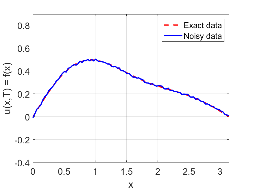
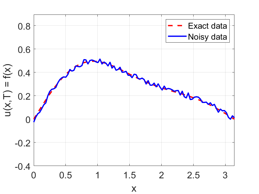
(a) Data, noise = 2%	(b) Data, noise = 5%
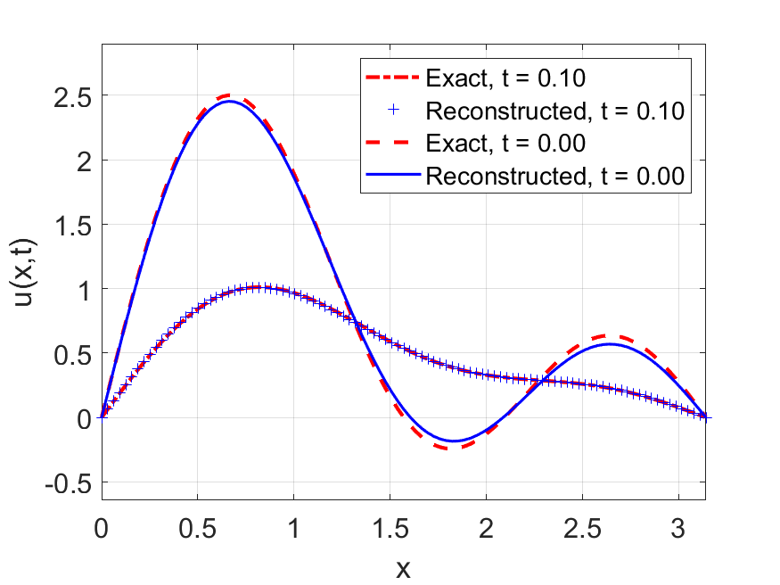
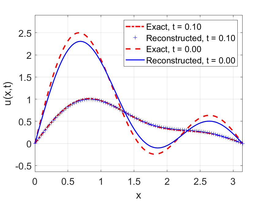
(c) a priori choice, noise = 2%	(d) a priori choice, noise = 5%
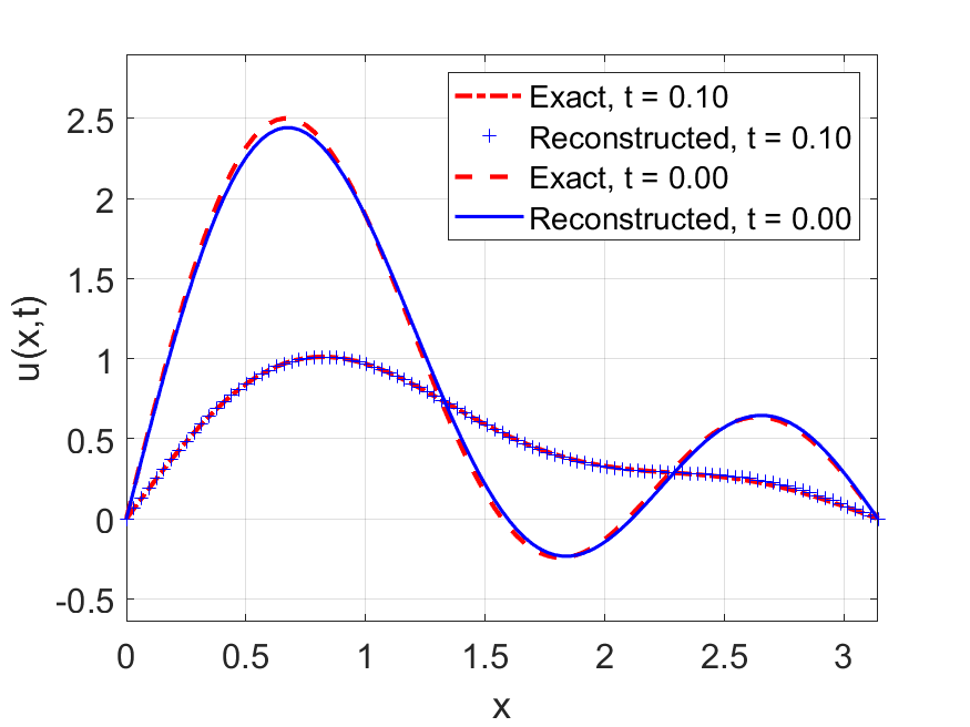
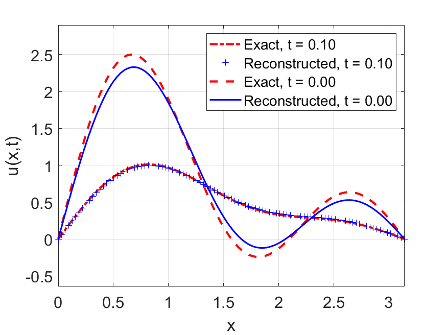
(e) a posteriori choice, noise = 2%	(f) a posteriori choice, noise = 5%

Figure 1: Reconstruction result for Example 1 for $\gamma=1/2$, $p=3$, $b=4$. Left column: noise = 2%; right column: noise = 5%.

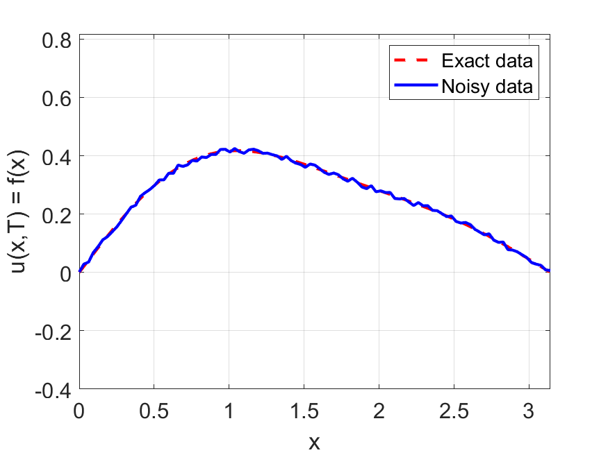
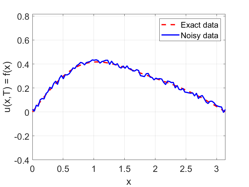
(a) Data, noise = 2%	(b) Data, noise = 5%
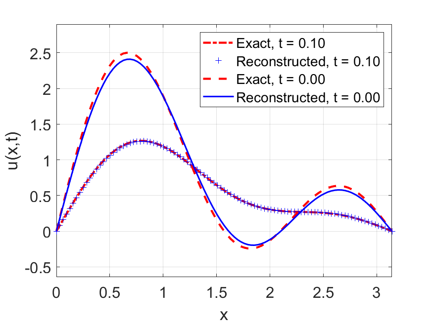
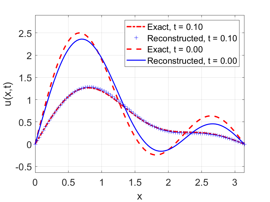
(c) a priori choice, noise = 2%	(d) a priori choice, noise = 5%
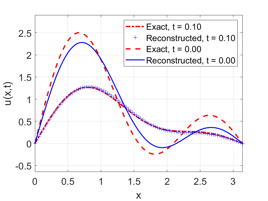
(e) a posteriori choice, noise = 2%	(f) a posteriori choice, noise = 5%

Figure 2: Reconstruction result for Example 1 for $\gamma=3/4$, $p=3$, $b=4$. Left column: noise = 2%; right column: noise = 5%.

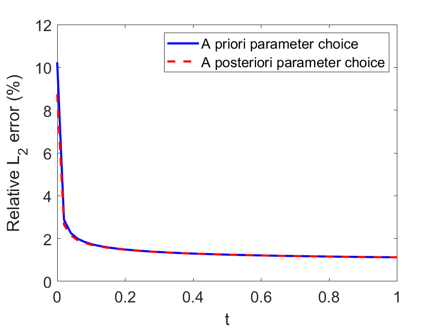
(a) $\gamma=1/2$	(b) $\gamma=3/4$.

Figure 3: Distribution of relative $L^{2}$-norm error over time for Example 1 with noise level = 5%. a) $\gamma=1/2$; b) $\gamma=3/4$. We can see that the error near $t=0$ is larger for larger $\gamma$. That means, the larger $\gamma$, the more ill-posed the backward problem.

Example 2: In this example we test the algorithm for another one dimensional problem which is described by the same equation as in (5.3) but the initial condition is given by

$$u(x,0)=u_{0}(x):=\begin{cases}x,&0\leq x<\pi/2,\\ \pi-x,&\pi/2\leq x\leq\pi.\end{cases}$$

It is easy to verify that

$$\left<u_{0},\phi_{n}\right>=\sqrt{\frac{2}{\pi}}\int_{0}^{\pi}u_{0}(x)\sin(nx)dx=\frac{2\sqrt{2}}{n^{2}\sqrt{\pi}}\sin(\frac{n\pi}{2}).$$

We approximated the solution of the forward problem (2.2) by (5.1) with $N_{p}=30$. In solving the backward equation, we again chose $N_{i}=5$ as in Example 1. We also chose $p=3$ and $b=4$.

The solution values of the backward problem at $t=0.1$ and $t=0$ are shown in Figure 4 for noise levels of $2\%$ and $5\%$. The figure shows that the reconstruction looks very accurate for both parameter choice rules at $t=0.1$ and reasonably good at $t=0$. These results are also comparable to the results obtained in Figure 6 of [6]. Note that due to the diffusion process, the nonsmooth initial condition is smoothed out rapidly in time, making the reconstruction of the nonsmooth behavior really challenging. We also observe that the a priori parameter choice gave more accurate reconstructions of the initial condition $u_{0}$, in particular, near the point $x=\pi/2$ at which the initial condition is not smooth. One possible reason for the this due to the approximation of operator $B_{\alpha}$ in calculating the regularization parameter $\alpha$ in the a posteriori choice, which may not result in the optimal value of $\alpha$.

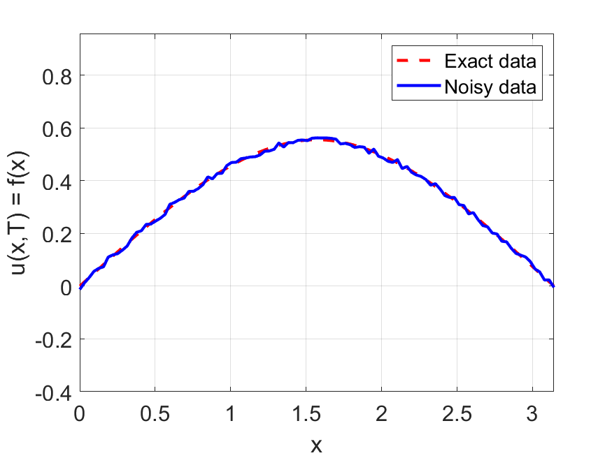
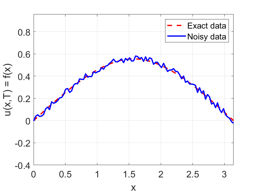
(a) Data, noise = 2%	(b) Data, noise = 5%
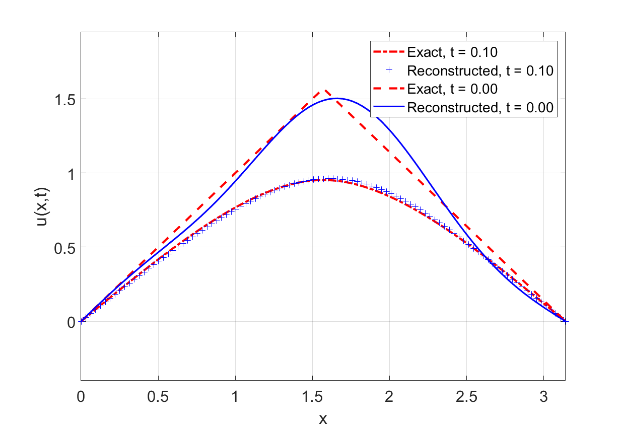
(c) a priori choice, noise = 2%	(d) a priori choice, noise = 5%
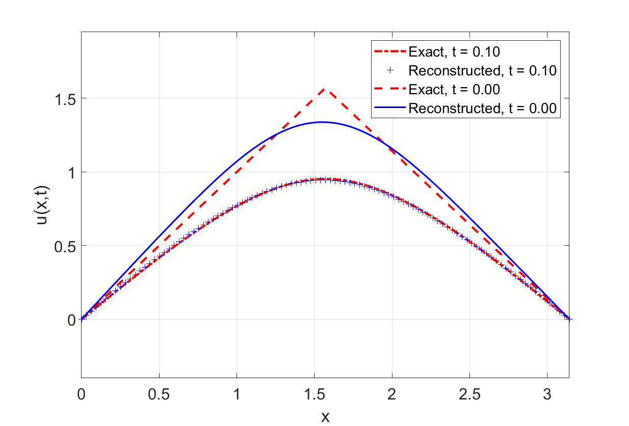
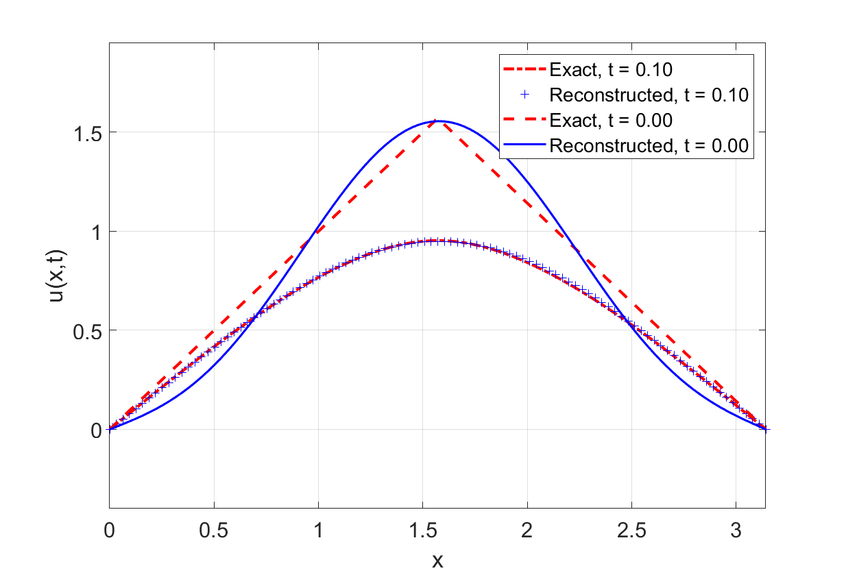
(e) a posteriori choice, noise = 2%	(f) a posteriori choice, noise = 5%

Figure 4: Reconstruction result for Example 2 for $\gamma=1/2$, $p=3$, $b=4$. Left column: noise = 2%; right column: noise = 5%.

Example 3: As the last numerical example, we tested the algorithm against the following two-dimensional problem

$$\frac{\partial^{\gamma}u(x,y,t)}{\partial t^{\gamma}} = \frac{\partial^{2}u(x,y,t)}{\partial x^{2}}+\frac{\partial^{2}u(x,y,t)}{\partial y^{2}},\quad x\in(0,\pi),\ y\in(0,\pi),\ t\in(0,T),$$

$$u(0,y,t) = u(\pi,y,t)=0,\quad y\in(0,\pi),\ t\in(0,T),$$ (5.4)

$$u(x,0,t) = u(x,\pi,t)=0,\quad x\in(0,\pi),\ t\in(0,T),$$

$$u(x,y,0) = u_{0}(x,y):=\sin(x)\sin(y)+\sin(2x)\sin(y),\quad x\in[0,\pi],\ y\in[0,\pi].$$

For this problem, the eigenvalues and eigenfunctions are given by

$$\lambda_{nm}=n^{2}+m^{2},\quad\phi_{nm}(x,y)=\frac{2\sin(nx)\sin(my)}{\pi},\quad n,m=1,2,\dots$$

The inner products $\left<u_{0},\phi_{nm}\right>$ are given by

$$\left<u_{0},\phi_{nm}\right>=\begin{cases}\pi/2,&n=1,2\text{ and }m=1,\\ 0,&\text{ otherwise}.\end{cases}$$

The implementation of the algorithm for this problem was similar to the one-dimensional case, except that we had to flatten the matrices of the eigenvalues and eigenfunctions to obtain one-dimensional arrays and then sorted them in the nondecreasing order. Note that in this example, there are repeated eigenvalues, but the corresponding eigenfunctions are not the same.

The reconstructions of the initial condition are shown in Figures 5-6 for two noise levels of $2\%$ and $10\%$ with $p=3$, $b=4$ and $\gamma=1/2$. In this example, we observed that $N_{i}=10$ is a good truncation number in solving the backward problem. The figures indicate that the initial condition was reconstructed accurately taking into account the noise levels in the measured data.

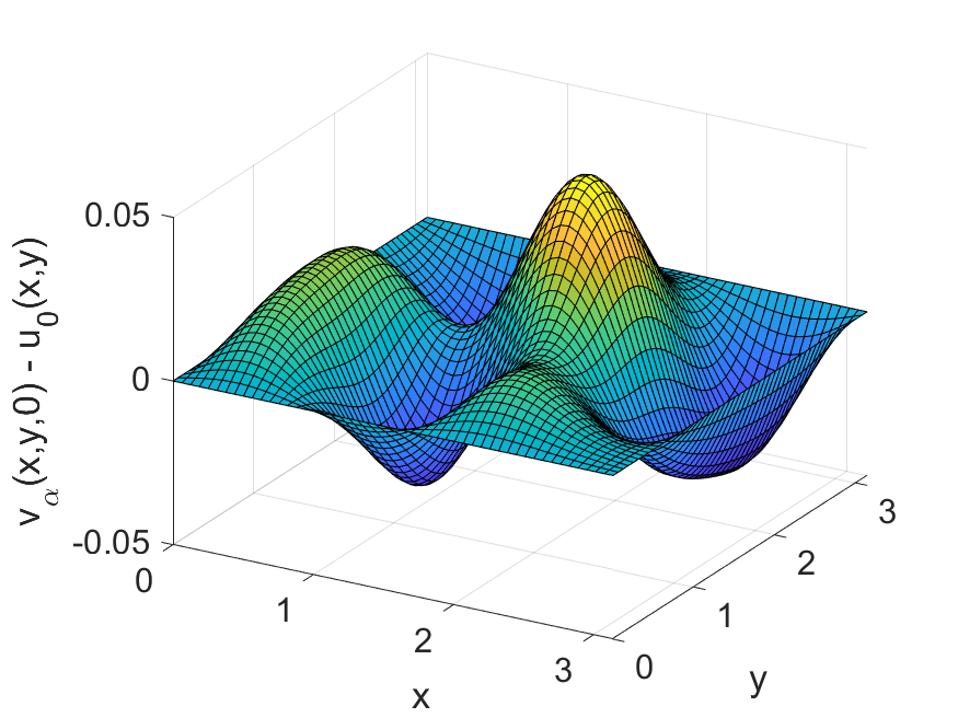
(a) Exact initial condition	(b) Error, a priori rule
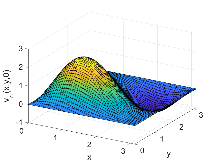
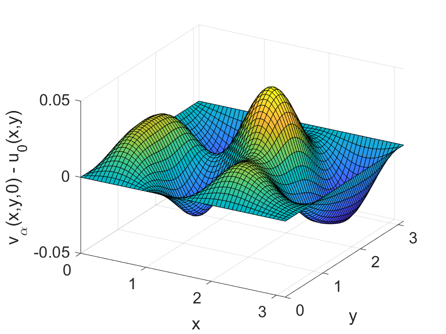
(c) Reconstruction, a priori rule	(d) Error, a posteriori rule
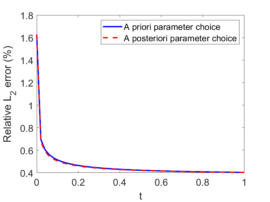
(e) Reconstruction, a posteriori rule	(f) $L^{2}$ error distribution in time

Figure 5: Reconstruction of the initial condition in Example 3 for $\gamma=1/2$, $p=3$, $b=4$ for noise level = 2% using the a priori parameter choice rule (c) and a posteriori parameter choice rule (e). The maximum error is about 2.5% and the $L^{2}$-norm error is about 1.6%. Both parameter choice rules produced almost the same results.

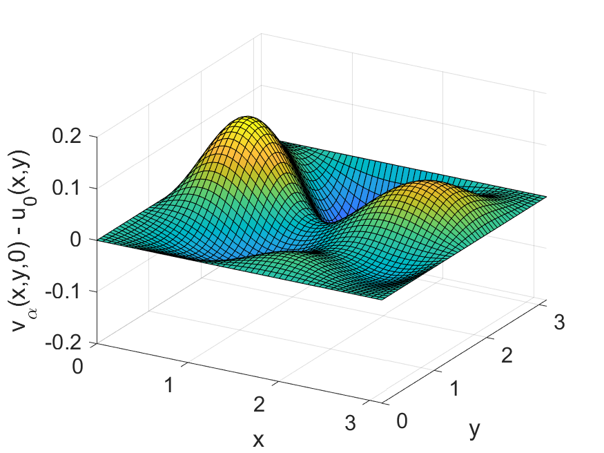
(a) Exact initial condition	(b) Error, a priori rule
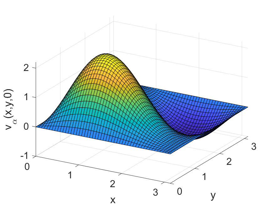
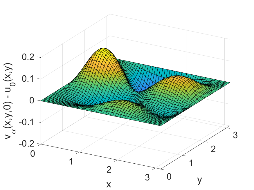
(c) Reconstruction, a priori rule	(d) Error, a posteriori rule
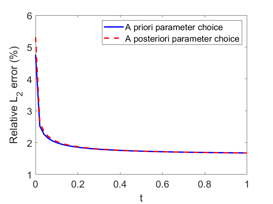
(e) Reconstruction, a posteriori rule	(f) $L^{2}$ error distribution in time

Figure 6: Reconstruction of the initial condition in Example 3 for $\gamma=1/2$, $p=3$, $b=4$ for noise level = 10% using the a priori parameter choice rule (c) and a posteriori parameter choice rule (e). The maximum error is about 10% and the $L^{2}$-norm error is about 5%. Both parameter choice rules produced almost the same results.

6 Conclusions

We regularized the backward time-fractional parabolic equations by Sobolev-type equations. We obtained optimal error estimates for the regularized solutions for both a priori and a posteriori regularization parameter choice rules. The theoretical error estimates were supported by numerical tests for one- and two-dimensional equations.

Acknowledgments. The work of N. V. Thang was partly supported by Vietnam National Foundation for Science and Technology Development (NAFOSTED) under grant number 101.01-2017.319.

References

- [1] M.F. Al-Jamal, A backward problem for the time-fractional diffusion equation. Math. Methods Appl. Sci. 40(2017), 2466–2474.
- [2] A. Chadha, D. Bahuguna, and D.N. Pandeym, Faedo-Galerkin approximate solutions for nonlocal fractional differential equation of Sobolev type. Fract. Differ. Calc. 8(2018), 205–222.
- [3] R. E. Ewing, The approximation of certain parabolic equations backward in time by Sobolev equations, SIAM J. Math.Anal., 6(1975),283–294.
- [4] M. A. Fury, Nonautonomous ill-posed evolution problems with strongly elliptic differential operators, Electron. J. Differential Equations, 92(2013), 1–25.
- [5] H. Gajewski and K. Zacharias, Zur Ruguliarisierung einer nichtkorrekter Probleme bei Evolutionsgleichungen, J. Math. Anal. Appl., 38(1972), 784–789.
- [6] D.N. Hào, J. Liu, N.V. Duc, and N.V. Thang, Stability results for backward time-fractional parabolic equations, Inverse Problems, 35(2019) 125006 (25pp).
- [7] Y. Huang and Z. Quan, Regularization for a class of illposed Cauchy problem, Proc. Amer. Math. Soc., 133(2005), 3005–3012.
- [8] B. Jin and W. Rundell, A tutorial on inverse problems for anomalous diffusion processes, Inverse Problems, 31(2015) 035003 (40pp).
- [9] N. T. Long and A. P. N. Dinh, Approximation of a parabolic non-linear evolution equation backward in time, Inverse Problems, 10 (1994), 905–914.
- [10] N. T. Long and A. P. N. Dinh, Note on a regularization of a parabolic nonlinear evolution equation backwards in time, Inverse Problems, 4(1996), 455–462.
- [11] A.A. Kilbas, H.M. Srivastava, J.J. Trujillo, Theory and Applications of Fractional Differential Equations, Elsevier, 2006.
- [12] J.J. Liu and M. Yamamoto, A backward problem for the time-fractional diffusion equation, Appl. Anal. 89(2010), 1769–1788.
- [13] V. Padrón, Sobolev regularization of some nonlinear illposed problems, PhD thesis. University of Minnensota, Minneapolis, 1990.
- [14] V. Padrón, Sobolev regularization of a nonlinear ill-posed parabolic problem as a model for aggregating populations, Commun. Partial Differential Equations, 23(1998),457–486.
- [15] I. Podlubny, Fractional Differential Equatins: An Introduction to Fractional Derivatives, Fractional Differential Equations, to Methods of Their Solution and Some of Their Applications, Academic Press, 1999.
- [16] M. Renardy and R. C. Rogers, An Introduction to Partial Differential Equations, 2nd Edition, Springer-Verlag, New York Inc. 2004.
- [17] K. Sakamoto and M. Yamamoto, Initial value/boundary value problems for fractional diffusion-wave equations and applications to some inverse problems, J. Math. Anal. Appl. 382(2011), 426–447.
- [18] R. E. Showalter, The final value problem for evolution equations, J. Math. Anal. Appl. 47 (1974) 563–572.
- [19] L. Wang and J. Liu, Data regularization for a backward time-fractional diffusion problem, Comput. Math. Appl. 64(2012),3613–3626.
- [20] L. Wang and J. Liu, Total variation regularization for a backward time-fractional diffusion problem, Inverse Problems 29(2013), 115013, 22pp.
- [21] J.G. Wang, T. Wei , Y.B. Zhou, Tikhonov regularization method for a backward problem for the time-fractional diffusion equation, Appl. Math. Model. 37(2013), 8518 -8532.
- [22] J.G. Wang, T. Wei, Y.B. Zhou, Optimal error bound and simplified Tikhonov regularization method for a backward problem for the time-fractional diffusion equation, J. Comput. Appl. Math. 279(2015), 277–292.
- [23] J. G. Wang, Y. B. Zhou, T. Wei, A posteriori regularization parameter choice rule for the quasi-boundary value method for the backward time-fraction diffusion problem, Appl. Math. Lett. 26(2013), 741–747.
- [24] T. Wei and J.G. Wang, A modified quasi-boundary value method for the backward time-fractional diffusion problem, ESAIM Math. Model. Numer. Anal. 48(2014), 603–621.
- [25] M. Yang and J. Liu, Solving a final value fractional diffusion problem by boundary condition regularization, Appl. Numer. Math. 66(2013), 45–58.
- [26] M. Yang and J. Liu, Fourier regularization for a final value time-fractional diffusion problem, Appl. Anal. 94(2015), 1508–1526.