Why integral equations should be used instead of differential equations to describe the dynamics of epidemics

Abstract

It is of vital importance to understand and track the dynamics of rapidly unfolding epidemics. The health and economic consequences of the current COVID-19 pandemic provide a poignant case. Here we point out that since they are based on differential equations, the most widely used models of epidemic spread are plagued by an approximation that is not justified in the case of the current COVID-19 pandemic. Taking the example of data from New York City, we show that currently used models significantly underestimate the initial basic reproduction number ($R_{0}$). The correct description, based on integral equations, can be implemented in most of the reported models and it much more accurately accounts for the dynamics of the epidemic after sharp changes in $R_{0}$ due to restrictive public congregation measures. It also provides a novel way to determine the incubation period, and most importantly, as we demonstrate for several countries, this method allows an accurate monitoring of $R_{0}$ and thus a fine-tuning of any restrictive measures. Integral equation based models do not only provide the conceptually correct description, they also have more predictive power than differential equation based models, therefore we do not see any reason for using the latter.

Introduction

A commonly used approach to describe the dynamics of epidemics is based on SEIR-type (Susceptible-Exposed-Infectious-Recovered) differential equations [1, 2, 3, 4, 5]. Recently these methods have been applied to the COVID-19 pandemic to determine the basic reproduction number [6, 7, 8, 9, 10, 11], the incubation period [12, 13, 14] and to describe the dynamics of the pandemic [15, 16, 17, 18, 19, 20, 21, 22]. In this framework there is no natural and transparent way to account for the delay between the introduction of public health measures and the corresponding change in the newly reported cases. This delay occurs due to the incubation period of the disease. Even after refinements to try to account for some aspects of this delay [23, 15, 16, 17], these models are still plagued by uncontrolled approximations. We suggest that models based on differential equations should be replaced with ones based on an integral equation, which explains the time delay without any additional step or input. The approach we present is not completely new, it was already implicit in the original Kermack-McKendric theory proposed in 1927 [24]. Even though several variants of that model with various degrees of precision circulate in the current literature [25, 26, 27, 28], their superiority over the differential equation based method has not been widely recognised.

We emphasise that in the form presented below, the integral equation based approach is neither technically nor conceptually more complicated than the one based on differential equations. More importantly, it gives a much more realistic representation of the epidemic dynamics. We demonstrate this by comparing how the two types of approach describe the New York City data [29], taken from the currently ongoing COVID-19 pandemic. Firstly, we show that even in the initial simple exponential phase of the epidemic, the correct, integral equation based model can give a significantly larger estimate for $R_{0}$, the basic reproduction number. Secondly, we show that the oscillations in the graph of the number of newly infected people after restrictive public interaction measures are introduced, is well described by the integral equation model. This is a generic feature of COVID-19 data, seen in several countries, and there is no simple way the differential equation based models could explain it. Thirdly, using data of several countries, we illustrate how the change of $R_{0}$ in time can be monitored using the integral equation formalism.

Our comparison here is based on a simple SEIR-type differential equation model and its integral equation counterpart containing the same variables, but a different time evolution. It can be seen from our general discussion that the differences we find are generic features of the two types of models and carry over to more sophisticated versions thereof. We urge everyone to test how different their results are between the two approaches in the case of the particular models they use.

Integral equation description for discrete and continuous time evolution

Figure 1: The number of new infections per day, shown up to the eleventh (top) and the twelfth day (bottom) of the epidemic. The blue area represents those that are infected, but not yet infectious, i.e. people who were exposed between today and $t_{e}=4$ days ago. The red area represents those that are infectious, i.e. people who were exposed more than $t_{e}$ days ago, but not more than $t_{e}+t_{i}=7$ days ago. In the SEIR model the number of people who cease to be infectious from day 11 to day 12 is equal to the daily average of the red area in the top panel. In reality, however, only people in the leftmost red histogram, here a much smaller number, cease to be infectious. Similarly, in the SEIR model the number of people who become infectious is the daily average of the blue area, when in reality it is only people in the leftmost bar of the blue area who become infectious from day 11 to day 12. Clearly the only case when the SEIR model correctly represents the situation is when the number of newly infected people per day is constant in time.

The mathematical modelling of how infectious diseases spread is almost exclusively based on compartmental models. In this framework the population is divided into different categories and a dynamical model is set up to describe how the number of individuals in each category evolves with time. A simple model of this type is the so called SEIR model, in which the compartments are susceptible (not yet infected), exposed and infected (but not yet capable of infecting others), infectious, and recovered/removed (not capable of infecting others any more). In its simplest form the model is characterised by three parameters, $\alpha,\beta,\gamma$ that determine the transition rates among different compartments through the following set of differential equations:

$$\frac{dS}{dt}=-\beta\frac{I}{N}S,\;\;\;\;\;\frac{dE}{dt}=\beta\frac{I}{N}S-\alpha E,\;\;\;\;\;\frac{dI}{dt}=\alpha E-\gamma I,\;\;\;\;\;\frac{dR}{dt}=\gamma I,$$ (1)

where $S(t),E(t),I(t)$ and $R(t)$ are the number of susceptible, exposed, infectious and recovered individuals, all functions of the time, and $N=S+E+I+R$ is the total population.

In the initial phase of a rapidly developing epidemic, the situation we are concerned with here, $S/N\approx 1$, which we will assume. With this approximation the two functions describing the dynamics are $E(t)$ and $I(t)$. At this point it is instructive to introduce $t_{e}$ and $t_{i}$, the average days an individual spends in the categories $E$ and $I$ respectively. It is convenient to write the equations in terms of these parameters and the basic reproduction number, $R_{0}$, using the simple relations $\alpha=1/t_{e}$, $\beta=R_{0}/t_{i}$ and $\gamma=1/t_{i}$.

With these new parameters the simplified form of the differential equations valid for the initial stage when $S/N\approx 1$ is

$$\frac{d}{dt}\begin{pmatrix}E\\ I\end{pmatrix}=\begin{pmatrix}-1/t_{e}&R_{0}/t_{i}\\ 1/t_{e}&-1/t_{i}\end{pmatrix}\begin{pmatrix}E\\ I\end{pmatrix}.$$ (2)

The SEIR equations are based on the assumption that the transition rates between compartments are proportional to the number of people in those compartments. Furthermore, all people in a compartment are treated equally, irrespective of how much time they already spent there. These assumptions are only correct when $R_{0}$ is close to 1 and changes slowly. In the following we derive the integral equation description of epidemics.

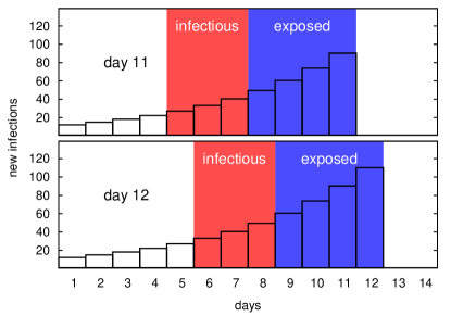
Let us denote the number of newly infected individuals on day $t$ by $\rho(t)$. The function $\rho(t)$ contains the entire history of infections. This can be depicted in a histogram with time flowing from left to right along the horizontal axis (Fig. 1). Based on this information we would like to determine $\rho(t+1)$, the number of individuals becoming infected on the following day. As in the SEIR model above let us here also assume that anyone exposed to the infection will become infected, but will not be infectious for $t_{e}$ days. Such a person will become infectious $t_{e}$ days after exposure and will remain in this category for an additional $t_{i}$ days, after which he is isolated and ceases to be capable of infecting others. In the simplest version of the model $t_{e}$ and $t_{i}$ can represent averages, but later on we will indicate how to generalise the model by using continuous distributions. In Fig. 1 the blue area represents those in category $E$, with $t_{e}=4$, and the red area those in $I$, with $t_{i}=3$. Now, exactly as in the SEIR model above, the number of newly infected on the following day, day 12 in the figure, will be

$$\rho(t+1)=\beta\sum_{\tau=t-t_{i}-t_{e}+1}^{t-t_{e}}\rho(\tau),\hskip 25.83325pt\beta=\frac{R_{0}}{t_{i}}$$ (3)

where the sum is the total number of infectious individuals at time $t$, i.e. the red area in the top panel of Fig. 1. At this point we can depict the situation at time $t+1$ simply by shifting both the blue and the red region, showing the people in category $E$ and $I$, one day forward to the right (bottom panel of Fig. 1). From this point on the same procedure can be further iterated day by day: on each day we calculate the number of newly infected for the following day and shift the windows delineating the exposed and the infectious by one day forward.

At this point the objection could be raised that we have been comparing the continuous SEIR model with a discretised model. However, the framework presented in the histograms can be easily generalised from days to arbitrarily fine time steps. In the limit of infinitely fine time steps $dt$, we can choose the height of the histogram bars $\rho(t)$ such that $\rho(t)dt$ be the number of people becoming infected in the time interval $[t,t+dt]$. In this case the sum in the right hand side of Eq. (3) becomes an integral and the equation can be rewritten as

$$\rho(t)=\beta\int_{t-t_{i}-t_{e}}^{t-t_{e}}\rho(\tau)\,d\tau,\hskip 25.83325pt\beta=\frac{R_{0}}{t_{i}}.$$ (4)

We emphasise that only this continuous version of the model describes the real situation properly.

Figure 2: $R_{0}$ as a function of $t_{i}$, the infectious part of the incubation period. The total incubation period is taken to be $t_{e}+t_{i}$=6.4 days [13] and the exponential growth parameter is $1/\lambda=1.78$ days which describe the growing phase of the New York City data [29] well. The orange colour curve with the maximum shows the prediction (5) based on the SEIR model of eq. (2). The blue and red lines correspond to the analytic solution (5) of the integral equation (4) and its discretised version (3) with an hourly time step, respectively. Their agreement indicate that such a discretisation is sufficient. A daily discretisation would give 34% higher $R_{0}$ values.

Determination of $R_{0}$, the example of New York City

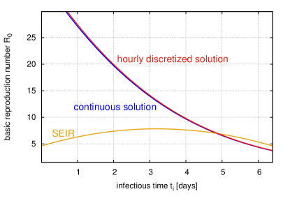
We illustrate the shortcomings of the SEIR model in two examples. First let us consider the case of constant $R_{0}>1$ which leads to the exponentially growing solution with exponent $\lambda$, i.e. all relevant quantities ($E(t),I(t)$ of SEIR and $\rho(t)$ of the integral equation) are proportional to $\exp(\lambda t)$. A simple substitution gives:

$$R_{0}^{(\mbox{\scriptsize SEIR})}=1+\lambda(t_{e}+t_{i})+\lambda^{2}\cdot t_{e}t_{i},\quad R_{0}^{(\mbox{\scriptsize integral})}=\frac{t_{i}\lambda}{e^{-\lambda t_{e}}-e^{-\lambda(t_{e}+t_{i})}},\quad R_{0}^{(\mbox{\scriptsize discretised})}=\frac{e^{\lambda\Delta t}-1}{\lambda\Delta t}R_{0}^{(\mbox{\scriptsize integral})},$$ (5)

where $R_{0}^{(\mbox{\scriptsize discretised})}$ is the solution of the discretised equation (3) with time step $\Delta t$. Figure 2 shows these three $R_{0}$ (SEIR, integral equation, discretised integral equation) obtained using realistic parameters that describe the initial phase of the pandemic in New York City. There is a striking difference between the SEIR and integral equation predictions. While the SEIR result is largely insensitive to the split of the total incubation period into $t_{e}$ and $t_{i}$, this is not the case for the solution of the integral equation. The true value of $R_{0}$ can be 3-4 times larger than the one predicted by the SEIR model. For $t_{i}\approx 2$ days which, as we will later see, provides a reasonable description of the daily reported cases, $R_{0}$ can be as high as 20. $R_{0}$ is, of course region dependent. Less populated areas can have much smaller $R_{0}$ values.

One might think that this difference is only due to the relatively large incubation period (as compared to the characteristic growth time of the pandemic) and the SEIR model gives reliable estimates for small incubation periods. Surprisingly this is not the case. A trivial expansion of $R_{0}^{(\mbox{\scriptsize integral})}$ in $\lambda t_{e}$ and $\lambda t_{i}$ yields $R_{0}^{(\mbox{\scriptsize integral})}\approx 1+\lambda(t_{e}+t_{i}/2)+\lambda^{2}(t_{e}^{2}/2+t_{e}t_{i}/2+t_{i}^{2}/12)+{\cal O}(\lambda^{3})$ which is clearly different from the SEIR result.

The effect of decreasing $R_{0}$, delay and oscillation

Figure 3: Left: time evolution of new reported cases after a lockdown on day 73 in the case of the SEIR and integral equation models. For the initial phase of the pandemic $1/\lambda=1.78$ days, $t_{e}=4.4$ days and $t_{i}$=2 days was used. This corresponds to $R_{0}^{\mbox{\scriptsize SEIR}}=7.37$ and $R_{0}^{\mbox{\scriptsize integral}}=19.7$. The value of $R_{0}$ was instantaneously decreased to $0.95$ in both cases on day 73. The difference between the two models is quite dramatic. The SEIR solution reacts immediately and turns smoothly to a decreasing exponential function. The solution of the integral equation is qualitatively different. There is a delay of $t_{e}+t_{i}$ after which the effect of the lockdown becomes visible, then an oscillation follows. The characteristic scales of this oscillation are indicated in the figure. Right: time evolution of the new reported cases after a gradual lockdown from day 71 to day 74 confronted with the data of New York City. The initial parameters are the same as for the left panel. $R_{0}$ is now decreased to $0.95$ linearly in time during this four day period in both models (for a detailed analysis how $R_{0}$ changed and dropped to a smaller value in New York City see later). The main features of the curves are similar to the left panel but the amplitude of the oscillation is reduced, making it similar to the real data. Note that we did not fit our model to the data. This plot is an illustration that the main features (delay and oscillation) of the data are well captured by the integral equation and neither of these is reproduced by SEIR.

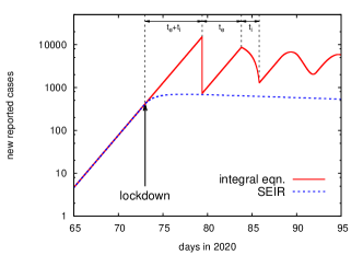
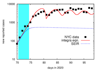
The parameter $R_{0}$ in both the SEIR- and the integral equations is in general time dependent. The most important goal of the first restrictive measures was to decrease the value of $R_{0}$ as fast as possible and bring it below the critical value of $1$. In the following we study how the different models react to a sudden drop of $R_{0}$ and compare them qualitatively to the daily reported new cases in New York City [29]. To simplify our discussion we will assume that all cases are reported exactly after the incubation period, i.e. $t_{e}+t_{i}$ days after first exposure. In the case of the SEIR model the rate of people leaving the incubation period is $dR/dt=\gamma I$ while in the case of the integral equation it is $\rho(t-t_{e}-t_{i})$. These two functions will be referred to as ”new reported cases” in the following. If we assume that the majority of cases are reported when symptoms emerge, it follows that any change in the parameters will only show up $t_{e}+t_{i}$ days later in the data. Any reasonable model should be able to naturally account for this delay. Quantities in differential equations react immediately to any change of the parameters, thus no differential equation based model (such as SEIR or its simple extensions) is expected to explain such a delay. The integral equation (4), on the other hand, naturally provides a delay.

The simplest possibility is to assume that $R_{0}$ decreases instantaneously after a successful lockdown. The left panel of Figure 3 shows how the number of reported new cases evolves after a lockdown happens on March 13 (day 73 of 2020) which reduces $R_{0}$ to 0.95. A more realistic situation is shown in the right panel of Figure 3. Here the value of $R_{0}$ was gradually decreased from March 11 to March 14. In both cases the expected delay, which is clearly visible in the data, is only explained by the integral equation. The reported data of many countries show an interesting oscillation after the effect of a lockdown starts to show up. This feature is also naturally described by the integral equation.

One remark is in order. The incubation period of 6.4 days is accidentally very close to the weakly cycle of 7 days. Thus, the oscillation might in principle be just a weekend effect. Looking at the weekend during the strongly exponential growth with enough statistics (March 14, Saturday to March 16, Monday) one observes less cases during Saturday and Sunday and an accordingly higher number of cases on Monday than the average exponential growth would predict. Correcting the data for this effect later would weaken but not eliminate the observed oscillation, it seems to be a real effect. This is also supported by the fact that different countries have minima and maxima of their oscillation on different days (e.g. in Italy the minima are on Mondays and Tuesdays, in the Netherlands they are on Tuesdays and Wednesdays).

It is in principle possible to determine the incubation time $t_{e}$ and $t_{i}$ from this oscillatory pattern. Taking the distance of subsequent minima we determined $t_{e}+t_{i}$. Using data of New York City, Italy, Spain, Germany, and the Netherlands [29, 30] the period of the oscillations seems quite robust and is around $t_{e}+t_{i}=7.4$ days on average with a spread of 0.2 days.

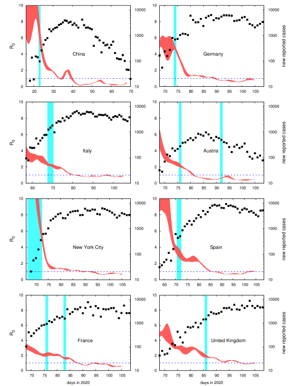
Once $t_{e}$ and $t_{i}$ are known, one can solve eqn (4) for $\beta(t)$ or equivalently $R_{0}(t)$ by taking $\rho(t)$ and the (numerical) integral from the actual data:

$$R_{0}(t)=\frac{t_{i}\rho(t)}{\int_{t-t_{e}-t_{i}}^{t-t_{e}}\rho(\tau)d\tau}.$$ (6)

In this way one can continuously monitor the effect of restrictive or easing measures. We used this procedure to analyse data from seven countries as well as New York City. In each country the raw data for the daily number of new infections shows large daily fluctuations, most likely due to some anomalies in reporting new cases. In order to remove these fluctuations we performed the following smearing procedure. If the original data is given by $\bar{\rho}(t)$ then we replace this by $w\bar{\rho}(t-1)+(1-2w)\bar{\rho}(t)+w\bar{\rho}(t+1)$ and repeat this procedure three times. We checked that the function $R_{0}(t)$ depends only mildly on the choice of $w$. The results, for which we used $w=0.25$ are shown in Figure 4.

For all regions we can observe a large drop in $R_{0}$. However, while in China $R_{0}$ went significantly below 1, effectively stopping the epidemic, in European countries and New York City it is just below or around 1 even today. It seems inevitable that in these regions any significant easing of the restrictions will induce a second wave of the epidemic. An accurate monitoring of $R_{0}$ is extremely important in this situation. As demonstrated above, the integral equation formulation is the right approach here.

Figure 4: Determination of the basic reproduction number $R_{0}$ as a function of time for China, Germany, Italy, Austria, New York City, Spain, France and the United Kingdom. We used the integral equation (4) to compute $R_{0}$ from the available data [30, 31, 29]. The red bands show the results. We varied $t_{i}$ between 1 and 2 days and $t_{e}+t_{i}$ between 6.5 and 7.5 days. The uncertainty associated with this variation is shown by the widths of the bands. As an illustration the cyan areas show the approximate time periods when well defined restrictive measures were introduced within a short time interval (lockdown of Hubei province in China (January 23), lockdown of Lombardy (March 8) and the whole of Italy (March 10), closing schools in Germany (March 14), nationwide curfew (March 16) and compulsory wearing of masks (April 1) in Austria, state of emergency (March 7) and closing of Broadway theatres (March 12) in New York City, closing schools in Spain (March 11-12), closing schools (March 16) and restriction of movement (March 23) in France, and issuing statutory instrument 350 in the UK (March 26)). For completeness the original data are also shown (right vertical axes). Clearly as health authorities are getting better and better data the accuracy on $R_{0}$ determination will improve.

Conclusions and Outlook

In the previous sections we compared the SEIR model and the integral equation when both $t_{e}$ and $t_{i}$ are fixed. In reality the incubation period is described by a probability function $P(\tau)$ which gives the probability that a person is infectious a time $\tau$ after exposure. The integral equation (4) can easily be generalised to include $P$:

$$\rho(t)=\beta\int_{0}^{\infty}\rho(t-\tau)P(\tau)d\tau,\qquad\qquad R_{0}=\beta\int_{0}^{\infty}P(\tau)d\tau.$$ (7)

In general, the transmission rate $\beta$ also changes in time since new restrictive measures can be implemented. This can also be incorporated into the equation, however, in that case $R_{0}$ might not have a transparent interpretation. This equation has been around in the literature for a long time (see e.g. [25, 26, 27]) but unfortunately it has not yet been widely adopted. Any evolution computed using this equation is expected to have qualitatively similar features (delay and oscillation) as in the simple approximation presented above. The SEIR model is not a good approximation of this integral equation even if the $P(\tau)$ probability is built into its parameters.

For later stages of a pandemic when $S/N<1$ the integral equation can be generalised to include $S$ as well. Furthermore, one can divide the population into sub-compartments e.g. by age groups or location. Each sub-compartment with a population of $N_{i}$ can be described by its own $\rho_{i}(t)$ infection history and $P_{i}(\tau)$ probability function and the cross infection rates between compartments $j$ and $i$ by $\beta_{i\leftarrow j}$. The generalised coupled integral equations in this case read:

$$\rho_{i}(t)=\frac{S_{i}(t)}{N_{i}}\sum_{j}\beta_{i\leftarrow j}\int_{0}^{\infty}\rho_{j}(t-\tau)P_{j}(\tau)d\tau,\qquad S_{i}(t)=N_{i}-\int_{-\infty}^{t}\rho_{i}(\tau)d\tau.$$ (8)

As an example, we ran some simulations of the full course of the epidemic until $S$ saturated close to zero. We found that depending on the parameters the integral equation and the SEIR equations can predict a significantly different maximal number of cases at the peak of the epidemic. Any further extension which can be included in the SEIR equations (e.g. birth and death rate, day/night differences, inhomogeneities, meta-population systems, etc.) can also be naturally included in the integral equation formalism.

We demonstrated that the approximation leading to differential equation based models of epidemic spread is not sufficient in the case of the COVID-19 pandemic. In particular, differential equations provide a good description only if $R_{0}$ is close to 1 and if it changes only slowly compared to the incubation period of the disease. Note that even if $R_{0}$ is larger than 1, the initial exponential phase of the epidemic can be well described by differential equations, but they can significantly underestimate the value of $R_{0}$, the larger the $R_{0}$, the more so. If, however, as a result of restrictive measures, $R_{0}$ suddenly drops, differential equations fail to describe the ensuing oscillatory behaviour of the number of new cases and as a result, they are not suitable for a precise monitoring of $R_{0}$. In contrast, integral equations are naturally suited to this task, even if sharp changes occur in $R_{0}$. We also presented a simple way to implement the integral equation formalism in numerical simulations, which do not become more complicated than the numerical solution of the SEIR equations. In summary, the integral equation approach has more predictive power than the most widely used differential equation based models and also eliminates a serious uncontrolled approximation of the latter. In the light of the present results we urge practitioners of the field to rethink and possibly consider implementing the integral equation based technique.

References

- [1] R. Anderson, R. May, Infectious Diseases of Humans: Dynamics and Control, Dynamics and Control (OUP Oxford, 1992).
- [2] M. Lipsitch, et al., Transmission dynamics and control of severe acute respiratory syndrome, Science 300, 1966 (2003). https://doi.org/10.1126/science.1086616.
- [3] J. T. Wu, B. J. Cowling, The use of mathematical models to inform influenza pandemic preparedness and response, Experimental Biology and Medicine 236, 955 (2011). https://dx.doi.org/10.1258/ebm.2010.010271.
- [4] C. Fraser, et al., Pandemic potential of a strain of influenza a (h1n1): early findings, science 324, 1557 (2009). https://doi.org/10.1126/science.1176062.
- [5] P. Klepac, et al., Stage-structured transmission of phocine distemper virus in the dutch 2002 outbreak, Proceedings of the Royal Society B: Biological Sciences 276, 2469 (2009). https://doi.org/10.1098/rspb.2009.0175.
- [6] J. T. Wu, K. Leung, G. M. Leung, Nowcasting and forecasting the potential domestic and international spread of the 2019-ncov outbreak originating in wuhan, china: a modelling study, The Lancet 395, 689 (2020). https://doi.org/10.1016/S0140-6736(20)30260-9.
- [7] B. Tang, et al., Estimation of the transmission risk of the 2019-ncov and its implication for public health interventions, Journal of Clinical Medicine 9, 462 (2020). https://doi.org/10.3390/jcm9020462.
- [8] B. Tang, et al., An updated estimation of the risk of transmission of the novel coronavirus (2019-ncov), Infectious disease modelling 5, 248 (2020). https://doi.org/10.1016/j.idm.2020.02.001.
- [9] Q. Li, et al., Early transmission dynamics in wuhan, china, of novel coronavirus–infected pneumonia, New England Journal of Medicine (2020). https://doi.org/10.1056/NEJMoa2001316.
- [10] H. Wang, et al., Phase-adjusted estimation of the number of coronavirus disease 2019 cases in wuhan, china, Cell Discovery 6, 1 (2020). https://doi.org/10.1038/s41421-020-0148-0.
- [11] A. J. Kucharski, et al., Early dynamics of transmission and control of covid-19: a mathematical modelling study, The lancet infectious diseases (2020). https://doi.org/10.1016/S1473-3099(20)30144-4.
- [12] S. A. Lauer, et al., The incubation period of coronavirus disease 2019 (covid-19) from publicly reported confirmed cases: estimation and application, Annals of internal medicine (2020). https://doi.org/10.7326/M20-0504.
- [13] J. A. Backer, D. Klinkenberg, J. Wallinga, Incubation period of 2019 novel coronavirus (2019-ncov) infections among travellers from wuhan, china, 20–28 january 2020, Eurosurveillance 25 (2020). https://doi.org/10.2807/1560-7917.ES.2020.25.5.2000062.
- [14] N. M. Linton, et al., Incubation period and other epidemiological characteristics of 2019 novel coronavirus infections with right truncation: a statistical analysis of publicly available case data, Journal of clinical medicine 9, 538 (2020). https://doi.org/10.3390/jcm9020538.
- [15] M. Chinazzi, et al., The effect of travel restrictions on the spread of the 2019 novel coronavirus (covid-19) outbreak, Science (2020). https://doi.org/10.1126/science.aba9757.
- [16] M. U. Kraemer, et al., The effect of human mobility and control measures on the covid-19 epidemic in china, Science (2020). https://doi.org/DOI:10.1126/science.abb4218.
- [17] K. Prem, et al., The effect of control strategies to reduce social mixing on outcomes of the covid-19 epidemic in wuhan, china: a modelling study, The Lancet Public Health (2020). https://doi.org/10.1016/S2468-2667(20)30073-6.
- [18] R. Li, et al., Substantial undocumented infection facilitates the rapid dissemination of novel coronavirus (sars-cov2), Science (2020). https://doi.org/10.1126/science.abb3221.
- [19] Z. Yang, et al., Modified seir and ai prediction of the epidemics trend of covid-19 in china under public health interventions, Journal of Thoracic Disease 12, 165 (2020). https://doi.org/10.21037/jtd.2020.02.64.
- [20] P. Boldog, et al., Risk assessment of novel coronavirus covid-19 outbreaks outside china, Journal of clinical medicine 9, 571 (2020). https://doi.org/10.3390/jcm9020571.
- [21] R. M. Anderson, H. Heesterbeek, D. Klinkenberg, T. D. Hollingsworth, How will country-based mitigation measures influence the course of the covid-19 epidemic?, The Lancet 395, 931 (2020). https://doi.org/10.1016/S0140-6736(20)30567-5.
- [22] S. M. Kissler, C. Tedijanto, E. Goldstein, Y. H. Grad, M. Lipsitch, Projecting the transmission dynamics of sars-cov-2 through the postpandemic period, Science (2020). https://doi.org/10.1126/science.abb5793.
- [23] L. Wang, J. Wu, Characterizing the dynamics underlying global spread of epidemics, Nature Communications 9, 218 (2018). https://doi.org/10.1038/s41467-017-02344-z.
- [24] W. O. Kermack, A. G. McKendrick, A contribution to the mathematical theory of epidemics, Proceedings of the royal society of london. Series A, Containing papers of a mathematical and physical character 115, 700 (1927). https://doi.org/10.1098/rspa.1927.0118.
- [25] H. W. Hethcote, D. W. Tudor, Integral equation models for endemic infectious diseases, Journal of mathematical biology 9, 37 (1980). https://doi.org/10.1007/BF00276034.
- [26] H. J. Wearing, P. Rohani, M. J. Keeling, Appropriate models for the management of infectious diseases, PLoS medicine 2, 621 (2005). https://doi.org/10.1371/journal.pmed.0020174.
- [27] J. Wallinga, M. Lipsitch, How generation intervals shape the relationship between growth rates and reproductive numbers, Proceedings of the Royal Society B: Biological Sciences 274, 599 (2007). https://dx.doi.org/10.1098%2Frspb.2006.3754.
- [28] S. Flaxman, et al., Report 13: Estimating the number of infections and the impact of non-pharmaceutical interventions on covid-19 in 11 european countries (2020). https://doi.org/10.25561/77731.
- [29] New York City webpage: https://www1.nyc.gov/site/doh/covid/covid-19-data.page.
- [30] European Centre for Disease Prevention and Control webpage: https://www.ecdc.europa.eu/en/publications-data/download-todays-data-geographic-distribution-covid-19-cases-worldwide.
- [31] For the daily reported cases in Austria we used: https://info.gesundheitsministerium.at.