Interpreting neural network models of residual scalar flux

Abstract

We show that in addition to providing effective and competitive closures, when analysed in terms of dynamics and physically-relevant diagnostics, artificial neural networks (ANNs) can be both interpretable and provide useful insights in the on-going task of developing and improving turbulence closures. In the context of large-eddy simulations (LES) of a passive scalar in homogeneous isotropic turbulence, exact subfilter fluxes obtained by filtering direct numerical simulations (DNS) are used both to train deep ANN models as a function of filtered variables, and to optimise the coefficients of a turbulent Prandtl number LES closure. A-priori analysis of the subfilter scalar variance transfer rate demonstrates that learnt ANN models out-perform optimised turbulent Prandtl number closures and Clark-type gradient models. Next, a-posteriori solutions are obtained with each model over several integral timescales. These experiments reveal, with single- and multi-point diagnostics, that ANN models temporally track exact resolved scalar variance with greater accuracy compared to other subfilter flux models for a given filter length scale. Finally, we interpret the artificial neural networks statistically with differential sensitivity analysis to show that the ANN models feature dynamics reminiscent of so-called “mixed models”, where mixed models are understood as comprising both a structural and functional component. Besides enabling enhanced-accuracy LES of passive scalars henceforth, we anticipate this work to contribute to utilising neural network models as a tool in interpretability, robustness and model discovery.

1 Introduction

The application of data-driven deep learning to physical sciences has been an emergent area of research in recent years, encouraged by the success of data-driven methods in fields such as computer vision, natural language processing, and other industrial and scientific disciplines. While a large variety of data-driven applications and methodologies are currently being explored in fluid mechanics (Kutz, 2017; Brunton et al., 2020, for recent reviews), the application of data-driven models, particularly artificial neural networks (ANNs), to turbulence closure has shown promise as means to perform calibration, augmentation or replacement of existing turbulence closure models (e.g. Sarghini et al., 2003; Beck et al., 2019; Maulik et al., 2019b; Nikolaou et al., 2019; Ling et al., 2016; Moghaddam & Sadaghiyani, 2018; Salehipour & Peltier, 2019; Portwood et al., 2019b).

In reduced-order frameworks such as large-eddy simulation (LES), ANNs are attractive due to their ability to (1) discover complex relationships in data, (2) effectively leverage and reduce the growing volume of high-fidelity direct numerical simulation (DNS) data and (3) be expressed algebraically such that they are tractable for mathematical analysis. Whereas demonstrations of the first two points are valuable in assessing capabilities of ANN models, in the third point we assert that the data-driven models must be robustly interpreted before being credibly certified for engineering or scientific applications. The objective of the research presented here is to robustly interpret ANN closure models while providing statistical insight into model optimisation and performance metrics. We conduct this analysis by considering a data-driven algebraic residual passive scalar flux model which out-performs common algebraic closures with respect to several a-priori and a-posteriori diagnostics.

Algebraic LES closures, the de facto standard class of approaches to LES closure, relate resolved filter scale flow parameters to subfilter scale, or residual, dynamics. These models may be derived on functional grounds, whereby the effects of unresolved quantities on the resolved quantities are modelled, thus requiring knowledge about the nature of interactions, e.g. the net rate of kinetic energy transfer between subfilter to resolved scales. Functional models, such as Smagorinsky-type closures (Smagorinsky, 1963), are phenomenological and limited in terms of the range of dynamics they are able to model. For instance, most Smagorinsky-type implementations are incapable of reproducing backscatter of kinetic energy from sub-filter to filter scales. While this is a limitation in the physical sense, these characteristics lead to such models exhibiting desirable stability properties in a-posteriori simulation. The simplicity and numerical stability of this class of models have prompted the application of neural networks and machine learning to such functional model frameworks, for instance, in the local determination of model constants (Sarghini et al., 2003; Maulik et al., 2019a; Gamahara & Hattori, 2017).

Alternatively, algebraic models may be developed on structural grounds, whereby models attempt to reconstruct dynamical quantities (e.g. the residual stress, instead of its divergence as in functional modelling), representing a broader range of residual dynamics from mathematically- or theoretically-rigorous bases (Sagaut, 2006). This approach relies on the following assumptions: the structure of residual quantities are (i) universal, independent of the resolved scales, and (ii) can be determined from the resolved quantities. For example, a class of gradient-type models are derived from the assumption of asymptotically-small filter scales (Clark et al., 1979) and a class of scale-similarity models are developed by the imposition of scale symmetries (Bardina et al., 1980). Model development from asymptotic or statistical symmetry assumptions is unreliable in practice, where such assumptions are, at best, approximate. Frequently, these imperfect assumptions often lead to issues, such as under-dissipation of filter scale kinetic energy in gradient-type models (Leonard, 1974), such that structural models are commonly linearly combined with functional closures in so-called “mixed” models (Balarac et al., 2013). A significant contribution of neural networks in the past decade has been in optimising the balance between functional and structural components in mixed models (e.g. Sarghini et al., 2003; Maulik et al., 2019a; Beck et al., 2019).

By virtue of the universal approximation theorem (Cybenko, 1989), ANNs are expected to be adept at estimating closures without having to rely on further assumptions such as those of statistical symmetry or asymptotically-small filter scales. However, taking advantage of this capability of ANNs to develop closures has typically led to the characterisation of such closures as “black-box” models. We contend that appropriately designed and trained ANNs will learn the correct structure of the closure, and that it remains to be revealed and interpreted through proper analysis. That is, we take the point of view that in addition to providing effective and competitive closures, when analysed in terms of dynamics and physically-relevant diagnostics, a learnt ANN model will be both interpretable and provide useful insights in the on-going task of developing and improving turbulence closures.

We explore the above point of view in the context of statistically-stationary homogeneous isotropic turbulence coupled to a passive scalar with a mean gradient (c.f. Overholt & Pope, 1996). After demonstrating the capability of ANNs to learn algebraic LES closures when trained with filtered DNS data, the performance of the learnt closures are evaluated against that obtained with optimised canonical algebraic models in both a-priori and a-posteriori settings. To the best of our knowledge, we show for the first time that a data-driven SGS model without an assumed form, is not only stable in a-posteriori testing, but also out-performs canonical structural and functional models, even after the coefficients of the canonical models are optimised for the flows considered. Finally, towards interpretability of the learnt model, we perform differential sensitivity analysis of the modelled flux with respect to input parameters. Such an analysis permits us to (a) demonstrate that the ANN learns a closure that is a combination of structural and functional LES closures (cf. mixed models) and in effect (b) highlight the potential of machine learning in accelerating model discovery and closure development.

2 Experimental Configuration

2.1 Equations of motion

We consider flows governed by the incompressible Navier-Stokes equations,

$$\frac{\partial\mathbf{u}}{\partial t}+(\mathbf{u}\cdot\nabla)\mathbf{u}=-\frac{1}{\rho_{0}}\nabla p+\nu\nabla\cdot\nabla\mathbf{u}+A\mathbf{u}\text{; }\quad\nabla\cdot\mathbf{u}=0$$ (1)

where $\mathbf{u}=(u_{x},u_{y},u_{z})$ is the velocity vector on the coordinate system $(x,y,z)$, $p$ is the pressure, $\rho_{0}$ is the constant reference density, $\nu$ is the kinematic fluid viscosity and $A$ is a dynamic coefficient modulated by a forcing scheme, here enforcing statistical stationarity of the kinetic energy. Parametric dependence of the fluctuating quantities has been omitted for simplicity of notation. We introduce a passive scalar with an imposed mean gradient in $z$, which is decomposed as $\phi_{t}=\Phi+\phi$ where $\phi_{t}$ is the total scalar concentration and $\phi$ is the turbulent, spatio-temporally fluctuating quantity with respect to the imposed mean scalar concentration $\Phi=zd\Phi/dz$. The turbulent scalar concentration follows

$$\frac{\partial\phi}{\partial t}+(\mathbf{u}\cdot\nabla)\phi=-u_{z}\frac{d\Phi}{dz}+D\nabla\cdot\nabla{\phi}\;\text{.}$$ (2)

We then apply the standard LES decomposition by applying a Gaussian filter,

$$G(r)=\left(\frac{6}{\pi\Delta^{2}}\right)^{1/2}e^{-6r^{2}/\Delta^{2}}$$ (3)

where $\Delta$ is the isotropic filter length scale, to (2) such that the filtered scalar concentration follows

$$\frac{\partial\bar{\phi}}{\partial t}+(\bar{\mathbf{u}}\cdot\nabla)\bar{\phi}=-\bar{u}_{z}\frac{d\Phi}{dz}+D\nabla\cdot\nabla{\bar{\phi}}-\nabla\cdot\mathbf{q}$$ (4)

where $\bar{\cdot}$ is the linear filter operator ($\phi=\bar{\phi}+\phi^{\prime}$, $\mathbf{u}=\mathbf{\bar{u}}+\mathbf{u^{\prime}}$) and $\mathbf{q}$ is the residual scalar flux. The residual flux is defined exactly as

$$\mathbf{q}_{\text{DNS}}\equiv\overline{\phi\mathbf{u}}-\bar{\phi}\bar{\mathbf{u}}\text{ . }$$ (5)

2.2 Closure models

We consider two canonical local closure models, a “functional”, Prandtl Smagorinsky (PRS) model, and a “structural”, scalar asymptotic gradient (SAG) model. In the PRS model, the turbulent diffusivity is related to a turbulent viscosity through a turbulent Prandtl number,

$$\mathbf{q}_{\text{PRS}}=-\frac{\nu_{t}}{Pr_{t}}\nabla\bar{\phi}$$ (6)

and $\nu_{t}$ itself is determined using the Smagorinsky model

$$\nu_{t}=(C_{s}\Delta)^{2}||\bar{S}||_{2}\quad.$$ (7)

Here $C_{s}$ is the Smagorinsky constant and $||\bar{S}||_{2}$ is the $L_{2}$ norm of the resolved strain rate tensor. While the residual flux in this model is constrained to be parallel to the resolved gradient, stability properties resulting from further limiting the residual flux to a down-gradient direction (forward-scatter) makes this a common modelling choice.

In the second SAG model, a truncated series expansion about the mean gradient that uses the filter scale as a small parameter (Clark et al., 1979),

$$\mathbf{q}_{\text{SAG}}=-\frac{\Delta^{2}}{12}\nabla\bar{\phi}\cdot\nabla\bar{\mathbf{u}}\text{ ,}$$ (8)

leaves the orientation of the residual flux unconstrained. However, since the SAG model has been found to be under-dissipative at filter scales sufficiently larger than dissipation scales (Leonard, 1974), further ad-hoc fixes of the SAG model, such as combining it with an eddy diffusivity model Clark et al. (1979); Balarac et al. (2013)) or using an artificial ‘clipping’ procedure (Lu & Porté-Agel, 2013) has been found to be necessary to use this model form in LES.

As an alternative, we model the residual flux using a deep feed-forward ANN, where such a network consists of $L$ directed and fully connected layers with $N^{[l]}$ neurons in the $l^{th}$ layer, leading to a bias vector $\mathbf{b}^{[l]}\in\mathbb{R}^{N^{[l]}}$ and a weight tensor $\mathbf{W}^{[l]}\in\mathbb{R}^{N^{[l]}\times N^{[l-1]}}$. The output of the $n$-th neuron in the $l$-th layer, $a_{n}^{[l]}$, is given by

$$a_{n}^{[l]}=f^{[l]}\left(\sum_{k}^{M^{[l-1]}}W_{nk}^{[l]}a_{k}^{[l-1]}+b_{n}^{[l]}\right)$$ (9)

where $f$ is an activation function and $\mathbf{a}^{[0]},\mathbf{a}^{[L]}$ are the input and output objects, respectively. We optimise for $\mathbf{a}^{[L]}=\mathbf{q}_{\text{ANN}}$ with inputs $\mathbf{a}^{[0]}=\left\{\nabla\bar{\phi},\nabla\bar{\mathbf{u}}\right\},$ selected to be consistent with the fundamental assumptions of structural models outlined in the introduction and to ensure particular symmetries of the sub-filter flux such as those of Galilean-invariance, due to and homogeneity (Speziale, 1985). We note that rotational-invariance, complicated by an anisotropic mean scalar gradient, is not imposed explicitly by the model or model inputs.

2.3 Numerics and optimisation

Numerical solution of the relevant equations are obtained by using a standard Fourier pseudo-spectral discretisation of the equations over a triply periodic spatial domain in conjunction with exact pressure projection, a third-order Adams-Bashforth time integration, and a forcing scheme as described in (Overholt & Pope, 1998). Similar numerics to the system defined by (1) and (2) have been extensively studied in literature (Overholt & Pope, 1998; Daniel et al., 2018; Shete & de Bruyn Kops, 2019) such that we do not find it necessary to discuss the numerical method in detail.

Reference data for training and testing is obtained from DNS of (2) and (1) using $N=512^{3}$ collocation points and at $Re_{\lambda}=170$ and $\Pr\equiv\nu/D=1$ over 25 large-eddy times. For a-posteriori model evaluation, which is described in §4, the filtered scalar equation (4) is solved with the three residual flux models and DNS-resolved, explicitly filtered velocity (c.f. Vollant et al., 2016). Initial conditions for a-posteriori simulation are determined from explicitly filtered velocity and scalar fields obtained by the statistically-stationary DNS.

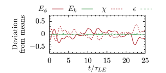
For reference, time series of kinetic energy, scalar variance and their respective dissipation rates

$$E_{k}\equiv\frac{1}{2}\langle\mathbf{u}\cdot\mathbf{u}\rangle,\quad E_{\phi}\equiv\frac{1}{2}\langle\phi^{2}\rangle,\quad\epsilon\equiv\nu\langle\nabla\mathbf{u}:\nabla\mathbf{u}\rangle,\quad\chi\equiv\kappa\langle\nabla\phi\cdot\nabla\phi\rangle,\quad\quad,$$

where the notation $\langle\cdot\rangle$ denotes a spatial average, for the DNS solution are shown in figure 1. The timescales considered ensure sufficient sampling of the temporal deviations from mean statistics (cf. Rao & de Bruyn Kops, 2011; Portwood et al., 2019a).

We optimise the coefficients in the $\mathbf{q}_{\text{PRS}}$ model and trainable parameters in the neural network $\mathbf{q}_{\text{ANN}}$ model for four filter length scales. Optimisation is performed by using training data obtained by filtering DNS solutions with (3), then calculating ground-truth $\mathbf{q}_{DNS}$ with (5). We note that optimisation of deterministic LES models with instantaneous a-priori filtered quantities is not strictly consistent with the sub-filter dynamics in actual a-posteriori simulation (Clark et al., 1979; Meneveau, 1994; Langford & Moser, 1999). While the approach will be shown to be valid in successive sections for resolved scalar dynamics of the stationary homogeneous isotropic flows considered here, we are cautious about generalising the approach to more complex flow configurations.

The selection of filter length scales are summarised in table 1, where $L_{f}$ is the outer length scale imposed by the forcing scheme, turbulent length scales are defined the standard way with

$$L_{k}=\left(\frac{\nu^{3}}{\epsilon}\right)^{1/4},\quad L_{E}=\frac{E_{k}^{3/2}}{\epsilon}$$ (10)

and where the filter scale is relative to the DNS grid spacing as

$$\Delta^{\ast}\equiv\Delta/\Delta_{\text{DNS}}\quad.$$ (11)

$\Delta^{\ast}$	$\Delta/L_{K}$	$\Delta/L_{E}$	$\Delta/L_{f}$
18	84	0.15	0.28
10	47	0.086	0.16
5.7	27	0.048	0.088
3.2	15	0.027	0.049

[table]A table beside a figure

Figure 1: Left, the time series of kinetic energy, scalar variance and their respective dissipation rates for the training dataset. Right, configuration of LES filter scales. A value of $\Delta^{\ast}=1$ indicates DNS resolution. Forcing is applied to the velocity field from largest scales in the domain until the smallest scale $L_{f}$.

With spatio-temporal sampling at large eddy scales, the reference DNS data yielded a total of 450,000 samples, with 20% of the data held out for out-of-sample testing. The deep feed-forward ANN consisted of 8 non-linear layers with ‘relu’ activation, 64 neurons per layer and a final linear layer with 512 neurons before the output layer $\mathbf{q}$ to yield a total of 65,000 trainable parameters. This architecture was observed to perform well with respect to different a-priori diagnostics in a hyper-parameter study. However, we do not dwell on other architectures since finding optimal architecture is not the objective of this study. Indeed, non-local approaches to neural network models have been suggested in recent literature (for instance Pawar et al., 2020; Yuan et al., 2020; Maulik & San, 2017). Such non-local neural network models may benefit from exploiting multi-point correlations in resolved flow parameters and may be analogous to non-local mathematical models, such as deconvolutional LES models (see Stolz & Adams, 1999, for instance).

We use the Adam optimiser to optimise the weights and biases of the $\mathbf{q}_{\text{ANN}}$ models with respect to the mean-squared-error (MSE) loss function $\mathcal{L}=E[(\mathbf{q}-\mathbf{q}_{\text{DNS}})^{2}]$. The optimiser iteratively modifies the weights and biases by using gradient descent with added momentum and dampening heuristics (Kingma & Ba, 2014). Training the ANN, first over 2000 iterations with a learning rate $\alpha=10^{-3}$ and then in a second stage over a similar number of iterations but with the learning rate decimated by an order of magnitude, was found to be robust. The loss function, normalised by the variance of $\mathbf{q}_{\text{DNS}}$ for the finest filter width, is shown for the training and testing sets in figure 2a.

Figure 2: Training and testing loss for each filter scale as a function of gradient descent iteration is shown in panel (a), where curves with decreasing losses correspond the finer filter scales. Central moments of the output parameter ${q_{z}}$, normalised by ground-truth data, for $\Delta^{\ast}=10$ as a function of gradient descent iteration is shown in panel (b). Note that the mean of ${q_{z}}$ develops much faster than higher-order moments.

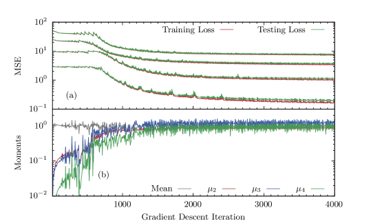
We observe the loss function remaining approximately flat for each case for the first 700 iterations. We show central moments of $q_{z}$, where the $i$-th moment is defined $\mu_{i}$, normalised by their ground-truth values as a function of gradient descent iteration in figure 2b. During this initial training period, we observe the mean value to converge within the first few iterations. However, successively higher central moments demonstrate a strong transient during this period. Most notably, $\mu_{4}$ does not converge until 1500 iterations. The convergence of these moments coincide with a decreasing rate-of-change of the loss function.

Finally, we note that in the PRS model, the constant $(C_{s})^{2}/Pr_{t}$ was similarly optimised using the same training data and loss function. The bulk constant is shown in figure 3a as a function of filter width. We observe some slight dependence of $(C_{s})^{2}/Pr_{t}$ on filter width $\Delta^{\ast}$.

Figure 3: (a) Optimised coefficients for the PRS model as a function of filter width, demonstrating mild anomalous scaling from $\Delta^{2}$. (b) Mean-squared-error of $\mathbf{q}$ for each model, normalised by the variance of $\mathbf{q}_{\text{DNS}}$ for each filter width.

Furthermore, the mean-squared-error of the two optimised models and the SAG model (which lacks any unknown coefficients) are shown in figure 3b. With respect to the ground-truth $\mathbf{q}_{\text{DNS}}$ variance, we observe the MSE of the PRS model to remain constant as a function of filter width. The ANN and SAG models exhibit strong dependence on $\Delta^{\ast}$, with the ANN model robustly out-performing the SAG model at coarsest filter widths and an approximately linear dependence on $\Delta^{\ast}$ when the filter width is small.

3 a-priori analysis

A useful a-priori characterisation of an LES model is its ability to reproduce the probability distribution function (p.d.f.) of the subfilter scale production of scalar variance, $\bar{P}_{\phi}$ as seen in the fully resolved computations, where the production is given by

$$\bar{P}_{\phi}=\mathbf{q}\cdot\nabla\bar{\phi}\quad.$$ (12)

The net downscale cascade of scalar variance in the setting considered, that is, a transfer from resolved scales to unresolved scales, leads to its mean value being positive.

The p.d.f. of the production of scalar variance is shown for the filtered DNS data and the three closures considered at all filter sizes in figures 4a-d, with the computation using testing set data.

Figure 4: A-priori comparison of the p.d.f.s of modelled and ground-truth production, normalised by ground-truth production standard deviation, log-scales inset. Note that forward- and back-scatter are more accurately captured by the ANN models. Also, note the apparent convergence of the SAG model to the ANN model and explicitly-filtered DNS results at the finest filter width in panel (d).

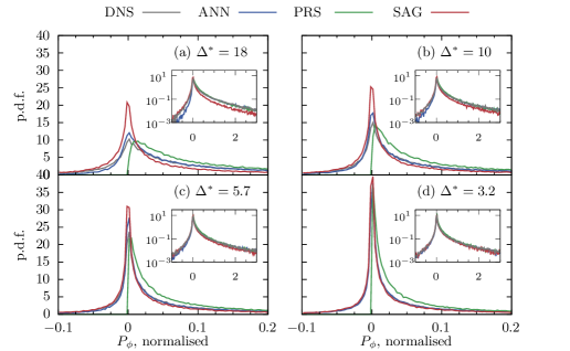
In this figure, the down-gradient nature of the residual flux in the PRS model constrains the production to be positive-definite whereas production in the DNS is not seen to be constrained in such a fashion. Indeed, the SAG model is seen to be able to produce counter-gradient fluxes (negative production) like in the reference DNS data. The ANN model is seen to similarly produces both counter-gradient and down-gradient fluxes. However, as mentioned earlier, that the SAG model tends to be under-dissipative is seen from the fact that the integrated value $E[\bar{P}_{\phi}]$ has a relative error of -56% at the coarsest filter scale, and -22% at the finest filter scale considered. The corresponding numbers for the PRS and ANN models are (0.19%, 4.2%) and (-1.5%, -0.12%) respectively. The ANN model is thus seen to exhibit advantageous characteristics by accurately capturing both mean dynamics of the subfilter scalar variance transfer rate, which in unenforced in optimisation procedure, and also the distribution of the transfer rate.

4 a-posteriori analysis

In an LES setting that models subfilter stresses in the momentum equation as well (that is, in addition to the subfilter scalar flux), dynamics of the passive scalar are affected not only by the model for the residual scalar flux, but also by the model for the residual momentum stress. It is easy to imagine parameter regimes where the indirect effects of the latter dominates the direct effects of the former, as far as the dynamics of the scalar are concerned. Therefore, in an effort to isolate the fundamental issue of scalar closure, we simulate the filtered passive scalar with exact advective coupling via explicit filtering of DNS solutions (1) (c.f. Vollant et al., 2016).

The three closure models are implemented in an a-posteriori simulation fashion and run for 5 large-eddy times using explicitly filtered DNS solution, not used in testing or training datasets, as initial conditions. The scalar variance for each model, $\langle\bar{\phi}^{2}\rangle/2$, is shown in figure 5a-d at four filter scales, each normalised by scalar variances obtained by explicitly filtering DNS solutions of the scalar. Visualisations of the evolution of scalars are included in Movie 1 of the accompanying supplementary material.

Figure 5: (a-d) Time series of relative error, with respect to filtered DNS solutions, of scalar variance $\langle\bar{\phi}^{2}\rangle$ at multiple filter scales. The finest filter is shown is panel (d), which demonstrates good performance for all models, while the ANN model features errors consistently an order of magnitude smaller than PRS and SAG models. Panels (e-h) indicate time series of local MSE of the scalar concentration, normalised by flux variance. Note the strong improvement of the SAG model with decreasing filter scale.

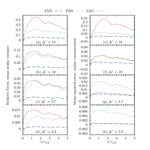
For the coarsest filter, shown in figure 5a, the SAG model characteristically under-dissipates and scalar variance diverges from the filtered DNS solution at early time. The optimal PRS model initially tracks the filtered DNS solution before $t/\tau_{LE}\approx 0.1$. For both the PRS and SAG models, the these the relative errors in resolved scalar variance soon begins to asymptote at large values. Whereas the large timescale trends in the evolution of filtered scalar variance is follow by all models, the SAG and PRS model over-predict scalar variance by 25% and 16%, respectively, after 5 large-eddy turnover times. The ANN model, however, tracks the filtered DNS solution accurately where the scalar variance after 5 large-eddy turnover times after is within 4.7% of the filtered DNS solution. The same general trend are observed in figure 5b where $\Delta^{\ast}=10$. The accuracy of the ANN model for $\Delta^{\ast}=18$ is only matched in PRS and SAG models for $\Delta^{\ast}=5.7$ as shown in figure 5c. When the filter length is small, all models track the filtered DNS solution well in time as shown in figure 5d as would be expected.

In addition to temporally tracking the evolution of mean scalar variance, spatio-temporally local metrics of the scalar concentration field are also important to consider for evaluation of a residual flux model. The evolution of mean-squared-error of the turbulence passive scalar concentrations, each normalised by scalar variances obtained by explicitly filtering DNS solutions, are shown in figures 5e-h. We observe broadly similar phenomenology compared to the evolution of scalar variances for PRS and ANN models across all filter widths – with the ANN model featuring an order of magnitude smaller local error than the PRS model over time for all filter widths. As the filter length scale decreases, we observe the SAG model to approach local errors that are very small with respect to the mean scalar variance, as is most evident in figure 5h. Indeed local errors become comparable to the ANN model at the smallest filter length scale, consistent with the observations that the a-priori subfilter scalar variance production recovers the distributions of the ground truth production at the finest filter scale for both ANN and SAG models, as previously discussed in figure 4d.

The temporal tracking of scalar concentration and variance is an interesting metric for evaluation of the ANN model because the model is developed without temporal correlations. The model also only depends on spatially-local quantities such that reconstruction of multi-point statistics may only be accurate if the structure of the ANN model accurately predicts the residual flux $\mathbf{q}$, i.e. it does not mimic dynamics in a purely functional sense. We evaluate two physically relevant multi-point diagnostics in figure 6.

Figure 6: Two-point diagnostics. (a-d) Second-order structure functions of resolved scalar in $z$, normalised by filtered DNS ground-truth data for each filter length. (e-h) Third-order structure functions in $z$ for the same filters length scales, normalised by ground-truth calculations using filtered DNS.

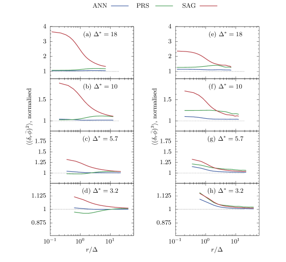
The second-order structure function of the scalar in the direction of the mean scalar gradient, normalised by the filtered DNS solution, after 5 large-eddy turnover times is shown in figures 6a-d for all filter scales. For all $\Delta^{\ast}$, the SAG model notably misses small-scale behaviour of the scalar, where the PRS and ANN models exhibit more similarity with the filtered DNS results. Except for the finest filter width, show in 6d, the PRS model begins to diverge at larger scales. The ANN model performs comparably for both filter scales presented and the diverging behaviour of the SAG at small scales is exaggerated with respect to the case with $\Delta^{\ast}=10$.

Higher order structure functions are also instructive. In passive scalar turbulence forced with a mean gradient, the third-order vertical structure function of the scalar is a physically-relevant diagnostic which should be preserved in a physically-accurate subfilter model (Warhaft, 2000). Third-order scalar structure functions are shown in figure 6e-h for all filter scales, each have been normalised by the values obtained from calculations using the filtered DNS solutions. First, we note that whereas the PRS model exhibits behaviour similar to that of the ANN model in the second-order structure functions, the same trends are not observed in figure 6e-h, especially at larger scales. The SAG model exhibits poorer consistency with large and small scales in 6e,f. Whereas the ANN model has some inconsistency with the DNS data at small scales, these errors are smaller than as observed in other models, and it closely follows the DNS results at larger scales. Similar behaviour is observed for $\Delta^{\ast}=18$ in figure 6e, except that errors may be more exaggerated at smaller scales for SAG and PRS models. The ANN model for this case exhibits some positive bias, almost uniformly for all $r/\Delta$.

5 Interpretation of data-driven models

We propose that it is instructive to consider the sensitivity of the residual flux to the input fields of scalar and velocity gradients as a means to get further insight into the learnt closure. Indeed, the automatic differentiation capability of the computational frameworks for developing ANNs, which are necessary for the optimisation of the networks via backpropagation, can be leveraged for such a study of the sensitivity of the residual flux to the input parameters. This type of differential sensitivity analysis provides phenomenological interpretability of neural network mappings, but falls short of determining causality (Gilpin et al., 2018), as would be apparent from models obtained by symbolic approaches (for instance Brunton et al., 2016).

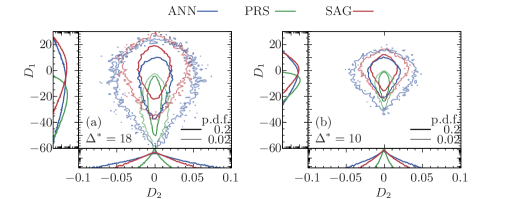
We compute such sensitivities with the test data and compare them against those for the ANN, PRS and SAG models. In particular, we present an analysis that considers

$$D_{1}\equiv\frac{\partial q_{z}}{\partial[\partial\bar{\phi}/\partial z]}\;\text{ and}\;D_{2}\equiv\frac{\partial q_{z}}{\partial[\partial\bar{u}_{z}/\partial x]}.$$ (13)

Isosurfaces of the joint pdf of (13) are shown in figure 7a for $\Delta^{\ast}=18$. At large $D_{1}$, the ANN model exhibits more similarity to the SAG model in terms of $D_{2}$. However, at moderate negative $D_{1}$, the model behaves more similar to the PRS model, particularly in the regions near $D_{2}\approx 0$. For the next finer filter scale with $\Delta^{\ast}=10$, as shown in figure 7b, isosurfaces of the gradients of the ANN model appear more similar to the SAG model. The interpretation of the ANN model being ‘intermediate’ of the SAG and PRS models suggests that perhaps the ANN model may be approximated by a mixed gradient models, wherein functional gradient diffusion is added to the structural gradient model. Furthermore, the ANN model increasingly mimics the SAG model with decreasing $\Delta^{\ast}$. The trend with $\Delta^{\ast}$ is consistent with the assumption of asymptotically small filter scale with the the SAG model, and suggests that the neural network learns to compensate with gradient-diffusion type dynamics as the filter scale is increased.

Figure 7: (a,b) joint p.d.f.s of the derivative of the vertical residual flux with respect to the vertical scalar gradient ($D_{1}$) and with respect to the horizontal derivative of vertical velocity ($D_{2}$). Note that the distribution of the ANN and SAG models become more similar with decreasing filter scale.

6 Concluding remarks

Encouraged by recent advancements of deep learning to industrial and technological applications, data-driven deep learning models have emerged as a promising route to calibrate, augment or replace existing models in the context of fluid turbulence. In addition to certification of model generalisation, which was not directly considered in this study, a major criticism of such learnt turbulence models is that they act as black-boxes, often impeding robust model certification. Responses to this criticism have ranged from attempts to incorporate physical or theoretical constraints, to imposing statistical symmetries, etc. either directly in the architecture of ANNs or through the loss function (Raissi et al., 2017). Surprisingly, a point of view that has not received much attention is that appropriately designed and trained ANNs will learn the correct structure of the closure, and that it remains to be interpreted and understood through proper analysis.

We have approached this point of view by the consideration of spatiotemporally local algebraic residual flux models. By reconstructing the residual fluxes from resolved parameters, we demonstrate the capability of neural networks to discover structural relations within the data without typical assumptions of scale similarity or asymptotically small filter scale. In training these ANN models, we interpret the training process from a statistical perspective by demonstrating that higher-order moments of model outputs require significantly more gradient-descent iterations to converge compared to the means. We are able to show that in addition to providing effective and competitive closures, when analysed in terms of dynamics and physically-relevant diagnostics, the learnt ANN model can indeed be interpreted in a physically and dynamically meaningful fashion. While not determining explicit causality, such an analysis permits us to demonstrate that the ANN appears to learn a closure which features dynamics reminiscent of both structural and functional LES closures (cf. mixed models). This in effect highlights the potential of machine learning in not only providing useful insights in the on-going task of developing and improving closures, but accelerating the process of model discovery.

7 Acknowledgements

The research activities of all authors are supported by a Laboratory Directed Research & Development (LDRD) project entitled “Machine Learning for Turbulence (MELT)” (20180059DR). This document has been approved for unlimited release from Los Alamos National Laboratory as LA-UR-20-20405.

References

- Balarac et al. (2013) Balarac, G., Le Sommer, J., Meunier, X. & Vollant, A. 2013 A dynamic regularized gradient model of the subgrid-scale scalar flux for large eddy simulations. Physics of Fluids 25 (7), 075107.
- Bardina et al. (1980) Bardina, J., Ferziger, J. H. & Reynolds, W. C. 1980 Improved subgrid scale models for large eddy simulations. Paper. AIAA.
- Beck et al. (2019) Beck, A., Flad, D. & Munz, C.-D. 2019 Deep neural networks for data-driven les closure models. Journal of Computational Physics 398, 108910.
- Brunton et al. (2020) Brunton, S. L., Noack, B. R. & Koumoutsakos, P. 2020 Machine learning for fluid mechanics. Annual Review of Fluid Mechanics 52 (1), 477–508.
- Brunton et al. (2016) Brunton, S. L., Proctor, J. L. & Kutz, J. N. 2016 Discovering governing equations from data by sparse identification of nonlinear dynamical systems. Proceedings of the national academy of sciences 113 (15), 3932–3937.
- Clark et al. (1979) Clark, R. A., Ferziger, J. H. & Reynolds, W. C. 1979 Evaluation of subgrid-scale models using an accurately simulated turbulent flow. J. Fluid Mech. 91, 1–16.
- Cybenko (1989) Cybenko, G. 1989 Approximation by superpositions of a sigmoidal function. Mathematics of Control, Signals and Systems 2 (4), 303–314.
- Daniel et al. (2018) Daniel, D., Livescu, D. & Ryu, J. 2018 Reaction analogy based forcing for incompressible scalar turbulence. Phys. Rev. Fluids 3, 094602.
- Gamahara & Hattori (2017) Gamahara, M. & Hattori, Y. 2017 Searching for turbulence models by artificial neural network. Phys. Rev. Fluids 2, 054604.
- Gilpin et al. (2018) Gilpin, L. H., Bau, D., Yuan, B. Z., Bajwa, A., Specter, M. & Kagal, L. 2018 Explaining explanations: An overview of interpretability of machine learning.
- Kingma & Ba (2014) Kingma, D. P. & Ba, J. 2014 Adam: A method for stochastic optimization.
- Kutz (2017) Kutz, J. N. 2017 Deep learning in fluid dynamics. Journal of Fluid Mechanics 814, 1–4.
- Langford & Moser (1999) Langford, J. A. & Moser, R. D. 1999 Optimal LES formulations for isotropic turbulence. J. Fluid Mech. 398, 321–346.
- Leonard (1974) Leonard, A. 1974 Energy cascade in LES of turbulent fluid flows. Ag 18A, 237–248.
- Ling et al. (2016) Ling, J., Kurzawski, A. & Templeton, J. 2016 Reynolds averaged turbulence modelling using deep neural networks with embedded invariance. Journal of Fluid Mechanics 807.
- Lu & Porté-Agel (2013) Lu, H. & Porté-Agel, F. 2013 A modulated gradient model for scalar transport in large-eddy simulation of the atmospheric boundary layer. Physics of Fluids 25 (1), 015110.
- Maulik & San (2017) Maulik, R. & San, O. 2017 A neural network approach for the blind deconvolution of turbulent flows. Journal of Fluid Mechanics 831, 151–181.
- Maulik et al. (2019a) Maulik, R., San, O., Jacob, J. D. & Crick, C. 2019a Sub-grid scale model classification and blending through deep learning. Journal of Fluid Mechanics 870, 784–812.
- Maulik et al. (2019b) Maulik, R., San, O., Rasheed, A. & Vedula, P. 2019b Subgrid modelling for two-dimensional turbulence using neural networks. Journal of Fluid Mechanics 858, 122–144.
- Meneveau (1994) Meneveau, C. 1994 Statistics of turbulence subgrid‐scale stresses: Necessary conditions and experimental tests. Physics of Fluids 6 (2), 815–833.
- Moghaddam & Sadaghiyani (2018) Moghaddam, A. A. & Sadaghiyani, A. 2018 A deep learning framework for turbulence modeling using data assimilation and feature extraction. arXiv preprint arXiv:1802.06106 .
- Nikolaou et al. (2019) Nikolaou, Z. M., Chrysostomou, C., Minamoto, Y. & Vervisch, L. 2019 Neural network-based modelling of unresolved stresses in a turbulent reacting flow with mean shear .
- Overholt & Pope (1996) Overholt, M. R. & Pope, S. B. 1996 Direct numerical simulation of a passive scalar with imposed mean gradient in isotropic turbulence. Phys. Fluids 8, 3128–3148.
- Overholt & Pope (1998) Overholt, M. R. & Pope, S. B. 1998 A deterministic forcing scheme for direct numerical simulations of turbulence. Computers & Fluids 27, 11–28.
- Pawar et al. (2020) Pawar, S., San, O., Rasheed, A. & Vedula, P. 2020 A priori analysis on deep learning of subgrid-scale parameterizations for kraichnan turbulence. Theoretical and Computational Fluid Dynamics .
- Portwood et al. (2019a) Portwood, G., de Bruyn Kops, S. & Caulfield, C. 2019a Asymptotic dynamics of high dynamic range stratified turbulence. Physical review letters 122 (19), 194504.
- Portwood et al. (2019b) Portwood, G. D., , Mitra, P. P., Ribeiro, M. D., Nguyen, T. M., Nadiga, B. T., Saenz, J. A., Chertkov, M., Garg, A., Anandkumar, A., Dengel, A. et al. 2019b Turbulence forecasting via Neural ODE. arXiv:1911.05180 .
- Raissi et al. (2017) Raissi, M., Perdikaris, P. & Karniadakis, G. E. 2017 Physics informed deep learning (part i): Data-driven solutions of nonlinear partial differential equations.
- Rao & de Bruyn Kops (2011) Rao, K. J. & de Bruyn Kops, S. M. 2011 A mathematical framework for forcing turbulence applied to horizontally homogeneous stratified flow. Phys. Fluids 23, 065110.
- Sagaut (2006) Sagaut, P. 2006 Large Eddy Simulation for Incompressible Flows, 3rd edn. Berlin: Springer.
- Salehipour & Peltier (2019) Salehipour, H. & Peltier, W. R. 2019 Deep learning of mixing by two ‘atoms’ of stratified turbulence. Journal of Fluid Mechanics 861, R4.
- Sarghini et al. (2003) Sarghini, F., De Felice, G. & Santini, S. 2003 Neural networks based subgrid scale modeling in large eddy simulations. Computers & fluids 32 (1), 97–108.
- Shete & de Bruyn Kops (2019) Shete, K. P. & de Bruyn Kops, S. M. 2019 Area of scalar isosurfaces in homogeneous isotropic turbulence as a function of reynolds and schmidt numbers. Journal of Fluid Mechanics 883.
- Smagorinsky (1963) Smagorinsky, J. 1963 General circulation experiments with the primitive equations. I. The basic experiment. Mon. Weather Rev. 91, 99–164.
- Speziale (1985) Speziale, C. G. 1985 Galilean invariance of subgrid-scale stress models in the large-eddy simulation of turbulence. J. Fluid Mech. 156, 55–62.
- Stolz & Adams (1999) Stolz, S. & Adams, N. A. 1999 An approximate deconvolution procedure for large-eddy simulation. Physics of Fluids 11 (7), 1699–1701.
- Vollant et al. (2016) Vollant, A., Balarac, G. & Corre, C. 2016 A dynamic regularized gradient model of the subgrid-scale stress tensor for large-eddy simulation. Physics of Fluids 28, 025114.
- Warhaft (2000) Warhaft, Z. 2000 Passive scalar in turbulent flows. Annu. Rev. Fluid Mech. 32, 203–240.
- Yuan et al. (2020) Yuan, Z., Xie, C. & Wang, J. 2020 Deconvolutional artificial neural network models for large eddy simulation of turbulence.