NICER–NuSTAR Observations of the Neutron Star Low-Mass X-ray Binary 4U 1735$-$44

Abstract

We report on the first simultaneous NICER and NuSTAR observations of the neutron star (NS) low-mass X-ray binary 4U 1735$-$44, obtained in 2018 August. The source was at a luminosity of $\sim 1.8~{}(D/5.6\ \mathrm{kpc})^{2}\times 10^{37}$ ergs s^-1 in the $0.4-30$ keV band. We account for the continuum emission with two different continuum descriptions that have been used to model the source previously. Despite the choice in continuum model, the combined passband reveals a broad Fe K line indicative of reflection in the spectrum. In order to account for the reflection spectrum we utilize a modified version of the reflection model relxill that is tailored for thermal emission from accreting NSs. Alternatively, we also use the reflection convolution model of rfxconv to model the reflected emission that would arise from a Comptonized thermal component for comparison. We determine that the innermost region of the accretion disk extends close to the innermost stable circular orbit ($R_{\mathrm{ISCO}}$) at the 90% confidence level regardless of reflection model. Moreover, the current flux calibration of NICER is within 5% of the NuSTAR/FPMA(B).

1 Introduction

4U 1735$-$44 is a low-mass X-ray binary (LMXB) located $5.6_{-2.1}^{+3.7}$ kpc away (Bailer-Jones et al., 2018) accreting via Roche-lobe overflow from a companion star of $\sim 1$ $M_{\odot}$. Type-I X-ray bursts were first observed in this system in 1985 with EXOSAT (van Paradijs et al., 1988), which positively identified the compact object as a neutron star (NS). The system has a mass function of $f(M)=0.53\pm 0.44$ $M_{\odot}$ and binary mass ratio of $q=0.05-0.41$ measured from radial velocity curves of Bowen fluorescence lines generated by X-ray irradiation of the companion star by the NS (Casares et al., 2006). 4U 1735$-$44 has an orbital period of $4.564\pm 0.005$ hours (Corbet et al., 1989) and is classified as an “atoll” source based on the island-like tracks the source traces out on color-color diagrams (Hasinger & van der Klis, 1989).

In many LMXBs, hard X-rays illuminating the accretion disk are reprocessed and reemitted in what is known as the reflection spectrum. The reprocessed continuum emission has a series of atomic features superimposed. These intrinsically narrow emission lines are broadened by special, Doppler, and general relativistic effects (Fabian et al., 1989). The strongest of these features is the Fe K line between $6.40-6.97$ keV. Spectral modeling of these broad reflection features are therefore used to determine properties of the NS, such as magnetic field strength (Cackett et al., 2009b; Ludlam et al., 2017c), probing the boundary layer region (King et al., 2016; Ludlam et al., 2019), or determining the radial extent of the compact object (Miller et al., 2013; Ludlam et al., 2017a).

The reflection spectrum of 4U 1735$-$44 has been studied previously using observations taken with Chandra, RXTE, XMM-Newton, and BeppoSAX (Cackett et al., 2009a; Torrejón et al., 2010; Ng et al., 2010; Mück et al., 2013). Simultaneous RXTE and Chandra observations were performed twice as part of a larger survey to investigate Fe lines in NS LMXBs (Cackett et al., 2009a). Though the Chandra gratings observations of the source did not show a clear Fe K line (Cackett et al., 2009a; Torrejón et al., 2010), the presence of a faint emission feature was not ruled out. An upper limit on the equivalent width of the Fe K line was placed at $<39.6$ eV (Cackett et al., 2009a). Later observations with XMM-Newton and BeppoSAX, however showed a broad Fe line with an equivalent width between $30-56$ eV (Ng et al., 2010; Mück et al., 2013), which is consistent with the upper limit from Chandra. 4U 1735$-$44 was at a similar flux level and spectral state in these different studies, so discrepancy between detection and non-detection can likely be attributed to a difference in collecting area between missions.

The Nuclear Spectroscopic Telescope Array (NuSTAR: Harrison et al. 2013) has provided an unhindered view of the reflection spectrum of a number of accreting NS systems (see Ludlam et al. 2019 and references therein) from $3-79$ keV. The individual pixel readout of the detectors makes NuSTAR an ideal mission with which to observe these bright accreting binary systems devoid of pile-up effects that impact CCD-based missions. The recent installation of the Neutron Star Interior Composition Explorer (NICER: Gendreau et al. 2012) on the International Space Station is a natural complement to NuSTAR with its 52 operational X-ray concentrator and silicon drift detector pairs that provide a large collecting area ($\sim 1800$ cm² at 1.5 keV) in the $0.2-12$ keV energy band and an energy resolution of $\sim 140$ eV at 6 keV. We obtained simultaneous observations of 4U 1735$-$44 with NICER and NuSTAR during 2018 August to investigate the reflection features in the combined X-ray passband. We present the observations and data reduction in §2, the analysis and results in §3, and conclude in §4.

2 Observations and Data Reduction

NuSTAR observed 4U 1735$-$44 on 2018 August 9 starting at 21:56:09 UT. ObsID 30363003002 contains 17.6 ks of data from Focal Plane Module (FPM) A and 17.7 ks from FPMB. The NuSTAR data were reduced using the standard data reduction process with nustardas v1.8.0 and caldb 20190314. Spectra and light-curves are extracted using a 100^′′ radius centered on the source. Backgrounds were generated from a radial region 100^′′ away from the source. We binned the FPMA/B spectrum by a factor of 3 using grppha (Choudhury et al., 2017).

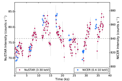
Figure 1: Light-curve for the NuSTAR/FPMA (circles) and NICER (stars) observations of 4U 1735$-$44 binned to 128 s. The grey dashed line indicates the average count rate for both NuSTAR and NICER. The time elapsed is from the start of the NuSTAR observation on 2018-08-09 at 21:56:09UT. The source exhibits $\leq 10\%$ variability over the course of the observation. Only one FPM is shown for clarity.

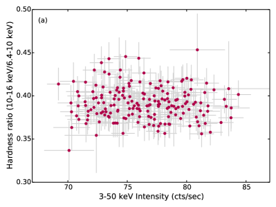
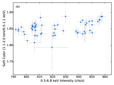
Figure 2: (a) NuSTAR hardness versus $3-50$ keV intensity diagram and (b) NICER soft color versus $0.5-6.8$ keV intensity diagram binned to 128 s. Although the source varies in intensity, the hardness ratio and soft color remains fairly constant. This indicates that variation in the continuum shape is minimal.

NICER observed 4U 1735$-$44 twice over the course of the NuSTAR observation. The first observation, ObsID 1050500103, began at 22:05:24 UT on 2018 August 9 for an exposure of 2.8 ks. The second observation, ObsID 1050500104, began at 00:00:52 UT on 2018 August 10 for 6.4 ks. The NICER observations were reduced using nicerdas 2019-06-19_V006a. Good time intervals (GTIs) were generated using nimaketime to select events that occurred when the particle background was low (KP $<$ 5 and COR_SAX $>$ 4) and avoiding times of extreme optical light loading (FPM_UNDERONLY_COUNT $<$ 200). GTIs were applied to the data selecting PI energy channels between 25 and 1200, inclusive, and EVENT_FLAGS=bxxx1x000 using niextract-events. See Bogdanov et al. (2019) for more information on the NICER screening flags. The resulting event files were loaded into xselect to extract a combined light-curve and spectrum. A background spectrum was generated following the same filtering criteria using RXTE “blank sky” field 5 (Jahoda et al., 2006). We use the standard public RMF and the on-axis average ARF available in CALDB release 20200202 when modeling the NICER spectrum.

No Type-I X-ray bursts were present in either data set, therefore no further processing was needed. Figure 1 shows the NuSTAR/FPMA (circles) and NICER (stars) light-curves binned to 128 s starting from when NuSTAR began observing 4U 1735$-$44. The source exhibits $\lesssim 10\%$ variability over the $\sim 40$ ks of elapsed time since the start of the observations. We check the NuSTAR hardness ratio ($10-16$ keV / $6.4-10$ keV: Coughenour et al. 2018) and NICER soft color ($1.1-2.0$ keV / $0.5-1.1$ keV: Bult et al. 2018) evolution of the source (Figure 2) and find that these remain fairly constant throughout the observation regardless of the change in intensity. This indicates that the spectral shape does not change dramatically during this time, hence we proceed with the analysis using the time averaged spectra that were extracted from the NICER and NuSTAR observations.

3 Analysis and Results

We use xspec v12.10.1f in our spectral analysis. NICER data are considered in the $0.4-10$ keV energy band, while NuSTAR is modeled in the $3-30$ keV range as the source spectrum becomes dominated by the background at higher energies. There are two high bins between $3.0-3.5$ keV in the NuSTAR/FPMA spectrum that are instrumental in origin, but still under investigation (K. K. Madsen, $priv.\ com.$). Since it is only present in the FPMA, we chose to leave these in the analysis rather than restricting the energy range further. To model the neutral absorption along the line of sight, we employ the xspec model tbabs (Wilms et al., 2000) with abundances set to wilm (Wilms et al., 2000) and vern cross-sections (Verner et al., 1996). There were still two narrow absorption features present in the low energy NICER spectrum. These may be astrophysical or due to the low absorption column and luminosity of the source revealing instrumental uncertainties within the spectrum since NICER’s calibration is still ongoing. We account for these features with two edge components. These occur at $\sim 0.5$ keV and $\sim 0.8$ keV, which corresponds to neutral O K and Fe L edges, respectively. These would be interstellar in origin if indeed they are astrophysical as opposed to instrumental. We allow a constant to float for the FPMB and NICER with respect to the FPMA (which is fixed at unity).

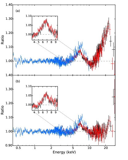
Figure 3: Ratio of the NICER (blue), NuSTAR/FPMA (black), and NuSTAR/FPMB (red) data to the simple continuum of (a) Model 1 and (b) Model 2. Note that the iron line region from $5–8$ keV and Compton hump region from $15-25$ keV were ignored while fitting the continuum to highlight these features and prevent them from skewing the fit shown here. The inset panel shows a close up of the NuSTAR Fe line profiles for each continuum description. A broad Fe K line is visible regardless of continuum choice, though the Compton hump is not as visible in panel (b) due to the high-energy rollover of the Comptonization model trying to characterize this component.

Table 1: Joint NICER and NuSTAR spectral modeling of 4U 1735$-$44

Component	Parameter	Model 1	Model 2	Model 3		Model 4
				(a) Free $A_{Fe}$	(b) Fixed $A_{Fe}$
Constant	$C_{\mathrm{FPMA}}$	1.0	1.0	1.0	1.0	1.0
	$C_{\mathrm{FPMB}}$	$0.996\pm 0.002$	$0.996\pm 0.002$	$0.995_{-0.003}^{+0.004}$	$0.996_{-0.008}^{+0.002}$	$0.996\pm 0.002$
	$C_{\mathrm{NICER}}$	$1.040\pm 0.003$	$1.039\pm 0.003$	$1.037\pm 0.003$	$1.036_{-0.013}^{+0.002}$	$1.037_{-0.002}^{+0.004}$
Tbabs	NH (1021 cm-2)	$4.91\pm 0.04$	$3.21\pm 0.02$	$4.69_{-0.04}^{+0.13}$	$4.8_{-0.2}^{+0.3}$	$3.2_{-0.02}^{+0.01}$
edge	E (keV)	$0.81\pm 0.01$	$0.86\pm 0.01$	$0.82_{-0.01}^{+0.02}$	$0.81_{-0.02}^{+0.01}$	$0.84\pm 0.01$
	$\tau_{\mathrm{max}}$	$0.123\pm 0.008$	$0.044\pm 0.006$	$0.058_{-0.003}^{+0.016}$	$0.05_{-0.01}^{+0.07}$	$0.09\pm 0.01$
edge	E (keV)	$0.526\pm 0.004$	$0.528\pm 0.005$	$0.522\pm 0.004$	$0.529_{-0.007}^{+0.002}$	$0.54\pm 0.01$
	$\tau_{\mathrm{max}}$	$0.23\pm 0.02$	$0.11\pm 0.02$	$0.19\pm 0.02$	$0.23_{-0.01}^{+0.04}$	$0.208_{-0.03}^{+0.02}$
bbody	$kT$ (keV)	$2.43\pm 0.02$	…	…	…	…
	normbb (10-2)	$1.02\pm 0.01$	…	…	…	…
diskbb	$kT$ (keV)	$1.26\pm 0.02$	$0.68\pm 0.01$	$1.04\pm 0.04$	$1.03_{-0.04}^{+0.02}$	$0.58_{-0.02}^{+0.01}$
	normdisk	$28_{-1}^{+2}$	$350_{-18}^{+25}$	$59_{-7}^{+4}$	$58_{-11}^{+5}$	$507_{-18}^{+38}$
powerlaw	$\Gamma$	$2.57\pm 0.02$	…	$2.73\pm 0.05$	$2.71_{-0.11}^{+0.06}$	…
	normpl	$0.45\pm 0.01$	…	$0.30\pm 0.04$	$0.33_{-0.03}^{+0.12}$	…
nthcomp	$\Gamma$	…	$1.97\pm 0.03$	…	…	$1.76\pm 0.01$
	$kT_{e}$ (keV)	…	$3.13\pm 0.04$	…	…	$2.87\pm 0.03$
	$kT_{bb}$ (keV)	…	$1.07_{-0.04}^{+0.03}$	…	…	$0.70\pm 0.03$
	normnth ($10^{-2}$)	…	$5.9_{-0.3}^{+0.4}$	…	…	$11.3_{-0.9}^{+1.1}$
relxillNS	$q$	…	…	$3.3_{-1.1}^{+0.2}$	$3.5_{-0.9}^{+0.3}$	…
	$i$ (∘)	…	…	$42_{-4}^{+2}$	$42_{-3}^{+2}$	…
	$R_{\rm in}$ (ISCO)	…	…	$1.01_{-0.01}^{+0.57}$	$1.01_{-0.01}^{+0.74}$	…
	$R_{\rm in}$ ($R_{g}$)	…	…	$6.06_{-0.06}^{+3.42}$	$6.06_{-0.06}^{+4.44}$	…
	$kT_{bb}$ (keV)	…	…	$2.89_{-0.03}^{+0.02}$	$2.86_{-0.07}^{+0.01}$	…
	$\log(\xi)$	…	…	$3.66_{-0.12}^{+0.06}$	$3.53_{-0.12}^{+0.04}$	…
	$A_{Fe}$	…	…	$4.24_{-0.7}^{+1.6}$	$2.0^{\dagger}$	…
	$\log(N)$ (cm-3)	…	…	$16.9_{-0.9}^{+0.4}$	$17.0_{-0.5}^{+0.4}$	…
	$f_{refl}$	…	…	$0.3\pm 0.2$	$0.3_{-0.2}^{+0.1}$	…
	normrel (10-3)	…	…	$1.6_{-0.5}^{+0.9}$	$1.7_{-0.3}^{+0.1}$	…
rdblur	Betor10	…	…	…	…	$-2.3_{-0.2}^{+0.1}$
	$R_{\rm in}$ ($R_{g}$)	…	…	…	…	$6.10_{-0.02}^{+9.25}$
	$i$ (∘)*	…	…	…	…	$57\pm 2$
rfxconv	$rel_{\mathrm{refl}}$	…	…	…	…	$0.19_{-0.02}^{+0.40}$
	$A_{Fe}$	…	…	…	…	$2.0_{-0.4}^{+0.5}$
	$\cos{(i)}$*	…	…	…	…	–
	$\log(\xi)$	…	…	…	…	$2.72_{-0.03}^{+0.05}$
	$\chi^{2}/dof$	3106.62/1394	2272.66/1394	1661.39/1387	1679.12/1388	1735.97/1388
${}^{\dagger}=\mathrm{fixed}$, $*=\mathrm{tied}$

Note.— Errors are given at the 90% confidence level. The input seed photon type in nthcomp is set to a single temperature blackbody (inp_type=0). The bbody normalization is defined as $(L/10^{39}\ \mathrm{erg\ s^{-1}})/(D/10\ \mathrm{kpc})^{2}$. The diskbb normalization is defined as $(R_{in}/\mathrm{km})^{2}/(D/10\ \mathrm{kpc})^{2}\times\cos{\theta}$. The power-law normalization is defined as photons keV^-1 cm⁻² s⁻¹ at 1 keV. The emissivity indices in relxillNS are tied to create a single emissivity index, $q$. The outer disk radius is fixed at a value of 990 $R_{g}$ (165 $R_{\mathrm{ISCO}}$) and the dimensionless spin parameter is set to $a=0$.

We fit the continuum with two models that have been previously used to describe the spectrum of 4U 1735$-$44. Cackett et al. (2009a) modeled the continuum with the three component model for accreting atolls as described in Lin et al. (2007): a single-temperature blackbody (bbody) for thermal emission from the NS or boundary layer, a multi-temperature blackbody (diskbb: Mitsuda et al. 1994) to model the accretion disk, and a power-law to account for weak Comptonization. We refer to this as Model 1 in Table 1. This model gives an accretion disk temperature of $kT=1.26\pm 0.02$ keV, single-temperature blackbody component of $kT=2.43\pm 0.02$ keV, and power-law index of $\Gamma=2.57\pm 0.02$. These are similar to the continuum parameters from Cackett et al. (2009a) when fitting the Chandra and RXTE observations.

Alternatively, Mück et al. (2013) described the BeppoSAX broad-band continuum with diskbb and a thermal Comptonization component (nthcomp: Zdziarski et al. 1996; Zycki et al. 1999). This is referred to as Model 2 in Table 1. This model returns a lower accretion disk temperature of $0.68\pm 0.01$ keV, photon index of $\Gamma=1.97\pm 0.03$, electron temperature of $kT_{e}=3.13\pm 0.04$ keV, and seed photon temperature of $kT_{bb}=1.07_{-0.04}^{+0.03}$ keV, which agree with the range values found in Mück et al. (2013). Regardless of the choice in continuum, the presence of reflection is clearly evident in the ratio of the data to each respective model (Figure 3), though the Compton hump at higher energies is less noticeable when using Model 2 due to the curvature of the high-energy rollover in nthcomp.

Previous treatments of the reflected emission in this source consisted of modeling a Gaussian emission line or diskline component to the Fe line between $6.40-6.97$ keV (Cackett et al., 2009a; Ng et al., 2010; Mück et al., 2013). Here, we model the entire reflection spectrum using the special flavor of relxill (García et al., 2014) that assumes a thermal input spectrum, $kT_{bb}$, from the surface or boundary layer of the NS (relxillNS) in contrast to a power-law, $\Gamma$, input of the standard model. This new model has similar parameters to relxill with the addition of a variable disk density component, $\log(N\mathrm{[cm^{-3}]})$. The other parameters of this model include an inner emissivity index ($q_{in}$), outer emissivity index ($q_{out}$), the break radius ($R_{break}$) between the two emissivity indices, dimensionless spin parameter ($a$), redshift ($z$), inclination of the system ($i$), inner disk radius ($R_{\rm in}$) in units of the innermost stable circular orbit (ISCO), outer disk radius ($R_{out}$) in units of gravitational radii ($R_{g}=GM/c^{2}$), ionization parameter ($\log(\xi)$), iron abundance ($A_{Fe}$), and reflection fraction ($f_{refl}$). We tie the inner and outer emissivity indices to create a single emissivity profile, $q$, making $R_{break}$ obsolete. $z=0$ since 4U 1735$-$44 is a Galactic source. The outer disk radius is set at 990 $R_{g}$ and the spin parameter is fixed at $a=0$ (Ludlam et al., 2018). We allow the reflection fraction, $f_{refl}$, to be positive so that it encompasses the single temperature blackbody from the continuum and reflection emission component. The results of using relxillNS can be found under Model 3 in Table 1.

Conversely, to model the reflected emission when using the continuum description of Model 2, we use the reflection convolution model rfxconv (Done & Gierliński, 2006; Kolehmainen et al., 2011). This generates an angle-dependent reflection spectrum from the nthcomp input spectrum by combining the reflection emission from an ionized disk interpolated from reflionx (Ross & Fabian, 2005) below 14 keV (using the average $2-10$ keV power-law index) with Compton reflected emission from pexriv (Magdziarz & Zdziarski, 1995) above 14 keV (using the average $12-14$ keV power-law index). The parameters of this model are the relative reflection normalization ($rel_{\mathrm{refl}}$), the Fe abundance ($A_{Fe}$), the inclination angle ($\cos{(i)}$), redshift ($z$), and ionization parameter ($\log(\xi)$). Additionally, we convolve rfxconv with the relativistic blurring kernal rdblur (Fabian et al., 1989) to take into account general and special relativistic effects around a non-spinning compact object (i.e., $a=0$). The parameters of rdblur are the emissivity index (Betor10: $R^{\mathrm{Betor10}}$), inner disk radius in $R_{g}$, outer disk radius, and inclination ($i$). The outer disk radius is fixed at 990 $R_{g}$ to be consistent with relxillNS. Moreover, we tie the inclination parameters between rdblur and rfxconv for consistency. This is referred to as Model 4 in Table 1.

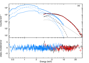
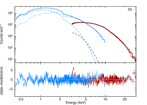
Figure 4: The NICER (blue), NuSTAR/FPMA (black), and NuSTAR/FPMB (red) spectra and model components for (a) Model 3 (free $A_{Fe}$) and (b) Model 4 with the square-root of $\chi^{2}$ in each bin shown in the lower panels. The dashed line indicates the multi-temperature accretion disk component. The solid line is the relxillNS component, which includes the single-temperature blackbody input spectrum. The dotted line shows the power-law component. The dot-dot-dot-dash line is the blurred reflection and Comptonized continuum from using rfxconv. We only show the model components for the NICER and NuSTAR/FPMA spectra for clarity.

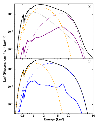
Figure 5: The unfolded model for (a) Model 3a and (b) Model 4. The solid black line indicates the overall model. The dashed orange line indicated the multi-temperature disk component in each model. The dotted grey line indicates the power-law component for Model 3a. The solid purple line in panel (a) represents the reflection component relxillNS while the dot-dashed line of the same color is the input blackbody continuum component. The solid blue line in panel (b) indicates the reflection spectrum using rfxconv and the dot-dashed line is the input Comptonization spectrum.

In each case, the addition of a reflection model improves the overall fit by $\geq 18\sigma$ (via an F-test) in comparison to their respective continuum model. The multiplicative constant is within 1% for the FPMB and within 5% for NICER relative to the FPMA. The improvement in the NICER response files are evident when compared to spectral modeling with the previous arf version nixtiaveonaxis20170601v002.arf (especially near the Au M edges; see Figure 1 of Ludlam et al. 2018). There is some discrepancy above 6 keV as can be seen in the differences in the blue-wing of the Fe line profile in Figure 3 and the lower panel of Figure 4. The reflection model fits between the difference in the shape of the Fe line profiles from NICER and NuSTAR. The discrepancy in this region is only at the few percent level, but can contribute to uncertainty on the inclination, $i$, position of the inner disk radius, $R_{\rm in}$, abundance of Fe, $A_{Fe}$, and disk density. It is unclear how much of this is due to NICER’s calibration, the difference in energy resolution between missions, or to the current understanding and methodology of modeling the NICER background. However, it is necessary to fit the NICER and NuSTAR data simultaneously. When modeling the NICER data alone, the power-law index in Model 1 is not well constrained without the higher energy photons that NuSTAR can provide. Additionally, the emissivity index is unconstrained regardless of the continuum description when omitting the NuSTAR data. On the other hand, the NuSTAR spectrum is unable to constrain the neutral absorption column along the line of sight without the addition of NICER’s low-energy passband.

The inferred neutral absorption column along the line of sight is slightly higher than the fixed value of $3.0\times 10^{21}$ cm^-2 that was used in Cackett et al. (2009a) and Mück et al. (2013). Model 3 has an emissivity index of $q=3.3_{-0.1}^{+0.2}$, inclination of $i=42_{-4}^{+2}$ ^∘, inner disk radius of $R_{\mathrm{in}}=1.01_{-0.01}^{+0.57}$ $R_{\mathrm{ISCO}}$, ionization of $\log(\xi)=3.66_{-0.12}^{+0.06}$, Fe abundance (relative to solar) of $A_{Fe}=4.24_{-0.7}^{+1.6}$, disk density of $\log(N)=16.9_{-0.9}^{+0.4}$, and reflection fraction of $f_{refl}=0.3\pm 0.2$. The $A_{Fe}$ is several times higher than solar, but this is well within the range for Fe abundance that was previously reported in Mück et al. (2013). To determine how this parameter impacts the values inferred from relxillNS, we fix it to a lower value of $A_{Fe}=2$. The resulting fit is $3.8\sigma$ worse than when $A_{Fe}$ was allowed to be a free parameter. However, the other parameters are all still consistent within the 90% confidence level. Therefore, the other parameters are not highly reliant upon $A_{Fe}$. We report this fit within Table 1 under Model 3 (b) fixed $A_{Fe}$ for direct comparison to Model 3 (a) free $A_{Fe}$.

Model 4 has an emissivity index of $-2.3_{-0.2}^{+0.1}$, inclination of $i=57\pm 2^{\circ}$, inner disk radius of $R_{\mathrm{in}}=6.10_{-0.02}^{+9.25}$ $R_{g}$, ionization of $\log(\xi)=2.72_{-0.03}^{+0.05}$, Fe abundance of $A_{Fe}=2.0_{-0.4}^{+0.5}$, and reflection fraction of $rel_{refl}=0.19_{-0.02}^{+0.40}$. The inner disk radius agrees within the 90% confidence level between Model 3 and 4, which indicates that the choice of continuum and reflection model does not significantly impact this result (also see Coughenour et al. 2018 and Ludlam et al. 2017a). The discrepancy between the other recovered parameters from these two models can be attributed to the many differences between the two approaches. This is particularly true for the inclination. While the model rdblur*rfxconv applies an outdated relativistic convolution routine to a reflection spectrum produced from piecing together two different reflection codes (reflionx and pexriv), relxillNS self-consistently connects the angle-dependent reflection spectrum (produced with a blackbody illumination in xillverNS) with the ray tracing code relline (Dauser et al., 2010). At each disk radius, the model chooses the appropriate reflection spectrum for each emission angle calculated in a curved space-time. The resulting reflection model thus accurately captures the detailed dependence of the emitted spectrum with the viewing angle (García et al., 2014; Dauser et al., 2014). Additionally, the disk density differs between these two models as Model 3 has a $\log(N)\sim 17$ and Model 4 has a hard-coded density of $\log(N)=15$. A more detailed description of relxillNS and comparison to other reflection models is forthcoming (García, Dauser, & Ludlam 2020, in preparation).

Figure 5 shows the unfolded model and components for Model 3a and Model 4. The shape of the resulting reflection spectrum is very different given that the model in panel (a) results from a blackbody input spectrum and panel (b) is pieced together from power-law and Comptonization inputs. There is a flavor of relxill where the input spectrum is a Comptonization component (relxillCP), but this assumes that the seed photons arise from a multi-temperature blackbody (inp_type=1 in nthcomp for the accretion disk) which is more appropriate for black hole systems. This differs from the single-temperature input type used here and would be an inconsistent treatment of the reflection component with respect to the illuminating continuum.

4 Conclusion

We report on the first simultaneous NICER and NuSTAR observations of the persistently accreting NS LMXB 4U 1735$-$44. Regardless of the choice in continuum modeling, there are clear signatures of reflection in the NICER and NuSTAR spectrum. Previous treatments of the reflection component in this system only modelled emission in the Fe line region. We model the entire reflection spectrum using the modified version of relxill that is tailored for thermal emission from a neutron star, relxillNS, and with the reflection convolution model rfxconv. The source was at an unabsorbed luminosity of $1.8\pm 1.1(D/5.6\ \mathrm{kpc})^{2}\times 10^{37}$ ergs s^-1 in the $0.4-30$ keV band, which is a similar luminosity as when it was observed with XMM-Newton, RXTE, Chandra, and BeppoSAX (Cackett et al., 2009a; Ng et al., 2010; Mück et al., 2013). This corresponds to $L/L_{\mathrm{Edd}}=0.05\pm 0.03(D/5.6\ \mathrm{kpc})^{2}$ assuming a maximum Eddington luminosity of $3.8\times 10^{38}$ ergs s^-1 (Kuulkers et al., 2003).

From the self-consistent relxillNS reflection modeling, we infer an inner disk radius of $R_{\mathrm{in}}=1.01_{-0.01}^{+0.57}$ $R_{\mathrm{ISCO}}$ (Model 3a). Under the assumption of $a=0$, this corresponds to $R_{\mathrm{in}}=6.06_{-0.06}^{+3.42}$ $R_{g}$ or $R_{\mathrm{in}}=12.52_{-0.12}^{+7.07}$ km when assuming a canonical NS mass of 1.4 $M_{\odot}$. Using the alternative continuum model with rfxconv (Model 4) provides a larger uncertainty in the inner disk radius, $R_{\mathrm{in}}=6.10_{-0.02}^{+9.25}$ $R_{g}$ $=12.61_{-0.04}^{+19.1}$ km, but is consistent within the 90% confidence level. The inner disk radius inferred from the normalization of diskbb gives a smaller but consistent range of $R_{\mathrm{in}}\sim 14-15$ km in the case of Model 3a, when using a correction factor of 1.7 (Shimura & Takahara, 1995), inclination of $44^{\circ}$, and $D=5.6$ kpc. The inner disk radius from diskbb is higher for Model 4, $R_{\mathrm{in}}\sim 48.5-51.2$ km, when using the same correction factor and distance, but higher inclination of $57^{\circ}$. The inclination of the system inferred from reflection modeling differs between model, $i=38^{\circ}-44^{\circ}$ for relxillNS and $i=55^{\circ}-59^{\circ}$ for rfxconv, but both agree with the estimation from optical spectroscopy ($i=27^{\circ}-60^{\circ}$: Casares et al. 2006). Unfortunately, the large uncertainty in the mass ratio of the system prevents our smaller range in inclination from placing meaningful constraints on the mass of the NS.

The upper limit on the unabsorbed luminosity of 4U 1735$-$44 (assuming $D=5.6$  kpc) can be used to place a limit on the radial extent of a boundary layer region between the inner edge of the accretion disk and surface of the NS by using equation (25) in Popham & Sunyaev (2001). The maximum extent of this region is $R_{BL}=6.1$ $R_{g}$. It is plausible that there is a boundary layer present in this system given that the inner disk radius is consistent with $R_{\mathrm{ISCO}}$. Conversely, we can also place an upper limit on the dipolar equatorial magnetic field strength of the NS from the upper limit on $R_{\rm in}$. Adapting equation (1) in Cackett et al. (2009b) for the magnetic dipole moment to directly provide the magnetic field strength, we obtain:

$$B=3.5\times 10^{5}\ k_{A}^{-7/4}\ x^{7/4}\left(\frac{M}{1.4\ M_{\odot}}\right)^{2}\left(\frac{10\ \mathrm{km}}{R_{NS}}\right)^{3}$$ (1)

$$\times\left(\frac{f_{ang}}{\eta}\frac{F_{bol}}{10^{-9}\ \mathrm{erg\ cm^{-2}\ s^{-1}}}\right)^{1/2}\frac{D}{3.5\ \mathrm{kpc}}\ \mathrm{G}$$

Assuming an accretion efficiency of $\eta=0.2$ (Sibgatullin & Sunyaev, 2009), unity for the conversion factor ($k_{A}$) and angular anisotropy ($f_{ang}$) as in Ludlam et al. (2019), a distance of 5.6 kpc, and conical values for NS mass and radius, we acquire an upper limit of $B\leq 2.0\times 10^{8}$ G from Model 3a and $B\leq 4.6\times 10^{8}$ G from Model 4. The magnetic field strength agrees with other accreting NS LMXBs (Mukherjee et al., 2015; Ludlam et al., 2017c).

The current flux calibration of NICER is within $5\%$ of the NuSTAR FPMA/B. Further improvements to the response files for NICER may bring the Fe band into complete agreement with NuSTAR, though the current discrepancy is only at the few percent level. However, it is clear that the combined passband of NICER and NuSTAR can reveal the entire reflection spectrum of these bright sources without the need to correct for pile-up effects.

Acknowledgements: R.M.L. thanks K. K. Madsen for discussion regarding instrumentation. Support for this work was provided by NASA through the NASA Hubble Fellowship grant #HST-HF2-51440.001 awarded by the Space Telescope Science Institute, which is operated by the Association of Universities for Research in Astronomy, Incorporated, under NASA contract NAS5-26555. J.A.G. acknowledges support from NASA grant 80NSSC19K1020 and from the Alexander von Humboldt Foundation. E.M.C. gratefully acknowledges support through NSF CAREER award number AST-1351222. C.M. is supported by an appointment to the NASA Postdoctoral Program at the MSFC, administered by USRA.

References

- Bailer-Jones et al. (2018) Bailer-Jones, C. A. L., Rybizki, J., Fouesneau, M., et al. 2018, AJ, 156, 58
- Bogdanov et al. (2019) Bogdanov, S., Guillot, S., Ray, P. S., et al. 2019, ApJL, 887, L25
- Bult et al. (2018) Bult, P., Altamirano, D., Arzoumanian, Z., et al. 2018, ApJL, 860, L9
- Cackett et al. (2009a) Cackett, E. M., Miller, J. M., Homan, J., et al. 2009, ApJ, 690, 1847
- Cackett et al. (2009b) Cackett, E. M., Altamirano, D., Patruno, A., et al. 2009, ApJ, 694, L21
- Casares et al. (2006) Casares, J., Cornelisse, R., Steeghs, D., et al. 2006, MNRAS, 373, 1235
- Choudhury et al. (2017) Choudhury, K., García, J. A., Steiner, J. F., & Bambi, C. 2017, ApJ, 851, 57
- Corbet et al. (1989) Corbet, R., Smale, A., Charles, P., et al. 1989, MNRAS, 239, 533
- Coughenour et al. (2018) Coughenour, B. M., Cackett, E. M., Miller, J. M., & Ludlam, R. M. 2018, ApJ, 867, 64
- Dauser et al. (2010) Dauser, T., Wilms, J., Reynolds, C. S., & Brenneman, L. W. 2010, MNRAS, 409, 1534
- Dauser et al. (2014) Dauser, T., García, J., Parker, M. L., Fabian, A. C., & Wilms, J. 2014, MNRAS, 444, L100
- Done & Gierliński (2006) Done, C., & Gierliński, M. 2006, MNRAS, 367, 659
- Fabian et al. (1989) Fabian, A. C., Rees, M. J., Stella, L., & White, N. E. 1989, MNRAS, 238, 729
- García et al. (2014) García, J., Dauser, T., Lohfink, A., et al. 2014, ApJ, 782, 76
- Gendreau et al. (2012) Gendreau, K. C., Arzoumanian, Z., & Okajima, T. 2012, Proc. SPIE, 8443, 13
- Harrison et al. (2013) Harrison, F. A., Craig, W. W., Christensen, F. E., et al. 2013, ApJ, 770, 103
- Hasinger & van der Klis (1989) Hasinger, G., & van der Klis, M. 1989, A&A, 225, 79
- Jahoda et al. (2006) Jahoda, K., Markwardt, C. B., Radeva, Y., et al. 2006, ApJS, 163, 401
- King et al. (2016) King, A. L., Tomsick, J. A., Miller, J. M., et al. 2016, ApJL, 819, L29
- Kolehmainen et al. (2011) Kolehmainen, M., Done, C., & Díaz Trigo, M. 2011, MNRAS, 416, 311
- Kuulkers et al. (2003) Kuulkers, E., den Hartog, P. R., in’t Zand, J. J. M., et al. 2003, A&A, 399, 663
- Lin et al. (2007) Lin, D., Remillard, R. A., & Homan, J. 2007, ApJ, 667, 1073
- Ludlam et al. (2017a) Ludlam, R. M., Miller, J. M., Bachetti, M., et al. 2017a, ApJ, 836, 140
- Ludlam et al. (2017c) Ludlam, R. M., Miller, J. M., Degenaar, N., et al. 2017c, ApJ, 847, 135
- Ludlam et al. (2018) Ludlam, R. M., Miller, J. M., Arzoumanian, Z., et al. 2018, ApJ, 858, L5
- Ludlam et al. (2019) Ludlam, R. M., Miller, J. M., Barret, D., et al. 2019, ApJ, 873, 99
- Magdziarz & Zdziarski (1995) Magdziarz, P., & Zdziarski, A. 1995, MNRAS, 273, 837
- Miller et al. (2013) Miller, J. M., Parker, M. L., Fuerst, F., et al. 2013, ApJL, 779, L2
- Mitsuda et al. (1994) Mitsuda, K., Inoue, H., Koyama, K., et al. 1984, PASJ, 36, 741
- Mück et al. (2013) Mück, B., Piraino, S., & Santangelo, A. 2013, A&A, 555, A17
- Mukherjee et al. (2015) Mukherjee, D., Bult, P., van der Klis, M., & Bhattacharya, D. 2015, MNRAS, 452, 3994
- Ng et al. (2010) Ng, C., Díaz Trigo, M., Cadolle Bel, M., & Migliari, S. 2010, A&A, 522, A96
- Popham & Sunyaev (2001) Popham, R., & Sunyaev, R. 2001, ApJ, 547, 355
- Ross & Fabian (2005) Ross, R. R., & Fabian, A. C. 2005, MNRAS, 358, 211
- Sibgatullin & Sunyaev (2009) Sibgatullin, N. R., & Sunyaev, R. A. 2000, AstL, 26, 699
- Shimura & Takahara (1995) Shimura, T., & Takahara, R. 1995, ApJ, 445, 780
- Torrejón et al. (2010) Torrejón, J. M., Schulz, N. S., Nowak, M. A., & Kallman, T. R. 2010, ApJ, 715, 947
- van Paradijs et al. (1988) van Paradijs, J., Penninx, W., Lewin, W. H. G., Sztajno, M., & Truemper, J. 1988, A&A, 192, 147
- Verner et al. (1996) Verner, D. A., Ferland, G. J., Korista, K. T., & Yakovlev, D. G. 1996, ApJ, 465, 487
- Wilms et al. (2000) Wilms, J., Allen, A., & McCray, R. 2000, ApJ, 542, 914
- Zdziarski et al. (1996) Zdziarski, A. A., Johnson, W. N., & Magdziarz, P. 1996, MNRAS, 283, 193
- Zycki et al. (1999) Zycki, P. T., Done, C., & Smith, D. A. 1999, MNRAS, 309, 561