Scalability of High-Performance PDE Solvers

Abstract

Performance tests and analyses are critical to effective HPC software development and are central components in the design and implementation of computational algorithms for achieving faster simulations on existing and future computing architectures for large-scale application problems. In this paper, we explore performance and space-time trade-offs for important compute-intensive kernels of large-scale numerical solvers for PDEs that govern a wide range of physical applications. We consider a sequence of PDE-motivated bake-off problems designed to establish best practices for efficient high-order simulations across a variety of codes and platforms. We measure peak performance (degrees of freedom per second) on a fixed number of nodes and identify effective code optimization strategies for each architecture. In addition to peak performance, we identify the minimum time to solution at 80% parallel efficiency. The performance analysis is based on spectral and $p$-type finite elements but is equally applicable to a broad spectrum of numerical PDE discretizations, including finite difference, finite volume, and $h$-type finite elements.

1 Introduction

One characteristic common to many science and engineering applications in high-performance computing (HPC) is their enormous range of spatial and temporal scales, which can manifest as billions of degrees of freedom (DOFs) to be updated over tens of thousands of timesteps. Typically, the large number of spatial scales is addressed through parallelism—processing all elements of the spatial problem simultaneously—while temporal complexity is most efficiently addressed sequentially, particularly in the case of highly nonlinear problems such as fluid flow, which defy linear transformations that might expose additional parallelism (e.g., through frequency-domain analysis). Simulation campaigns for these problems can require weeks or months of wall-clock time on the world’s fastest supercomputers. One of the principal objectives of HPC is to reduce these runtimes to manageable levels.

In this paper, we explore performance and space-time trade-offs for computational model problems that typify the important compute-intensive kernels of large-scale numerical solvers for partial differential equations (PDEs) that govern a wide range of physical applications. We are interested in peak performance (degrees of freedom per second) on a fixed number of nodes and in minimum time to solution at reasonable parallel efficiencies, as would be experienced by computational scientists in practice. While we consider matrix-free implementations of $p$-type finite and spectral element methods as the principal vehicle for our study, the performance analysis presented here is relevant to a broad spectrum of numerical PDE solvers, including finite difference, finite volume, and $h$-type finite elements, and thus is widely applicable.

Performance tests and analyses are critical to effective HPC software development and are central components of the recently formed U.S. Department of Energy Center for Efficient Exascale Discretizations (CEED). One of the foundational components of CEED is a sequence of PDE-motivated bake-off problems designed to establish best practices for efficient high-order methods across a variety of platforms. The idea is to pool the efforts of several high-order development groups to identify effective code optimization strategies for each architecture. Our first round of tests features comparisons from the software development projects Nek5000, MFEM, deal.II, and libParaNumal. Principal findings are that high-order operator evaluation and solvers can in fact be less expensive per degree-of-freedom than their low-order counterparts and that strong scaling of CPU-only platforms can yield lower time per iteration than even highly-tuned kernels on GPU nodes. We note, however, that other important metrics, such as energy and capital costs, are not considered in this evaluation.

The rest of this paper is organized as follows. Section 2 provides an overview of the performance metrics that we use throughout the paper and also gives motivation for the suite of bake-off problems. Section 3 describes the bake-off problem (BP) specifications. Sections 4 and 5 discuss the detailed mathematical formulations. Sections 6 and 7 demonstrate performance results and analysis for the three production codes on IBM’s BG/Q at Argonne Leadership Computing Facility (ALCF). In Section 8, we present results using NVIDIA V100s on the Summit at Oak Ridge Leadership Computing Facility (OLCF), provided with discussion and further analysis of these results. We summarize our findings in Section 9. Details regarding the code implementations are provided in the Appendix.

2 Performance Metrics

Scalability is an important metric when assessing performance of parallel computing applications. An open question remains, however, of how one should quantify scalability. Is it best to study strong scaling, in which the problem size $n$ (say, number of grid points) is fixed and the number of cores $P_{c}$ is increased? Or is weak scaling, in which $n/P_{c}$ is fixed while $P_{c}$ increases, better? The concern with each of these options is that they often fail to reveal performance at the level of granularity that is of paramount interest to HPC users, namely, the point where parallel efficiency starts to drop below a tolerable fraction $\eta\in[0,1]$. We refer to this tolerable limit as the $\eta$-performance or strong-scale limit, with typical values of $\eta=0.5$ or 0.8 corresponding respectively to 50% and 80% parallel efficiency.

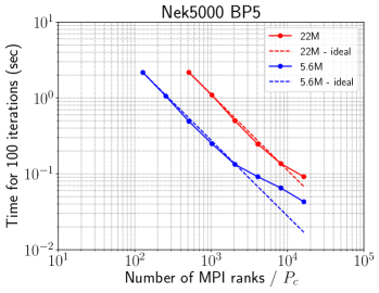
(a) BP5: time vs. $P_{c}$

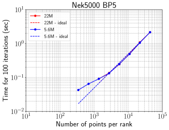
(b) BP5: time vs. $n/P_{c}$

Figure 1: Strong-scale study for BP5-Nek5000 with $n$= 22M and 5.6M. $n/P_{c}$ is the problem size per core, and strong-scale limit is observed at $n/P_{c}=2744$.

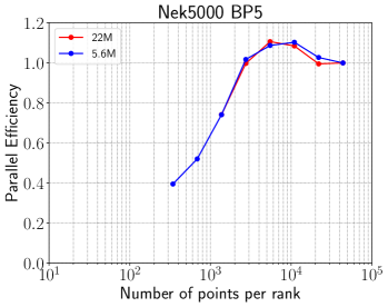
(a) BP5: efficiency vs. $n/P_{c}$

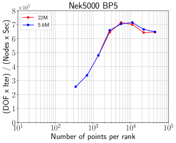
(b) BP5: DOFs vs. $n/P_{c}$

Figure 2: Strong-scale study for BP5-Nek5000. $n/P_{c}$ is the problem size per core. Order unity parallel efficiency can be achieved for $n/P_{c}\geq 2744$.

As an example, we show in Figures 1 and 2 strong-scale performance of Nek5000 using 32 MPI ranks per node on Cetus, the development-level IBM BG/Q at ALCF. The model problem is a 3D Poisson equation solved at different spectral element resolutions, which are described in Section 3 as bake-off problem number 5 (BP5). With polynomial order $p=7$ and number of elements $E=2^{14}$ and $E=2^{16}$, the number of points are $n=$5,619,712 and 22,478,848, respectively. Note that we define the number of points by $n=p^{3}E$ throughout the paper, without redundancy and without boundary condition effects. In other words, $n$ is the total number of parallel unique degrees of freedom, including all boundary unknowns. The polynomial order $p$ is fixed for each direction in the reference element ${\hat{\Omega}}=[-1,1]^{3}$.

Figure 1(a) shows the time versus the number of MPI ranks, $P_{c}$, for each case of fixed $n=22M$ and $n=5.6M$, along with ideal linear scaling plots scaling as $P_{c}^{-1}$. The lower curve, corresponding to the smaller problem, exhibits linear scaling out to $P_{c}=2048$, beyond which the time decreases more slowly. In contrast, scaling for the larger problem is linear out to $P_{c}=8192$ before the performance drop-off is observed. In isolation, one might conclude that the $n=22,478,848$ performance is indicative of good strong-scale behavior. By contrast, the $n=5,619,712$ graph might be viewed with skepticism regarding the ability of the code to strong-scale beyond $P_{c}=2048$.

In fact, if we change the $x$-axis in Figure 1(a) to be $n/P_{c}$, we see that the large and small problem results collapse to a single curve, as evident in Figure 1(b). In this case, for $n/P_{c}\geq 2744$ the solution time is directly proportional to the amount of work on each rank, namely,

$$t_{\mbox{\footnotesize{wall}}}\sim n/(S\,P_{c}),$$ (1)

where $S$ is a constant that scales as the rate of work per rank in this work-saturated limit. From this result, we can infer that we have order unity parallel efficiency for $n/P_{c}\geq 2744$, meaning that for any case with $n/P_{c}>2744$ one can effectively increase the number of processors with a corresponding decrease in time to solution, all at fixed energy and cost, assuming that the machine has enough processors to do so. This is the important promise of distributed-memory parallel computing. We often refer to such a break point (e.g., $n/P_{c}=2744$ in Figure 1(b)) as the strong-scale limit towards which users will naturally gravitate. Running with $n/P_{c}$ significantly exceeding this limiting value implies unnecessarily long runtimes. In practice, users might choose a value of $n/P_{c}$ below this break point if they are willing to tolerate a certain level of inefficiency.

To this end, we define parallel efficiency,

$$\eta(P) := \frac{T_{P_{\min}}\times P_{\min}}{T_{P}\times P},$$ (2)

where $P_{\min}$ is the minimum number of processors used in the strong-scale study (usually, the memory-saturation-bound limit) and $T_{P}$ is the wall-clock time for $P$ processors. (Here, processors means cores, nodes, GPUs, etc., according to the sensible metric for the given platform.) Figure 2(a) shows the corresponding efficiencies for the pair of strong-scale studies from Figure 1. We see that $\eta\approx 0.8$ for $n/P_{c}=1372$ and $\eta\approx 0.5$ for $n/P_{c}=686$. Here, we denote $n_{0.8}=1372$ and $n_{0.5}=686$ as the values of $n/P_{c}$ that correspond to 80% and 50% efficiency, respectively.

We note that in leadership-class computing environments the granularity of the simulation, $n/P$, is a runtime parameter selectable by the user unless $P$ is bounded by the total number of processors accessible in the system. To minimize solution time, users are generally interested in operating as far to the left as possible in Figure 2(a) while staying within a tolerable parallel efficiency, $\eta$. Beyond the strong-scale limit $n/P_{c}=2744$ discussed previously, one could have a 1.6$\times$ speedup by doubling the number of processors (which might be reasonable for long simulations) or a 2$\times$ speedup by quadrupling the number of processors (which likely is not acceptable to most users).

For cross-code comparisons, one must be able to compare rates of work between differing implementations. Here, we retain the independent variable, $n/P$, but change the dependent variable to be

$$\frac{\mbox{\em work}}{\mbox{\em resources}}=\frac{\mbox{\em iterations $\times$ DOFs}}{\mbox{\em nodes $\times$ seconds}}\;=:\;\mbox{DOFs},$$ (3)

where iterations is the number of conjugate gradient (CG) iterations (see the BP definitions in Section 3); DOFs is the number of degrees of freedom (here, grid points); nodes is the number of BG/Q nodes; and seconds refers to the amount of wall-clock time required to perform the given number of CG iterations. (For the bake-off comparisons, the independent variable, $n/P$, is taken to be the number of points per BG/Q node.)

With this background, we have developed a sequence of bake-off problems to generate performance figures similar to Figure 2(b) for a variety of polynomial orders, element counts, operators, and codes (over 2,000 simulations in total). The principal objective is to identify the fastest implementations for each operator, at the given resolution (e.g., polynomial order $p$). Equally important, however, is to identify the peak performance value and the strong-scale limit where performance efficiency drops to a fraction $\eta=0.8$ of this peak value. For the bake-off problems, the number of MPI ranks is fixed to be a large value (generally, $P=512$ nodes, for a total of 16,384 ranks with -c32 mode on BG/Q, using 2 MPI processes per core and 16 cores per node); and the independent variable is the number of degrees of freedom per node, $n/P=(p^{3}E)/P$.

3 Bake-Off Specifications

Table 1: Bake-Off Kernel/Problem Summary

	System		Form	BCs	Quadrature Points	Nodal Points
BK1/BP1	$B{\underline{u}}$	$={\underline{r}}$	scalar	homogeneous Neumann	($p+2$) GL	($p+1$) GLL
BK2/BP2	$B{\underline{u}}_{i}$	$={\underline{r}}_{i}$	vector	homogeneous Neumann	($p+2$) GL	($p+1$) GLL
BK3/BP3	$A{\underline{u}}$	$={\underline{r}}$	scalar	homogeneous Dirichlet	($p+2$) GL	($p+1$) GLL
BK4/BP4	$A{\underline{u}}_{i}$	$={\underline{r}}_{i}$	vector	homogeneous Dirichlet	($p+2$) GL	($p+1$) GLL
BK5/BP5	$A{\underline{u}}$	$={\underline{r}}$	scalar	homogeneous Dirichlet	($p+1$) GLL	($p+1$) GLL
BK6/BP6	$A{\underline{u}}_{i}$	$={\underline{r}}_{i}$	vector	homogeneous Dirichlet	($p+1$) GLL	($p+1$) GLL

The first suite of problems is focused on runtime performance, measured in DOFs for bake-off kernels (BKs) and bake-off problems (BPs). The BKs are defined as the application of a local (unassembled) finite-element operator to a scalar or vector field, without the communication overhead associated with assembly. These tests essentially demonstrate the vectorization performance of the PDE operator evaluation (i.e., matrix-free matrix-vector products, or matvecs). As they represent the most computationally-intensive operations in bake-off problems, the BKs provide an upper bound on realizable floating-point performance (DOFs or MFLOPS) for an application based on such implementations. The BPs are mock-up solvers that use the BKs inside a diagonally preconditioned conjugate gradient (PCG) iteration. The point of testing the BKs inside PCG is to establish realistic memory-access patterns, to account for communication overhead of assembly (i.e., nearest-neighbor exchange), and to include some form of global communication (i.e., dot products) as a simple surrogate for global coarse-grid solves that are requisite for large-scale linear system solves.

To meet these goals in a measurable way, we decided to run the initial BPs on 16,384 MPI ranks (i.e., 512 nodes in -c32 mode) of the IBM BG/Q Cetus at the ALCF, which, by virtue of its convex network partitions and provision for a 17th “OS” core on each node, realizes timings that are repeatable to 3 digits from one job submission to the next. The number of MPI ranks was deemed large enough to reveal obvious strong-scale deficiencies yet small enough to allow minimal queue times for all the cases that needed to be submitted. The range of problem sizes was chosen to span from the performance-saturated limit (a lot of work per node) to beyond the strong-scale limit (very little work per node).

To date, there are six BKs and six BPs. Kernels BK1, BK3, and BK5 operate on scalar fields, while BK2, BK4, and BK6 are corresponding operators applied to vector fields having three components each. Each BP$j$, $j=1,\dots,6$ corresponds to PCG applied to the assembled BK$j$ system, using a matrix-free implementation if that is faster. The even-numbered (vector-oriented) kernels allow amortization of matrix-component memory references across multiple operands and provide a realistic optimization for vector-based applications such as fluid dynamics (three fields) and electromagnetics (six fields). The vector-based implementations can also benefit from coalesced messaging, thus reducing the overhead of message latency, which is important when running in the strong-scale (fast) limit.

The BPs include solution of the mass matrix, $B{\underline{u}}={\underline{r}}$ (BP1–BP2), and the stiffness matrix, $A{\underline{u}}={\underline{r}}$ (BP3–BP6). Approximation orders are $p=1,\dots,15$. For each problem, $q$-point quadrature is used in each direction within the reference element (for a total of $q^{3}E$ quadrature points throughout the domain). For BK1–BK4, Gauss-Legendre (GL) quadrature is used with $q=p+2$. For BK5–BK6, Gauss-Lobatto-Legendre (GLL) quadrature is used with $q=p+1$ quadrature points corresponding to the nodal points of the underlying Lagrangian bases. The nodal and quadrature point choices as well as the boundary conditions (BCs) are summarized in Table 1. The number of elements is $E=2^{k}$, for $k=14,\ldots,21$ ($2^{14}=16,384$ and $2^{21}=2,097,152$) so that at least one element per MPI rank is ensured. The elements are arranged in a tensor-product array with the number of elements in each direction differing by at most a factor of 2. Since the tests are designed to mimic real-world applications, the benchmark codes assume that the elements are full curvilinear elements, approximated by the same order of polynomial, $p$, with iso-parametric mappings and are not allowed to exploit the global tensor-product structure of the element layout. We also note that the geometric matrices are all precomputed in the codes.

4 Mathematical Formulation

We can cast the BP specifications in the context of the following scalar Helmholtz equation,

$$-\;\nabla\cdot\mu\nabla u\;+\;\beta\,u\;=f\;\;\mbox{in $\Omega$},$$ (4)

where $\beta$ and $\mu$ may be nonnegative functions of ${\bf x}\in\Omega$. With $X^{p}$ a finite-dimensional subset of ${\cal H}^{1}$, the Sobolev space comprising square-integrable functions on $\Omega$ whose gradient is also square integrable, the discrete variational formulation of (4) is Find $u\in X^{p}$ such that

$$a(v,u)\;+\;(v,u)_{\beta} = (v,f)\;\;\forall\;v\,\in\,X^{p},$$ (5)

where, for sufficiently regular $v$, $u$, and $f$, we have

$$a(v,u) = \int_{\Omega}\,\mu\nabla v\,\cdot\,\nabla u\,d{\bf x},$$ (6)

$$(v,u)_{\beta} = \int_{\Omega}\,v\,\beta\,u\,d{\bf x},$$ (7)

$$(v,f) = \int_{\Omega}\,v\,f\,d{\bf x}.$$ (8)

We approximate the scalar functions $u$ and $v$ by finite expansion of nodal (Lagrangian) basis functions

$$u({\bf x}) = \sum_{l=1}^{n}u_{l}\,\phi_{l}({\bf x}),$$ (9)

$$v({\bf x}) = \sum_{\hat{l}=1}^{n}v_{\hat{l}}\,\phi_{\hat{l}}({\bf x}).$$ (10)

Insertion of (9)–(10) into (6)–(8) leads to the inner products defined as

$$a(v,u) = {\underline{v}}^{T}A{\underline{u}},$$ (11)

$$(v,u)_{\beta} = {\underline{v}}^{T}B{\underline{u}},$$ (12)

$$(v,f) = {\underline{v}}^{T}{\underline{b}}.$$ (13)

Here, we have introduced the stiffness matrix, $A$, the (weighted) mass matrix, $B$, and the right-hand side, ${\underline{b}}$,

$$A_{\hat{l}l} = a(\phi_{\hat{l}},\phi_{l}),$$ (14)

$$B_{\hat{l}l} = (\phi_{\hat{l}},\phi_{l})_{\beta},$$ (15)

$$b_{\hat{l}} = (\phi_{\hat{l}},f),$$ (16)

where the index sets are $l,{\hat{l}}\;\in\;\{1,\dots,n\}$. The system to be solved is thus

$$H{\underline{u}}={\underline{b}},\quad\mbox{where}\quad H:=\,A\,+\,B.$$ (17)

BPs 1–2 correspond to $\mu=0$ ($A=0$). BPs 3–6 correspond to $\beta=0$ ($B=0$).

The system (17) denotes a generic Galerkin discretization of (5). The point of departure for the finite element/spectral element formulation is in the choice of basis functions, $\phi_{i}$, and choice of quadrature rules for the inner products (6)–(8). With the preceding definitions, we now consider the fast tensor-product evaluations of the inner products introduced in (11)–(12). To begin, we assume $\Omega=\cup_{e=1}^{E}\Omega^{e}$, where the non-overlapping subdomains (elements) $\Omega^{e}$ are images of the reference domain, ${\hat{\Omega}}=[-1,1]^{3}$, given by

$$\left.{\bf x}\right|_{\Omega^{e}}\!\! = \!\!{\bf x}^{e}(r,s,t)$$ (18)

$$= \!\!\sum_{k=0}^{p}\sum_{j=0}^{p}\sum_{i=0}^{p}{\bf x}^{e}_{ijk}\,h_{i}(r)\,h_{j}(s)\,h_{k}(t).\;\;\;$$

Here, the $h_{i}$s are assumed to be the Lagrange interpolation polynomials based on the Gauss-Lobatto-Legendre (GLL) quadrature points, $\xi_{j}\in[-1,1]$, $j=0,\dots,p$. This choice of points yields well-conditioned operators and affords the option of direct GLL quadrature, if desired.

All functions are assumed to have expansions similar to (18). For example, the solution $u({\bf x})$ on $\Omega^{e}$ takes the form

$$\left.u\right|_{\Omega^{e}}=\sum_{k=0}^{p}\sum_{j=0}^{p}\sum_{i=0}^{p}u^{e}_{ijk}\,h_{i}(r)\,h_{j}(s)\,h_{k}(t),$$ (19)

for the $(p+1)^{3}$ unknown basis coefficients in $\Omega^{e}$.

To ensure interelement continuity ($u,v\in X^{p}\subset{\cal H}^{1}$), one must constrain coefficients at shared element interfaces to be equal. That is, for any given sets of index coefficients $(i,j,k,e)$ and $({\hat{\imath}},{\hat{\jmath}},{\hat{k}},{\hat{e}})$,

$${\bf x}_{ijk}^{e}\,=\,{\bf x}_{{\hat{\imath}}{\hat{\jmath}}{\hat{k}}}^{{\hat{e}}} \longrightarrow u_{ijk}^{e}\,=\,u_{{\hat{\imath}}{\hat{\jmath}}{\hat{k}}}^{{\hat{e}}}.$$ (20)

The statement (20) leads to the standard finite element processes of matrix assembly and assembly of the load and residual vectors. Fast matrix-free algorithms that use iterative solvers require assembly only of vectors, since the matrices are never formed. To implement the constraint (20), we introduce a global-to-local map, formally expressed as a sparse matrix-vector product, ${\underline{u}}_{L}=Q{\underline{u}}$, which takes (uniquely defined) degrees of freedom $u_{l}$ from the index set $l\in\{1,\dots,n\}$ to their (potentially multiply defined) local counterparts $u_{ijk}^{e}$. We further define $A_{L}=$block-diag$(A^{e})$, and arrive at the assembled stiffness matrix

$$A=Q^{T}A_{L}Q.$$ (21)

We refer to $A_{L}$ as the unassembled stiffness matrix and its constituents $A^{e}$ as local stiffness matrices. With this factored form, a matrix-vector product can be evaluated as ${\underline{w}}=Q^{T}A_{L}Q{\underline{u}}$, which allows parallel evaluation of the work-intensive step of applying $A^{e}$ to basis coefficients in each element $\Omega^{e}$. Application of the Boolean matrices $Q$ and $Q^{T}$ represents the communication-intensive phases of the process.

5 Matrix-Free $Q_{p}$ Formulations

Efficient matrix-free formulations of $Q_{p}$ tensor-product spaces date back to Fourier-based spectral methods pioneered by Orszag and others in the early 1970s. In a landmark paper, Orszag (1980) showed that the principal advantage of Fourier spectral methods in ${{\rm l}\kern-1.49994pt{\rm R}}^{3}$ derives from the tensor product forms (e.g., (19)), which reduce the cost of applying differential operators for $p^{3}$ degrees of freedom from $O(p^{6})$ to $O(p^{4})$. Orszag further noted that if one exploits symmetries in the one-dimensional operators, the constant can potentially be improved; and, with enough symmetry, such as in the Fourier and Chebyshev cases, the asymptotic complexity can be reduced to $O(p^{3}\log p)$. With the introduction of the spectral element method (SEM), Patera (1984) extended Orszag’s work to a variational framework using Chebyshev bases, and Rønquist and Patera (1987) developed the nodal-bases approach using Gauss-Lobatto-Legendre quadrature that is now commonplace in the SEM and other high-order $Q_{p}$ implementations.

With the use of iterative solvers, the bake-off problems amount to implementing fast matrix-vector products. As noted earlier, matrix-free evaluations are effected with a communication phase for assembly and a local work-intensive phase to evaluate the physics. For the stiffness matrix, $A$, the local matrix vector products ${\underline{w}}^{e}:=A^{e}{\underline{u}}^{e}$ can be implemented in the matrix-free form outlined in 4.4.7 of Deville et al. (2002),

$${\underline{w}}^{e}=\left(\!\!\begin{array}[]{c}D_{1}\\[1.29167pt] D_{2}\\[1.29167pt] D_{3}\end{array}\!\!\right)^{\!\!\!\!\!T}\!\!\!\left(\!\begin{array}[]{ccc}G^{e}_{11}&G^{e}_{12}&G^{e}_{13}\\[1.29167pt] G^{e}_{21}&G^{e}_{22}&G^{e}_{23}\\[1.29167pt] G^{e}_{31}&G^{e}_{32}&G^{e}_{33}\end{array}\!\right)\!\!\!\!\left(\!\!\begin{array}[]{c}D_{1}\\[1.29167pt] D_{2}\\[1.29167pt] D_{3}\end{array}\!\!\right){\underline{u}}^{e}.$$ (31)

Here, the derivative matrices $D_{j}$ involve tensor products of the one-dimensional $(q\times p_{1})$ interpolation (${\hat{J}}$) and derivative (${\hat{D}}$) matrices: $D_{1}={\hat{J}}\otimes{\hat{J}}\otimes{\hat{D}}$, $D_{2}={\hat{J}}\otimes{\hat{D}}\otimes{\hat{J}}$, and $D_{3}={\hat{D}}\otimes{\hat{J}}\otimes{\hat{J}}$, where $p_{1}=p+1$ is the number of nodal points in each direction within an element and $q$ is the corresponding number of quadrature points. For BP5 and BP6, we use GLL quadrature on the $q=p_{1}$ nodal points, so ${\hat{J}}$ becomes the $q\times q$ identity matrix, which yields considerable savings in computational cost.

Each of the geometric factors is a diagonal matrix of size $q^{3}\times q^{3}$ (i.e., comprising only $q^{3}$ nontrivial entries). For each quadrature point $(\eta_{i},\eta_{j},\eta_{k})\in{\hat{\Omega}}$,

$$\left[G^{e}_{mm^{\prime}}\right]_{ijk}=\left[\sum_{l=1}^{3}\frac{\partial r_{m}}{\partial x^{e}_{l}}\frac{\partial r_{m^{\prime}}}{\partial x^{e}_{l}}\right]_{ijk}\!\!\!{\cal J}^{e}_{ijk}\rho_{i}\rho_{j}\rho_{k},$$ (32)

where ${\cal J}^{e}_{ijk}$ is the geometric Jacobian evaluated at the quadrature points and the $\rho_{j}$s are the GL quadrature weights for BP3–BP4 and GLL weights for BP5–BP6. ${\bf G}^{e}$ is a symmetric tensor, $G^{e}_{mm^{\prime}}=G^{e}_{m^{\prime}m}$, so only $6q^{3}$ memory references per element are required for (31), in addition to the $p_{1}^{3}$ reads required to load ${\underline{u}}^{e}$. ${\hat{J}}$ and ${\hat{D}}$ require only $q\times p_{1}$ reads, which are amortized over multiple elements and therefore discounted in the analysis.

The majority of the computational effort in (31) is in application of the $D_{j}$s. Thus, it is worthwhile to explore the complexity for these tensor contractions, which are central to fast matrix-free formulations. We consider two of the many possible approaches. First, we need to evaluate for each element $\Omega^{e}$,

$${\underline{u}}^{e}_{r} = D_{1}{\underline{u}}^{e}\;=\;({\hat{J}}\otimes{\hat{J}}\otimes{\hat{D}}){\underline{u}}^{e}$$ (33)

$${\underline{u}}^{e}_{s} = D_{2}{\underline{u}}^{e}\;=\;({\hat{J}}\otimes{\hat{D}}\otimes{\hat{J}}){\underline{u}}^{e}$$ (34)

$${\underline{u}}^{e}_{t} = D_{3}{\underline{u}}^{e}\;=\;({\hat{D}}\otimes{\hat{J}}\otimes{\hat{J}}){\underline{u}}^{e},$$ (35)

each of which is a map from $p_{1}^{3}$ nodes to $q^{3}=\gamma^{3}p_{1}^{3}$ quadrature points, where $\gamma:=q/p_{1}$.

While the differentiation matrices $D_{j}$ are full, with $\gamma^{3}p_{1}^{6}$ nonzeros, they can be applied in factored form as tensor contractions with only $O(p^{3})$ storage and $O(p^{4})$ work. For example, (33) is typically implemented as

$${\underline{u}}^{e}_{r}=({\hat{J}}\otimes{\hat{I}}\otimes{\hat{I}})({\hat{I}}\otimes{\hat{J}}\otimes{\hat{I}})({\hat{I}}\otimes{\hat{I}}\otimes{\hat{D}}){\underline{u}}^{e},$$ (36)

with ${\hat{I}}$ an appropriately sized identity matrix. More explicitly, (36) is evaluated for $i,j,k\,\in\,\{1,\dots,q\}^{3}$ as

$$({\underline{u}}^{e}_{r})_{ijk}=\sum_{{\hat{k}}=0}^{p}{\hat{J}}_{k{\hat{k}}}\left(\sum_{{\hat{\jmath}}=0}^{p}{\hat{J}}_{j{\hat{\jmath}}}\left(\sum_{{\hat{\imath}}=0}^{p}{\hat{D}}_{i{\hat{\imath}}}u_{{\hat{\imath}}{\hat{\jmath}}{\hat{k}}}\right)\right){\underline{u}}^{e},$$ (37)

which has computational complexity

$$\begin{split}\mbox{W}&=2(qp_{1}^{3}+q^{2}p_{1}^{2}+q^{3}p_{1})\\ &=2p_{1}^{4}(\gamma+\gamma^{2}+\gamma^{3})\end{split}$$ (38)

operations. This cost is nominally repeated for (34)–(35), save for the common term $({\hat{I}}\otimes{\hat{I}}\otimes{\hat{J}}){\underline{u}}^{e}$, which does not need to be re-evaluated. We note that $[D_{1}^{T}\,D_{2}^{T}\,D_{3}^{T}]$ can be applied in a similar fashion, so the total work for (31) with this approach is

$$\mbox{W}=4p_{1}^{4}(3\gamma^{3}+3\gamma^{2}+2\gamma)+15\gamma^{3}p_{1}^{3}.$$ (39)

The $O(p^{3})$ term arises from application of the $3\times 3$ $G^{e}_{mm^{\prime}}$ tensor.

An alternative approach to (33)–(35) is to first interpolate $u$ to the quadrature points, ${\tilde{\underline{u}}}^{e}=J{\underline{u}}^{e}=({\hat{J}}\otimes{\hat{J}}\otimes{\hat{J}}){\underline{u}}^{e}$, followed by differentiation

$${\underline{u}}^{e}_{r} = ({\tilde{I}}\otimes{\tilde{I}}\otimes{\tilde{D}}){\tilde{\underline{u}}}^{e}$$ (40)

$${\underline{u}}^{e}_{s} = ({\tilde{I}}\otimes{\tilde{D}}\otimes{\tilde{I}}){\tilde{\underline{u}}}^{e}$$ (41)

$${\underline{u}}^{e}_{t} = ({\tilde{D}}\otimes{\tilde{I}}\otimes{\tilde{I}}){\tilde{\underline{u}}}^{e},$$ (42)

where ${\tilde{I}}$ and ${\tilde{D}}$ are respectively $q\times q$ identity and derivative matrices on the one-dimensional array of quadrature points. This strategy leads to a complexity of $\mbox{W}=2p_{1}^{4}(3\gamma^{4}+\gamma^{3}+\gamma^{2}+\gamma)$ for the gradient and an overall complexity for (31) of

$$\mbox{W}=4p_{1}^{4}(3\gamma^{4}+\gamma^{3}+\gamma^{2}+\gamma)+15\gamma^{3}p_{1}^{3}.$$

For $\gamma=1$, the second approach yields a reduction in work of $\approx$25% over (37). By contrast, for $\gamma=3/2$ (commonly used in evaluating nonlinear advection terms), the second approach incurs roughly a 12% increase in operation count.

The mass matrix has a similar tensor product form. Specifically,

$${\underline{w}}^{e}=B^{e}{\underline{u}}^{e}=J^{T}{\tilde{B}}^{e}J{\underline{u}}^{e},$$ (43)

where ${\tilde{B}}^{e}=\mbox{diag}(\rho_{i}\rho_{j}\rho_{k}{\cal J}^{e}_{ijk})$ is the diagonal mass matrix on the quadrature points and $J={\hat{J}}\otimes{\hat{J}}\otimes{\hat{J}}$ is the interpolation operator that maps the basis functions to the quadrature points. Application of (43) has a complexity of $4p_{1}^{4}(\gamma^{3}+\gamma^{2}+\gamma)$ operations and $p_{1}^{3}(1+\gamma^{3})$ reads from memory. (We remark that the spectral element method uses a diagonal mass matrix on the GLL points, for overall work and memory complexity of only $p_{1}^{3}$ per element for either the forward or inverse mass matrix application.)

While the tensor contractions have complexity of $O(p^{4})$, every other operation is of order $O(p^{3})$ or lower (e.g., $O(p^{2})$ for surface operations). On traditional architectures, the tensor contractions are effectively implemented as dense matrix-matrix products (e.g., Deville et al. (2002)). On highly threaded architectures, such as GPUs, other approaches that better exploit the tensor structure are often more effective because the straightforward BLAS3 implementations do not expose sufficient parallelism and data reuse. We revisit this point in Section 8.

We further note that the operation count for all tensor contractions can be roughly halved by exploiting the symmetry of the GLL and GL point distributions, as noted by Solomonoff (1992) and Kopriva (2009). Such an approach is used in deal.II and in some of our libParanumal results for the Nvidia V100, as detailed in the Appendix. In addition to operation counts, one must recognize that the kernel (BK) performance can be heavily influenced by whether $q$ or $p+1$ match cache-line sizes or vector-lane widths, which are typically 4 or 8 words wide. Moreover, application of the work-intensive operators, $D_{i}$ in (31) and $J$ in (43), is identical for each element (of the same order, $p$) because these operators are applied in the reference domain ${\hat{\Omega}}$. One can therefore vectorize over blocks of elements, rather than just applying the operators to a single element at a time. If the number of elements per rank is a multiple of (say) 4 or 8, one can easily arrange the data to exploit this level of SIMD parallelism, assuming that there are enough elements per MPI rank.

We close this section by noting that, implemented properly, the tensor-product-based matrix-free formulation requires the optimal amount of memory transfers (with respect to the polynomial order) and near-optimal FLOPs for operator evaluation. The importance of these overhead costs is illustrated in Figure 3, which contrasts the matrix-vector product costs with fully assembled matrices (in block compressed sparse row format) with matrix-free approaches.

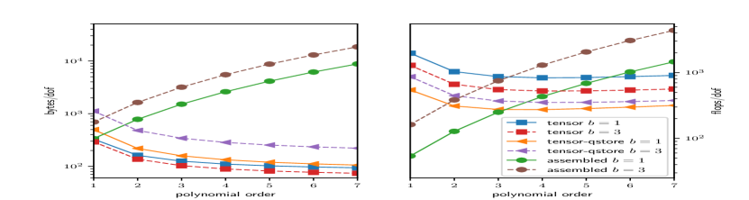
Figure 3: Memory transfer and floating-point operations per degree of freedom for a PDE in 3D with $b$ components and variable coefficients. The “tensor” computes metric terms on the fly and stores a compact representation of the coefficients at quadrature points; the “tensor-qstore” pulls the metric terms into the stored representation as in (32); the “assembled” uses a (block) CSR format.

Table 2: System Configuration

	ALCF BG/Q (Cetus & Mira)	OLCF Summit
Processor	16-core 1.6 GHz IBM PowerPC A2	IBM Power9TM (2/node)
Nodes	2,048 (Cetus), 49,152 (Mira)	4,608
CPU Cores/node	16	42
Total CPU Cores	32,768 (Cetus), 786,432 (Mira)	193,536
Total GPUs	–	27,648 NVIDIA Volta V100s (6/node)
Memory/node	16 GB RAM	512 GB DDR4 + 96 GB HBM2
Peak Performancec	10 PF (Mira)	42 TF
Interconnect	5D Torus Proprietary Network	Mellanox EDR 100F InfiniBand, Non-blocking Fat Tree

6 Bake-Off Performance on BG/Q

In this section, we present results for BP1–6 using Nek5000, MFEM, and deal.II. Nek5000 is an F77 code developed at Argonne National Laboratory and originating from the Nekton 2 spectral element code written at M.I.T. by Rønquist (1988), Fischer (1989), and Ho (1989). MFEM is a general-purpose finite element library written in C++ at Lawrence Livermore National Laboratory with the goal of enabling research and development of scalable finite element discretizations MFEM . The deal.II library of Arndt et al. (2017) is also a C++ code that originally emerged from work at the Numerical Methods Group at Universität Heidelberg, Germany. The main focus of deal.II is the computational solution of partial differential equations using adaptive finite elements. Further algorithmic details for each code are described in the Appendix.

All simulations were performed on the ALCF BG/Q Cetus in -c32 mode. The BG/Q system configuration is shown in Table 2. The initial runs were based on the GNU-based compiler, or briefly gcc. On BG/Q, however, the performance of gcc is much lower than that of the native IBM XL (xlc/xlf) compiler, or briefly xlc, so the battery of tests was rerun by using xlc, save for deal.II, which is unable to link properly with xlc version of Cetus. We present both the gcc and xlc results.

We measured the rate of work in DOFs (3). The principal metrics of interest are

• $r_{\max}$, the peak rate of work per unit resource,

• ${n_{0.8}}$, the local problem size $n/P$ on the node required to realize 80% of $r_{\max}$, and

• $t_{0.8}$, the time per iteration when running at 80% of $r_{\max}$.

Note that ${n_{0.8}}$ is defined in terms of points and that $r_{\max}$ (for any given $p$) is the peak rate of work across all the implementations. The importance of ${n_{0.8}}$, $r_{\max}$, and the scaled ratio, $t_{0.8}=1.25\,\,{n_{0.8}}/r_{\max}$, is discussed in Section 7.

All results are plotted as the rate of work per unit resource (3) versus the number of points per compute node, $n/P$. We used a fixed iteration of 100. To simplify the notation, we will refer to the performance variable—the $y$ axis—as DOFs (or MDOFs, for millions of DOFs). Choosing the number of points per node as the independent variable on the $x$-axis, rather than number of DOFs per node, leads to a data collapse in the case where components of vector fields are computed independently: one obtains a single curve for any number of independent components. When the component systems are solved simultaneously, as in BP2, BP4, and BP6, benefits such as increased data reuse or amortized messaging overhead should manifest as shifts up and to the left in the performance curves. We note that for the scalar problems (BP1, BP3, and BP5), the number of DOFs is equal to the number of grid points.

Figures 4–11 present the BP results using the gcc and xlc compilers for Nek5000, MFEM, and deal.II. In each figure, each line represents a different polynomial order. In all cases, performance is strongly tied to the number of gridpoints per node, $n/P$. In the case of the gcc compilers, Nek5000 and MFEM generally exhibit a performance plateau as $n/P$ increases, whereas deal.II shows a distinct peak.

In the discussion that follows, we focus primarily on the saturated (i.e., peak observable) performance toward the right side of the graphs. On the left side, performance levels drop off to uninteresting values that users would generally never experience. This low-performance regime corresponds to relatively few points per node and is easily avoided on distributed-memory platforms by using fewer processors. While the definition is not precise, the point of rapid performance roll-off represents the strong-scale limit to which most users will gravitate in order to reduce time per iteration. Operating to the right of this point would incur longer run times. This transition point is thus the most significant part of the graph, and its identification is an important part of the BP exercise. A convenient demarcation is ${n_{0.8}}$, which indicates the number of points per node where the performance is 80% of the realizable peak for the given polynomial order $p$. (We reiterate that the peak is taken to be the peak across all codes in the test suite, for each BP.)

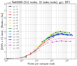
(a) Nek5000 gcc

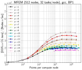
(b) MFEM gcc

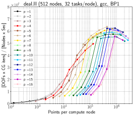
(c) deal.II gcc

Figure 4: BP1 results with gcc compiler using 16,384 MPI ranks on 512 nodes of BG/Q; varying polynomial order ($p=1,...,16$) and quadrature points ($q=p+2$).

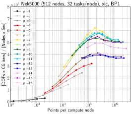
(a) Nek5000 xlc

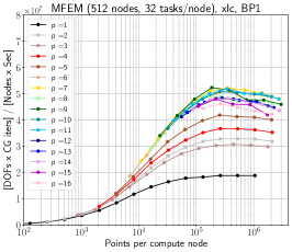
(b) MFEM xlc

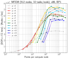
(c) MFEM xlc/x86

Figure 5: BP1 results with xlc compiler using 16,384 MPI ranks on 512 nodes of BG/Q; varying polynomial order ($p=1,...,16$) and quadrature points ($q=p+2$).

6.1 BP1

Figures 4–5 present the BP results for the mass matrix problem, BP1. Figure 4 uses the gcc compilers, while Figure 5 is based on xlc for Nek5000 and MFEM. Nek5000+gcc sustains 27–33 million degrees of freedom per second (MDOFs or mega-DOFs) for polynomial orders $p>4$, save for $p=14$ and 15, which saturate around 25 MDOFs. For MFEM+gcc, a peak performance of 42 MDOFs is realized for $p=3$, which corresponds to $4\times 4\times 4$ bricks for each element. MFEM realizes $>$ 32 MDOFs for $p=2$–4 and $\approx 20$ MDOFs for the majority of the higher-order cases. With gcc, deal.II delivers an impressive 54–64 MDOFs for $p>4$. The highest values are attained for $n/P>450,000$. The ${n_{0.8}}$ for deal.II is also high, however. For example, for $n/P=100,000$, performance is below 30 MDOFs for all $p>9$. The rapid fall-off is related to the way deal.II distributes elements to MPI ranks. The partitioner insists on having at least 8 elements per rank, rather than insisting on a balanced load. Having 8 elements per rank guarantees that 8-wide vector instructions can be issued for any polynomial order but inhibits strong scaling.

Figure 5 again shows the BP1 results but now using the xlc compiler for Nek5000 and MFEM. In addition to the xlc compiler, the Nek5000 results are using intrinsic-directed matrix-matrix product routines for tensor contractions when the inner-product loop lengths are multiples of 4. Separate timings (not shown) indicate that most of the performance gains derive from the xlc compiler, with an additional 5 to 30% coming from the intrinsics, depending on $p$. We see the advantage of xlc and the intrinsics, which boost the peak for Nek5000 to 59 MDOFs for $p=7$ at $n/P=180,000$ and for MFEM to 54 MDOFs at $n=190,000$ for $p=9$. An interesting observation is that with xlc, $p=3$ is the lowest performer (30 MDOFs) for MFEM (ignoring $p=1$), whereas it was the highest (43 MDOFs) with gcc.

Inspired by the deal.II results on x86, the MFEM team also investigated the use of xlc/x86 intrinsics, which allow vectoriziation over blocks of elements. Panel (c) of Figure 5, denoted as MFEM xlc/x86, shows the dramatic improvement resulting from this change. For $p=6$, 7, and 10, MFEM xlc/x86 peaks at around 75 MDOFs, and all polynomial orders except $p=2$ peak at over 50 MDOFs.

6.2 BP3

Figures 6–7 present the BP results for the stiffness-matrix problem, $A{\underline{u}}={\underline{r}}$, with integration based on $q=p+2$ GL points in each direction for each element. The results are similar to those with BP1. With gcc, Nek5000 realizes 20 MDOFs for $p>5$; MFEM achieves a peak of 18 MDOFs for $p=3$, and deal.II reaches a peak of 28 MDOFs. With xlc, Nek5000 reaches a peak of 30–35 MDOFs for $p=6$–8 and 10, and MFEM reaches 20–22 MDOFs for $p=7$–10. The Nek5000 peak for $p=6$ corresponds to $q=8$ quadrature points, for which the intrinsic, BLAS3-based tensor contractions are highly optimized. For MFEM, the largest gains once again derive from the switch to using intrinsics, which lift the MFEM xlc/x86 peak to around 30 MDOFs for $p=6$, 7, and 10.

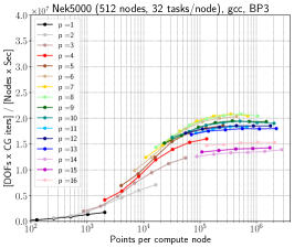
(a) Nek5000 gcc

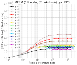
(b) MFEM gcc

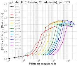
(c) deal.II gcc

Figure 6: BP3 results with gcc compiler on 16,384 MPI ranks on 512 nodes of BG/Q; varying polynomial order ($p=1,...,16$) and quadrature points ($q=p+2$).

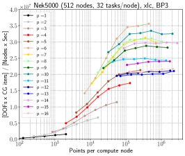
(a) Nek5000 xlc

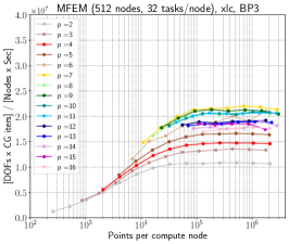
(b) MFEM xlc

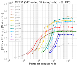
(c) MFEM xlc/x86

Figure 7: BP3 results with xlc compiler on 16,384 MPI ranks on 512 nodes of BG/Q; varying polynomial order ($p=1,...,16$) and quadrature points ($q=p+2$).

6.3 BP5

BP5 (Figures 8–9) solves a Poisson problem using the standard spectral element stiffness matrix in which quadrature is based on the $q=p_{1}$ GLL points, which obviates the need for interpolation, resulting in a shift from (33) to the simpler form (40). The net result is a nearly twofold increase in MDOFs across all cases. Respectively for Nek5000, MFEM, and deal.II, BP5-gcc realizes peaks of 32, 30, and 60 MDOFs, in contrast to 18, 18, and 28 MDOFs for BP3-gcc. For BP5-xlc, the corresponding peaks are 80 and 25 MDOFs for Nek5000 and MFEM. We note that the MFEM xlc/x86 code is not optimized for BP5 because it does a redundant interpolation from mesh nodes to quadrature nodes in this case. The xlc/x86 performance, Figure 9(c), is nonetheless marginally improved over the results of Figure 7(c) because of the slight reduction in the number of quadrature points.

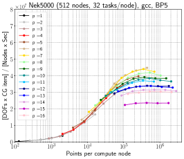
(a) Nek5000 gcc

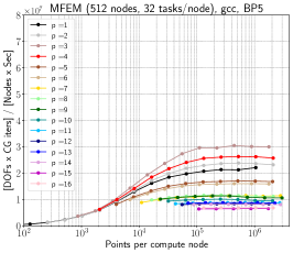
(b) MFEM gcc

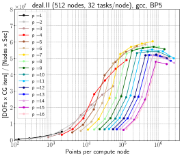
(c) deal.II gcc

Figure 8: BP5 results with gcc compiler on 16,384 MPI ranks on 512 nodes of BG/Q; varying polynomial order ($p=1,...,16$) and quadrature points ($q=p+1$).

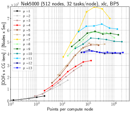
(a) Nek5000 xlc

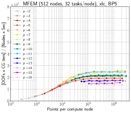
(b) MFEM xlc

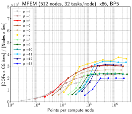
(c) MFEM xlc/x86

Figure 9: BP5 results with xlc compiler on 16,384 MPI ranks on 512 nodes of BG/Q; varying polynomial order ($p=1,...,16$) and quadrature points ($q=p+1$).

6.4 BP2, BP4, and BP6

Results for the vector-oriented BPs are shown in Figure (10) for Nek5000 only. For each of these cases, we solve three systems with three different right-hand sides. The performance results for BP2, 4, and 6 are similar to the corresponding scalar results for BP1, 3, and 5, with the most evident change being that BP6 realizes only 76 MDOFs for $p=7$ instead of the 80 MDOFs attained for BP5.

To better illustrate the potential gain of the vector approach, we plot in Figure 11 the ratio of Nek5000 results in MDOFs for BP2/BP1, BP4/BP3, and BP6/BP5. The gains for very low $n/P$ must be discounted because users will generally not run there, especially for $p=$1, where Nek5000 is not performant. For large $n/P$, the ratios are generally slightly in excess of unity, implying that the Nek5000 multicomponent solver is able to effectively amortize the memory accesses for the geometric components in (32). These ratios trend upwards for smaller $n/P$ values. Near the strong-scale limit, which is in the range $n/P\approx 50,000$–100,000 for Nek5000, we see up to a 1.25-fold increase in MDOFs, which implies that the vector-oriented problems could potentially run with half as many processors with the same efficiency as their scalar counterparts.

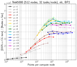
(a) BP2 xlc

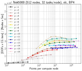
(b) BP4 xlc

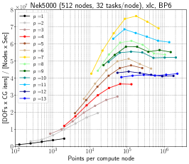
(c) BP6 xlc

Figure 10: Nek5000 results with xlc compiler on 16,384 MPI ranks on 512 nodes of BG/Q with varying polynomial order ($p=1,...,16$).

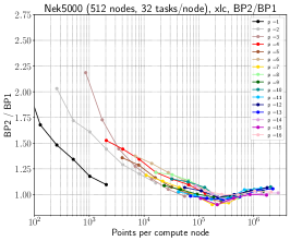
(a) BP2/BP1

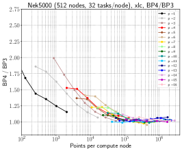
(b) BP4/BP3

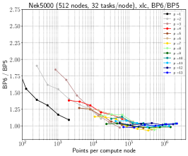
(c) BP6/BP5

Figure 11: Nek5000 results with xlc compiler on the performance ratios of BP2/BP1, BP4/BP3, and BP6/BP5 with varying polynomial order ($p=1,...,16$).

7 CPU Performance Analysis on BG/Q

The results of the preceding sections clearly demonstrate the importance of vector intrinsics in realizing high processing rates. We further remark on some of the cross-code performance variations. One of the optimizations used by deal.II is to exploit the bilateral symmetry of the GL and GLL points in order to cut the number of operations in the tensor contractions by a factor of 2 by using an even-odd decomposition (Solomonoff (1992); Kopriva (2009)). The other, as previously mentioned, organizes the data into 8-element blocks in order to combine favorable vector sizes that help in realizing improved peak performance. Moreover, since the objective of CEED is to develop polyalgorithmic back-ends that will deliver the best performance to the users, our objective is to realize the optimal performance hull over the various implementations. All scaling analysis therefore is based on the best-realized values, not on the values realized by a particular implementation.

7.1 Strong-Scaling Analysis

The broad trends evident in Figures 4–10 also illustrate the importance of the local workload ($n/P$) in realizing peak performance. As noted earlier, for a given problem size $n$, users will generally run on as many processors as possible until the efficiency drops to a tolerable level. This $P$-fold performance multiplier is the most significant factor in realizing large (i.e., thousand-fold or million-fold) speedups in HPC, so understanding inhibitors to increasing $P$ is of paramount importance. For BG/Q, the strong-scale inhibitor for linear systems solves of the type considered here is generally internode latency and not internode bandwidth, as discussed in Fischer et al. (2015) and Raffenetti et al. (2017). We return to this observation shortly.

We see in Figure 9(a) that, for $p=7$, Nek5000 realizes 80 MDOFs for $n/P\approx 175,000$, whereas deal.II achieves a peak 60 MDOFs for $n/P\approx 700,000$. The net result is that for approximately the same work rate (DOFs), whether measured in total energy consumed or node-hours spent, the ability to strong-scale implies that the Nek5000 implementation will run fully 4$\times$ faster because, for a fixed $n$, one can use four times the number of processors. That is, acceptable performance is realized with $n/P=175,000$ rather than the much larger $n/P=700,000$. The point here is not that one code is superior to another. In fact, we do not yet have the xlc data for deal.II and expect that it could be improved substantially. Furthermore, the results show that deal.II’s current mesh partitioning into 8-element blocks clearly inhibits the strong scaling. The point is to stress the importance of achieving reasonable performance at a relatively low value of $n/P$; that is, to be able to strong-scale.

The importance of strong scaling is that it has a direct impact on time to solution when solving problems on large HPC systems. For problems such as considered here, where the work scales linearly with $n$, the time per iteration at 80% efficiency will take the form

$$t_{0.8} = C\frac{{n_{0.8}}}{0.8S},$$ (44)

where $C$ is a problem-dependent constant, $0.8S$ is 80% of the peak realizable speed per node (e.g., the peak MDOFs shown in Figures (4–10)), and ${n_{0.8}}$ is value of $n/P$ where performance matches 80%. The smaller the value of ${n_{0.8}}$, the more processors that can be used and the faster the calculation will run. We stress that reduction of time to solution (at the fast, strong-scale limit) depends critically on minimization of $n_{0.8}/S$ and not solely on increasing the speed of the node, $S$.

7.2 80% Peak vs. Minimum Time

Another way of quantifying minimum time per iteration is to plot parametric curves of DOFs vs. time per iteration, where the independent parameter is $n/P$. Figures 12–13 show a series of such plots for BP1, BP3, and BP5 at order $p=6$ and 13. In addition, we plot the lines corresponding to 80% of peak, which allow identification of the minimum time at which 80% or greater performance is realized.

In the case of $p=6$, the peak for each of the BPs is attained by a different code: MFEM for BP1, Nek5000 for BP3, and deal.II for BP5. The minimum time at $\eta=0.8$ is realized for the same BP/code pairings: 1.2 ms for MFEM–BP1, 1.5 ms for Nek500–BP3, and 1.2 ms for deal.II–BP5. Each time is determined as the intercept of the DOFs time curve with the $0.8\times$DOFs_peak horizontal line in Figure 12. By contrast, for $p=13$, the peak performance is realized by deal.II for all three BPs, whereas the minimum times at $\eta=0.8$ are realized by different codes. For BP1, MFEM-xlc/x86 realizes the minimum time of 5.5 ms; this is the left-most point in Figure 13 that is above the 80% line. For BP3, deal.II has the minimum time-per iteration at 20 ms; none of the other codes are above the 80% mark. For BP5, Nek5000 realizes a minimum time of 2.2 ms at $\eta=0.8$.

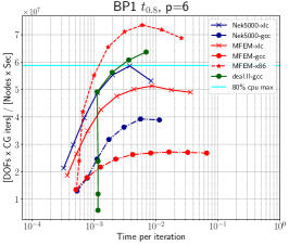
(a) BP1 $t_{0.8}$

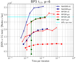
(b) BP3 $t_{0.8}$

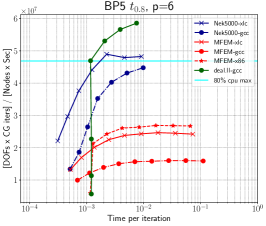
(c) BP5 $t_{0.8}$

Figure 12: DOFs vs time per iteration for BP1, BP3, and BP5 on BG/Q with $p=6$ for Nek5000, MFEM, deall.II.

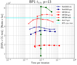
(a) BP1 $t_{0.8}$

(b) BP3 $t_{0.8}$

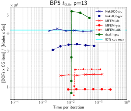
(c) BP5 $t_{0.8}$

Figure 13: DOFs vs time per iteration for BP1, BP3, and BP5 on BG/Q with $p=13$ for Nek5000, MFEM, deall.II.

For both the $p=6$ and 13 cases, we see that the minimum-time graphs for the MFEM-xlc/x86 and deal.II cases exhibit vertical asymptotes as the times are reduced. That is, they cannot deliver smaller times once $n/P$ reaches a critical value. This behavior results from their approach to performance, namely, vectorizing over multiple elements within a single MPI rank. For Nek5000, the minimum times are governed either by communication overhead, as in Figure 12 for $p=6$, or by granularity, as in Figure 13 for $p=13$, where the DOFs vs. time curve is essentially flat. For larger values of $p$ (e.g., $p>13$), the Nek5000 work rates are nearly $p$-independent because there is sufficient work to dominate communication overhead, even at the minimum $n/P$ values where there is only one element per MPI rank.

We have extended the preceding analysis to all polynomial orders $p$ and summarize the results in Figures 14–16. Figure 14 shows the minimum time per iteration that sustains (at least) 80% of peak. The symbol indicates which code realizes this minimum time for the given $p$ (D=deal.II, M=MFEM, N=Nek5000). Where two symbols appear at a given data point, the first indicates the code realizing the minimum time while the second indicates the code that established the peak rate at the given $p$. Figure 15 shows the number of points per node, $n_{0.8}$, associated with each minimum-time point from Figure 14. Figure 16 indicates the corresponding work rate (DOFs) for these points. This value will generally be $r_{0.8}=0.8\times$DOFs_peak unless the performance at the minimum time point exceeds that value. The graphs show results for the odd (scalar) cases as solid lines and for the even (vector) cases as dashed lines.

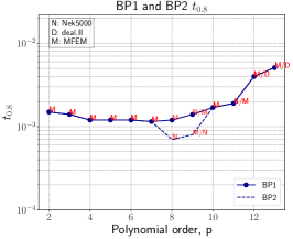
(a) BP1 & BP2 $t_{0.8}$

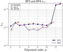
(b) BP3 & BP5 $t_{0.8}$

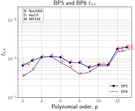
(c) BP5 & BP6 $t_{0.8}$

Figure 14: Minimum time per iteration at 80% of peak, $t_{0.8}$, for BP1, BP3, and BP5 (solid) and BP2, BP4, and BP6 (dashed) vs polynomial order $p$. A/B indicates the associated codes where code A realizes the minimum time and code B realizes the peak performance.

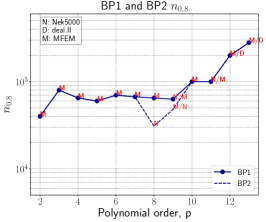
(a) BP1 & BP2 $n_{0.8}$

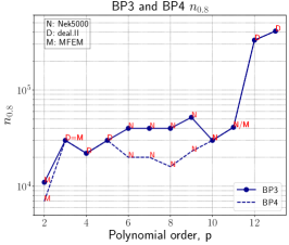
(b) BP3 & BP4 $n_{0.8}$

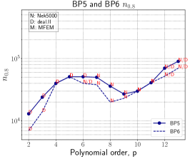
(c) BP5 & BP6 $n_{0.8}$

Figure 15: Points per node, $n_{0.8}$, corresponding to the $t_{0.8}$ values of Figure 14 with the associated the codes.

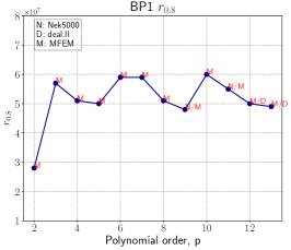
(a) BP1 $r_{0.8}$

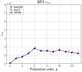
(b) BP3 $r_{0.8}$

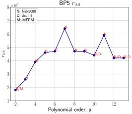
(c) BP5 $r_{0.8}$

Figure 16: Work rate $r_{0.8}=$ [DOFs x CG Iters.] / [Nodes x Sec.] corresponding to the values in Figures 14–15 with the associated codes. (The even BP results are the same as the odd.)

We begin with a discussion of the scalar cases. For polynomial orders $p=1$–11, the minimum time per iteration is in the range 0.6 to 2 ms. The implication of Figure 14 is that, for BG/Q, no simulation will be able to execute PCG iterations at rates faster than 0.5 ms per iteration for BP5 or 1 ms for BP1 and BP3 unless that simulation runs at $\eta<0.8$. Adding more processors does not help reduce the time per iteration. These are the strong-scale bounds, and they are essentially $P$ independent, following the logic that initiates with Figures 1–2.

The range and near-uniformity of these minimal iteration times are not surprising. In the strong-scale limit, communication is on par with local work. Moreover, the size of the local messages is relatively small, $m\leq(p+1)^{2}\ll m_{2}$. Here, $m_{2}$ is the size of a message (in 64-bit words) that costs 2$\alpha$, where $\alpha$ is the latency, or 1/2-round-trip message-passing time for a single 64-bit word. For BG/Q, $\alpha=3.8$ $\mu$s and $m_{2}=845$, as noted by Fischer et al. (2015). At the finest granularity of a single element per processor, there are 26 messages to be exchanged at all polynomial orders, each having a cost between $\alpha$ and 2$\alpha$. On BG/Q, vector reductions are performed in hardware with all-reduce times of approximately $4\alpha$ for all $P$ (Fischer et al. (2015)). Given the two vector reductions required for PCG, we conclude that message-passing costs for a single element per rank on BG/Q lie between $(26+8)\alpha\approx 0.13$ ms and $(52+8)\alpha\approx 0.23$ ms, which is within the range of 20% of of 0.6 ms (the minimum time observed) to 2.0 ms. Larger overheads for the larger times (e.g., 20% of 2.0 ms = 0.4 ms) are likely due to the fact that there are typically more than 26 messages when there is more than one element per rank.

We see in Figure 14 that beyond $p=11$, there is a rise in minimum iteration times with increasing $p$, with the the most rapid rise occurring for BP3, which is the most work-intensive. According to (39)–(5), the leading-order complexity for BK3 is $\approx$ 24–40$p^{4}E$, versus $\approx 12p^{4}E$ for BK1 and BK5. Most of the rise in time per iteration, however, is observed for cases where deal.II performs extremely well and the other codes do not deliver 80% of peak. Consequently, the times rise significantly (by a factor between 4 and 8) because the peak for deal.II is realized only for a minimum of 8 elements per MPI rank.

One of the more significant observations from Figure 14 is that elliptic problems can be solved with polynomial orders up to $p\approx 11$ in the same (or less) time per iteration as their low-order counterparts. (Effective preconditioning is a different topic, studied elsewhere, e.g., Lottes and Fischer (2005); Bello-Maldonado and Fischer (2019), and is slated for a future bake-off study.) In fact, the minimum times for BP5 are realized for $p=9$–11. To understand why, we plot in Figure 15 the number of points per node that corresponds to the time points of Figure 14. Here we can see that the decrease in minimum time for BP5 for $p=7$–9 corresponds to a decrease in the number of points where the minimum time was realized. Fewer points are required to meet the 80% criterion with $p=9$ than with $p=7$, for example. To further test this hypothesis, we plot the corresponding DOFs rates in Figure 16, which is effectively the ratio of the data in Figures 15 and 14. Across the BPs, there is a general upward trend in DOFs as $p$ increases from 2 to 6. In addition, there are distinct peaks where the mod 4 intrinsics apply for Nek5000 (e.g., $p=6$ and 10 for BP3, which correspond to $q=8$ and 12, and $p=7$ and 11 for BP5, for which $q$=8 and 12). The minima in Figure 14 for BP3 and BP5 correspond primarily to locations where smaller problems are running faster, rather than where the processing rates are higher. Overall, we note that the minimum times in the range $p=2$ to 11 correspond to $n_{0.8}\approx$ 30,000–70,000, or 1000–2000 points per rank, in accordance with the 80% efficiency-point observed in Figure 2(a).

The vector results in Figure 14 demonstrate that up to a twofold improvement in minimum time per iteration is realized for several cases. As seen in Figure 15, this reduction comes through a reduction in the minimum problem size that is capable of sustaining 80% of peak through amortized messaging overhead. While some performance gain would be expected through reuse of the geometric factors $G_{mn}$ in (31), that is not the leading source of performance improvement. If it were, it would be manifest in the performance-saturated limit, which is not the case. Note that we elected in Figures 14–15 to base the 80% performance threshold on the scalar peak. The rationale for doing so is that we view the switch to vector solvers as an improvement on a baseline scalar solver and consequently measure performance gains against this scalar baseline.

8 Bake-Off Performance on Summit

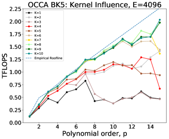
(a) BK5 Tuning

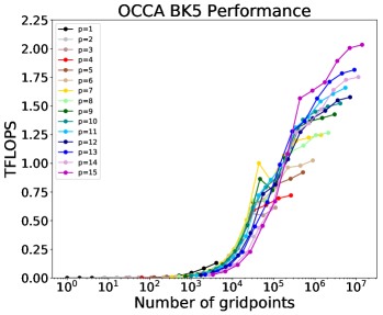
(b) BK5 Tflops

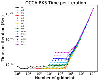
(c) BK5 Timings

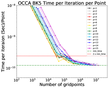
(d) BK5 Timings per point

Figure 17: Single GPU performance: (a) TFLOPS for different kernel tunings. (b) TFLOPS versus problem size $n$ for different polynomial orders, $p$. (c) Execution time versus $n$ for varying $p$. (d) Execution time per point versus number of points, $n$.

With multinode scaling issues addressed through the BP studies, we turn now to node scaling on next-generation accelerator-based architectures. Specifically, we consider the performance of BK5 and BP5 implemented on the Nvidia V100 core on the OLCF Summit using libParanumal, which is an SEM-based high-performance high-order library written in the OCCA kernel language (Medina et al. (2014)). The Summit system configuration can be found in Table 2.

8.1 BK5 on Summit

BK5 amounts to evaluation of the matrix-vector product ${\underline{w}}_{L}=A_{L}{\underline{u}}_{L}$, where $A_{L}$=block-diag($A^{e}$), $e=1,\dots,E$. This kernel is fully parallel because $A_{L}$ represents the unassembled stiffness matrix using the formulation in (31). For performance tuning on the V100, we initially consider only the kernel (BK5), not the full miniapp (BP5), which means we are ignoring communication and device-to-host transfer costs. Our intent is to explore the potential and the limits of GPU-based implementations of the SEM. We seek to determine what is required to get a significant fraction of the V100 peak performance in the context of distributed-memory parallel computing architectures such as OLCF’s Summit.

Figure 17(a) shows the performance for (31) on a single GPU core of Summit through a sequence of OCCA tuning steps, referred to as kernels $K=1,...,10$, for BK5. The number of elements is $E=4096$, and the polynomial order $p$ varies from 1 to 15 ($q=2$ to 16). Each tuned version $K$ is run multiple times, and the time for the kernel is taken by dividing total time by the total number of iterations. This procedure is done to smooth out the noise and to be sure that we are not misguided by the clock resolution limitations.

In the OCCA implementation, each spectral element is assigned to a separate thread block on the GPU with a 2D thread structure. Threads within a block are assigned in a 2D layout with an $i$-$j$ column of the $i$-$j$-$k$ spectral element data assigned to each thread. The individual kernel formulations, $K=1$ to 10, constitute successive improvements in memory management that are described briefly in the Appendix and in detail in Świrydowicz et al. (2019). Kernel 1 sustains 500 GFLOPS for $p=8$–15, while Kernels 9 and 10 reach a peak of 2 TFLOPS for the highest polynomial orders. While the V100 is formally capable of 7 TFLOPS in 64-bit arithmetic, it is well known that memory bandwidth demands constrain the realizable peak to a modest fraction of this value. Figure 17(a) also shows a graph of the empirical roofline as a function of $p$, which is the theoretical maximum performance that can be realized for BK5 based on the number of operations and bytes transferred. We note that the most highly tuned kernels, $K=9$ and 10, attain a significant fraction of the roofline model. The results here and below thus establish upper bounds on performance to be expected in production simulations.

The tuning curves of Figure 17(a) were for $E=4096$, which is the largest case considered. Because GPUs are themselves parallel computers, they have an intrinsic strong-scale limit when the number of points per GPU, ${n_{\mbox{\em\tiny local}}}=n/P$, is insufficient to sustain high work rates. (In this section, we define $P$ to be the number of GPUs, i.e., the number of V100s, used on Summit.) To determine this intrinsic limit, we performed a sequence of BK5 timings using $E=1,\,2,\,4,,\,\dots,\,4096$ for a single GPU, $P=1$. Figure 17(b) shows the V100 TFLOPS for BK5 as a function of ${n_{\mbox{\em\tiny local}}}=p^{3}E$ for $p=1$ to 15. The tight data collapse demonstrates that ${n_{\mbox{\em\tiny local}}}$ is a leading indicator of performance, but the polynomial order is also seen to be important, with $p=15$ realizing a peak of 2 TFLOPS.

Figure 17(c) shows the execution time for the cases of Figure 17(b). Linear dependence is evident at the right side of these graphs, while at the left the execution time approaches a constant for ${n_{\mbox{\em\tiny local}}}<10^{5}$. In the linear regime, the time scales as $O({n_{\mbox{\em\tiny local}}})$, independent of $p$, despite the $O(p{n_{\mbox{\em\tiny local}}})$ scaling of the FLOPs count. This behavior is expected from the roofline analysis—the performance of BK5 is bandwidth limited even for the largest values of $p$ considered. The lower-bound plateaus in Figure 17(c) are readily understood. At the smaller values of ${n_{\mbox{\em\tiny local}}}$, the number of elements is less than 80, which is the number of streaming multiprocessors (SMs, individual compute units) on the V100. Element counts below this value constitute situations in which SMs are idled and the time per iteration is consequently not reduced.

Further insight into the $(p,E,P)$ performance trade-offs can be gained by looking at the execution time per point, shown in Figure 17(d), which also shows the minimal time and the 2$\times$ line, which is twice the minimal execution time per point. For a fixed total problem size, $n$, moving horizontally on this plot corresponds to increasing $P$ and reducing ${n_{\mbox{\em\tiny local}}}$ such that $n={n_{\mbox{\em\tiny local}}}P$. In the absence of communication overhead, one gains a full $P$-fold reduction in the execution if the time per point does not increase when moving to the left. We see in this plot that $p=7$ appears to offer the best potential for high performance, where even at ${n_{\mbox{\em\tiny local}}}=$30,000 the execution time per point is within a small multiple of the minimum realized over all cases. This low value of ${n_{\mbox{\em\tiny local}}}$ is in sharp contrast with the $p=14$ and 15 cases, which cross the $2\times$ line at ${n_{\mbox{\em\tiny local}}}=$200,000. Thus, through additional internode parallelism, the $p=7$ case affords a potential 200/30 $\approx$ 7-fold performance gain over the larger $p$ cases. Of course, this analysis must be tempered by consideration of a full solver that includes communication, particularly for Poisson problems, which require communication-intensive multilevel solvers for algorithmic efficiency. In the next section, we take a step in that direction by analyzing the BP5 performance on Summit.

8.2 BP5 on Summit

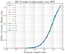
(a) BP5 $p=1,...,10$

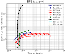
(b) BP5 $p=8$

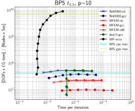
(c) BP5 $p=10$

Figure 18: Multi GPU performance using 24 V100s: (a) BP5 DOFS vs. grid points per node plot for libParanumal (libP) on Summit Summit with $p=1$–10. (b) DOFS vs time per iteration comparison on Summit and BG/Q for $t_{0.8}$ with $p=8$. (c) DOFS vs time per iteration comparison on Summit and BG/Q for $t_{0.8}$ with $p=10$.

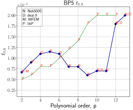
(a) BP5 $t_{0.8}$

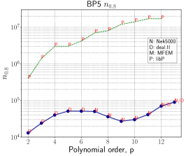
(b) BP5 $n_{0.8}$

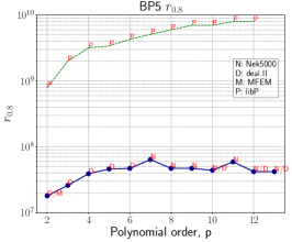
(c) BP5 $r_{0.8}$

Figure 19: BP5 time ($t_{0.8}$), grid points ($n_{0.8}$), and rate ($r_{0.8}$), running from libParanumal (libP) on Summit, and Nek5000, deal.II, and MFEM on BG/Q.

The BP5 implementation on the V100s employs the optimally performing BK5 kernel of the preceding section. All vectors are stored in their local form, following the Nek5000 storage approach described in Appendix A1. The vector operations for PCG, including the diagonal preconditioner, are straightforward streaming operations with a FLOPs count of $n$ or $2n$ and data reads involving only one or two 64-bit words per operation. Assembly for the matrix-vector products (the $QQ^{T}$ operation in (45)) is invoked in two stages. Values corresponding to vertices shared within a GPU are condensed on the GPU. Values for vertices shared between GPUs are sent through the host and then condensed through a pairwise exchange and sum across the corresponding MPI ranks. For all of the studies, we use a total of $P=24$ GPUs: six GPUs on each of four nodes of Summit.

Figure 18(a) shows DOFS vs. $n/P$ curves analogous to Figures 8–9. At 10,000 MDOFs, the peak V100 performance is substantially higher than the peak of 80 MDOFs realized for a single node of BG/Q. The $n_{0.8}$ is also substantially higher on the V100–around 15 million for one node of Summit vs. a maximum of 80,000 for BG/Q. In Figures 18(b) and (c), we plot DOFS vs. time for $p=4$ and 10 for the V100 and for the bake-off codes on BG/Q. We see that, for $p=4$, the minimum time for Summit at 80% of its realized peak is smaller than the $t_{0.8}$ value realized on BG/Q. For $P=10$, Summit can also realize a smaller time per iteration than BG/Q, but not at the realized 80% efficiency value. At that value, the min-time is $0.002$ seconds, which is about three times slower than $t_{0.8}=0.0007$ seconds attained for $p=10$ on BG/Q.

Using plots similar to Figures 18(b) and (c), we generate time ($t_{0.8}$), size ($n_{0.8}$), and DOFs ($r_{0.8}$) curves for libParanumal on Summit and compare these with their BG/Q counterparts in Figure 19. For $p<6$, Summit is able to deliver relatively small values of $t_{0.8}$, subject to the caveat that the $r_{0.8}$ values for Summit in Fig. 19(b) are not fully saturated. For midrange polynomial orders, $p=7$–10, the minimum times on the V100 are roughly a factor of two to three higher than on BG/Q. While the V100 execution rates are higher (Figure 19(c)), they are not sufficiently high to make up for the increased problem size required to sustain 80% of the observed peak. This imbalance results in increased time per iteration, as indicated in (44).

We close this section by noting that the strong-scale time per iteration is not the only performance metric of interest in evaluation of exascale platforms. Cost and energy consumption, which are not assessed in the present studies, are also important concerns in the drive to exascale, and accelerators have been shown to offer advantages with respect to these important metrics.

9 Conclusion

We have presented performance results for highly optimized matrix-free implementations of high-order finite element problems on large-scale parallel platforms and state-of-the-art accelerator nodes. The data are the results of an initial suite of benchmark problems that will be extended in the future to include preconditioning comparisons, nonsymmetric operators, and other geometric configurations. Four teams participated in the study—three running on the BG/Q, Cetus, at ALCF, and one running on the OLCF V100-based platform, Summit.

For BG/Q, no single strategy was best across all the BPs. Vectorization across elements (i.e., in cases with more than one element per MPI rank) could in some cases yield greater than 1.25$\times$ speedup over single-element performance, implying that 80% efficiency could not be realized at the granularity limit of a single element per processor. Reduction in floating-point operation counts can be realized by exploiting the bilateral symmetry of the nodal and quadrature point distributions. Effective time reductions for this approach requires careful local memory management.

For $p<12$, the minimum time per iteration at 80% efficiency is fairly uniform with $t_{0.8}\approx$ 0.6–1.2 ms at $n/P$ values of 30,000–70,000 points per node for the midrange polynomial orders. For BP3 and BP5, the midrange processing rates were substantially higher than the lower order polynomial cases, implying that, in the same time, the higher-order solutions could process more points (i.e., higher resolution) and achieve higher accuracy (higher-order polynomial approximation). In several cases, a twofold reduction in $t_{0.8}$ could be realized by solving block diagonal systems simultaneously in order to amortize communication latency at the strong-scale limit, as demonstrated in the comparison of BP2, BP4, and BP6 with their scalar counterparts.

On Summit, we found that highly tuned OCCA kernels could deliver 2 TFLOPS, which is a significant fraction of the peak 7 TFLOPS cited for a single V100 GPU. Moreover, the OCCA performance is near the bounds established by bandwidth-limited roofline performance model for BK5 (and, for other kernels, as shown by Świrydowicz et al. (2019)). For BP5, Summit realizes in excess of 10,000 MDOFs per node, a factor of 125 larger than a single node of Cetus. The $n_{0.8}$ values, however, are also much larger– approximately $10^{7}$ vs. $10^{5}$ on Cetus. Consequently, $t_{0.8}$ values are superior to the values realized on Cetus for $p<6$, but are larger for $p=7$–11, with Summit times 2 to 3 times larger than $t_{0.8}$ found on Cetus. For $p>11$ the times are again comparable, but are significantly larger (on both platforms) than those for $p\leq 11$.

Funding

This material is based upon work supported by the U.S. Department of Energy, Office of Science, under Contract DE-AC02-06CH11357. This Work is also performed under the auspices of the U.S. Department of Energy under Contract DE-AC52-07NA27344 (LLNL-JRNL-782135). Kronbichler is supported by the German Research Foundation (DFG) under the project “High-order discontinuous Galerkin for the EXA-scale” (ExaDG) within the priority program “Software for Exascale Computing” (SPPEXA), grant agreement no. KR4661/2-1, and the Bayerisches Kompetenznetzwerk für Technisch-Wissenschaftliches Hoch-und Höchstleistungsrechnen (KONWIHR).

Appendix: Algorithmic Description

Algorithmic approaches and their implementations are discussed for Nek5000, MFEM, deal.II, and libParanumal.

Appendix A1: Nek5000

A key feature of Nek5000 is that all data are stored in local form. That is, for any function in $X^{N}\subset C^{0}$, there exists a local vector ${\underline{u}}_{L}=Q{\underline{u}}$. (In fact, the local form, ${\underline{u}}_{L}$, also exists for discontinuous functions, but the global form, ${\underline{u}}$, does not.) If the function is in $C^{0}$, then shared face and edge values are stored redundantly, which means that computations of inner products, daxpys, and other vector operations are doing roughly a factor of $((p+1)/p)^{3}$ extra work. Moreover, inner products need to be weighted to account for repetition of the redundantly stored values unless they are computed prior to residual assembly. The advantage of the local storage format is that the near-neighbor data exchange can be effected in a single communication phase as follows. First, we note that the matrix-vector product ${\underline{w}}=B{\underline{v}}=Q^{T}B_{L}Q{\underline{v}}$ in local form becomes

$${\underline{w}}_{L}=Q{\underline{w}}=Q(Q^{T}B_{L}Q){\underline{v}}=QQ^{T}\,B_{L}\,{\underline{v}}_{L}.$$ (45)

The $QQ^{T}$ operation, often referred to as direct-stiffness summation (see Patera (1984)), corresponds to an exchange and sum of values between shared vertices and is implemented in the general-purpose communication library gslib, which supports other associative/commutative operations (e.g., min, max, multiplication) for scalar and vector fields (see Fischer et al. (2008)). gslib implements the communication and local operator evaluation for several Boolean matrix types other than the symmetric $QQ^{T}$ form. An advantage of using the form in (45) is that data that is interior to elements or on domain boundaries is never moved. Unlike $Q$ or $Q^{T}$ in isolation, the symmetric form $QQ^{T}$ avoids reshuffling of data between global and local layouts.

For Nek5000, (31) is applied element-by-element, with each local matrix vector product ${\underline{w}}^{e}=A^{e}{\underline{u}}^{e}$ applied in three phases: gradient of $u$, application of ${\bf G}$, followed by gradient-transpose. These operations are detailed in subroutine axe in Algorithm 1. The tensor-product contractions for the gradient and gradient-transpose operations are expressed as BLAS3 matrix-matrix products—though rarely as dgemm, since that routine is typically optimized for much larger values of $p_{1}$ than encountered in FEM/SEM applications. Fast contractions are typically best realized by writing different code for each polynomial order, illustrated for the case $p_{1}=8$ shown in mxm8 in Algorithm 1 and the BG/Q intrinsic version mxm_bgq_8 in Algorithm 2. For application of ${\bf G}$, all six elements of the tensor are stored for unit-stride access, as seen in axe.

Algorithm 1 Nek5000 implementation pseudocode for (31). mxm8 is called for tensor contraction lengths of 8. On BG/Q, mxm8 is replaced by mxm_bgq_8 of Algorithm 2.

 subroutine ax(rho,wL,uL,g,mask,ur,ur,ut,n,nel,gsh)! Compute wL=A*uL and rho = wL’*uL real wL(n*n*n,nel),ul(n*n*n,nel,g(6*n*n*n,nel) real mask(n*n*n*nel),ur(n*n*n),us(n*n*n),ut(n*n*n) integer gsh rho = 0 do e=1,nel   call axe(rho,wL(1,e),uL(1,e),g(1,e),ur,us,ut,n) enddo rho = glsum(rho,1)         ! sum over all P call gs_op(gsh,wL,’+’)     ! wL = QQ^T wL do i=1,n*n*n*nel           ! Restrict Dirichlet    wL(i,1)=mask(i)*wL(i,1) ! boundary values to 0 enddo endc-------------------------------------------------- subroutine axe(rho,w,u,g,ur,us,ut,n) common /derivatives/ D(lnn),Dt(lnn) call loc_grad3  (ur,us,ut,u,n,D,Dt) do i=1,n*n*n   wr = g(1,i)*ur(i) + g(2,i)*us(i) + g(3,i)*ut(i)   ws = g(2,i)*ur(i) + g(4,i)*us(i) + g(5,i)*ut(i)   wt = g(3,i)*ur(i) + g(5,i)*us(i) + g(6,i)*ut(i)   ur(i) = wr   us(i) = ws   ut(i) = wt enddo call loc_grad3t (w,ur,us,ut,n,D,Dt) do i=1,n*n*n    rho = rho + w(i)*u(i) enddo endc------------------------------------------------- subroutine loc_grad3(ur,us,ut,u,n,D,Dt) real ur(n,n,n),us(n,n,n),ut(n,n,n),u(n,n,n) real D(n,n),Dt(n,n) call mxm(D ,n,u,n,ur,n*n) do k=1,n    call mxm(u(1,1,k),n,Dt,n,us(1,1,k),n) enddo call mxm(u,n*n,Dt,n,ut,n) endc------------------------------------------------- subroutine mxm8(a,n1,b,n2,c,n3) real a(n1,8),b(8,n3),c(n1,n3) do j=1,n3 do i=1,n1    c(i,j) = a(i,1)*b(1,j) + a(i,2)*b(2,j)           + a(i,3)*b(3,j) + a(i,4)*b(4,j)           + a(i,5)*b(5,j) + a(i,6)*b(6,j)           + a(i,7)*b(7,j) + a(i,8)*b(8,j) enddo enddo end

Algorithm 2 QPX Intrinsics routine for $C=AB$ with inner-product length 8.

subroutine mxm_bgq_8(a,n1,b,n2,c,n3)real(8)  a(n1,8),b(8,n3),c(n1,n3)vector(real(8)) av1,av2,av3,av4,av5,av6,av7,av8vector(real(8)) bv1,bsv1,bsv2,bsv3,bsv4vector(real(8)) bv2,bsv5,bsv6,bsv7,bsv8,cvcall alignx(32, a(1,1))call alignx(32, b(1,1))call alignx(32, c(1,1))do i = 1, n1, 4  av1 = vec_ld(0,a(i,1))  av2 = vec_ld(0,a(i,2))  av3 = vec_ld(0,a(i,3))  av4 = vec_ld(0,a(i,4))  av5 = vec_ld(0,a(i,5))  av6 = vec_ld(0,a(i,6))  av7 = vec_ld(0,a(i,7))  av8 = vec_ld(0,a(i,8))  do j = 1, n3    bv1  = vec_ld(0,b(1,j))    bv2  = vec_ld(0,b(5,j))    bsv1 = vec_splat(bv1, 0)    bsv2 = vec_splat(bv1, 1)    bsv3 = vec_splat(bv1, 2)    bsv4 = vec_splat(bv1, 3)    bsv5 = vec_splat(bv2, 0)    bsv6 = vec_splat(bv2, 1)    bsv7 = vec_splat(bv2, 2)    bsv8 = vec_splat(bv2, 3)    cv =  vec_mul (av1, bsv1)    cv =  vec_madd(av2, bsv2, cv)    cv =  vec_madd(av3, bsv3, cv)    cv =  vec_madd(av4, bsv4, cv)    cv =  vec_madd(av5, bsv5, cv)    cv =  vec_madd(av6, bsv6, cv)    cv =  vec_madd(av7, bsv7, cv)    cv =  vec_madd(av8, bsv8, cv)    call vec_st(cv, 0, c(i,j))  enddoenddoendend

Appendix A2: MFEM

MFEM supports a set of HPC extensions targeting CPU architectures. This functionality is implemented as template classes that require the specification of parameters such as the solution’s polynomial order, the type of the mesh element (quad, hex, etc.), and the order of the quadrature rule, to be given at compile time. This allows the compiler to optimize the compute-intensive inner loops by using loop unrolling, inlining, and even autovectorization in some cases. In addition to the template approach, the HPC extensions implement better algorithms, taking full advantage of the tensor product structure of the finite element basis on tensor product mesh elements: quads and hexes. Furthermore, the HPC extensions support various levels of operator assembly and evaluation. These levels include full matrix assembly to CSR format, partial assembly (where data at quadrature points is computed and stored during the assembly and later used in the operator evaluation), and an “unassembled” approach where assembly is a no-op and all computations are performed on the fly during the operator evaluation.

A recent addition to MFEM is the introduction of CPU SIMD intrinsics to the HPC extension classes where vectorization is explicitly applied across a fixed number of elements; for example, on CPUs with 256-bit SIMD instructions, four elements are processed simultaneously by using double-precision arithmetic.

In this paper, we present results based on the MFEM HPC extensions both with and without the use of SIMD intrinsics.

Implementation Details.

In MFEM, the subdomain restriction, $P$, can be represented by two classes: (1) ConformingProlongationOperator when the finite element space has no hanging nodes or (2) HypreParMatrix in all other cases. All tests in this paper use the first class since we do not consider AMR meshes. This class allows for an optimized implementation because all nonzero entries of $P$ are equal to $1$.

In the HPC extension of MFEM, the element restriction matrix $G$ is represented by an implicit template class concept that allows flexible optimized implementations. The specific class used in the numerical tests is class H1_FiniteElementSpace, which represents $G$ through an indirection array of integer offsets: every row of $G$ has exactly one nonzero entry that is equal to $1$, and therefore, only its column index has to be stored. The class concept assumes, and H1_FiniteElementSpace implements, two main methods, VectorExtract and VectorAssemble, which implement the action of $G$ and $G^{T}$ for one element or a small batch of elements.

The basis evaluator operator $B$ also is represented in MFEM by a template class concept. In the tests considered here, the specific class template we used is TProductShapeEvaluator instantiated in 3D (hex element) for a fixed number of DOFs and quadrature points in each spatial dimension. The main methods in the class are Calc and CalcT, for the case of a mass matrix operator, and CalcGrad and CalcGradT, for the case of a diffusion operator.

The combined action of $G$ and $B$ for one element, or a small batch of elements, is represented in the template class FieldEvaluator, which defines the methods Eval and Assemble for the action of $BG$ and $G^{T}B^{T}$, respectively.

The discretization operator is represented by the template class concept of a physics“kernel.” The kernel is responsible for defining the specific form of $B$ that is required (e.g., $B$ is a different operator for mass and diffusion) and the specific operations for defining (assembling) and using the quadrature point data, $D$. In the numerical tests, we used the kernel class templates TMassKernel and TDiffusionKernel.

Putting all these components together, MFEM defines the processor-local version of the discretization operator, $A_{L}=G^{T}B^{T}DBG$, as the template class TBilinearForm. The main class methods are Assemble, for partial assembly, and Mult, for operator evaluation.

As an example of the implementation, the method Mult of TBilinearForm can be written roughly (ignoring the template parameters and some of the method parameters) as follows.

void TBilinearForm::Mult(const Vector &x, Vector &y){   y = 0.0;   FieldEvaluator solFEval(...,                           x.GetData(), y.GetData());   const int NE = mesh.GetNE(); // num. elements   for (int el = 0; el < NE; el++)   {      // declare ’R’ with appropriate type      solFEval.Eval(el, R);      kernel_t::MultAssembled(0, D[el], R);      solFEval.Assemble(R);   }}Clearly, a lot of the details are hidden in the calls solFEval.Eval() and solFEval.Assemble(). Note that the compiled method Mult has no function calls because all methods inside its call tree are force inlined by adding the __attribute__((always_inline)) specification to their definition.

Appendix A3: deal.II

The deal.II finite element library (Arndt et al., 2017), written in the C++ programming language, aims to enable rapid development of modern finite element codes. The library provides support for adaptive meshes with hanging nodes, a large number of finite elements, and delivers functions and classes implementing code patterns in typical matrix assembly tasks with backends to PETSc and Trilinos; see Arndt et al. (2017) and references therein. For high-order computations on elements with tensor product shape functions, there is a separate “matrix-free” module (Kronbichler and Kormann, 2012) optimized for cache-based architectures, exemplified in the step-37, step-48, and step-59 tutorial programs of the library.

The matrix-free module lets the user specify operations on quadrature points in several ways. The most generic interfaces are convenience access operations, organized through a class called FEEvaluation, in terms of the values and gradients of the tentative solution and test functions, respectively. The geometric factors are precomputed for a given mesh configuration—which can be deformed through an arbitrary high-order mapping—and get implicitly applied when accessing a field, such as the gradient of the input vector via FEEvaluation::get_gradient(). For the case of the 3D Laplacian, this approach would access 10 data fields for quadrature points, namely, $9=3^{2}$ for the inverse of the Jacobian $(\mathcal{J}^{e})^{-1}$ and one field for the determinant of the Jacobian times the quadrature weight $\rho$. Depending on the operators called at the user level, only the necessary data is loaded from memory. For specialized operators, such as the Laplacian, an alternative entry point is to access gradients and values in the reference coordinates and apply geometry and the operator by an effective tensor $\rho(\mathcal{J}^{e})^{-1}(\mathcal{J}^{e})^{-T}$, which reduces the data access to 6 fields for the symmetric rank-2 tensor. This effective tensor format is used for the BP3–BP6 problems with deal.II.

The global input and output vectors in the matrix-free operator evaluation connect to the tentative solution and test function slot on the element level, respectively. The vectors are natively implemented in deal.II and stored and treated in fully distributed format outside the integration tasks. Their local arrays contain some space beyond the end of the locally owned range in order to support an in-place transformation via MPI_Isend and MPI_Irecv without a deep copy of all vector entries. Furthermore, the extraction of the local vector for the cell operations is done immediately prior to the interpolation operations $B$ and $B^{T}$ to ensure that the data remains in caches of the processor.

The actions of $G$, $B$, $B^{T}$, and $G^{T}$ are provided by the read_dof_values, evaluate, integrate, and distribute_local_to_global functions of the class FEEvaluation. Since the interpolation operations $B$ and $B^{T}$ are arithmetically heavy also when using optimal sum factorization algorithms (Deville et al. (2002)), deal.II uses SIMD instructions on supported architectures with vectorization over several cells (Kronbichler and Kormann, 2012). The SIMD arrays “leaks” into the user code in the form of a tensor of SIMD type called VectorizedArray<double> in FEEvaluation::get_gradient(), with each lane of the SIMD vector returning data to a different cell. However, typical application codes are templated on the return type and become almost transparent of this fact. The C++ template arguments also enable auxiliary operators, such as multigrid V-cycles for preconditioning, to be easily implemented in single precision. The code automatically detects the case when node points and quadrature points coincide, as well as the more general case when one first must interpolate from the nodal values into quadrature points. The arithmetic of local operations is reduced almost half by a so-called even-odd decomposition that speeds up higher-order computations (Solomonoff, 1992; Kopriva, 2009).

Inside the one-dimensional kernels of sum factorization, the deal.II implementation applies a particular optimization to reduce the arithmetic operations by the so-called even-odd decomposition (Solomonoff, 1992; Kopriva, 2009). It relies on the fact that the basis functions and quadrature points are symmetric about the center $0$ of the one-dimensional reference element $(-1,1)$. If we denote the basis functions of degree $p$ by $\varphi_{i}$, $i=1,\ldots,p+1$, and quadrature points by $\xi_{j}$, $j=1,\ldots,q$, the symmetry implies $\varphi_{i}(\xi_{j})=\varphi_{p+2-i}(\xi_{q+1-j})$. For example, the one-dimensional interpolation matrix $S_{ji}=\varphi_{i}(\xi_{j})$ for the case $p=3$ and $q=5$ is of the form

$$S=\begin{pmatrix}s_{1}&s_{2}&s_{3}&s_{4}\\ s_{5}&s_{6}&s_{7}&s_{8}\\ s_{9}&s_{10}&s_{10}&s_{9}\\ s_{8}&s_{7}&s_{6}&s_{5}\\ s_{4}&s_{3}&s_{2}&s_{1}\end{pmatrix},$$ (46)

for some numbers $s_{1},\ldots,s_{10}$, representing only $10$ distinct entries in this $(q)\times(p+1)=5\times 4$ matrix. The interpolation from the $p+1$ nodal values to the $q$ quadrature points (i.e., the matrix-vector product $\underline{v}=S\underline{u}$) is then decomposed in the following three steps:

• Decompose the vector $\underline{u}$ into the even part $\underline{u}^{+}$ and the odd part $\underline{u}^{-}$. For the $5\times 4$ example, this yields

  $$u^{+}_{1}=u_{1}+u_{4},\quad u^{+}_{2}=u_{2}+u_{3},$$

  $$u^{-}_{1}=u_{1}-u_{4},\quad u^{-}_{2}=u_{2}-u_{3}.$$

• Perform the matrix-vector product on the even and odd contributions separately,

  $$\underline{v}^{+}=S^{+}\underline{u}^{+},\quad\underline{v}^{-}=S^{-}\underline{u}^{-},$$

  with the $\left\lceil\frac{q}{2}\right\rceil\times\left\lceil\frac{p+1}{2}\right\rceil$ matrix $S^{+}$ with entries

  $$S^{+}_{ij}=\frac{1}{2}\left(S_{i,j}+S_{i,p+1-i}\right)$$

  and the $\left\lfloor\frac{q}{2}\right\rfloor\times\left\lfloor\frac{p+1}{2}\right\rfloor$ matrix $S^{-}$ with entries

  $$S^{-}_{ij}=\frac{1}{2}\left(S_{i,j}-S_{i,p+1-i}\right).$$

• Form the final vector $\underline{v}$ by concatenating the even and odd parts of $\underline{v}^{+}$ and $\underline{v}^{-}$, respectively. For the $5\times 4$ example, the result is

  $$v_{1}=v^{+}_{1}+v^{-}_{1},\quad v_{2}=v^{+}_{2}+v^{-}_{2},\quad v_{3}=v_{3}^{+},$$

  $$v_{4}=v^{+}_{2}-v^{-}_{2},\quad v_{5}=v^{+}_{1}-v^{-}_{1}.$$

Note that the entries of the matrices $S^{+}$ and $S^{-}$ internally contain an addition and a multiplication, but these contributions are precomputed. As a consequence, the $(p+1)q$ additions and multiplications (fused multiply-accumulates, FMAs) of the naive matrix-vector product are turned into two matrix-vector multiplications of size $\frac{p+1}{2}\times\frac{q}{2}$, thus reducing the number of FMAs to $\frac{(p+1)q}{2}$. Since the number of additions and subtractions $(p+1)+q$ is of lower complexity, the even-odd decomposition approximately halves the operation count for the 1D kernel. Similar techniques are possible for the reference-cell derivatives with symmetry relation $\varphi^{\prime}_{i}(\xi_{j})=-\varphi^{\prime}_{p+2-i}(\xi_{q+1-j})$.

An important ingredient to make the even-odd decomposition competitive is the way the intermediate results $\underline{u}^{\pm}$ and $\underline{v}^{\pm}$ are handled by the implementation. Since the small matrix multiplication kernels are often limited by the load/store (to L1 cache) rather than actual arithmetics, all temporary results should ideally be kept in registers. In deal.II, the loop kernels are written using C++ templates on both $p$ and $q$, giving loop bounds and vector sizes that are compile-time constants. Up to degrees of approximately $p=9$, register allocation policies of compilers such as gcc keep the values $u^{+}_{1},\ldots,u_{5}^{+}$ and $u^{-}_{1},\ldots,u_{5}^{-}$ in 10 registers. With two additional registers for the two sums $v_{j}^{+}$ and $v_{j}^{-}$ that are eventually written into the respective positions $v_{j}$ and $v_{q+1-j}$, and some spare registers to hold some entries of $S^{+}$ and $S^{-}$, no extra load/store operations are necessary for architectures with 16 visible floating-point registers, assuming the nowadays usual out-of-order execution and register renaming capabilities to hide the latency of the two FMAs. As shown by the analysis of Kronbichler and Kormann (2019), performance is slightly lower for $p=1$ on architectures with FMA support, similar for $p=2,3$, but by $1.3\times$ to $1.7\times$ for $p\geq 4$, when compared with optimized dense matrix multiplication kernels for small matrices analogous to what is done in libxsmm (Heinecke et al., 2015).

Appendix A4: libParanumal

The GPU results of Section 8 were based on the libParanumal library, which is an experimental testbed for exploring high-performance kernels that can be integrated into existing FEM/SEM codes as accelerator modules. The kernel code is written in OCCA (Medina et al. (2014)), which can produce performant CUDA, OpenMP, or OpenCL code. All the current cases were run on OLCF Summit’s Nvidia V100s using CUDA.

Here, we briefly describe the libParanumal development for BK5 through the ten successive kernels indicated in Figure 17(a). Each kernel $K$ includes the optimizations in kernel $K-1$ unless otherwise indicated. These kernels are described in detail by Świrydowicz et al. (2019).

• Kernel 1 corresponds to a straightforward implementation of (31). Each spectral element is assigned to a separate thread block on the GPU with a 2D thread structure. Threads within a block are assigned to an $i$-$j$ column in the $i$-$j$-$k$ spectral element data structure. Entries of ${\underline{u}}^{e}$ are fetched from global memory as needed, and the partial sums in the last loop are added directly to the global memory array to store the final result. This kernel achieves 500 GFLOPS, which is one-fifth of the predicted empirical roofline.

• In Kernel 2 all variables except for the final result are declared by using const. The gains are marginal for $p>7$.

• In Kernel 3 all of the $k$ loops are unrolled, leading to significant gains for $p>7$.

• In Kernel 4 the $k$ loop is placed exterior to the $i$ and $j$ thread loops, making $k$ the slowest running index.

• In Kernel 5 an auxiliary shared-memory array is replaced by two smaller ones.

• In Kernel 6 the input vector ${\underline{u}}^{e}$ is fetched into shared memory.

• In Kernel 7 global memory transactions are reduced by caching data at the beginning of the kernel and writing the output variable only once. This optimization improves performance by about 40%.

• In Kernel 8 arrays are padded for the cases $p=7$ and 15 to avoid shared-memory bank conflicts.

• In Kernel 9 ${\underline{u}}^{e}$ is fetched to registers, $p_{1}$ entries at a time.

• In Kernel 10 three two-dimensional shared-memory arrays are used for partial results.

The results for Kernel 10 are aligned with the empirical roofline model and achieve a peak of 2 TFLOPS for $p=15$. Algorithm 3 gives the pseudocode.

Algorithm 3 libParanumal pseudocode for BK5, ${\underline{w}}_{L}=A_{L}{\underline{u}}_{L}$ corresponding to Kernel 10 of 17(a).

1:for $e\,\in\,\{1,2,\dots,E\}$ do

2:    for $i,j,k\,\in\,\{1,2,\dots,p_{1}\}$ do

3:       If $k=0$, load ${\hat{D}}$ to shared memory

4:       Declare register variables $r_{qr}$, $r_{qs}$, $r_{qt}$.

5:    end for

6:    for $i,j,k\,\in\,\{1,2,\dots,p_{1}\}$ do

7:       Load $J$ (Jacobian)

8:       Declare $q_{r}$,$q_{s}$,$q_{t}$:=0.

9:       $q_{r}=\sum_{n}{\hat{D}}_{in}u_{nji}^{e}$

10:       $q_{s}=\sum_{n}{\hat{D}}_{jn}u_{kni}^{e}$

11:       $q_{t}=\sum_{n}{\hat{D}}_{kn}u_{kjn}^{e}$

12:       Set $r_{qr}=q_{r}$, $r_{qs}=q_{s}$, $r_{qt}=q_{t}$.

13:       ${\underline{w}}^{e}_{kji}=\beta J^{e}_{kji}*u^{e}_{kji}$

14:    end for (synchronize threads)

15:    for $i,j,k\,\in\,\{1,2,\dots,p_{1}\}$ do

16:       Load $G_{00},\,G_{01}\,G_{02}$.

17:       $\mbox{Sqtemp}_{kji}=G_{00}*r_{qr}+G_{01}*r_{qs}+G_{02}*r_{qt}$

18:    end for (synchronize threads)

19:    for $i,j,k\,\in\,\{1,2,\dots,p_{1}\}$ do

20:       ${\underline{w}}^{e}_{kji}={\underline{w}}^{e}_{kji}\,+\,\sum_{n}{\hat{D}}_{ni}*\mbox{Sqtemp}_{kjn}$

21:    end for

22:    for $i,j,k\,\in\,\{1,2,\dots,p_{1}\}$ do

23:       Load $G_{01},\,G_{11}\,G_{12}$.

24:       $\mbox{Sqtemp}_{kji}=G_{01}*r_{qr}+G_{11}*r_{qs}+G_{12}*r_{qt}$

25:    end for (synchronize threads)

26:    for $i,j,k\,\in\,\{1,2,\dots,p_{1}\}$ do

27:       ${\underline{w}}^{e}_{kji}={\underline{w}}^{e}_{kji}\,+\,\sum_{n}{\hat{D}}_{nj}*\mbox{Sqtemp}_{kni}$

28:    end for

29:    for $i,j,k\,\in\,\{1,2,\dots,p_{1}\}$ do

30:       Load $G_{02},\,G_{12}\,G_{22}$.

31:       $\mbox{Sqtemp}_{kji}=G_{02}*r_{qr}+G_{12}*r_{qs}+G_{22}*r_{qt}$

32:    end for (synchronize threads)

33:    for $i,j,k\,\in\,\{1,2,\dots,p_{1}\}$ do

34:       ${\underline{w}}^{e}_{kji}={\underline{w}}^{e}_{kji}\,+\,\sum_{n}{\hat{D}}_{nk}*\mbox{Sqtemp}_{nji}$

35:    end for

36:end for (end of $e$ loop)

10 Author Biographies

Paul Fischer is a Blue Waters Professor of Computer Science and Mechanical Science and Engineering at the University of Illinois at Urbana-Champaign and an Argonne senior scientist. He is a Fellow of the American Association for the Advancement of Science (AAAS). He is the chief architect of the fluid thermal simulation code Nek5000, which scales to over a million processors and has been recognized with the Gordon Bell Prize in high-performance computing. Nek5000 is used by over 400 researchers worldwide in a variety of thermal fluids applications. He was the deputy director for the DOE-ASCR Co-Design Center for Exascale Simulation of Advanced Reactor (CESAR) and is currently the deputy director for the DOE-ECP Co-Design Center for Efficient Exascale Discretizations (CEED).

Misun Min is a computational scientist in the Mathematics and Computer Science Division at Argonne National Laboratory. Her research focuses on developing scalable high-order algorithms and software for solving electromagnetic, drift-diffusion, and fluid systems on advanced high-performance computing architectures. She is the author of the spectral element discontinuous Galerkin (SEDG) electromagnetics simulation code, NekCEM, which scales to over million CPU cores and tens of thousands GPUs. She won an R&D100 award on “NekCEM/Nek5000: Scalable High-Order Simulation Codes.” She is a PI on the DOE Applied Mathematics Research project “High-Order Methods for High-Performance Multiphysics Simulations” and the Argonne PI of the DOE-ECP Co-Design project, CEED.

Thilina Rathnayake is a Ph.D. candidate in the Department of Computer Science at the University of Illinois at Urbana-Champaign. Thilina worked as an intern at Lawrence Livermore National Laboratory in 2017 and a Givens Associate in the Mathematics and Computer Science Division at Argonne National Laboratory in 2018–2019. His research has focused on the library package libCEED for the DOE Co-Design Center for Efficient Exascale Discretizations, the CFD solver Nek5000, and the communication library gslib.

Som Dutta is currently an assistant professor in the Department of Mechanical and Aerospace Engineering at Utah State University (USU). He contributed to the paper during his post-doctoral training in the Department of Computer Science at the University of Illinois at Urbana-Champaign (UIUC), where he was part of the DOE-funded CEED project. Before joining USU, he was a postdoctoral researcher in the Department of Mathematics at College of Staten Island, City University of New York (CUNY). Som received a Ph.D. from the Department of Civil and Environmental Engineering at UIUC. His research interests are in studying environmental and turbulent multiphase flows using high-order spectral element methods.

Tzanio Kolev is a computational mathematician at the Center for Applied Scientific Computing (CASC) in Lawrence Livermore National Laboratory (LLNL), where he works on finite element discretizations and solvers for problems in compressible shock hydrodynamics, multi-material arbitrary Lagrangian Eulerian methods, radiation hydrodynamics, and computational electromagnetics. He won an R&D100 award as a member of the hypre team. Tzanio is leading the high-order finite element discretization research and development efforts in the MFEM and BLAST projects in CASC and is the director of the Center for Efficient Exascale Discretization in DOE’s Exascale Computing Project.

Veselin Dobrev is a computational mathematician in the numerical analysis and simulations group in the Center for Applied Scientific Computing. His research interests are in the areas of numerical methods for solving PDEs, which include finite element and discontinuous Galerkin methods, shock hydrodynamics simulations, and iterative and multigrid methods. Veselin received his Ph.D. in mathematics from Texas A&M University in 2007. He is currently working on high-order curvilinear finite elements for Lagrangian hydrodynamics (BLAST project).

Jean-Sylvain Camier works in the Center for Applied Scientific Computing (CASC), Lawrence Livermore National Laboratory. His current research focus is on computer architecture; parallel computing; and computing in mathematics, natural science, engineering and medicine.

Martin Kronbichler is a senior researcher at the Institute for Computational Mechanics, Technical University of Munich, Germany. He is a principal developer of the deal.II finite element library and leads the high-order as well as high-performance activities in this project. His current research focus is on efficient high-order discontinuous Galerkin schemes and fast iterative solvers for flow problems as a PI in the exascale project ExaDG within the German priority program SPPEXA.

Tim Warburton is the John K. Costain Faculty Chair in the College of Science and a professor of mathematics at Virginia Tech. He also currently holds an appointment in the Department of Computational and Applied Mathematics at Rice University. He developed the first high-order nodal discontinuous Galerkin solver for time-domain electromagnetics on unstructured grids and led a decadal project to accelerate these methods by devising parallel local time-stepping methods, GPU acceleration, co-volume filtering techniques, novel rational bases for curvilinear elements, and numerous other innovations . He co-authored the first comprehensive book on discontinuous Galerkin methods. He created the Open Concurrent Compute Abstraction (OCCA) as part of the CESAR co-design center at Argonne. The OCCA framework enables domain scientists and computational scientists to write portable threaded code. The OCCA library has been used as a foundational layer for higher-order finite element, spectral element, discontinuous Galerkin, and finite difference PDE solvers for industrial applications and lab miniapps.

Kasia Świrydowicz is a postdoctoral researcher at the National Renewable Energy Laboratory. She was formerly a postdoc researcher at Virginia Tech. Her scientific interests include GPU programming and code optimization.

Jed Brown is an assistant professor of computer science at the University of Colorado Boulder. He is a developer of PETSc and specializes in multiscale and high-order numerical methods for geoscience and engineering applications. His work has been recognized by the 2014 SIAG/SC Junior Scientist Prize and the 2014 IEEE TCSC Young Achiever award, and he was co-recipient of the 2015 SIAM/ACM Prize in Computational Science and Engineering.

The following paragraph should be deleted before the paper is published:

The submitted manuscript has been created by UChicago Argonne, LLC, Operator of Argonne National Laboratory (“Argonne”). Argonne, a U.S. Department of Energy Office of Science laboratory, is operated under Contract No. DE-AC02-06CH11357. The U.S. Government retains for itself, and others acting on its behalf, a paid-up nonexclusive, irrevocable worldwide license in said article to reproduce, prepare derivative works, distribute copies to the public, and perform publicly and display publicly, by or on behalf of the Government. The Department of Energy will provide public access to these results of federally sponsored research in accordance with the DOE Public Access Plan. http://energy.gov/downloads/doe-public-access-plan.

Work performed under the auspices of the U.S. Department of Energy under Contract DE-AC52-07NA27344 (LLNL-JRNL-782135).

LLNL Disclaimer: This document was prepared as an account of work sponsored by an agency of the United States government. Neither the United States government nor Lawrence Livermore National Security, LLC, nor any of their employees makes any warranty, expressed or implied, or assumes any legal liability or responsibility for the accuracy, completeness, or usefulness of any information, apparatus, product, or process disclosed, or represents that its use would not infringe privately owned rights. Reference herein to any specific commercial product, process, or service by trade name, trademark, manufacturer, or otherwise does not necessarily constitute or imply its endorsement, recommendation, or favoring by the United States government or Lawrence Livermore National Security, LLC. The views and opinions of authors expressed herein do not necessarily state or reflect those of the United States government or Lawrence Livermore National Security, LLC, and shall not be used for advertising or product endorsement purposes.

ECP Disclaimer: This research is supported by the Exascale Computing Project (17-SC-20-SC), a collaborative effort of two U.S. Department of Energy organizations (Office of Science and the National Nuclear Security Administration) responsible for the planning and preparation of a capable exascale ecosystem, including software, applications, hardware, advanced system engineering and early testbed platforms, in support of the nation’s exascale computing imperative.

References

- Arndt et al. (2017) Arndt D, Bangerth W, Davydov D, Heister T, Heltai L, Kronbichler M, Maier M, Pelteret JP, Turcksin B and Wells D (2017) The deal.II library, version 8.5. Journal of Numerical Mathematics 25(3): 137–145. 10.1515/jnma-2017-0058. URL www.dealii.org.
- Bello-Maldonado and Fischer (2019) Bello-Maldonado P and Fischer P (2019) Scalable low-order finite element preconditioners for high-order spectral element Poisson solvers. SIAM J. Sci. Comp. 41: S2–S18.
- (3) CEED (2019) Center for Efficient Exascale Discretizations, Exascale Computing Project, DOE. https://ceed.exascaleproject.org.
- Deville et al. (2002) Deville M, Fischer P and Mund E (2002) High-order methods for incompressible fluid flow. Cambridge: Cambridge University Press.
- Fischer (1989) Fischer P (1989) Spectral element solution of the Navier-Stokes equations on high performance distributed-memory parallel processors. PhD Thesis, Massachusetts Institute of Technology. Cambridge, MA.
- Fischer et al. (2015) Fischer P, Heisey K and Min M (2015) Scaling limits for PDE-based simulation (invited). In: 22nd AIAA Computational Fluid Dynamics Conference. AIAA 2015-3049.
- Fischer et al. (2008) Fischer P, Lottes J, Pointer W and Siegel A (2008) Petascale algorithms for reactor hydrodynamics. J. Phys. Conf. Series 125: 012076.
- Heinecke et al. (2015) Heinecke A, Pabst H and Henry G (2015) LIBXSMM: A high performance library for small matrix multiplications. https://github.com/hfp/libxsmm .
- Ho (1989) Ho L (1989) A Legendre spectral element method for simulation of incompressible unsteady viscous free-surface flows. PhD Thesis, Massachusetts Institute of Technology. Cambridge, MA.
- Kopriva (2009) Kopriva D (2009) Implementing spectral methods for partial differential equations. Berlin: Springer.
- Kronbichler and Kormann (2012) Kronbichler M and Kormann K (2012) A generic interface for parallel cell-based finite element operator application. Computers & Fluids 63: 135–147. 10.1016/j.compfluid.2012.04.012.
- Kronbichler and Kormann (2019) Kronbichler M and Kormann K (2019) Fast matrix-free evaluation of discontinuous Galerkin finite element operators. ACM Trans. Math. Softw. 45(3): 29/1–40. 10.1145/3325864.
- Lottes and Fischer (2005) Lottes JW and Fischer PF (2005) Hybrid multigrid/Schwarz algorithms for the spectral element method. J. Sci. Comput. 24: 45–78.
- Medina et al. (2014) Medina DS, St-Cyr A and Warburton T (2014) OCCA: A unified approach to multi-threading languages. arXiv preprint arXiv:1403.0968 .
- (15) MFEM (2019) Modular finite element methods. https://mfem.org.
- Orszag (1980) Orszag S (1980) Spectral methods for problems in complex geometry. J. Comput. Phys. 37: 70–92.
- Patera (1984) Patera A (1984) A spectral element method for fluid dynamics : laminar flow in a channel expansion. J. Comp. Phys. 54: 468–488.
- Raffenetti et al. (2017) Raffenetti K, Amer A, Oden L, Archer C, Bland W, Fujita H, Guo Y, Janjusic T, Technologies M, Durnov D, Blocksome M, Si M, Seo S, Langer A, Zheng G, Takagi M, Coffman P, Jose J, Sur S, Sannikov A, Oblomov S, Chuvelev M, Hatanaka M, Zhao X, Fischer P, Rathnayake T, Otten M, Min M and Balaji P (2017) Why is MPI so slow? analyzing the fundamental limits in implementing MPI-3.1. In: Proc. Supercomp. 2017. IEEE.
- Rønquist (1988) Rønquist E (1988) Optimal Spectral Element Methods for the Unsteady Three-Dimensional Incompressible Navier-Stokes Equations. PhD Thesis, Massachusetts Institute of Technology. Cambridge, MA.
- Rønquist and Patera (1987) Rønquist E and Patera A (1987) A Legendre spectral element method for the Stefan problem. Int. J. Numer. Meth. Eng. 24: 2273–2299.
- Solomonoff (1992) Solomonoff A (1992) A fast algorithm for spectral differentiation. J. Comp. Phys. 98 (1): 174–177.
- Świrydowicz et al. (2019) Świrydowicz K, Chalmers N, Karakus A and Warburton T (2019) Acceleration of tensor-product operations for high-order finite element methods. Int. J. of High Performance Comput. App. 33(4): 735–757.