Certifiable Robustness to Adversarial State Uncertainty in Deep Reinforcement Learning

Abstract

Deep Neural Network-based systems are now the state-of-the-art in many robotics tasks, but their application in safety-critical domains remains dangerous without formal guarantees on network robustness. Small perturbations to sensor inputs (from noise or adversarial examples) are often enough to change network-based decisions, which was recently shown to cause an autonomous vehicle to swerve into another lane. In light of these dangers, numerous algorithms have been developed as defensive mechanisms from these adversarial inputs, some of which provide formal robustness guarantees or certificates. This work leverages research on certified adversarial robustness to develop an online certifiably robust for deep reinforcement learning algorithms. The proposed defense computes guaranteed lower bounds on state-action values during execution to identify and choose a robust action under a worst-case deviation in input space due to possible adversaries or noise. Moreover, the resulting policy comes with a certificate of solution quality, even though the true state and optimal action are unknown to the certifier due to the perturbations. The approach is demonstrated on a Deep Q-Network policy and is shown to increase robustness to noise and adversaries in pedestrian collision avoidance scenarios, a classic control task, and Atari Pong. This work extends [1] with new performance guarantees, extensions to other RL algorithms, expanded results aggregated across more scenarios, an extension into scenarios with adversarial behavior, comparisons with a more computationally expensive method, and visualizations that provide intuition about the robustness algorithm.

I Introduction

Deep Reinforcement Learning (RL)algorithms have achieved impressive success on robotic manipulation [2] and robot navigation in pedestrian crowds [3, 4]. Many of these systems utilize black-box predictions from Deep Neural Networks (DNN)to achieve state-of-the-art performance in prediction and planning tasks. However, the lack of formal robustness guarantees for DNN s currently limits their application in safety-critical domains, such as collision avoidance. In particular, even subtle perturbations to the input, known as adversarial examples, can lead to incorrect (but highly-confident) decisions by DNN s [5, 6, 7]. Furthermore, several recent works have demonstrated the danger of adversarial examples in real-world situations [8, 9], including causing an autonomous vehicle to swerve into another lane [10]. The work in this paper not only addresses deep RL algorithms’ lack of robustness against network input uncertainties, but it also provides formal guarantees in the form of certificates on the solution quality.

While there are many techniques for synthesis of empirically robust deep RL policies [11, 12, 13, 14, 15], it remains difficult to synthesize a provably robust neural network. Instead, we leverage ideas from a related area that provides a guarantee on how sensitive a trained network’s output is to input perturbations for each nominal input [16, 17, 18, 19, 20, 21]. A promising recent set of methods makes such formal robustness analysis tractable by relaxing the nonlinear constraints associated with network activations [22, 23, 24, 25, 26, 27, 28], unified in [29]. These relaxed methods were previously applied on computer vision or other Supervised Learning (SL)tasks.

This work extends the tools for efficient formal neural network robustness analysis (e.g., [27, 25, 22]) to deep RL tasks. In RL, techniques designed for SL robustness analysis would simply allow a nominal action to be flagged as non-robust if the minimum input perturbation exceeds a robustness threshold (e.g., the system’s known level of uncertainty) – these techniques would not reason about alternative actions.

Hence, we instead focus on the robust decision-making problem: given a known bound on the input perturbation, what is the best action to take? This aligns with the requirement that an agent must select an action at each step of an RL problem. Our approach uses robust optimization to consider worst-case observational uncertainties and provides certificates on solution quality, making it certifiably robust. The proposed algorithm is called Certified Adversarial Robustness for Deep RL (CARRL).

As a motivating example, consider the collision avoidance setting in Fig. 1, in which an adversary perturbs an agent’s (orange) observation of an obstacle (blue). An agent following a nominal/standard deep RL policy would observe $\bm{s}_{\text{adv}}$ and select an action, $a^{*}_{\text{nom}}$, that collides with the obstacle’s true position, $\bm{s}_{0}$, thinking that the space is unoccupied. Our proposed approach assumes a worst-case deviation of the observed input, $\bm{s}_{\text{adv}}$, bounded by $\bm{\epsilon}$, and takes the robust-optimal action, $a^{*}_{\text{adv}}$, under that perturbation, to safely avoid the true obstacle. Robustness analysis algorithms often assume $\bm{\epsilon}$ is a scalar, which makes sense for image inputs (all pixels have same scale, e.g., $0{-}255$ intensity). A key challenge in direct application to RL tasks is that the observation vector (network input) could have elements with substantially different scales (e.g., position, angle, joint torques) and associated measurement uncertainties, motivating our extension with vector $\bm{\epsilon}$.

Figure 1: Intuition. An adversary distorts the true position, $\bm{s}_{0}$, of a dynamic obstacle (blue) into an adversarial observation, $\bm{s}_{\text{adv}}$. The agent (orange) only sees the adversarial input, so nominal RL policies would take $a^{*}_{\text{nom}}$ to reach the goal quickly, but would then collide with the true obstacle, $\bm{s}_{0}$. The proposed defensive strategy considers that $\bm{s}_{0}$ could be anywhere inside the $\bm{\epsilon}$-ball around $\bm{s}_{\text{adv}}$, and selects the action, ${a^{*}_{\text{adv}}}$, with the best, worst-case outcome as calculated by a guaranteed lower bound on the value network output, which cautiously avoids the obstacle while reaching the goal. Note this is different from simply inflating the obstacle radius, since the action values contain information about environment dynamics, e.g., blue agent’s cooperativeness.

This work contributes (i) the first formulation of certifiably robust deep RL, which uses robust optimization to consider worst-case state perturbations and provides certificates on solution quality, (ii) an extension of tools for efficient robustness analysis to handle variable scale inputs common in RL, and (iii) demonstrations of increased robustness to adversaries and sensor noise on cartpole and a pedestrian collision avoidance simulation.

We extend [1] with new performance guarantees (Section IV-D), a formulation for policies with reduced sensitivity (Section IV-F), algorithmic extensions to policy-based RL (Section IV-G), expanded results aggregated across more scenarios (Sections V-B and V-A), an extension of the algorithm into scenarios with adversarial behavior (Section V-E), comparisons with a more computationally expensive method (Section V-F), and visualizations that provide intuition about the robustness algorithm (Section V-G).

II Related work

The lack of robustness of DNN s to real-world uncertainties [5] has motivated the study of adversarial attacks (i.e., worst-case uncertainty realizations) in many learning tasks. This section summarizes adversarial attack and defense models in deep RL (see [30] for a thorough survey) and describes methods for formally quantifying DNN robustness.

II-A Adversarial Attacks in Deep RL

An adversary can act against an RL agent by influencing (or exploiting a weakness in) the observation or transition models of the environment.

Observation model

Many of the techniques for attacking SL networks through small image perturbations [31] could be used to attack image-based deep RL policies. Recent works show how to specifically craft adversarial attacks (in the input image space) against a Deep Q-Network (DQN)in RL [32, 33, 34]. Another work applies both adversarial observation and transition perturbations [11].

Transition model

Several approaches attack an RL agent by changing parameters of the physics simulator, like friction coefficient or center of gravity, between episodes [12, 13]. Other approaches change the transition model between steps of episodes, for instance by applying disturbance forces [14, 15], or by adding a second agent that is competing against the ego agent [35]. In [36], the second agent unexpectedly learns to visually distract the ego agent rather than exerting forces and essentially becomes an observation model adversary. Thus, adversarial behavior of a second agent (the topic of multiagent games [37]) introduces complexities beyond the scope of this work (except a brief discussion in Section V-E), which focuses on robustness to adversarial observations.

II-B Empirical Defenses to Adversarial Attacks

Across deep learning in general, the goal of most existing robustness methods is to make neural networks’ outputs less sensitive to small input perturbations.

Supervised Learning

First introduced for SL tasks, adversarial training or retraining augments the training dataset with adversaries [38, 39, 40, 41] to increase robustness during testing (empirically). Other works increase robustness through distilling networks [42] or comparing the output of model ensembles [43]. Rather than modifying the network training procedure, another type of approach detects adversarial examples through comparing the input with a binary filtered transformation of the input [44]. Although these approaches show impressive empirical success, they are often ineffective against more sophisticated adversarial attacks [45, 46, 47, 48].

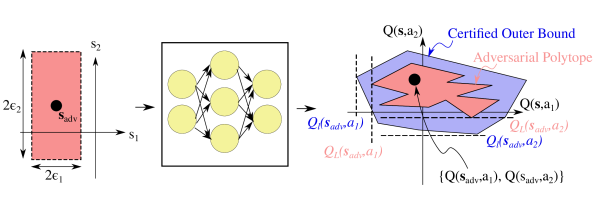
Figure 2: State Uncertainty Propagated Through Deep Q-Network. The red region (left) represents bounded state uncertainty (an $\ell_{\infty}\ \bm{\epsilon}$-ball) around the observed state, $\bm{s}_{\text{adv}}$. A neural network maps this set of possible inputs to a polytope (red) of possible outputs (Q-values in RL). This work’s extension of [27] provides an outer bound (blue) on that polytope. This work then modifies the RL action-selection rule by considering lower bounds, $Q_{l}$, on the blue region for each action. In this 2-state, 2-action example, our algorithm would select action 2, since $Q_{l}(\bm{s}_{\text{adv}},a_{2})>Q_{l}(\bm{s}_{\text{adv}},a_{1})$, i.e. the worst possible outcome from action 2 is better than the worst possible outcome from action 1, given an $\bm{\epsilon}$-ball uncertainty and a pre-trained DQN.

Deep RL

Many ideas from SL were transferred over to deep RL to provide empirical defenses to adversaries (e.g., training in adversarial environments [11, 12, 13, 14, 15], using model ensembles [12, 13]). Moreover, because adversarial observation perturbations are a form of measurement uncertainty, there are close connections between Safe RL [49] and adversarial robustness. Many Safe RL (also called risk-sensitive RL) algorithms optimize for the reward under worst-case assumptions of environment stochasticity, rather than optimizing for the expected reward [50, 51, 52]. The resulting policies are more risk-sensitive (i.e., robust to stochastic deviations in the input space, such as sensor noise), but could still fail on algorithmically crafted adversarial examples. In other words, modifying the RL training process to directly synthesize a provably robust neural network remains challenging.

Instead, this work adds a defense layer on top of an already trained DQN. We provide guarantees on the robustified policy’s solution quality by leveraging formal robustness analysis methods that propagate known DNN input bounds to guaranteed output bounds.

II-C Formal Robustness Methods

Although synthesis of a provably robust neural network is difficult, there is a closely related body of work that can provide other formal guarantees on network robustness – namely, a guarantee on how sensitive a trained network’s output is to input perturbations. The corresponding mathematical machinery to propagate an input set through a neural network allows for solving various robustness analysis problems, such as the calculation of reachable sets, minimal adversarial examples, or robustness verification.

For example, exact methods can be used to find tight bounds on the maximum network output deviation, given a nominal input and bounded input perturbation. These methods rely on Satisfiability Modulo Theory (SMT) [16, 17, 18], LP/mixed-integer LP solvers [19, 20], or zonotopes [21], to propagate constraints on the input space through to the output space (exactly). The difficulty in this propagation arises through DNN s with Rectified Linear Unit (ReLU)or other nonlinear activation functions – in fact, the problem of finding the exact output bounds is NP-complete (as shown by [17, 27]), making real-time implementations infeasible for many robotics tasks.

The formal robustness analysis approaches can be visualized in Fig. 2 in terms of a 2-state, 2-action deep RL problem. For a given state uncertainty set (red, left), the exact methods reason over the exact adversarial polytope (red, right), i.e., the image of the state uncertainty set through the network.

To enable scalable analysis, many researchers simultaneously proposed various relaxations of the NP-complete formulation: [29] provides a unifying framework of the convex relaxations that we briefly summarize here. A convex relaxation of the nonlinear activations enables the use of a standard LP solver to compute convex, guaranteed outer bounds, $Q_{LP}$, on the adversarial polytope (cf. Problem $\mathcal{C}$ in [29]). Even though this LP can be solved more efficiently than the exact problem with nonlinear activations, solving the relaxed LP is still computationally intensive.

Fortunately, the LP can be solved greedily, and thus even more efficiently, by using just one linear upper bound and one linear lower bound for each nonlinear layer. Several seemingly different approaches (e.g., solving the dual problem [22, 23, 24], using zonotopes/polyhedra as in [25, 26], using linear outer bounds [27, 28]) were shown to lead to very similar or identical network bounds in [29]. These greedy solutions provide over-approximations (see blue region in Fig. 2) on the LP solution and thus, also on the adversarial polytope. One of these methods, Fast-Lin [27] (which this work extends), can verify an image classification (MNIST) network’s sensitivity to perturbations for a given image in $<200ms$. As new approaches appear in the literature, such as [53], it will be straightforward to “upgrade” this work’s use of [27] for calculating lower bounds.

The analysis techniques described here in Section II-C are often formulated to solve the robustness verification problem: determine whether the calculated set of possible network outputs crosses a decision hyperplane (a line of slope 1 through the origin, in this example) – if it does cross, the classifier is deemed “not robust” to the input uncertainty. Our approach instead solves the robust decision-making problem: determine the best action considering worst-case outcomes, $Q_{l}(\bm{s}_{\text{adv}},a_{1}),Q_{l}(\bm{s}_{\text{adv}},a_{2})$, denoted by the dashed lines in Fig. 2.

II-D Certified Robustness in RL vs. SL

The inference phase of reinforcement learning (RL) and supervised learning (SL) are similar in that the policy chooses an action/class given some current input. However, there are at least three key differences between the proposed certified robustness for RL and existing certification methods for SL:

1. Existing methods for SL certification do not actually change the decision, they simply provide an additional piece of information (“is this decision sensitive to the set of possible inputs? yes/no/unsure”) alongside the nominal decision. Most SL certification papers do not discuss what to do if the decision is sensitive, which we identify as a key technical gap since in RL it is not obvious what to do with a sensitivity flag, as an action still needs to be taken. Thus, instead of just returning the nominal decision plus a sensitivity flag, the method in our paper makes a robust decision that considers the full set of inputs.

2. In SL, there is a “correct” output for each input (the true class label). In RL, the correct action is less clear because the actions need to be compared/evaluated in terms of their impact on the system. Furthermore, in RL, some actions could be much worse than others, whereas in SL typically all “wrong” outputs are penalized the same. Our method proposes using the Q-value encoded in a DNN as a way of comparing actions under state uncertainty.

3. In SL, a wrong decision incurs an immediate cost, but that decision does not impact the future inputs/costs. In RL, actions affect the system state, which does influence future inputs/rewards. This paper uses the value function to encode that information about the future, which we believe is an important first step towards considering feedback loops in the certification process.

To summarize, despite SL and RL inference appearing similarly, there are several key differences in the problem contexts that motivate a fundamentally different certification framework for RL.

III Background

III-A Preliminaries

In RL problems, the state-action value (or, “Q-value”)

$$Q(\bm{s},a)=\mathop{\mathbb{E}}_{\mathbf{s}^{\prime}\sim P}\left[\sum_{t=0}^{T}{\gamma^{t}r(t)}|\mathbf{s}(t{=}0)=\bm{s},\mathrm{a}(t{=}0)=a\right],$$

expresses the expected accumulation of future reward, $r$, discounted by $\gamma$, received by starting in state $\bm{s}\in\mathbb{R}^{n}$ and taking one of $d$ discrete actions, $a\in\{a_{0},a_{1},\ldots,a_{d-1}\}=\mathcal{A}$, with each next state $\mathbf{s}^{\prime}$ sampled from the (unknown) transition model, $P$. Furthermore, when we refer to Q-values in this work, we really mean a DNN approximation of the Q-values.

Let $\bm{\epsilon}\in\mathbb{R}^{n}_{\geq 0}$ be the maximum element-wise deviation of the state vector, and let $1\leq p\leq\infty$ parameterize the $\ell_{p}$-norm. We define the set of states within this deviation as the $\bm{\epsilon}$-Ball,

$$\mathcal{B}_{p}(\bm{s}_{0},\bm{\epsilon}) =\{\bm{s}:\lim_{\bm{\epsilon}^{\prime}\to\bm{\epsilon}^{+}}\lvert\lvert(\bm{s}-\bm{s}_{0})\oslash\bm{\epsilon}^{\prime}\rvert\rvert_{p}\leq 1\},$$ (1)

where $\oslash$ denotes element-wise division, and the $\mathrm{lim}$ is only needed to handle the case where $\exists i\ \epsilon_{i}=0$ (e.g., when the adversary is not allowed to perturb some component of the state, or the agent knows some component of the state vector with zero uncertainty).

An $\bm{\epsilon}$-Ball is illustrated in Fig. 3 for the case of $n=2$, highlighting that different elements of the state, $s_{i}$, might have different perturbation limits, $\epsilon_{i}$, and that the choice of $\ell_{p}$-norm affects the shape of the ball. The $\ell_{p}$-norm is defined as ${\lvert\lvert\bm{x}\rvert\rvert_{p}=(\lvert x_{1}\lvert^{p}+\ldots+\lvert x_{n}\lvert^{p})^{1/p}\ \mathrm{for}\ \bm{x}\in\mathbb{R}^{n},1\leq p\leq\infty}$.

Figure 3: Illustration of $\bm{\epsilon}$-Ball, $\mathcal{B}_{p}(\bm{s},\bm{\epsilon})$, for $n=2$. Let $\bm{\epsilon}=[\epsilon_{1},\epsilon_{2}]$. Depending on the choice of $\ell_{p}$ norm (e.g., $\ell_{1}$, $\ell_{2}$, and $\ell_{\infty}$), $\mathcal{B}_{p}(\bm{s},\bm{\epsilon})$ is the set of points inside the corresponding colored outline. The adversary can perturb nominal observation $\bm{s}$ to any point inside $\mathcal{B}_{p}(\bm{s},\bm{\epsilon})$. The values of $\{n,\bm{\epsilon},p\}$ are application-specific choices and the components of $\bm{\epsilon}$ need not be equal.

III-B Robustness Analysis

This work aims to find the action that maximizes state-action value under a worst-case perturbation of the observation by sensor noise or an adversary. This section explains how to efficiently obtain a lower bound on the DNN-predicted $Q$, given a bounded perturbation in the state space from the true state. The derivation is based on [27], re-formulated for RL.

The adversary perturbs the true state, $\bm{s}_{0}$, to another state, ${\bm{s}_{\text{adv}}\in\mathcal{B}_{p_{\text{adv}}}(\bm{s}_{0},\bm{\epsilon}_{\text{adv}})}$, within the $\bm{\epsilon}_{\text{adv}}$-ball. The ego agent only observes the perturbed state, ${\bm{s}_{\text{adv}}}$. As displayed in Fig. 2, let the worst-case state-action value, $Q_{L}$, for a given action, $a_{j}$, be

$$Q_{L}(\bm{s}_{\text{adv}},a_{j}) =\min_{\bm{s}\in\mathcal{B}_{p_{\text{adv}}}(\bm{s}_{\text{adv}},\bm{\epsilon}_{\text{adv}})}Q(\bm{s},a_{j}),$$ (2)

for all states $\bm{s}$ inside the $\bm{\epsilon}_{\text{adv}}$-Ball around the observation, $\bm{s}_{\text{adv}}$.

The goal of the analysis is to compute a guaranteed lower bound, $Q_{l}(\bm{s},a_{j})$, on the minimum state-action value, that is, $Q_{l}(\bm{s},a_{j})\leq Q_{L}(\bm{s},a_{j})$. The key idea is to pass interval bounds $[\bm{l}^{(0)},\bm{u}^{(0)}]=[\bm{s}_{\text{adv}}-\bm{\epsilon}_{\text{adv}},\bm{s}_{\text{adv}}+\bm{\epsilon}_{\text{adv}}]$ from the DNN’s input layer to the output layer, where $\bm{l}^{(k)}$ and $\bm{u}^{(k)}$ denote the lower and upper bounds of the pre-activation term, $\bm{z}^{(k)}$, i.e., $l_{i}^{(k)}{\leq}z_{i}^{(k)}{\leq}u_{i}^{(k)}\forall i\in{1,...,u_{k}}$, in the $k$-th layer with $u_{k}$ units of an $m$-layer DNN. When passing interval bounds through a ReLU activation, $\sigma(\cdot)$, the upper and lower pre-ReLU bounds of each element could either both be positive $(l_{r}^{(k)},u_{r}^{(k)}>0)$, negative $(l_{r}^{(k)},u_{r}^{(k)}<0)$, or positive and negative $(l_{r}^{(k)}<0,u_{r}^{(k)}>0)$, in which the ReLU status is called active, inactive or undecided, respectively. In the active and inactive case, bounds are passed directly to the next layer. In the undecided case, the output of the ReLU is bounded linearly above and below:

$$\sigma(z_{r}^{(k)})_{|l_{r}^{(k)},u_{r}^{(k)}}=\begin{cases}[z_{r}^{(k)},z_{r}^{(k)}]&\\ \quad\quad\text{if $l_{r}^{(k)},u_{r}^{(k)}>0$, ``active''}\vspace{0.1in}\\ [0,0]&\\ \quad\quad\text{if $l_{r}^{(k)},u_{r}^{(k)}<0$, ``inactive''}\vspace{0.1in}\\ [\frac{u_{r}^{(k)}}{u_{r}^{(k)}-l_{r}^{(k)}}z_{r}^{(k)},\frac{u_{r}^{(k)}}{u_{r}^{(k)}-l_{r}^{(k)}}(z_{r}^{(k)}-l_{r}^{(k)})]&\\ \quad\quad\text{if $l_{r}^{(k)}{<}0,u_{r}^{(k)}{>}0$, ``undecided'',}\end{cases}$$ (3)

for each element, indexed by $r$, in the $k$-th layer.

The identity matrix, $D$, is introduced as the ReLU status matrix, $H$ as the lower/upper bounding factor, $W$ as the weight matrix, $b$ as the bias in layer $(k)$ with $r$ or $j$ as indices, and the pre-ReLU-activation, $z_{r}^{(k)}$, is replaced with $W_{r,:}^{(k)}\bm{s}+b_{r}^{(k)}$. The ReLU bounding is then rewritten as

$$\begin{split}&\quad D_{r,r}^{(k)}(W_{r,j}^{(k)}s_{j}+b_{r}^{(k)})\\ \leq&\quad\sigma(W_{r,j}^{(k)}s_{j}+b_{r}^{(k)})\\ \leq&\quad D_{r,r}^{(k)}(W_{r,j}^{(k)}s_{j}+b_{r}^{(k)}-H_{r,j}^{(k)}),\end{split}$$ (4)

where

$$D_{r,r}^{(k)} =\begin{cases}1&\text{if $l_{r}^{(k)},u_{r}^{(k)}{>}0$;}\\ 0&\text{if $l_{r}^{(k)},u_{r}^{(k)}{<}0$,}\\ \frac{u_{r}^{(k)}}{u_{r}^{(k)}-l_{r}^{(k)}}&\text{if $l_{r}^{(k)}{<}0,u_{r}^{(k)}{>}0$;}\end{cases}$$ (5)

$$H_{r,j}^{(k)} =\begin{cases}l_{r}^{(k)}&\text{if $l_{r}^{(k)}{<}0,u_{r}^{(k)}{>}0,A_{j,r}^{(k)}{<}0$;}\\ 0&\text{otherwise.}\end{cases}$$ (6)

Using these ReLU relaxations, a guaranteed lower bound of the state-action value for a single state $\bm{s}\in\mathcal{B}_{p}(\bm{s}_{\text{adv}},\bm{\epsilon})$ (based on [27]) is:

$$\bar{Q}_{l}(\bm{s},a_{j})=A_{j,:}^{(0)}\bm{s}+b_{j}^{(m)}+\sum_{k=1}^{m-1}{A_{j,:}^{(k)}(\bm{b}^{(k)}-H_{:,j}^{(k)})},$$ (7)

where the matrix $A$ contains the network weights and ReLU activation, recursively for all layers: $A^{(k-1)}=A^{(k)}W^{(k)}D^{(k-1)}$, with identity in the final layer: $A^{(m)}=\mathds{1}$.

Unlike the exact DNN output, the bound on the relaxed DNN’s output in Eq. 7 can be minimized across an $\bm{\epsilon}$-ball in closed form (as described in Section IV-C), which is a key piece of this work’s real-time, robust decision-making framework.

IV Approach

This work develops an add-on, certifiably robust defense for existing Deep RL algorithms to ensure robustness against sensor noise or adversarial examples during test time.

IV-A System architecture

Figure 4: System Architecture. During online execution, an agent observes a state, $\bm{s}_{\text{adv}}$, corrupted by an adversary or noise process (constrained to $\bm{s}_{\text{adv}}\in\mathcal{B}_{p_{\text{adv}}}(\bm{s}_{0},\bm{\epsilon}_{\text{adv}})$. A trained Deep RL algorithm, e.g., DQN [54], predicts the state-action values, $Q$. The robustness analysis module computes a lower bound of the network’s predicted state-action values of each discrete action: $Q_{l}$, w.r.t. a robustness threshold $\bm{\epsilon}_{\text{rob}}$ and $\ell_{p_{\text{rob}}}$-norm in the input space. The agent takes the action, $a_{\text{CARRL}}$, that maximizes the lower bound, i.e., is best under a worst-case deviation in the input space, and returns a certificate bounding $a_{\text{CARRL}}$’s sub-optimality.

In an offline training phase, an agent uses a deep RL algorithm, here DQN [54], to train a DNN that maps non-corrupted state observations, $\bm{s}_{0}$, to state-action values, $Q(\bm{s}_{0},a)$. Action selection during training uses the nominal cost function, $a^{*}_{\text{nom}}=\operatorname*{\arg\!\max}_{a_{j}}Q(\bm{s}_{0},a_{j})$.

Figure 4 depicts the system architecture of a standard model-free RL framework with the added-on robustness module. During online execution, the agent only receives corrupted state observations from the environment. The robustness analysis node uses the DNN architecture, DNN weights, $W$, and robustness hyperparameters, $\bm{\epsilon}_{\text{rob}},p_{\text{rob}}$, to compute lower bounds on possible Q-values for robust action selection.

IV-B Optimal cost function under worst-case perturbation

We assume that the training process causes the network to converge to the optimal value function, $Q^{*}(\bm{s}_{0},a)$ and focus on the challenge of handling perturbed observations during execution. Thus, we consider robustness to an adversary that perturbs the true state, $\bm{s}_{0}$, within a small perturbation, $\bm{\epsilon}_{\text{adv}}$, into the worst-possible state observation, $\bm{s}_{\text{adv}}$. The adversary assumes that the RL agent follows a nominal policy (as in, e.g., DQN) of selecting the action with highest Q-value at the current observation. A worst possible state observation, $\bm{s}_{\text{adv}}$, is therefore any one which causes the RL agent to take the action with lowest Q-value in the true state, $\bm{s}_{0}$:

$$\bm{s}_{\text{adv}}\in\{\bm{s}:\; \bm{s}\in\mathcal{B}_{p_{\text{adv}}}(\bm{s}_{0},\bm{\epsilon}_{\text{adv}})\,\text{and}\,$$

$$\operatorname*{\arg\!\max}_{a_{j}}Q(\bm{s},a_{j})=\operatorname*{\arg\!\min}_{a_{j}}Q(\bm{s}_{0},a_{j})\}.$$ (8)

This set could be computationally intensive to compute and/or empty – an approximation is described in Section IV-H.

After the agent receives the state observation picked by the adversary, the agent selects an action. Instead of trusting the observation (and thus choosing the worst action for the true state), the agent could leverage the fact that the true state, $\bm{s}_{0}$, must be somewhere inside an $\bm{\epsilon}_{\text{adv}}$-Ball around $\bm{s}_{\text{adv}}$ (i.e., ${\bm{s}_{0}\in\mathcal{B}_{p_{\text{adv}}}(\bm{s}_{\text{adv}},\bm{\epsilon}_{\text{adv}}))}$.

However, in this work, the agent assumes ${\bm{s}_{0}\in\mathcal{B}_{p_{\text{rob}}}(\bm{s}_{\text{adv}},\bm{\epsilon}_{\text{rob}}))}$, where we make a distinction between the adversary and robust agent’s parameters. This distinction introduces hyperparameters $\bm{\epsilon}_{\text{rob}},\,p_{\text{rob}}$ that provide further flexibility in the defense algorithm’s conservatism, that do not necessarily have to match what the adversary applies. Nonetheless, for the sake of providing guarantees, the rest of Section IV assumes ${\bm{\epsilon}_{\text{rob}}=\bm{\epsilon}_{\text{adv}}}$ and ${p_{\text{rob}}=p_{\text{adv}}}$ to ensure ${\mathcal{B}_{p_{\text{rob}}}(\bm{s}_{\text{adv}},\bm{\epsilon}_{\text{rob}}))=\mathcal{B}_{p_{\text{adv}}}(\bm{s}_{\text{adv}},\bm{\epsilon}_{\text{adv}}))}$. Empirical effects of tuning ${\bm{\epsilon}_{\text{rob}}}$ to other values are explored in Section V.

The agent evaluates each action by calculating the worst-case Q-value under all possible true states.

Definition IV.1.

In accordance with the robust decision making problem, the robust-optimal action, $a^{*}$, is defined here as one with the highest Q-value under the worst-case perturbation,

$$a^{*}=\operatorname*{\arg\!\max}_{a_{j}}\underbrace{\min_{\bm{s}\in\mathcal{B}_{p_{\text{rob}}}(\bm{s}_{\text{adv}},\bm{\epsilon}_{\text{rob}})}Q(\bm{s},a_{j})}_{Q_{L}(\bm{s}_{\text{adv}},a_{j})}.$$ (9)

As described in Section II, computing $Q_{L}(\bm{s}_{\text{adv}},a_{j})$ exactly is too computationally intensive for real-time decision-making.

Thus, this work proposes the algorithm Certified Adversarial Robustness for Deep RL (CARRL).

Definition IV.2.

In CARRL, the action, $a_{\text{CARRL}}$, is selected by approximating $Q_{L}(\bm{s}_{\text{adv}},a_{j})$ with $Q_{l}(\bm{s}_{\text{adv}},a_{j})$, its guaranteed lower bound across all possible states $\bm{s}\in\mathcal{B}_{p_{\text{rob}}}(\bm{s}_{\text{adv}},\bm{\epsilon}_{\text{rob}})$, so that:

$$a_{\text{CARRL}}=\operatorname*{\arg\!\max}_{a_{j}}Q_{l}(\bm{s}_{\text{adv}},a_{j}),$$ (10)

where Eq. 16 below defines $Q_{l}(\bm{s}_{\text{adv}},a_{j})$ in closed form.

Conditions for optimality (${a^{*}=a_{\text{CARRL}}}$) are described in Section IV-D.

IV-C Robustness certification with vector-$\mathbf{\epsilon}$-ball perturbations

To solve Eq. 10 when $Q(\bm{s},a_{j})$ is represented by a DNN, we adapt the formulation from [27]. Most works in adversarial examples, including [27], focus on perturbations on image inputs, in which all channels have the same scale (e.g., grayscale images with pixel intensities in $[0,255]$). More generally, however, input channels could be on different scales (e.g., joint torques, velocities, positions). Existing robustness analysis methods require choosing a scalar $\epsilon_{\text{rob}}$ that bounds the uncertainty across all input channels; in general, this could lead to unnecessarily conservative behavior, as some network inputs might be known with zero uncertainty, or differences in units could make uncertainties across channels incomparable. Hence, this work computes bounds on the network output under perturbation bounds specific to each network input channel, as described in a vector $\bm{\epsilon}_{\text{rob}}$ with the same dimension as $\bm{s}$.

To do so, we minimize $\bar{Q}_{l}(\bm{s},a_{j})$ across all states in ${\mathcal{B}_{p_{\text{rob}}}(\bm{s}_{\text{adv}},\bm{\epsilon}_{\text{rob}})}$, where $\bar{Q}_{l}(\bm{s},a_{j})$ was defined in Eq. 7 as the lower bound on the Q-value for a particular state ${\bm{s}\in\mathcal{B}_{p_{\text{rob}}}(\bm{s}_{\text{adv}},\bm{\epsilon}_{\text{rob}})}$. This derivation uses a vector $\bm{\epsilon}_{\text{rob}}$ (instead of scalar $\epsilon_{\text{rob}}$ as in [27]):

$$\begin{split}Q_{l}(\bm{s}_{\text{adv}},a_{j})&=\min_{\bm{s}\in\mathcal{B}_{p}(\bm{s}_{\text{adv}},\bm{\epsilon}_{\text{rob}})}\left(\vphantom{\sum_{a}^{b}}\bar{Q}_{l}(\bm{s},a_{j})\right)\end{split}$$ (11)

$$\begin{split}&=\min_{\bm{s}\in\mathcal{B}_{p}(\bm{s}_{\text{adv}},\bm{\epsilon}_{\text{rob}})}\left(\vphantom{\sum_{a}^{b}}A_{j,:}^{(0)}\bm{s}+\right.\\ &\quad\quad\quad\quad\left.\underbrace{b_{j}^{(m)}+\sum_{k=1}^{m-1}{A_{j,:}^{(k)}(\bm{b}^{(k)}-H_{:,j}^{(k)})}}_{=:\Gamma}\right)\end{split}$$ (12)

$$\begin{split}&=\min_{\bm{s}\in\mathcal{B}_{p}(\bm{s}_{\text{adv}},\bm{\epsilon}_{\text{rob}})}\left(A_{j,:}^{(0)}\bm{s}\right)+\Gamma\end{split}$$ (13)

$$\begin{split}&=\min_{\bm{y}\in\mathcal{B}_{p}(\bm{0},\bm{1})}\left(A_{j,:}^{(0)}(\bm{y}\odot\bm{\epsilon}_{\text{rob}})\right)+A_{j,:}^{(0)}\bm{s}_{\text{adv}}+\Gamma\end{split}$$ (14)

$$\begin{split}&=\min_{\bm{y}\in\mathcal{B}_{p}(\bm{0},\bm{1})}\left((\bm{\epsilon}_{\text{rob}}\odot A_{j,:}^{(0)})\bm{y}\right)+A_{j,:}^{(0)}\bm{s}_{\text{adv}}+\Gamma\end{split}$$ (15)

$$\begin{split}&=-\lvert\lvert\bm{\epsilon}_{\text{rob}}\odot A_{j,:}^{(0)}\rvert\rvert_{q}+A_{j,:}^{(0)}\bm{s}_{\text{adv}}+\Gamma,\end{split}$$ (16)

with $\odot$ denoting element-wise multiplication. From Eq. 11 to Eq. 12, we substitute in Eq. 7. From Eq. 12 to Eq. 13, we introduce the placeholder variable $\Gamma$ that does not depend on $\bm{s}$. From Eq. 13 to Eq. 14, we substitute ${\bm{s}:=\bm{y}\odot\bm{\epsilon}_{\text{rob}}+\bm{s}_{\text{adv}}}$, to shift and re-scale the observation to within the unit ball around zero, $\bm{y}\in\mathcal{B}_{p}(\bm{0},\bm{1})$. The maximization in Eq. 15 is equivalent to a $\ell_{q}$-norm in Eq. 16 by the definition of the dual norm $\lvert\lvert\bm{z}\rvert\rvert_{q}=\{\text{sup}\ \bm{z}^{T}\bm{y}:\lvert\lvert\bm{y}\rvert\rvert_{p}\leq 1\}$ and the fact that the $\ell_{q}$ norm is the dual of the $\ell_{p}$ norm for $p,q\in[1,\infty)$ (with ${1/p+1/q=1}$). Equation 16 is inserted into Eq. 10 to calculate the CARRL action in closed form.

Recall from Section II that the bound $Q_{l}$ is the greedy (one linear upper and lower bound per activation) solution of an LP that describes a DNN with ReLU activations. In this work, we refer to the full (non-greedy) solution to the primal convex relaxed LP as $Q_{LP}$ (cf. Problem $\mathcal{C}$, LP-All in [29]).

To summarize, the relationship between each of the Q-value terms is:

$$Q(\bm{s}_{\text{adv}},a_{j}) \geq Q_{L}(\bm{s}_{\text{adv}},a_{j})\geq Q_{LP}(\bm{s}_{\text{adv}},a_{j})\geq Q_{l}(\bm{s}_{\text{adv}},a_{j})$$ (17)

$$Q(\bm{s}_{\text{adv}},a_{j}) \geq\bar{Q}_{l}(\bm{s}_{\text{adv}},a_{j})\geq Q_{l}(\bm{s}_{\text{adv}},a_{j}).$$ (18)

IV-D Guarantees on Action Selection

IV-D1 Avoiding a Bad Action

Unlike the nominal DQN rule, which could be tricked to take an arbitrarily bad action, the robust-optimal decision-rule in Eq. 9 can avoid bad actions provided there is a better alternative in the $\bm{\epsilon}_{\text{rob}}$-Ball.

Claim 1: If for some $q^{\prime}$, $\exists\bm{s}^{\prime}\in\mathcal{B}_{p_{\text{rob}}}(\bm{s}_{\text{adv}},\bm{\epsilon}_{\text{rob}}),a^{\prime}$ s.t. $Q(\bm{s}^{\prime},a^{\prime})\leq q^{\prime}$ and $\exists a^{\prime\prime}$ s.t. $\forall\bm{s}\in\mathcal{B}_{p_{\text{rob}}}(\bm{s}_{\text{adv}},\bm{\epsilon}_{\text{rob}})\ Q(\bm{s},a^{\prime\prime})>q^{\prime}$, then $a^{*}\neq a^{\prime}$.

In other words, if action $a^{\prime}$ is sufficiently bad for some nearby state, $\bm{s}^{\prime}$, and at least one other action $a^{\prime\prime}$ is better for all nearby states, the robust-optimal decision rule will not select the bad action $a^{\prime}$ (but DQN might). This is because $Q_{L}(\bm{s}_{\text{adv}},a^{\prime})\leq q^{\prime}$, $Q_{L}(\bm{s}_{\text{adv}},a^{\prime\prime})>q^{\prime}\Rightarrow\operatorname*{\arg\!\max}_{a_{j}}Q_{L}(\bm{s}_{\text{adv}},a_{j})\neq a^{\prime}$.

IV-D2 Matching the Robust-Optimal Action

While Claim 1 refers to the robust-optimal action, the action returned by CARRL is the same as the robust-optimal action (returned by a system that can compute the exact lower bounds) under certain conditions,

$$\underbrace{\operatorname*{\arg\!\max}_{a_{j}}Q_{l}(\bm{s}_{\text{adv}},a_{j})}_{a_{\text{CARRL}}}\stackrel{{\scriptstyle?}}{{=}}\underbrace{\operatorname*{\arg\!\max}_{a_{j}}Q_{L}(\bm{s}_{\text{adv}},a_{j})}_{a^{*}}.$$ (19)

Claim 2: CARRL selects the robust-optimal action if the robustness analysis process satisfies $Q_{l}=g(Q_{L})$, where $g$ is a strictly monotonic function, where $Q_{l},Q_{L}$ are written without their arguments, $\bm{s}_{\text{adv}},a_{j}$. A special case of this conditions is when the analysis returns a tight bound, i.e., $Q_{l}(\bm{s}_{\text{adv}},a_{j})=Q_{L}(\bm{s}_{\text{adv}},a_{j})$. Using the Fast-Lin-based approach in this work, for a particular observation, confirmation that all of the ReLUs are “active” or “inactive” in Eq. 3 would provide a tightness guarantee.

In cases whereClaim 2 is not fulfilled, but Claim 1 is fulfilled, CARRL is not guaranteed to select the robust-optimal action, but will still reason about all possible outcomes, and empirically selects a better action than a nominal policy across many settings explored in Section V.

Note that when $\bm{\epsilon}_{\text{rob}}=\bm{0}$, no robustness is applied, so both the CARRL and robust-optimal decisions reduce to the DQN decision, since $Q_{l}(\bm{s}_{\text{adv}},a_{j})=Q_{L}(\bm{s}_{\text{adv}},a_{j})=Q(\bm{s}_{\text{adv}},a_{j})$.

Claim 3: CARRL provides a certificate of the chosen action’s sub-optimality,

$$0 \leq Q(\mathbf{s}_{0},\,a^{**})-Q(\mathbf{s}_{0},\,a_{\text{CARRL}})$$

$$\leq\underbrace{\left(\max_{a_{j}}Q_{u}(\mathbf{s}_{\text{adv}},\,a_{j})\right)-Q_{l}(\mathbf{s}_{\text{adv}},\,a_{\text{CARRL}})}_{\text{Sub-optimality Certificate}},$$ (20)

where $a^{**}=\max_{a_{j}}Q(\mathbf{s}_{0},\,a_{j})$, i.e., the Q-maximizing action for the true (unknown) state, and $Q_{u}$ is an upper bound on $Q$ computed analogously to $Q_{l}$ in Eq. 16.

Proof.

The definition of $a^{**}$ implies $Q(\mathbf{s}_{0},\,a^{**})\geq Q(\mathbf{s}_{0},\,a_{j})$ for any $a_{j}\in\mathcal{A}$, including $a_{j}=a_{\text{CARRL}}$. This proves the lower bound.

For any $a_{j}\in\mathcal{A}$ including $a_{j}=a_{\text{CARRL}}$, the upper bound analog of Eq. 17 gives $Q_{u}(\mathbf{s}_{\text{adv}},\,a_{j})\geq{Q_{U}(\mathbf{s}_{\text{adv}},\,a_{j})=\max_{\mathbf{s}\in\mathcal{B}_{p_{\text{rob}}}(\bm{s}_{\text{adv}},\bm{\epsilon}_{\text{rob}})}Q(\mathbf{s},\,a_{j})\geq Q(\mathbf{s}_{0},\,a_{j})}$. Using the definition of $a^{**}$ thus gives ${\max_{a_{j}}Q_{u}(\mathbf{s}_{\text{adv}},\,a_{j})\geq\max_{a_{j}}Q(\mathbf{s}_{0},\,a_{j})=Q(\mathbf{s}_{0},\,a^{**})}$. Using Eqs. 17 and 9, ${Q_{l}(\mathbf{s}_{\text{adv}},\,a_{j})\leq Q_{L}(\mathbf{s}_{\text{adv}},\,a_{j})\leq Q_{l}(\mathbf{s}_{0},\,a_{j})}$, because $\mathbf{s}_{0}\in\mathcal{B}_{p_{\text{rob}}}(\bm{s}_{\text{adv}},\bm{\epsilon}_{\text{rob}})$. This proves the upper bound. ∎

The benefit of Eq. 20 is that it bounds the difference in the Q-value of CARRL’s action under input uncertainty and the action that would have been taken given knowledge of the true state. Thus, the bound in Eq. 20 captures the uncertainty in the true state (considering the whole $\mathbf{\epsilon}$-ball through $Q_{u},Q_{l}$), and the unknown action $a^{**}$ that is optimal for the true (unknown) state.

This certificate of sub-optimality is what makes CARRL certifiably robust, with further discussion in Certified vs. Verified Terminology.

IV-E Probabilistic Robustness

The discussion so far considered cases where the state perturbation is known to be bounded (as in, e.g., many adversarial observation perturbation definitions [31], stochastic processes with finite support. However, in many other cases, the observation uncertainty is best modeled by a distribution with infinite support (e.g., Gaussian). To be fully robust to this class of uncertainty (including very low probability events) CARRL requires setting $\epsilon_{rob,i}=\infty$ for the unbounded state elements, $\bm{s}_{i}$.

For instance, for a Gaussian sensor model with known standard deviation of measurement error, $\bm{\sigma}_{sensor}$, one could set ${\bm{\epsilon}_{\text{rob}}=2\bm{\sigma}_{sensor}}$ to yield actions that account for the worst-case outcome with 95% confidence. In robotics applications, for example, $\bm{\sigma}_{sensor}$ is routinely provided in a sensor datasheet. Implementing this type of probabilistic robustness only requires a sensor model for the observation vector and a desired confidence bound to compute the corresponding $\bm{\epsilon}_{\text{rob}}$.

IV-F Design of a Policy with Reduced Sensitivity

While Eq. 9 provides a robust policy by selecting an action with best worst-case performance, an alternative robustness paradigm could prefer actions with low sensitivity to changes in the input while potentially sacrificing performance. Using the same machinery as before to compute guaranteed output bounds per action, we add a cost term to penalize sensitivity. This interpretation gives a reduced sensitivity (RS) action-selection rule,

$$a^{*}_{\text{RS}} =\operatorname*{\arg\!\max}_{a_{j}}\left[\underbrace{Q_{L}(\bm{s}_{\text{adv}},a_{j})}_{\text{Worst-Case Performance}}-\right.$$ (21)

$$\quad\quad\left.\lambda_{\text{sens}}\cdot\underbrace{\left(Q_{U}(\bm{s}_{\text{adv}},a_{j})-Q_{L}(\bm{s}_{\text{adv}},a_{j})\right)}_{\text{Sensitivity}}\right],$$

where $Q_{U}$ is defined analogously to $Q_{L}$ in Eq. 9 and $\lambda_{\text{sens}}$ is a hyperparameter to trade-off nominal performance and sensitivity. In practice, guaranteed bounds $Q_{u},\,Q_{l}$ can be used instead of $Q_{U},\,Q_{L}$ in Eq. 21 for a coarser estimate of action sensitivity.

The benefit of the formulation in Eq. 21 is that it penalizes actions with a wide range of possible Q-values for the input set, while still considering worst-case performance. That is, an action with a wide range of possible Q-values will be less desirable than in the previous robust action-selection rule in Eq. 9. In the two extremes, $\lambda_{\text{sens}}=0\implies a^{*}_{\text{RS}}=a^{*}$; whereas $\lambda_{\text{sens}}\to\infty\implies a^{*}_{\text{RS}}$ ignores performance and always chooses action that is least sensitive to input changes.

IV-G Robust Policy-Based RL

There are two main classes of RL methods: value-function-based and policy-based. The preceding sections introduce robustness methods for value-function-based RL algorithms, such as DQN [41]. The other main class of RL methods instead learn a policy distribution directly, with or without simultaneously learning to estimate the value function (e.g., A3C [55], PPO [56], SAC [57]). Here we show that the proposed robust optimization formulation can be adapted to policy-based RL with discrete actions.

For example, consider the Soft Actor-Critic (SAC) [57] algorithm (extended to discrete action spaces [58]). After training, SAC returns a DNN policy. We can use the trained policy logits as an indication of desirability for taking an action (last layer before softmax/normalization). Let the logits be denoted as $\mu(\cdot\lvert\bm{s})\in\mathbb{R}^{d}$ and the policy distribution be $\pi(\cdot\lvert\bm{s})=\mathrm{softmax}(\mu(\cdot\lvert\bm{s}))\in\Delta^{d}$, where $\Delta^{d}$ denotes the standard $d$-simplex.

In accordance with the robust decision making problem, the robust-optimal action, $a^{*}_{\pi}$, is defined here as one with the highest policy logit under the worst-case perturbation,

$$a^{*}_{\pi}=\operatorname*{\arg\!\max}_{a_{j}}\underbrace{\min_{\bm{s}\in\mathcal{B}_{p_{\text{rob}}}(\bm{s}_{\text{adv}},\bm{\epsilon}_{\text{rob}})}\mu(a_{j}\lvert\bm{s})}_{\mu_{L}(a_{j}\lvert\bm{s}_{\text{adv}})}.$$ (22)

Our computationally tractable implementation selects $a_{\text{CARRL},\pi}$ by approximating $\mu_{L}(a_{j}\lvert\bm{s}_{\text{adv}})$ with $\mu_{l}(a_{j}\lvert\bm{s}_{\text{adv}})$, its guaranteed lower bound across all possible states $\bm{s}\in\mathcal{B}_{p_{\text{rob}}}(\bm{s}_{\text{adv}},\bm{\epsilon}_{\text{rob}})$, so that:

$$a_{\text{CARRL},\pi}=\operatorname*{\arg\!\max}_{a_{j}}\mu_{l}(a_{j}\lvert\bm{s}_{\text{adv}}),$$ (23)

where $\mu_{l}(a_{j}\lvert\bm{s}_{\text{adv}})$ can be computed in closed form using Eq. 16, where the only modification is the interpretation of the DNN output (Q-value vs. policy logits).

The robust, deterministic policy returned by this formulation applies to several standard RL methods, including [57, 59]. If a stochastic policy is preferred for other RL algorithms, one could sample from the normalized lower bounded logits, i.e., $a_{\text{CARRL},\pi}\sim\mathrm{softmax}(\mu_{l}(\cdot\lvert\bm{s}_{\text{adv}}))$. Because of the similarity in formulations for robust policy-based and value-function-based RL, DQN is used as a representative example going forward.

IV-H Adversaries

To evaluate the learned policy’s robustness to deviations of the input in an $\bm{\epsilon}_{\text{adv}}$-Ball, we pass the true state, $\bm{s}_{0}$, through an adversarial/noise process to compute $\bm{s}_{\text{adv}}$, as seen in Fig. 4. Computing an adversarial state $\bm{s}_{\text{adv}}$ exactly, using Eq. 8, is computationally intensive. Instead, we use a Fast Gradient Sign method with Targeting (FGST) [8] to approximate the adversary from Eq. 8 (other adversaries could include PGD [39], ZOO [60]). FGST chooses a state $\hat{\bm{s}}_{\text{adv}}$ on the ${\ell_{\infty}\ \bm{\epsilon}_{\text{adv}}}$-Ball’s perimeter to encourage the agent to take the nominally worst action, $\operatorname*{\arg\!\min}_{a_{j}}Q(\bm{s}_{0},a_{j})$. Specifically, $\hat{\bm{s}}_{\text{adv}}$ is picked along the direction of sign of the lowest cross-entropy loss, $\mathcal{L}$, between $\bm{y}_{\text{adv}}$, a one-hot encoding of the worst action at $\bm{s}_{0}$, and $\bm{y}_{\text{nom}}$, the softmax of all actions’ Q-values at $\bm{s}_{0}$. The loss is taken w.r.t. the proposed observation $\bm{s}$:

$$\bm{y}_{\text{adv}} =[\mathds{1}\{a_{i}={\mathop{\mathrm{argmin}}\nolimits}_{a_{j}}Q(\bm{s}_{0},a_{j})\}]\in\mathbbm{U}^{d}$$ (24)

$$Q_{\text{nom}} =[Q(\bm{s}_{0},a_{j})\forall j\in\{0,\ldots,d-1\}]\in\mathbb{R}^{d}$$ (25)

$$\bm{y}_{\text{nom}} =\mathrm{softmax}(Q_{\text{nom}})\in\Delta^{d}$$ (26)

$$\hat{\bm{s}}_{\text{adv}} =\bm{s}_{0}-\bm{\epsilon}_{\text{adv}}\odot\mathrm{sign}(\nabla_{\bm{s}}\mathcal{L}(\bm{y}_{\text{adv}},\bm{y}_{\text{nom}})),$$ (27)

where $\mathbbm{U}^{d}$ denotes a one-hot vector of dimension $d$, and $\Delta^{d}$ denotes the standard $d$-simplex.

In addition to adversarial perturbations, Section V also considers uniform noise perturbations, where ${\bm{s}_{\text{adv}}\sim\mathtt{Unif}\left(\left[\bm{s}_{0}-\bm{\sigma},\bm{s}_{0}+\bm{\sigma}\right]\right)}$.

V Experimental Results

(a) $\epsilon_{\text{rob}}=0.0$

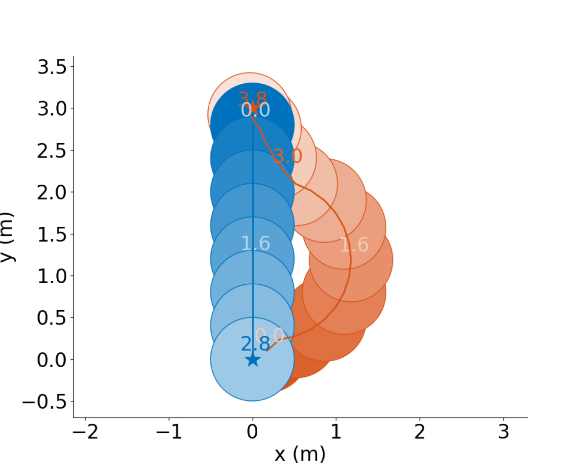
(b) $\epsilon_{\text{rob}}=0.1$

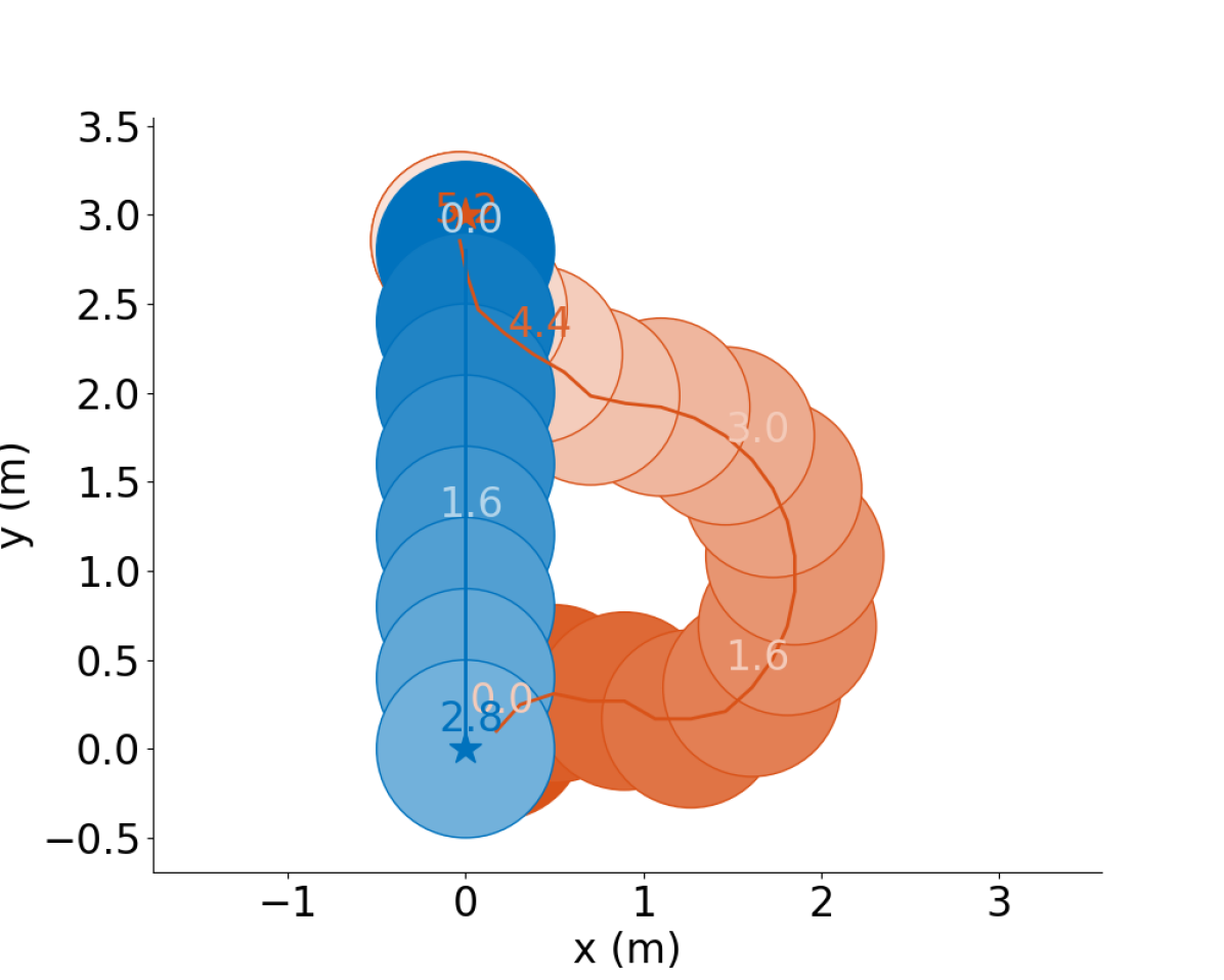
(c) $\epsilon_{\text{rob}}=0.46$

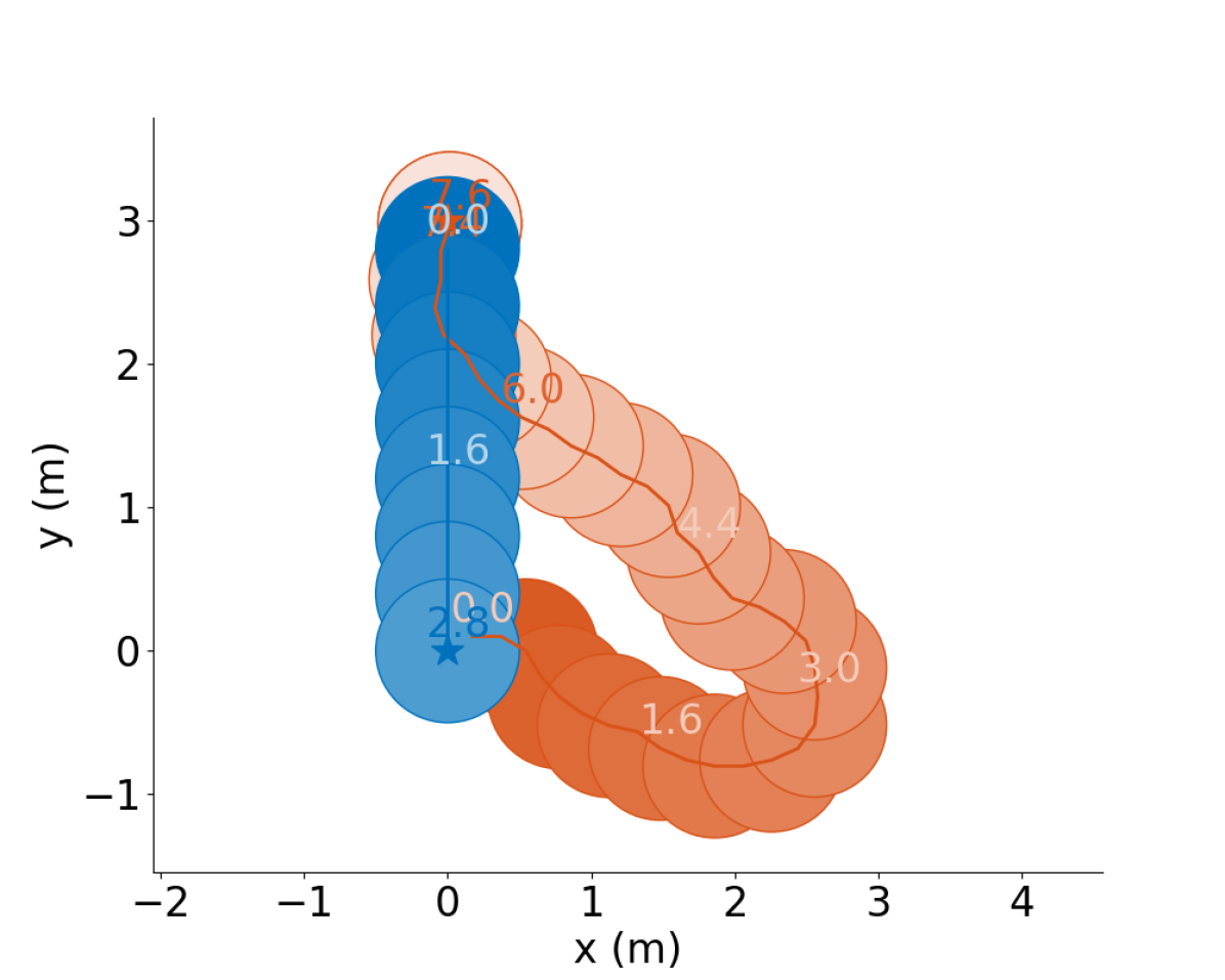
(d) $\epsilon_{\text{rob}}=1.0$

(e) $\epsilon_{\text{rob}}=2.0$

Figure 5: Increase of conservatism with $\epsilon_{\text{rob}}$. An agent (orange) following the CARRL policy avoids a dynamic, non-cooperative obstacle (blue) that is observed without noise. An increasing robustness parameter $\epsilon_{\text{rob}}$ (left to right) increases the agent’s conservatism, i.e., the agent avoids the obstacle with a greater safety distance.

(a)

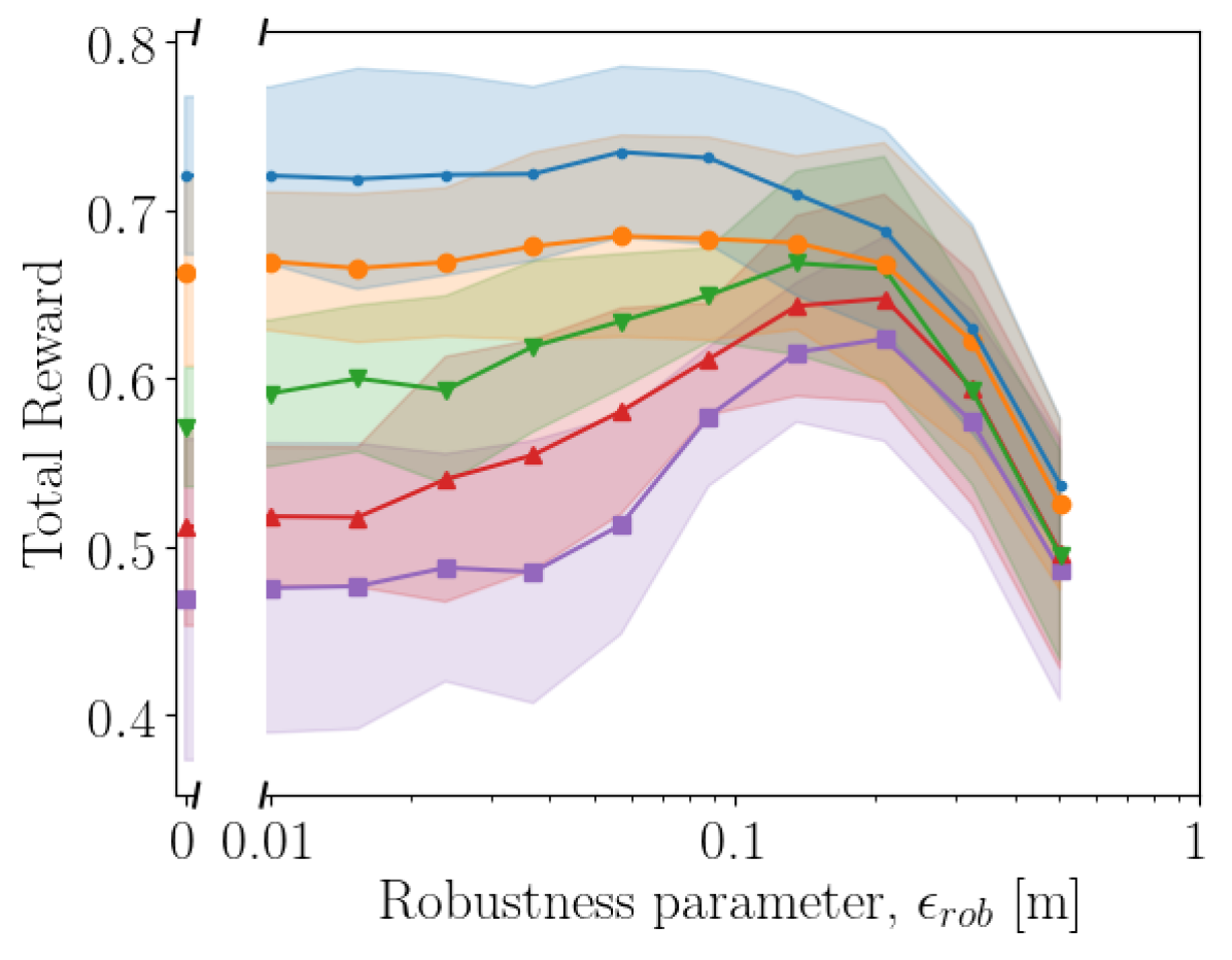
(b)

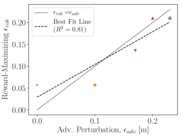
(c)

(d)

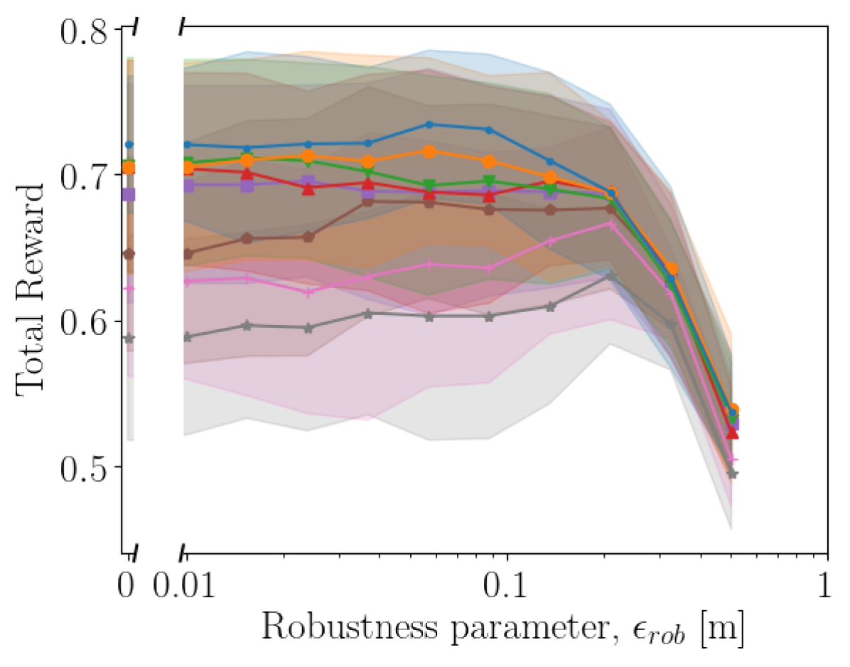
(e)

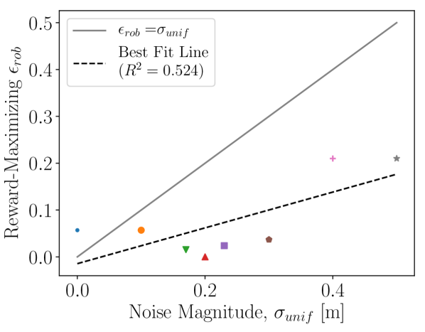
(f)

Figure 6: Robustness against adversarial attacks (top row) and noise (bottom row). Increasing the robustness parameter, $\epsilon_{\text{rob}}$, decreases the number of collisions in the presence of adversarial attacks (a), or noise (d) for various perturbation magnitudes, $\epsilon_{\text{adv}},\sigma_{\text{unif}}$. CARRL also recovers substantial amounts of reward lost due to imperfect observations as $\epsilon_{\text{rob}}$ increases (b,e). The choice of $\epsilon_{\text{rob}}$ to maximize reward in the presence of a particular adversary or noise process can be guided by the models in (c,f). When $\epsilon_{\text{rob}}=0$, CARRL is equivalent to DQN.

The key result is that while imperfect observations reduce the performance of a nominal deep RL algorithm, our proposed algorithm, CARRL, recovers much of the performance by adding robustness during execution. Robustness against perturbations from an adversary or noise process during execution is evaluated in two simulated domains: collision avoidance among dynamic, decision-making obstacles [61] and cartpole [62]. This section also describes the impact of the $\bm{\epsilon}_{\text{rob}}$ hyperparameter, the ability to handle behavioral adversaries, a comparison with another analysis technique, and provides intuition on the tightness of the lower bounds.

V-A Collision Avoidance Domain

Among the many RL tasks, a particularly challenging safety-critical task is collision avoidance for a robotic vehicle among pedestrians. Because learning a policy in the real world is dangerous and time consuming, this work uses a gym-based [62] kinematic simulation environment [61] for learning pedestrian avoidance policies. In this work, the RL policy controls one of two agents with 11 discrete actions: change of heading angle evenly spaced between $[-\pi/6,+\pi/6]$ and constant velocity $v=1$ m/s. The environment executes the selected action under unicycle kinematics, and controls the other agent from a diverse set of fixed policies (static, non-cooperative, ORCA [63], GA3C-CADRL [4]). The sparse reward is $1$ for reaching the goal, $-0.25$ for colliding (and 0 otherwise, i.e., zero reward is received in cases where the agent does not reach its goal in a reasonable amount of time). The observation vector includes the CARRL agent’s goal, each agent’s radius, and the other agent’s x-y position and velocity, with more detail in [4]. In this domain, robustness and perturbations are applied only on the measurement of the other agent’s x-y position (i.e., ${\bm{\epsilon}_{\text{rob}}=\epsilon_{\text{rob}}\cdot\left[0\ \ldots\ 0\ 1\ 1\ 0\ \ldots 0\right]}$) – an example of CARRL’s ability to handle uncertainties of varying scales.

A non-dueling DQN policy was trained with $2$, $64$-unit layers with the following hyperparameters: learning rate $2.05\texttt{e}{-4}$, $\epsilon$-greedy exploration ratio linearly decaying from $0.5$ to $0.05$, buffer size $152\texttt{e}3$, $4\texttt{e}5$ training steps, and target network update frequency, $10\texttt{e}3$. The hyperparameters were found by running 100 iterations of Bayesian optimization with Gaussian Processes [64] on the maximization of the sparse training reward.

After training, CARRL is added onto the trained DQN policy. Intuition on the resulting CARRL policy is demonstrated in Fig. 5. The figure shows the trajectories of the CARRL agent (orange) for increasing $\epsilon_{\text{rob}}$ values in a scenario with unperturbed observations. With increasing $\epsilon_{\text{rob}}$ (toward right), the CARRL agent accounts for increasingly large worst-case perturbations of the other agent’s position. Accordingly, the agent avoids the dynamic agent (blue) increasingly conservatively, i.e., selects actions that leave a larger safety distance. When $\epsilon_{\text{rob}}{=}2.0$, the CARRL agent is overly conservative – it “runs away” and does not reach its goal, which is explained more in Section V-G.

Figure 6 shows that the nominal DQN policy is not robust to the perturbation of inputs. In particular, increasing the magnitude of adversarial, or noisy perturbation, $\epsilon_{\text{adv}},\sigma_{\text{unif}}$, drastically 1) increases the average number of collisions (as seen in Figs. 6 and 6, respectively, at $\epsilon_{\text{rob}}=0$) and 2) decreases the average reward (as seen in Figs. 6 and 6). The results in Fig. 6 are evaluated in scenarios where the other agent is non-cooperative (i.e., travels straight to its goal position at constant velocity) and each datapoint represents the average of 100 trials across 5 random seeds that determine the agents’ initial/goal positions and radii (shading represents $\pm 1$ standard deviation of average value per seed).

Next, we demonstrate that CARRL recovers performance. Increasing the robustness parameter $\epsilon_{\text{rob}}$ decreases the number of collisions under varying magnitudes of noise, or adversarial attack, as seen in Figs. 6 and 6. Because collisions affect the reward function, the received reward also increases with an increasing robustness parameter $\epsilon_{\text{rob}}{<}{\sim}0.1$ under varying magnitudes of perturbations. As expected, the effect of the proposed defense is highest under large perturbations, as seen in the slopes of the curves $\epsilon_{\text{adv}}{=}0.23$ (violet) and $\sigma_{\text{unif}}{=}0.5$ (gray).

Since the CARRL agent selects actions more conservatively than a nominal DQN agent, it is able to successfully reach its goal instead of colliding like a nominal DQN agent does under many scenarios with noisy or adversarial perturbations. However, the effect of overly conservative behavior seen in Figs. 5 and 5 appears in Fig. 6 for $\epsilon_{\text{rob}}{>}\sim 0.2$, as the reward drops significantly. This excessive conservatism for large $\bm{\epsilon}_{\text{rob}}$ can be partially explained by the fact that highly conservative actions may move the agent’s position observation into states that are far from what the network was trained on, which breaks CARRL’s assumption of a perfectly learned Q-function. Further discussion about the conservatism inherent in the lower bounds is discussed in Section V-G.

Figures 6 and 6 illustrate further intuition on choosing $\epsilon_{\text{rob}}$. Figure 6 demonstrates a strong correlation between the attack magnitude $\epsilon_{\text{adv}}$ and the best (i.e., reward-maximizing) robustness hyperparameter $\epsilon_{\text{rob}}$ under that attack magnitude from Fig. 6. In the case of uniform noise, the correlation between $\epsilon_{\text{rob}}$ and $\sigma_{\text{unif}}$ is weaker, because the FGST adversary chooses an input state on the perimeter of the $\bm{\epsilon}_{\text{adv}}$-Ball, whereas uniform noise samples lie inside the $\bm{\sigma}_{unif}$-Ball.

The flexibility in setting $\epsilon_{\text{rob}}$ enables CARRL to capture uncertainties of various magnitudes in the input space, e.g., $\epsilon_{\text{rob}}$ could be adapted on-line to account for a perturbation magnitude that is unknown a priori, or to handle time-varying sensor noise.

V-B Cartpole Domain

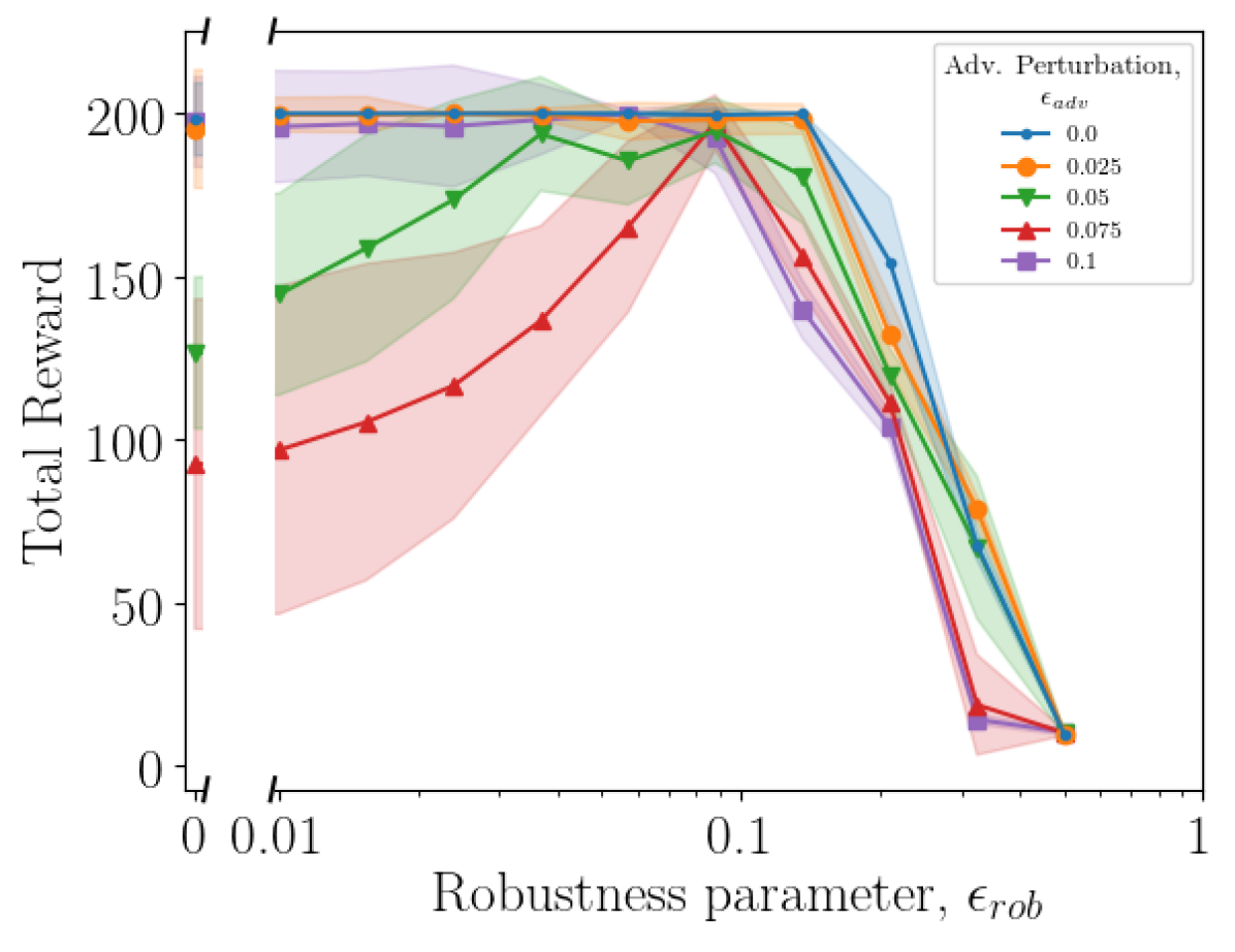
(a) Robustness to Adversaries (Cartpole)

(b) Choosing $\epsilon_{\text{rob}}$ in Presence of Adversary (Cartpole)

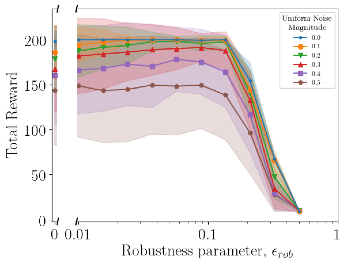
(c) Robustness to Sensor Noise (Cartpole)

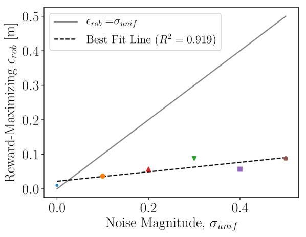
(d) Choosing $\epsilon_{\text{rob}}$ in Presence of Noise (Cartpole)

Figure 7: Results on Cartpole. CARRL recovers performance (measured by reward received) by adding robustness under various magnitudes of adversarial (a) and uniform noise (c) perturbations. Each curve in (a,c) correspond to a different magnitude of perturbation, and $\epsilon_{\text{rob}}=0$ corresponds to zero robustness, i.e., DQN. For all adversary/noise magnitudes, CARRL becomes overly conservative for large $\epsilon_{\text{rob}}$, and the performance degrades. Thus, choosing the best $\epsilon_{\text{rob}}$ for a particular perturbation magnitude can be guided by the curves in (b,d).

In the cartpole task [65, 62], the reward is the number of time steps (capped at $200$) that a pole remains balanced upright ($\pm 12^{\circ}$ from vertical) on a cart that can translate along a horizontal track. The state vector, ${\bm{s}=\left[p_{cart},v_{cart},\theta_{pole},\dot{\theta}_{pole}\right]^{T}}$ and action space, ${\bm{a}\in\{\mathrm{push\ cart\ left},\mathrm{push\ cart\ right}\}}$ are defined in [62]. A $2$-layer, $4$-unit network was trained in an environment without any observation perturbations using an open-source DQN implementation [66] with Bayesian Optimization used to find training hyperparameters. The trained DQN is evaluated against perturbations of various magnitudes, shown in Fig. 7. In this domain, robustness and perturbations are applied to all states equally, i.e., ${\bm{\epsilon}_{\text{adv}}=\epsilon_{\text{adv}}\cdot\mathbbm{1}\in\mathbbm{R}^{4}}$, ${\bm{\epsilon}_{\text{rob}}=\epsilon_{\text{rob}}\cdot\mathbbm{1}\in\mathbbm{R}^{4}}$ and ${\bm{\sigma}_{unif}=\sigma_{unif}\cdot\mathbbm{1}\in\mathbbm{R}^{4}}$.

Each curve in Figs. 7 and 7 corresponds to the average reward received under different magnitudes of adversarial, or uniform noise perturbations, respectively. The reward of a nominal DQN agent drops from $200$ under perfect measurements to $105$ under adversarial perturbation of magnitude $\epsilon_{\text{adv}}=0.075$ (blue and red reward at x-axis, ${\epsilon_{\text{rob}}=0}$ in Fig. 7) or to $145$ under uniform noise of magnitude $\sigma_{\text{unif}}=0.5$ (Fig. 7). For $\epsilon_{\text{rob}}>0$ (moving right along x-axis), the CARRL algorithm considers an increasingly large range of states in its worst-case outcome calculation. Accordingly, the algorithm is able to recover some of the performance lost due to imperfect observations. For example, with $\epsilon_{\text{adv}}=0.075$ (red triangles), CARRL achieves 200 reward using CARRL with $\epsilon_{\text{rob}}=0.1$. The ability to recover performance is due to CARRL selecting actions that consider the worst-case state (e.g., a state in which the pole is closest to falling), rather than fully trusting the perturbed observations.

However, there is again tradeoff between robustness and conservatism. For large values of $\epsilon_{\text{rob}}$, the average reward declines steeply for all magnitudes of adversaries and noise, because CARRL considers an excessively large set of worst-case states (more detail provided in Section V-G).

The reward-maximizing choice of $\epsilon_{\text{rob}}$ for a particular class and magnitude of perturbations is explored in Figs. 7 and 7. Similarly to the collision avoidance domain, the best choice of $\epsilon_{\text{rob}}$ is close to $\epsilon_{\text{adv}}$ under adversarial perturbations and less than $\sigma_{\text{unif}}$ under uniform noise perturbations.

These results use 200 random seeds causing different initial conditions.

V-C Atari Pong Domain

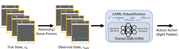
Figure 8: Adversary & Defense in Atari Pong. At each timestep, given the true state (the past 4 $210\times 160$ grayscale image frames), the adversary finds the pixels corresponding to the ball and moves them downward by $\epsilon_{\text{adv}}$ pixels. The CARRL algorithm enumerates the possible un-perturbed states, according to $\epsilon_{\text{rob}}$, re-shapes the observation to $(84,84,4)$, and makes a DQN forward pass to compute $Q_{L}$ from Eq. 9. The resulting robust-optimal action is implemented, which moves the environment to a new true state, and the cycle repeats.

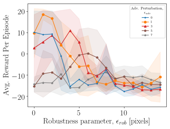
(a) Robustness to Adversaries (Atari Pong)

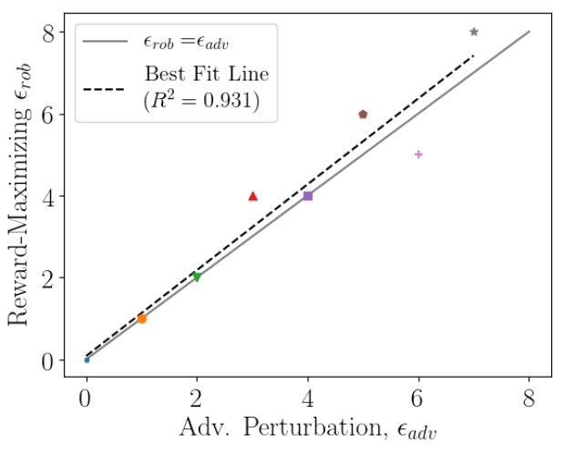
(b) Choosing $\epsilon_{\text{rob}}$ in Presence of Adversary (Atari Pong)

Figure 9: Results on Atari Pong. CARRL recovers performance (measured by reward received) by adding robustness under various magnitudes pixel perturbations. In (a), each curve corresponds to a different magnitude of perturbation, and $\epsilon_{\text{rob}}=0$ corresponds to zero robustness, i.e., DQN. For all adversary/noise magnitudes, CARRL recovers performance roughly until $\epsilon_{\text{rob}}=\epsilon_{\text{adv}}$, and then CARRL becomes overly conservative for large $\epsilon_{\text{rob}}$, and the performance degrades. To tune $\epsilon_{\text{rob}}$, (b) shows the reward-maximizing value of $\epsilon_{\text{rob}}$ is closely correlated with the (unknown) adversary’s magnitude, $\epsilon_{\text{adv}}$. Both (a, b) demonstrate similar behavior to that observed in collision avoidance and cartpole tasks, but on a high-dimensional task, with input vector of $(84,84,4)$ images and a more complicated DQN architecture (multi-layer CNN from [54]).

To evaluate CARRL on a task of high dimension, we implemented an adversary and robust defense in image space for the Atari Pong environment [67, 68]. The framework from [66, 69] enabled training a DQN on the standard PongNoFrameskip-v4 task. In this task, the observation vector has dimension $(84,84,4)$, which represents the past 4 screen frames as grayscale images, and agent chooses from 6 discrete actions to move the right paddle up/down (4 of the actions have no effect). In addition to a higher-dimensional input vector than in the prior domains (collision avoidance and cartpole), the DQN architecture [54] used for Pong, consisting of 3 convolutional layers, 2 fully connected layers, all with ReLU activations, is substantially more complicated than the DQNs used above.

Fig. 8 shows the adversary/defense architecture used in this work’s Pong experiments. The true state is shown on the left, as frames with dimension $(210,160,4)$. An adversary finds the ball in each frame by filtering based on pixel intensity and then shifts the pixels corresponding to the ball downward by the allowed magnitude, $\epsilon_{\text{adv}}$. The perturbation is limited to keep the ball within the playable area when the ball is near the perimeter.

This perturbation, if not accounted for, causes a nominal DQN agent act as if the ball is lower than it really is, which causes the agent to position its paddle too low and thus miss the ball and lose a point. Intuitively, given knowledge of the adversary’s magnitude allowance, the robust behavior should be to position the paddle in the middle of all possible ball positions to ensure the paddle at least strikes the ball.

Recall that the previous domains had continuous state spaces, which motivated the calculation of a lower bound, $Q_{l}$, on the worst-case Q-value. Because the Pong state space is discrete (pixels have integer values $\in[0,255]$), the calculation of $Q_{L}$ can be done exactly by enumerating possible states and querying the DQN for all possibilities in parallel. Thus, CARRL returns the robust-optimal action, $a^{*}$, from Eq. 9 in this domain. CARRL enumerates all possible states by shifting the ball position upward by each integer value $\in[0,\epsilon_{\text{rob}}]$, leading to $\epsilon_{\text{rob}}+1$ components of the DQN forward pass. Note that the adjusted perturbed observation is then downscaled into the $(84,84,4)$ vector for the DQN architecture, where the ball-moving operations are done in the raw $(210,160,4)$ images to avoid the complexities of blurring/interpolation when finding the ball pixels.

After designing the adversary/defense for this domain, we ran 50 games with various combinations of $\epsilon_{\text{rob}}$ and $\epsilon_{\text{adv}}$, as shown in Fig. 9. In Pong, the two players repeatedly play until one player reaches 21 points, and the reward returned by the environment at the end of an episode is the difference in the two players’ scores (e.g., lose $21-6$ $\Rightarrow$ $-15$ reward, and $|R|\leq 21$).

Fig. 9(a) shows similar behavior as in the other domains. When $\epsilon_{\text{rob}}=0$ (left-most points), the average reward decreases as the adversary’s strength increases (from 0 to 7 pixels). Then, as $\epsilon_{\text{rob}}$ is increased, the reward generally increases, then reaches a peak around $\epsilon_{\text{rob}}\approx\epsilon_{\text{adv}}$, then decreases because the agent is too conservative. Furthermore, Fig. 9(b) shows that the reward-maximizing choice of $\epsilon_{\text{rob}}$ is correlated with the adversary’s strength, $\epsilon_{\text{adv}}$. These results suggest that the proposed framework for robustification of learned policies can also be deployed in high-dimensional tasks, such as Pong, with high-dimensional CNNs, such as the DQN architecture from [54].

V-D Computational Efficiency

For the cartpole task, one forward pass with bound calculation takes on average $0.68\pm 0.06$ms, which compares to a forward pass of the same DQN (nominal, without calculating bounds) of $0.24\pm 0.03$ms; for collision avoidance, it takes $1.85\pm 1.62$ms (CARRL) and $0.30\pm 0.04$ms (DQN), all on one i7-6700K CPU. In our implementation, the bound of all actions (i.e., 2 or 11 discrete actions for the cartpole and collision avoidance domain, respectively) are computed in parallel. While the DQN s used in this work are relatively small, [27] shows that the runtime of Fast-Lin scales linearly with the network size, and a recent GPU implementation offers faster performance [70], suggesting CARRL could be implemented in real-time for higher-dimensional RL tasks, as well.

V-E Robustness to Behavioral Adversaries

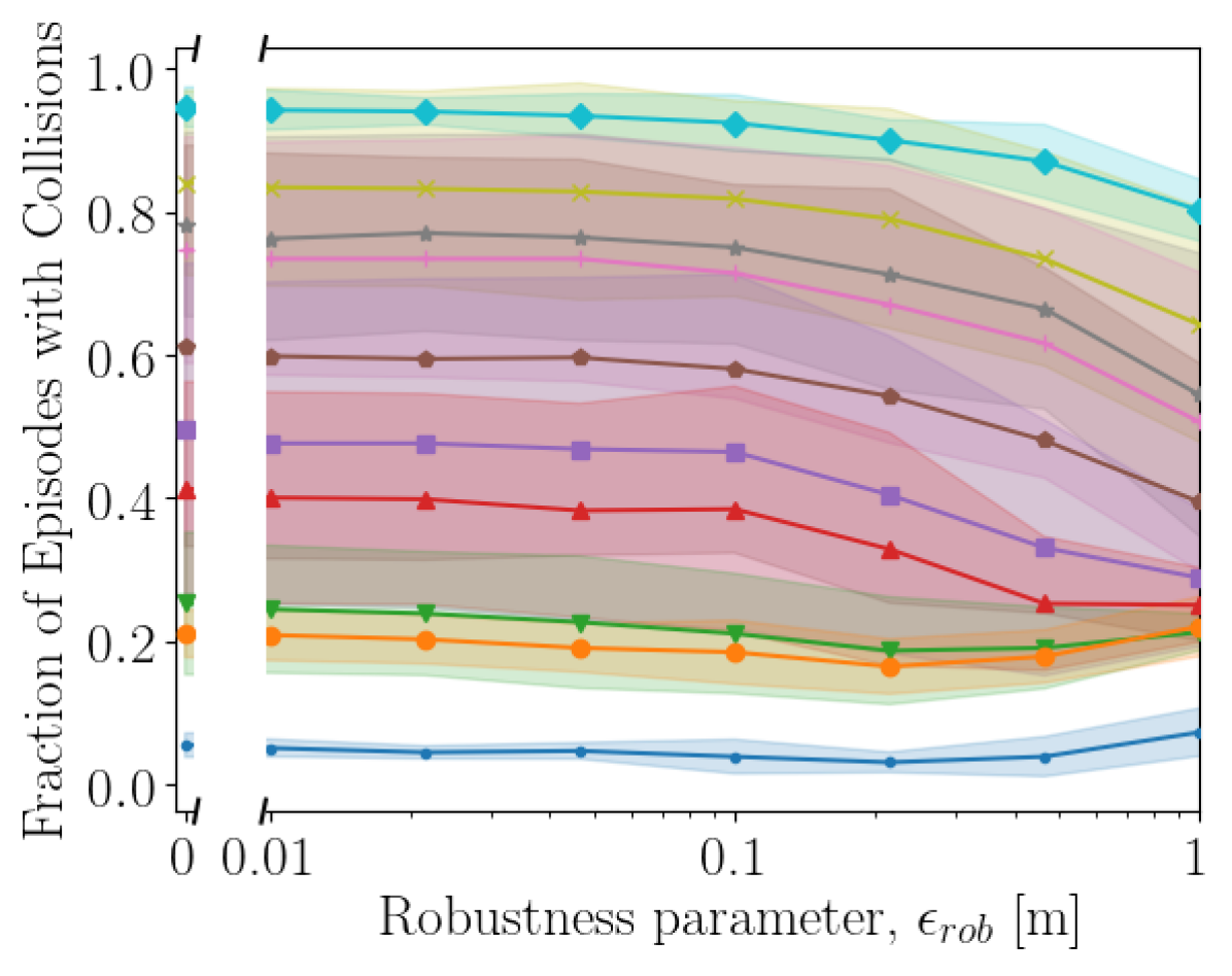
(c)

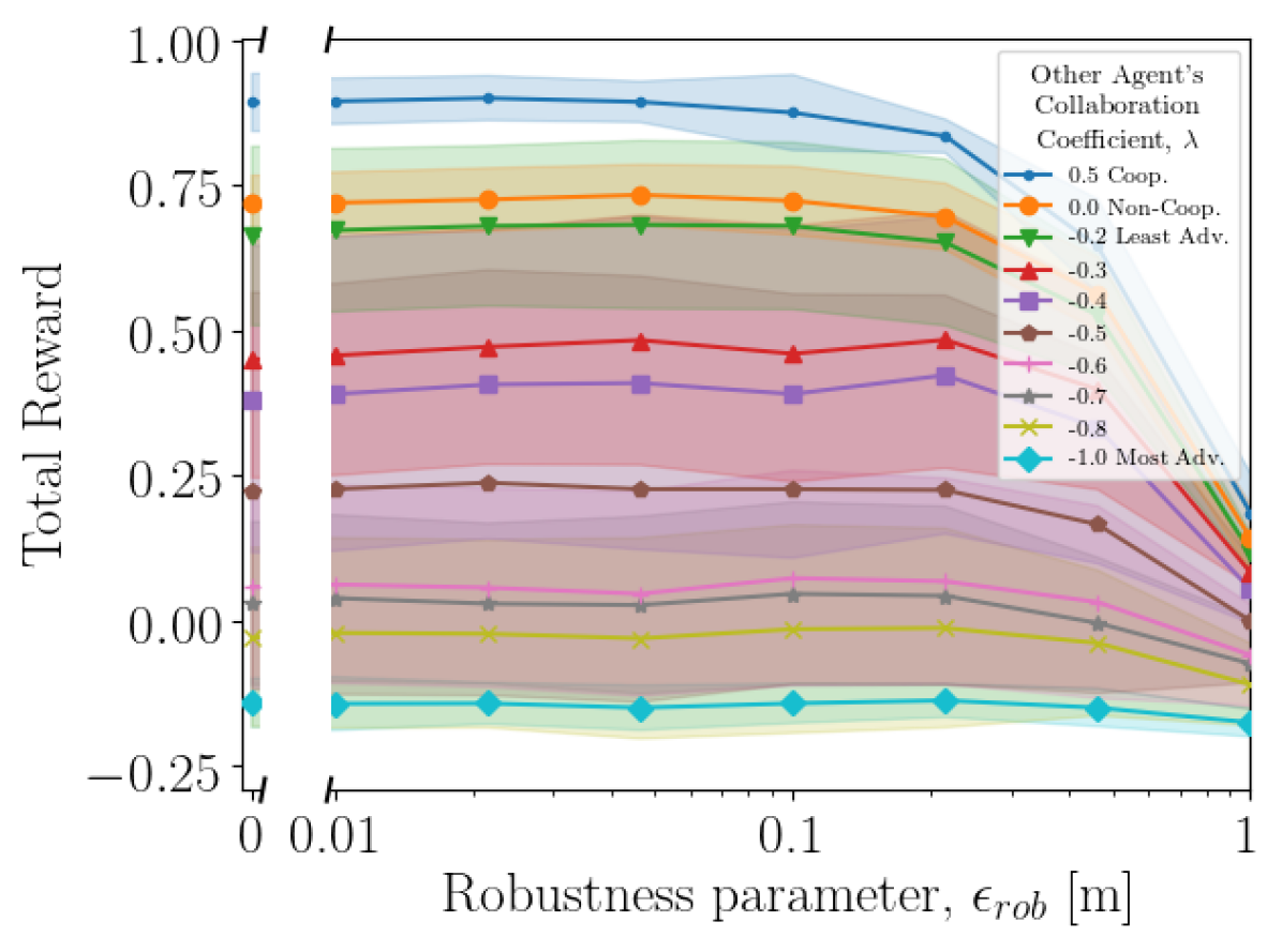
(d)

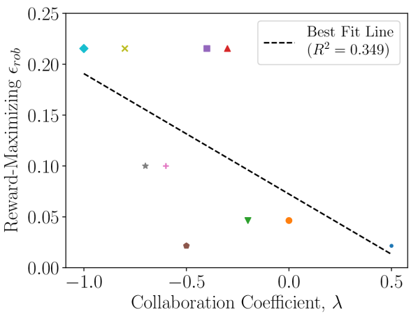
(e)

Figure 10: Robustness to Adversarial Behavior. Each curve shows a different magnitude of adversarial behavior of another agent in the collision avoidance task. The adversarially behaving other agents (negative collaboration coefficient) are able to cause many collisions with a CARRL agent trained among cooperative and non-cooperative agents. Although CARRL was not explicitly designed to handle behavioral adversaries, CARRL can reduce the number of collisions by providing robustness in the other agent’s position measurement. CARRL’s effect on reward (b) is not as strong as in Fig. 6, but the reward-maximizing ${\epsilon_{\text{rob}}>0}$ against all adversaries (c), and there is a trend of larger $\epsilon_{\text{rob}}$ working well against stronger adversaries.

In addition to observational perturbations, many real-world domains also require interaction with other agents, whose behavior could be adversarial. In the collision avoidance domain, this can be modeled by an environment agent who actively tries to collide with the CARRL agent, as opposed to the various cooperative or neutral behavior models seen in the training environment described earlier. Although the CARRL formulation does not explicitly consider behavioral adversaries, one can introduce robustness to this class of adversarial perturbation through robustness in the observation space, namely by specifying uncertainty in the other agent’s position. In other words, requiring the CARRL agent to consider worst-case positions of another agent while selecting actions causes the CARRL agent to maintain a larger spacing, which in turn prevents the adversarially behaving agent from getting close enough to cause collisions.

In the collision avoidance domain, we parameterize the adversarial “strength” by a collaboration coefficient, $\lambda$, where $\lambda=0.5$ corresponds to a nominal ORCA agent (that does half the collision avoidance), $\lambda=0$ corresponds to a non-cooperative agent that goes straight toward its goal, and $\lambda\in[-1,0)$ corresponds to an adversarially behaving agent. Adversarially behaving agents sample from a Bernoulli distribution (every 1 second) with parameter $\lvert\lambda\rvert$. If the outcome is 1, the adversarial agent chooses actions directly aiming into the CARRL agent’s projected future position, otherwise, it chooses actions moving straight toward its goal position. Thus, $\lambda=-1$ means the adversarial agent is always trying to collide with the CARRL agent.

The idea of using observational robustness to protect against behavioral uncertainty is quantified in Fig. 10, where each curve corresponds to a different behavioral adversary. Increasing the magnitude of $\lambda<0$ (increasingly strong adversaries) causes collisions with increasing frequency, since the environment transition model is increasingly different from what was seen during training. Increasing CARRL’s robustness parameter $\epsilon_{\text{rob}}$ leads to a reduction in the number of collisions, as seen in Fig. 10. Accordingly, the reward received increases for certain values of $\epsilon_{\text{rob}}>0$ (seen strongest in red, violet curves; note y-axis scale is wider than in Fig. 6). Although the impact on the reward function is not as large as in the observational uncertainty case, Fig. 10 shows that the reward-maximizing choice of $\epsilon_{\text{rob}}$ has some negative correlation the adversary’s strength (i.e., the defense should get stronger against a stronger adversary).

The same trade-off of over-conservatism for large $\epsilon_{\text{rob}}$ exists in the behavioral adversary setting. Because there are perfect observations in this experiment (just like training), CARRL has minimal effect when the other agent is cooperative (blue, ${\lambda=0.5}$). The non-cooperative curve (orange, ${\lambda=0}$) matches what was seen in Fig. 6 with $\epsilon_{\text{adv}}=0$ or $\sigma_{\text{unif}}=0$. 100 test cases with 5 seeds were used.

V-F Comparison to LP Bounds

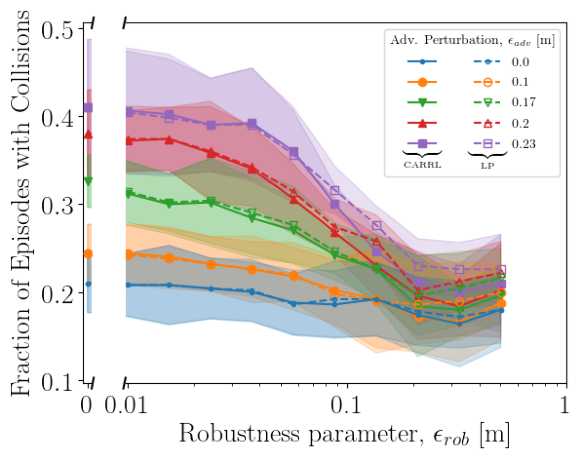
(a)

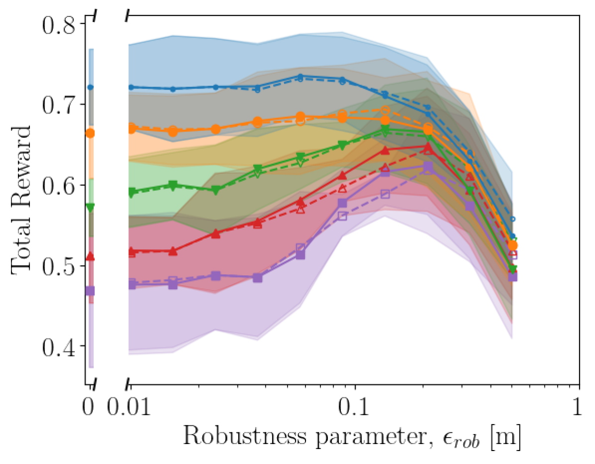
(b)

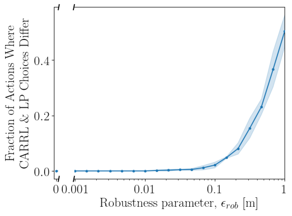
(c)

Figure 11: Greedy Convex Bounds vs. LP. Using efficient but greedy bounds on the adversarial polytope, CARRL’s action-selection produces similar performance to that of action-selection using the less relaxed LP (cf. LP-ALL in [28]) (solid vs. dashed curves in each color). In (c), CARRL and LP select identical actions on $>99\%$ of timesteps (across 60 episodes) for small $\epsilon_{\text{rob}}$, but the two methods diverge as the greedy bounds become overly conservative. Thus, for small-to-moderate $\epsilon_{\text{rob}}$, the extra computation required for the LP does not have substantial effect on decision-making.

As described in Section II, the convex relaxation approaches (e.g., Fast-Lin) provide relatively loose, but fast-to-compute bounds on DNN outputs. Equation 17 relates various bound tightnesses theoretically, which raises the question: how much better would the performance of an RL agent be, given more computation time to better approximate the worst-case outcome, $Q_{L}$?

In Fig. 11, we compare the performance of an agent following the CARRL decision rule, versus one that approximates $Q_{L}(\bm{s}_{\text{adv}},\bm{a})$ with the full (non-greedy) primal convex relaxed LP (in the collision avoidance domain with observational perturbations). Our implementation is based on the LP-ALL implementation provided in [28]. The key takeaway is that there is very little difference: the CARRL curves are solid and the LP curves are dashed, for various settings of adversarial perturbation, $\epsilon_{\text{adv}}$. The small difference in the two algorithms is explained by the fact that CARRL provides extra conservatism versus the LP (CARRL accounts for a worse worst-case than the LP), so the CARRL algorithm performs slightly better when $\epsilon_{\text{rob}}$ is set too small, and slightly worse when $\epsilon_{\text{rob}}$ is too large for the particular observational adversary.

This result is further explained by Fig. 11, where it is shown that CARRL and LP-based decision rules choose the same action ${>99\%}$ of the time for ${\epsilon<0.1}$, meaning in this experiment, the extra time spent computing the tighter bounds has little impact on the RL agent’s decisions.

V-G Intuition on Certified Bounds

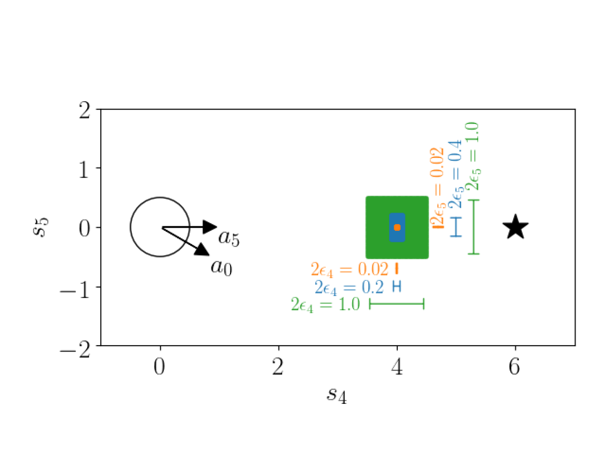
(a) Position Uncertainty of Another Agent [m]

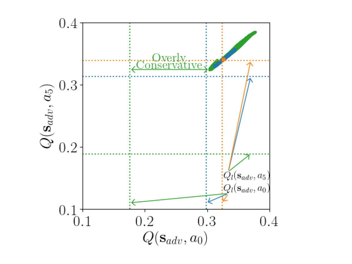
(b) Corresponding Certified Bounds & Sampled DQN Outputs

Figure 12: Influence of $\bm{\epsilon}_{\text{rob}}$ on Q-Values. In (a), the CARRL agent ($\bigcirc$) has a goal ($\bigstar$) at (6,0) and decides between two actions, $a_{0}$ and $a_{5}$. A second agent could be centered somewhere in the colored regions, corresponding to different values of $\bm{\epsilon}_{\text{rob}}$. In (b) are the corresponding Q-values for those possible states (orange, blue green regions in top-right), exhaustively sampled in each $\bm{\epsilon}_{\text{rob}}$-Ball. As $\bm{\epsilon}_{\text{rob}}$ increases, the spread of possible Q-values increases. CARRL’s lower bounds on each action, $Q_{l}(\bm{s}_{\text{adv}},a_{0})$, $Q_{l}(\bm{s}_{\text{adv}},a_{5})$, are depicted by the dotted lines. Conservatism is measured by the gap between the dashed line and the left/bottom-most sampled point. For small $\bm{\epsilon}_{\text{rob}}$ (orange), the bounds are tight; for moderate $\bm{\epsilon}_{\text{rob}}$ (blue) are moderately conservative, and for large $\bm{\epsilon}_{\text{rob}}$ (green), the linear approximation of ReLU degrades, causing excessive conservatism.

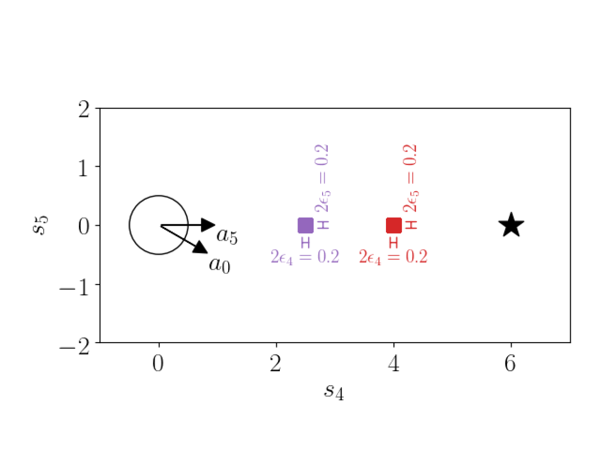
(a) Position Uncertainty of Another Agent [m]

(b) Corresponding Certified Bounds & Sampled DQN Outputs

Figure 13: Influence of $\bm{s}_{\text{adv}}$ on Q-Values. For the same $\bm{\epsilon}_{\text{rob}}$, the spread of Q-values are shown for two examples of $\bm{s}_{\text{adv}}$. When the other agent is close (purple), the Q-values are lower than when the other agent is far (red). A closer look at one of the non-convex adversarial polytopes is inset in (b). Moreover, if one instead used the heuristic of simply inflating the other agent’s radius, the Q-values would lie at the $\times$’s – in both cases, radius inflation is more conservative (further toward bottom-left) than CARRL.

Visual inspection of actual adversarial polytopes and the corresponding efficiently computed bounds provides additional intuition into the CARRL algorithm. The state uncertainty’s mapping into an adversarial polytope in the Q-value space is visualized in Figs. 13 and 13. In Fig. 13, a CARRL agent observes another agent (of the same size) positioned somewhere in the concentric, colored regions. The state uncertainty, drawn for various values of $\bm{\epsilon}_{\text{rob}}$ with $\ell_{\infty}$ norm manifests itself in Fig. 13 as a region of possible $Q(\bm{s}_{\text{adv}},a_{j})$ values, for each action, $a_{j}$. Because there are only two dimensions of state uncertainty, we can exhaustively sample $Q$-values for these states. To visualize the corresponding Q-value region in 2D, consider just two actions, $a_{0},a_{5}$ (right-most and straight actions, respectively).

The efficiently computed lower bounds, $Q_{l}$ for each action are shown as dotted lines for each of the $\bm{\epsilon}_{\text{rob}}$-Balls. Note that for small $\bm{\epsilon}_{\text{rob}}$ (orange) the bounds are quite tight to the region of possible Q-values. A larger $\bm{\epsilon}_{\text{rob}}$ region (blue) leads to looser (but still useful) bounds, and this case also demonstrates $\bm{\epsilon}_{\text{rob}}$ with non-uniform components ($\epsilon_{4}=0.1,\epsilon_{5}=0.2$, where $(4,5)$ are the indices of the other agent’s position in the state vector) For large $\bm{\epsilon}_{\text{rob}}$ (green), the bounds are very loose, as the lowest sampled Q-value for $a_{0}$ is $0.3$, but $Q_{l}(\bm{s}_{\text{adv}},a_{0})=0.16$.

This increase in conservatism with $\bm{\epsilon}_{\text{rob}}$ is explained by the formulation of Fast-Lin, in that linear bounds around an “undecided” ReLU become looser for larger input uncertainties. That is, as defined in Eq. 3, the lower linear bound of an undecided ReLU in layer $k$, neuron $i$ is $\frac{u^{(k)}_{i}\cdot l^{(k)}_{i}}{u^{(k)}_{i}+l^{(k)}_{i}}<0$ for $z^{(k)}_{i}=l^{(k)}_{i}$, whereas a ReLU can never output a negative number. This under-approximation gets more extreme for large $\epsilon_{rob,i}$, since $u^{(k)}_{i},l^{(k)}_{i}$ become further apart in the input layer, and this conservatism is propagated through the rest of the network. Per the discussion in [28], using the same slope for the upper and lower bounds has computational advantages but can lead to conservatism. The CROWN [28] algorithm generalizes this notion and allows adaptation in the slopes; connecting CROWN with CARRL is a minor change left for future work.

Moreover, expanding the possible uncertainty magnitudes without excessive conservatism and while maintaining computational efficiency could be an area of future research. Nonetheless, the lower bounds in CARRL were sufficiently tight to be beneficial across many scenarios.

In addition to $\bm{\epsilon}_{\text{rob}}$, Fig. 13 considers the impact of variations in $\bm{s}_{\text{adv}}$: when the other agent is closer to the CARRL agent (purple), the corresponding Q-values in Fig. 13 are lower for each action, than when the other agent is further away (red). Note that the shape of the adversarial polytope (region of Q-value) can be quite complicated due to the high dimensionality of the DNN (inset of Fig. 13). Furthermore, the $\times$ symbols correspond to the Q-value if the agent simply inflated the other agent’s radius to account for the whole region of uncertainty. This heuristic is highly conservative (and domain-specific), as the $\times$’s have lower Q-values than the efficiently computed lower bounds for each action in these examples.

VI Future Directions

In laying a foundation for certified adversarial robustness in deep RL, this work offers numerous future research directions in connecting deep RL algorithms and real-world, safety-critical systems.

For example, extensions of CARRL to other RL tasks will raise the question: how does the robustness analysis extend to continuous action spaces? When $\bm{\epsilon}_{\text{adv}}$ is unknown, as in our empirical results, how could $\bm{\epsilon}_{\text{rob}}$ be tuned efficiently online while maintaining robustness guarantees? How can the online robustness estimates account for uncertainties from the training process (e.g., unexplored states) in a guaranteed manner?

The key factor in the performance of robustness algorithms is the ability to precisely describe the uncertainty over which to be robust. This work provides the $\bm{\epsilon}_{\text{rob}}$, $p_{\text{rob}}$ hyperparameters to describe various shapes and sizes of uncertainties in different dimensions of the observation space and shows how this description could be applied under non-uniform, probabilistic uncertainties or a model of behavioral uncertainty. However, real-world systems also include other types of environmental uncertainties. For instance, observational uncertainties beyond $L_{p}$ balls could be studied for certifiably robust defenses in deep RL (e.g., [71, 72] in supervised learning). Moreover, how can one protect against an adversary that is allowed to plan $n$ timesteps into the future (e.g., extending [73] to model-free RL)? Are there certifiably robust defenses to uncertainties in the state transition model (e.g., disturbance forces)?

Lastly, we assume in Section IV-B that the training process has access to unperturbed observations and causes the network to converge to the optimal value function. In reality, the DQN will not exactly converge to Q*, and this additional source of uncertainty should be taken into account when computing bounds on Q. For example, a simple model of this uncertainty is to assume that training causes the DQN outputs to converge to within $\alpha$ of the true Q-values, i.e., $\lvert Q_{\text{DQN}}(\mathbf{s},\,a)-Q^{*}(\mathbf{s},\,a)\rvert\leq\alpha$. Then, the upper/lower bounds on DQN outputs can be inflated by $\alpha$ to reflect true Q-values, i.e., $Q_{L}(\mathbf{s},\,a)\leq Q_{\text{DQN}}(\mathbf{s},\,a)\leq Q_{U}(\mathbf{s},\,a)\implies Q_{L}(\mathbf{s},\,a)-\alpha\leq Q^{*}(\mathbf{s},\,a)\leq Q_{U}(\mathbf{s},\,a)+\alpha$. However, this adjustment will have no impact on the action-selection rule in Eq. 10. Moreover, ensuring convergence properties hold remains a major open problem in deep learning.

Understanding each of these areas of extension will be crucial in providing both performance and robustness guarantees for deep RL algorithms deployed on real-world systems.

VII Conclusion

This work adapted deep RL algorithms for application in safety-critical domains, by proposing an add-on certifiably robust defense to address existing failures under adversarially perturbed observations and sensor noise. The proposed extension of robustness analysis tools from the verification literature into a deep RL formulation enabled efficient calculation of a lower bound on Q-values, given the observation perturbation/uncertainty. These guaranteed lower bounds were used to efficiently solve a robust optimization formulation for action selection to provide maximum performance under worst-case observation perturbations. Moreover, the resulting policy comes with a certificate of solution quality, even though the true state and optimal action are unknown to the certifier due to the perturbations. The resulting policy (added onto trained DQN networks) was shown to improve robustness to adversaries and sensor noise, causing fewer collisions in a collision avoidance domain and higher reward in cartpole. Furthermore, the proposed algorithm was demonstrated in the presence of adversaries in the behavior space and image space, compared against a more time-intensive alternative, and visualized for particular scenarios to provide intuition on the algorithm’s conservatism.

Certified vs. Verified Terminology

Now that we have introduced our algorithm, we can more carefully describe what we mean by a certifiably robust algorithm.

First, we clarify what it means to be verified. In the context of neural network robustness, a network is verified robust for some nominal input if no perturbation within some known set can change the network’s decision from its nominal decision. A complete verification algorithm would correctly label the network as either verified robust or verified non-robust for any nominal input and perturbation set. In practice, verification algorithms often involve network relaxations, and the resulting algorithms are sound (any time the network gives an answer, the answer is true), but sometimes return that they can not verify either property.

A certificate is some piece of information that allows an algorithm to quantify its solution quality. For example, [74] uses a dual feasible point as a certificate to bound the primal solution, which allows one to compute a bound on any feasible point’s suboptimality even when the optimal value of the primal problem is unknown. When an algorithm provides a certificate, the literature commonly refers to the algorithm as certified, certifiable, or certifiably           (if it provides a certificate of          -ness).

In this work, we use a robust optimization formulation to consider worst-case possibilities on state uncertainty (Eqs. 9 and 10); this makes our algorithm robust. Furthermore, we provide a certificate on how sub-optimal the robust action recommended by our algorithm is, with respect to the optimal action at the (unknown) true state (Eq. 20). Thus, we describe our algorithm as certifiably robust or that it provides certified adversarial robustness.

As an aside, some works in computer vision/robot perception propose certifiably correct algorithms [75, 76]. In those settings, there is often a combinatorial problem that could be solved optimally with enough computation time, but practitioners prefer an algorithm that efficiently computes a (possibly sub-optimal) solution and comes with a certificate of solution quality. Our setting differs; the state uncertainty means that recovering the optimal action for the true state is not a matter of computation time. Thus, we do not aim for correctness (choosing the optimal action for the true state), but rather choose an action that maximizes worst-case performance.

Michael Everett received the S.B., S.M., and Ph.D. degrees in mechanical engineering from the Massachusetts Institute of Technology (MIT), in 2015, 2017, and 2020, respectively. He is currently a Postdoctoral Associate with the Department of Aeronautics and Astronautics at MIT. His research lies at the intersection of machine learning, robotics, and control theory, with specific interests in the theory and application of safe and robust neural feedback loops. He was an author of works that won the Best Paper Award on Cognitive Robotics at IROS 2019, the Best Student Paper Award and a Finalist for the Best Paper Award on Cognitive Robotics at IROS 2017, and a Finalist for the Best Multi-Robot Systems Paper Award at ICRA 2017. He has been interviewed live on the air by BBC Radio and his team’s robots were featured by Today Show and the Boston Globe.

Björn Lütjens is currently a Ph.D. Candidate in the Human Systems Laboratory of the Department of Aeronautics and Astronautics at MIT. He has received the S.M. degree in Aeronautics and Astronautics from MIT in 2019 and the B.Sc. degree in Engineering Science from Technical University of Munich in 2017. His research interests include deep reinforcement learning, bayesian deep learning, and climate and ocean modeling.

Jonathan P. How is the Richard C. Maclaurin Professor of Aeronautics and Astronautics at the Massachusetts Institute of Technology. He received a B.A.Sc. (aerospace) from the University of Toronto in 1987, and his S.M. and Ph.D. in Aeronautics and Astronautics from MIT in 1990 and 1993, respectively, and then studied for 1.5 years at MIT as a postdoctoral associate. Prior to joining MIT in 2000, he was an assistant professor in the Department of Aeronautics and Astronautics at Stanford University. Dr. How was the editor-in-chief of the IEEE Control Systems Magazine (2015-19) and is an associate editor for the AIAA Journal of Aerospace Information Systems and the IEEE Transactions on Neural Networks and Learning Systems. He was an area chair for International Joint Conference on Artificial Intelligence (2019) and will be the program vice-chair (tutorials) for the Conference on Decision and Control (2021). He was elected to the Board of Governors of the IEEE Control System Society (CSS) in 2019 and is a member of the IEEE CSS Technical Committee on Aerospace Control and the Technical Committee on Intelligent Control. He is the Director of the Ford-MIT Alliance and was a member of the USAF Scientific Advisory Board (SAB) from 2014-17. His research focuses on robust planning and learning under uncertainty with an emphasis on multiagent systems, and he was the planning and control lead for the MIT DARPA Urban Challenge team. His work has been recognized with multiple awards, including the 2020 AIAA Intelligent Systems Award. He is a Fellow of IEEE and AIAA.

References

- [1] B. Lütjens, M. Everett, and J. P. How, “Certified adversarial robustness for deep reinforcement learning,” in 2019 Conference on Robot Learning (CoRL), Osaka, Japan, October 2019. [Online]. Available: https://arxiv.org/pdf/1910.12908.pdf
- [2] S. Gu, E. Holly, T. Lillicrap, and S. Levine, “Deep reinforcement learning for robotic manipulation with asynchronous off-policy updates,” in 2017 IEEE International Conference on Robotics and Automation (ICRA), May 2017.
- [3] T. Fan, X. Cheng, J. Pan, P. Long, W. Liu, R. Yang, and D. Manocha, “Getting robots unfrozen and unlost in dense pedestrian crowds,” IEEE Robotics and Automation Letters, vol. 4, no. 2, pp. 1178–1185, 2019.
- [4] M. Everett, Y. F. Chen, and J. P. How, “Motion planning among dynamic, decision-making agents with deep reinforcement learning,” in IEEE/RSJ International Conference on Intelligent Robots and Systems (IROS), Sep. 2018.
- [5] C. Szegedy, W. Zaremba, I. Sutskever, J. Bruna, D. Erhan, I. Goodfellow, and R. Fergus, “Intriguing properties of neural networks,” in International Conference on Learning Representations (ICLR), 2014.
- [6] N. Akhtar and A. S. Mian, “Threat of adversarial attacks on deep learning in computer vision: A survey,” IEEE Access, vol. 6, pp. 14 410–14 430, 2018.
- [7] X. Yuan, P. He, Q. Zhu, R. R. Bhat, and X. Li, “Adversarial examples: Attacks and defenses for deep learning,” IEEE transactions on neural networks and learning systems, 2019.
- [8] A. Kurakin, I. J. Goodfellow, and S. Bengio, “Adversarial examples in the physical world,” in International Conference on Learning Representation (ICLR) (Workshop), 2017.
- [9] M. Sharif, S. Bhagavatula, L. Bauer, and M. K. Reiter, “Accessorize to a crime: Real and stealthy attacks on state-of-the-art face recognition,” in Proceedings of the 2016 ACM SIGSAC Conference on Computer and Communications Security, 2016, pp. 1528–1540.
-
[10]
Tencent Keen Security Lab, “Experimental security research of Tesla
Autopilot,” 03 2019. [Online]. Available:
https://keenlab.tencent.com/en/whitepapers/
Experimental_Security_Research_of_Tesla_Autopilot.pdf - [11] A. Mandlekar, Y. Zhu, A. Garg, L. Fei-Fei, and S. Savarese, “Adversarially robust policy learning: Active construction of physically-plausible perturbations,” in 2017 IEEE/RSJ International Conference on Intelligent Robots and Systems (IROS). IEEE, 2017, pp. 3932–3939.
- [12] A. Rajeswaran, S. Ghotra, B. Ravindran, and S. Levine, “Epopt: Learning robust neural network policies using model ensembles,” in International Conference on Learning Representations (ICLR), 2017.
- [13] F. Muratore, F. Treede, M. Gienger, and J. Peters, “Domain randomization for simulation-based policy optimization with transferability assessment,” in 2nd Annual Conference on Robot Learning, CoRL 2018, Zürich, Switzerland, 29-31 October 2018, Proceedings, 2018, pp. 700–713.
- [14] L. Pinto, J. Davidson, R. Sukthankar, and A. Gupta, “Robust adversarial reinforcement learning,” in Proceedings of the 34th International Conference on Machine Learning (ICML), ser. Proceedings of Machine Learning Research, D. Precup and Y. W. Teh, Eds., vol. 70. International Convention Centre, Sydney, Australia: PMLR, 06–11 Aug 2017, pp. 2817–2826.
- [15] J. Morimoto and K. Doya, “Robust reinforcement learning,” Neural computation, vol. 17, no. 2, pp. 335–359, 2005.
- [16] R. Ehlers, “Formal verification of piece-wise linear feed-forward neural networks,” in ATVA, 2017.
- [17] G. Katz, C. W. Barrett, D. L. Dill, K. Julian, and M. J. Kochenderfer, “Reluplex: An efficient SMT solver for verifying deep neural networks,” in Computer Aided Verification - 29th International Conference, CAV 2017, Heidelberg, Germany, July 24-28, 2017, Proceedings, Part I, 2017, pp. 97–117.
- [18] X. Huang, M. Kwiatkowska, S. Wang, and M. Wu, “Safety verification of deep neural networks,” in Computer Aided Verification, R. Majumdar and V. Kunčak, Eds. Cham: Springer International Publishing, 2017, pp. 3–29.
- [19] A. Lomuscio and L. Maganti, “An approach to reachability analysis for feed-forward relu neural networks,” CoRR, vol. abs/1706.07351, 2017. [Online]. Available: http://arxiv.org/abs/1706.07351
- [20] V. Tjeng, K. Y. Xiao, and R. Tedrake, “Evaluating robustness of neural networks with mixed integer programming,” in International Conference on Learning Representations (ICLR), 2019.
- [21] T. Gehr, M. Mirman, D. Drachsler-Cohen, P. Tsankov, S. Chaudhuri, and M. Vechev, “Ai2: Safety and robustness certification of neural networks with abstract interpretation,” in 2018 IEEE Symposium on Security and Privacy (SP), May 2018, pp. 3–18.
- [22] E. Wong and J. Z. Kolter, “Provable defenses against adversarial examples via the convex outer adversarial polytope,” in ICML, ser. Proceedings of Machine Learning Research, vol. 80, 2018, pp. 5283–5292.
- [23] S. Wang, K. Pei, J. Whitehouse, J. Yang, and S. Jana, “Efficient formal safety analysis of neural networks,” in Advances in Neural Information Processing Systems, 2018, pp. 6367–6377.
- [24] K. Dvijotham, S. Gowal, R. Stanforth, R. Arandjelovic, B. O’Donoghue, J. Uesato, and P. Kohli, “Training verified learners with learned verifiers,” arXiv preprint arXiv:1805.10265, 2018.
- [25] G. Singh, T. Gehr, M. Mirman, M. Püschel, and M. Vechev, “Fast and effective robustness certification,” in Advances in Neural Information Processing Systems, 2018, pp. 10 802–10 813.
- [26] G. Singh, T. Gehr, M. Püschel, and M. Vechev, “An abstract domain for certifying neural networks,” Proceedings of the ACM on Programming Languages, vol. 3, no. POPL, pp. 1–30, 2019.
- [27] T. Weng, H. Zhang, H. Chen, Z. Song, C. Hsieh, L. Daniel, D. Boning, and I. Dhillon, “Towards fast computation of certified robustness for relu networks,” in International Conference on Machine Learning (ICML), 2018.
- [28] H. Zhang, T.-W. Weng, P.-Y. Chen, C.-J. Hsieh, and L. Daniel, “Efficient neural network robustness certification with general activation functions,” in Advances in Neural Information Processing Systems 31, S. Bengio, H. Wallach, H. Larochelle, K. Grauman, N. Cesa-Bianchi, and R. Garnett, Eds. Curran Associates, Inc., 2018, pp. 4939–4948.
- [29] H. Salman, G. Yang, H. Zhang, C.-J. Hsieh, and P. Zhang, “A convex relaxation barrier to tight robustness verification of neural networks,” in Advances in Neural Information Processing Systems, 2019, pp. 9832–9842.
- [30] I. Ilahi, M. Usama, J. Qadir, M. U. Janjua, A. Al-Fuqaha, D. T. Hoang, and D. Niyato, “Challenges and countermeasures for adversarial attacks on deep reinforcement learning,” arXiv preprint arXiv:2001.09684, 2020.
- [31] I. Goodfellow, J. Shlens, and C. Szegedy, “Explaining and harnessing adversarial examples,” in International Conference on Learning Representations (ICLR), 2015.
- [32] S. Huang, N. Papernot, I. Goodfellow, Y. Duan, and P. Abbeel, “Adversarial attacks on neural network policies,” 2017.
- [33] V. Behzadan and A. Munir, “Vulnerability of deep reinforcement learning to policy induction attacks,” in International Conference on Machine Learning and Data Mining in Pattern Recognition (MLDM). Springer, 2017, pp. 262–275.
- [34] C.-H. H. Yang, J. Qi, P.-Y. Chen, Y. Ouyang, I.-T. D. Hung, C.-H. Lee, and X. Ma, “Enhanced adversarial strategically-timed attacks against deep reinforcement learning,” in ICASSP 2020-2020 IEEE International Conference on Acoustics, Speech and Signal Processing (ICASSP). IEEE, 2020, pp. 3407–3411.
- [35] W. Uther and M. Veloso, “Adversarial reinforcement learning,” In Proceedings of the AAAI Fall Symposium on Model Directed Autonomous Systems, Tech. Rep., 1997.
- [36] A. Gleave, M. Dennis, N. Kant, C. Wild, S. Levine, and S. Russell, “Adversarial policies: Attacking deep reinforcement learning,” 2020.
- [37] M. L. Littman, “Markov games as a framework for multi-agent reinforcement learning,” in Machine learning proceedings 1994. Elsevier, 1994, pp. 157–163.
- [38] A. Kurakin, I. J. Goodfellow, and S. Bengio, “Adversarial machine learning at scale,” in International Conference on Learning Representations (ICLR), 2017.
- [39] A. Madry, A. Makelov, L. Schmidt, D. Tsipras, and A. Vladu, “Towards deep learning models resistant to adversarial attacks,” in International Conference on Learning Representations (ICLR), 2018.
- [40] J. Kos and D. Song, “Delving into adversarial attacks on deep policies,” in International Conference on Learning Representations (ICLR) (Workshop), 2017.
- [41] M. Mirman, M. Fischer, and M. Vechev, “Distilled agent DQN for provable adversarial robustness,” 2019. [Online]. Available: https://openreview.net/forum?id=ryeAy3AqYm
- [42] N. Papernot, P. McDaniel, X. Wu, S. Jha, and A. Swami, “Distillation as a defense to adversarial perturbations against deep neural networks,” in 2016 IEEE Symposium on Security and Privacy (SP), May 2016, pp. 582–597.
- [43] F. Tramèr, A. Kurakin, N. Papernot, I. Goodfellow, D. Boneh, and P. McDaniel, “Ensemble adversarial training: Attacks and defenses,” in International Conference on Learning Representations (ICLR), 2018.
- [44] W. Xu, D. Evans, and Y. Qi, “Feature squeezing: Detecting adversarial examples in deep neural networks,” in Network and Distributed Systems Security Symposium (NDSS). The Internet Society, 2018.
- [45] N. Carlini and D. Wagner, “Adversarial examples are not easily detected: Bypassing ten detection methods,” in Proceedings of the 10th ACM Workshop on Artificial Intelligence and Security, ser. AISec ’17. New York, NY, USA: ACM, 2017, pp. 3–14.
- [46] W. He, J. Wei, X. Chen, N. Carlini, and D. Song, “Adversarial example defenses: Ensembles of weak defenses are not strong,” in Proceedings of the 11th USENIX Conference on Offensive Technologies, ser. WOOT’17. Berkeley, CA, USA: USENIX Association, 2017, pp. 15–15.
- [47] A. Athalye, N. Carlini, and D. Wagner, “Obfuscated gradients give a false sense of security: Circumventing defenses to adversarial examples,” in Proceedings of the 35th International Conference on Machine Learning (ICML), ser. Proceedings of Machine Learning Research, J. Dy and A. Krause, Eds., vol. 80. Stockholmsmässan, Stockholm Sweden: PMLR, 10–15 Jul 2018, pp. 274–283.
- [48] J. Uesato, B. O’Donoghue, P. Kohli, and A. van den Oord, “Adversarial risk and the dangers of evaluating against weak attacks,” in Proceedings of the 35th International Conference on Machine Learning (ICML), ser. Proceedings of Machine Learning Research, J. Dy and A. Krause, Eds., vol. 80. Stockholmsmässan, Stockholm Sweden: PMLR, 10–15 Jul 2018, pp. 5025–5034.
- [49] J. García and F. Fernández, “A comprehensive survey on safe reinforcement learning,” Journal of Machine Learning Research, vol. 16, pp. 1437–1480, 2015.
- [50] M. Heger, “Consideration of risk in reinforcement learning,” in Machine Learning Proceedings 1994, W. W. Cohen and H. Hirsh, Eds. San Francisco (CA): Morgan Kaufmann, 1994, pp. 105 – 111.
- [51] A. Tamar, “Risk-sensitive and efficient reinforcement learning algorithms,” Ph.D. dissertation, Technion - Israel Institute of Technology, Faculty of Electrical Engineering, 2015.
- [52] P. Geibel, “Risk-sensitive approaches for reinforcement learning,” Ph.D. dissertation, University of Osnabrück, 2006.
- [53] J. M. Cohen, E. Rosenfeld, and J. Z. Kolter, “Certified adversarial robustness via randomized smoothing,” arXiv preprint arXiv:1902.02918, 2019.
- [54] V. Mnih, K. Kavukcuoglu, D. Silver, A. A. Rusu, J. Veness, M. G. Bellemare, A. Graves, M. Riedmiller, A. K. Fidjeland, G. Ostrovski, S. Petersen, C. Beattie, A. Sadik, I. Antonoglou, H. King, D. Kumaran, D. Wierstra, S. Legg, and D. Hassabis, “Human-level control through deep reinforcement learning,” in Nature. Nature Publishing Group, a division of Macmillan Publishers Limited., 2015, vol. 518.
- [55] V. Mnih, A. P. Badia, M. Mirza, A. Graves, T. Lillicrap, T. Harley, D. Silver, and K. Kavukcuoglu, “Asynchronous methods for deep reinforcement learning,” in International conference on machine learning, 2016, pp. 1928–1937.
- [56] J. Schulman, F. Wolski, P. Dhariwal, A. Radford, and O. Klimov, “Proximal policy optimization algorithms,” arXiv preprint arXiv:1707.06347, 2017.
- [57] T. Haarnoja, A. Zhou, P. Abbeel, and S. Levine, “Soft actor-critic: Off-policy maximum entropy deep reinforcement learning with a stochastic actor,” arXiv preprint arXiv:1801.01290, 2018.
- [58] P. Christodoulou, “Soft actor-critic for discrete action settings,” arXiv preprint arXiv:1910.07207, 2019.
- [59] M. Babaeizadeh, I. Frosio, S. Tyree, J. Clemons, and J. Kautz, “Ga3c: Gpu-based a3c for deep reinforcement learning,” CoRR abs/1611.06256, 2016.
- [60] P.-Y. Chen, H. Zhang, Y. Sharma, J. Yi, and C.-J. Hsieh, “Zoo: Zeroth order optimization based black-box attacks to deep neural networks without training substitute models,” in Proceedings of the 10th ACM Workshop on Artificial Intelligence and Security, 2017, pp. 15–26.
- [61] M. Everett and J. How, “Gym: Collision avoidance,” 2020. [Online]. Available: https://github.com/mit-acl/gym-collision-avoidance
- [62] G. Brockman, V. Cheung, L. Pettersson, J. Schneider, J. Schulman, J. Tang, and W. Zaremba, “Openai gym,” 2016.
- [63] J. P. van den Berg, S. J. Guy, M. C. Lin, and D. Manocha, “Reciprocal n-body collision avoidance,” in International Symposium on Robotics Research (ISRR), 2009.
- [64] J. Snoek, H. Larochelle, and R. P. Adams, “Practical bayesian optimization of machine learning algorithms,” in Advances in Neural Information Processing Systems (NeurIPS) 25, F. Pereira, C. J. C. Burges, L. Bottou, and K. Q. Weinberger, Eds. Curran Associates, Inc., 2012, pp. 2951–2959.
- [65] A. G. Barto, R. S. Sutton, and C. W. Anderson, “Neuronlike adaptive elements that can solve difficult learning control problems,” IEEE transactions on systems, man, and cybernetics, no. 5, pp. 834–846, 1983.
- [66] A. Hill, A. Raffin, M. Ernestus, A. Gleave, A. Kanervisto, R. Traore, P. Dhariwal, C. Hesse, O. Klimov, A. Nichol, M. Plappert, A. Radford, J. Schulman, S. Sidor, and Y. Wu, “Stable baselines,” 2018. [Online]. Available: https://github.com/hill-a/stable-baselines
- [67] M. G. Bellemare, Y. Naddaf, J. Veness, and M. Bowling, “The arcade learning environment: An evaluation platform for general agents,” Journal of Artificial Intelligence Research, vol. 47, pp. 253–279, jun 2013.
- [68] B. W. Mott, T. Team et al., “Stella: a multiplatform atari 2600 vcs emulator,” 1995.
- [69] A. Raffin, “Rl baselines zoo,” https://github.com/araffin/rl-baselines-zoo, 2018.
- [70] H. Zhang, H. Chen, C. Xiao, S. Gowal, R. Stanforth, B. Li, D. Boning, and C.-J. Hsieh, “Crown-ibp: Towards stable and efficient training of verifiably robust neural networks,” 2020. [Online]. Available: https://github.com/huanzhang12/CROWN-IBP
- [71] T. Brown, D. Mané, A. Roy, M. Abadi, and J. Gilmer, “Adversarial patch,” Conference on Neural Information Processing Systems (NeurIPS) Workshop, 2017.
- [72] E. Wong, F. R. Schmidt, and J. Z. Kolter, “Wasserstein adversarial examples via projected sinkhorn iterations,” vol. 97, 2019.
- [73] Y.-S. Wang, T.-W. Weng, and L. Daniel, “Verification of neural network control policy under persistent adversarial perturbation,” NeurIPS Workshop on Safety and Robustness in Decision Making, 2019.
- [74] S. Boyd and L. Vandenberghe, Convex optimization. Cambridge university press, 2004.
- [75] A. S. Bandeira, “A note on probably certifiably correct algorithms,” Comptes Rendus Mathematique, vol. 354, no. 3, pp. 329–333, 2016.
- [76] H. Yang, J. Shi, and L. Carlone, “Teaser: Fast and certifiable point cloud registration,” 2020. [Online]. Available: https://github.com/MIT-SPARK/TEASER-plusplus