Cosmological Constraints on Scalar Field Dark Matter

Abstract

This paper aims to put constraints on the parameters of the Scalar Field Dark Matter (SFDM) model, when dark matter is described by a free real scalar field filling the whole Universe, plus a cosmological constant term. By using a compilation of 51 $H(z)$ data and 1048 Supernovae data from Panteon, a lower limit for the mass of the scalar field was obtained, $m\geq 5.1\times 10^{-34}$eV and $H_{0}=69.5^{+2.0}_{-2.1}\text{ km s}^{-1}\text{Mpc}^{-1}$. Also, the present dark matter density parameter was obtained as $\Omega_{\phi}=0.230^{+0.033}_{-0.031}$ at $2\sigma$ confidence level. The results are in good agreement to standard model of cosmology, showing that SFDM model is viable in describing the dark matter content of the universe.

I Introduction

Astronomical observations provide us with important informations about the evolution of the universe. The type Ia Supernovae (SNe Ia) data endow us with strong evidences of the current accelerated expansion of the universe due to dark energy (DE) and the spectrum of Cosmic Microwave Background (CMB) radiation states that the large-scale universe is homogeneous and isotropic at least for anisotropies up to order of $10^{-5}$. Using the Friedmann-Robertson-Walker metric (FRW) and the General Relativity equations, we obtain the standard cosmological model, named $\Lambda$CDM model, which describes an universe nearly spatially flat and currently undergoing an accelerating phase due to recent domination of a component with negative pressure represented by $\Lambda$. This component represents DE, which corresponds to about $70\%$ of the energy content of the Universe, while Cold Dark Matter (CDM) in the halo of galaxies represents $25\%$ and the ordinary baryonic matter corresponds to about $5\%$. Currently, the contribution of radiation is negligible.

This is the model that, in general, satisfactorily describes observational data, however it presents some problems due to misunderstanding of the nature of DM p8 ; pp and DE W1 ; W2 . This stimulates the search for new models describing these unknown components.

Bosonic scalar fields are important objects of study in several branches of theoretical physics, with applications from Quantum Field Theory to Cosmology. They are present since the origin of the Universe, for instance the fundamental scalar fields describing the grand unified theory (GUT) GL ; LCF and, soon after, in the evolution of the universe, being responsible for inflation and reheating mechanisms GA ; LA . In addition, some authors have also assumed the nature of DM and DE as essentially represented by scalar fields me1 ; me2 ; me3 ; me4 ; me5 . Although only the Higgs boson and some mesons have been detected experimentally in nature as true scalar fields, other scalar fields could be present in the universe, as predicted by supersymmetric models.

Scalar Field Dark Matter models, which treats the DM as formed by a real scalar field $\phi$ minimally coupled to gravity subject to a potential $V(\phi)$, have provided interesting results recently 1 ; 2 ; js ; 3 . In 1 ; 2 it has been proposed that DM is an ultralight zero spin boson with a Compton wavelength of the order of few kpc, condensing at high temperatures of the order of $\sim$ TeV, leading to formation of Bose-Einstein condensates in the early universe. Thus, droplets of DM were formed, which would become the halos of galaxies hg . This implies all galaxies to be very similar, having their halos formed practically at the same time at high redshift. The DM scalar field mass estimated was of about $10^{-22}$ eV. A more recent work t1 has found an inferior limit for the SFDM mass of the order of $10^{-32}$ eV, a value close to the lower limit found in js of $m>10^{-33}$ eV, using combination of SNe Ia s1 and $H(z)$ h1 data.

In this work we study the recent evolution of the universe driven by a SFDM model in which the DM particle is represented by a real, massive and homogeneous scalar field $\phi$, which is minimally coupled to gravity. In section II, we begin by introducing the dynamic equations of the SFDM model. In section III, we develop an approximation in order to obtain more efficient numerical solutions for the field. In section IV, the observational data used is briefly described. In section V, the model is analysed according to Bayesian Statistics b1 ; b2 , using the Monte Carlo Markov Chain (MCMC) method M1 ; M2 ; M3 ; M4 as a tool. Finally, in section VI, we present the conclusions.

II Dynamics of SFDM

The dynamic equations of the SFDM model plus baryonic ordinary matter and a cosmological constant $\Lambda$ term are, in a spatially flat FRW background js :

$$\dot{H} =-\frac{\kappa^{2}}{2}\left(\dot{\phi}^{2}+\rho_{b}\right),$$ (1)

$$\ddot{\phi}+3H\dot{\phi}+\frac{dV}{d\phi} =0,$$ (2)

$${\dot{\rho}_{b}}+3H\rho_{b} =0,$$ (3)

$${\dot{\rho}_{\Lambda}} =0,$$ (4)

together with Friedmann constraint:

$$H^{2}=\frac{\kappa^{2}}{3}\left(\rho_{\phi}+\rho_{b}+\rho_{\Lambda}\right)\,,$$ (5)

where $\rho_{b}$, $\rho_{\phi}$ and $\rho_{\Lambda}$ correspond to the energy densities of baryonic matter, scalar field and cosmological constant term, with $\kappa^{2}\equiv 8\pi G$ and $H\equiv\dot{a}/a$ the Hubble parameter.

Using a quadratic potential of the form $V(\phi)=m^{2}\phi^{2}/2$, where $m$ is the physical mass of the scalar field, and using the change of variables js ,

$$r\cos\theta\equiv\frac{\kappa}{\sqrt{6}}\frac{\dot{\phi}}{H},\,\,\,r\sin\theta\equiv\frac{\kappa}{\sqrt{6}}\frac{m\phi}{H},\,\,\,\theta\equiv\tan^{-1}\frac{m\phi}{\dot{\phi}},\,\,\,b\equiv\frac{\kappa}{\sqrt{3}}\frac{\sqrt{\rho_{b}}}{H},\,\,\,l\equiv\frac{\kappa}{\sqrt{3}}\frac{\sqrt{\rho_{\Lambda}}}{H},$$ (6)

we can rewrite the dynamic equations of the model, (1)-(4), as:

$$r^{\prime} =-3r\cos^{2}(\theta)+\frac{3}{2}\Pi r,$$ (7)

$$\theta^{\prime} =s+\frac{3}{2}\sin(2\theta),$$ (8)

$$b^{\prime} =\frac{3}{2}\left(\Pi-1\right)\,b,$$ (9)

$$l^{\prime} =\frac{3}{2}\Pi l,$$ (10)

$$s^{\prime} ={3\over 2}\Pi s.$$ (11)

where $\Pi=2r^{2}\cos^{2}(\theta)+b^{2}$ and $s$ is a new parameter, defined by $s\equiv m/H$. A prime denotes derivative with respect to $N\equiv\ln a$, the “e-folding number”.

Finally, we complete the new system of equations, (7)-(11), with a sixth equation that allows us to analyse SNe Ia data, which depends on the luminosity distance $D_{L}$ given in terms of the comoving distance, $D_{C}$:

$$D_{L}=(1+z)\frac{H_{0}}{c}D_{C}\,,$$ (12)

where $c$ is the speed of light. Since $D_{C}$ depends on $H(z)$ but we do not have an analytic expression for $H(z)$, we need a differential equation for $D_{C}$. For a spatially flat universe we can write:

$$\frac{dD_{C}}{dz}\equiv\frac{1}{E(z)},$$ (13)

with $E(z)\equiv\frac{H(z)}{H_{0}}=\frac{\mu}{s}$ and $\mu=m/H_{0}$. Regarding the independent variable $N$, we have:

$$D^{\prime}(N)=-\frac{e^{-N}s}{\mu}\,,$$ (14)

which corresponds to the sixth equation for the dynamic system (7)-(11). The initial conditions at $N=0$ (today) are given by the vector of parameters $\vec{r}_{0}$:

$$\vec{r}_{0}=\left(\sqrt{\Omega_{\phi 0}},\theta_{0},\sqrt{\Omega_{b0}},\sqrt{1-\Omega_{\phi 0}-\Omega_{b0}},\mu\right)\,.$$ (15)

As well known js , this leads to a high oscillatory behaviour of the field, a behaviour which corresponds to an average equation of state (EOS) corresponding to dust, $\langle\omega\rangle\approx 0$. In order to make the numerical solution of the system (6) more efficient, next we seek for an approximation in the mass interval that we are interested, namely, $m\gg H_{0}$ ($\mu\gg 1$).

III JWKB approximation

Assuming a time dependent $\eta$ function, $\eta(t)$, we can write the scalar field dynamic equation (2) as:

$$\phi^{\prime\prime}(\eta)+\phi^{\prime}(\eta)\left(\frac{\ddot{\eta}+3H\dot{\eta}}{\dot{\eta}^{2}}\right)+\frac{m^{2}\phi}{\dot{\eta}^{2}} = 0\,,$$ (16)

where we use $\phi^{\prime}(\eta)\equiv\frac{d\phi}{d\eta}$. In order to use the JWKB approximation we must eliminate the term $\phi^{\prime}(\eta)$, so we must cancel the term in parentheses of the above relation. This term vanishes when

$$\ddot{\eta}+3H\dot{\eta}=0,$$

whose solution is

$$\dot{\eta}=Ca^{-3}.$$ (17)

where $C$ is a constant. Thus, equation (16) becomes:

$$\phi^{\prime\prime}(\eta)+\frac{m^{2}a^{6}\phi}{C^{2}}=0\,.$$ (18)

The above equation is of the form,

$$\frac{d^{2}y(x)}{dx^{2}}+h^{2}\psi(x)y(x)=0\,,$$ (19)

with $h=m/C$ a constant. The approximate solution is given by Jeffreys25 ; Ratra91 :

$$y(x) = \psi(x)^{-\frac{1}{4}}(A\cos{L}+B\sin{L})\,,$$ (20)

$$L = \int_{0}^{x}\psi(x)^{\frac{1}{2}}dx\,,$$ (21)

with $A$ and $B$ constants. This allows us to write a solution for $\phi$:

$$\phi = a^{-\frac{3}{2}}\left(\frac{m}{C}\right)^{-\frac{1}{2}}\left[A\cos{\left(\int\frac{ma^{3}}{C}d\eta\right)}+B\sin{\left(\int\frac{ma^{3}}{C}d\eta\right)}\right]\,,$$ (22)

$$= a^{-\frac{3}{2}}\left(\frac{m}{C}\right)^{-\frac{1}{2}}\left[A\cos{\left(\int mdt\right)}+B\sin{\left(\int mdt\right)}\right]\,,$$ (23)

$$\phi = a^{-\frac{3}{2}}\left[\bar{A}\cos{\left(mt\right)}+\bar{B}\sin{\left(mt\right)}\right]\,.$$ (24)

Redefining constants as

$$\bar{A} = \alpha\sin{\beta}\,,$$

$$\bar{B} = \alpha\cos{\beta}\,,$$

using the relation $\mu=\frac{m}{H_{0}}$ and defining $\tau=H_{0}t$, we can rewrite the equation (24) as a function of $N$ and $\tau$:

$$\phi = \alpha e^{-\frac{3N}{2}}\sin{(\mu\tau+\beta)}\,.$$ (25)

Finally, we can write a dimensionless quantity $\Phi$,

$$\Phi\equiv\sqrt{\frac{8\pi G}{3}}\phi\,,$$ (26)

which will give a solution

$$\Phi(N) = \alpha e^{-\frac{3N}{2}}\sin{(\mu\tau+\beta)}\,.$$ (27)

where we have defined $\alpha^{\prime}\equiv\sqrt{\frac{8\pi G}{3}}\alpha$ and then we have dropped the prime on $\alpha^{\prime}$. It allows us to rewrite the dynamic variables $r$ and $\theta$ as

$$r = \sqrt{\Omega_{\phi}}=\sqrt{\frac{1}{H^{2}}\left[\frac{H_{0}^{2}}{2}\left(\frac{d\Phi}{d\tau}\right)^{2}+\frac{m^{2}\Phi^{2}}{2}\right]}\,,$$ (28)

$$\theta = \tan^{-1}{\frac{\mu\Phi}{{d\Phi/d\tau}}}\,,$$ (29)

with $\frac{d}{dt}=H_{0}\frac{d}{d\tau}\,$.

The initial conditions are given in $\tau=0$,

$$\Omega_{\phi 0} =\alpha^{2}\left[\frac{9\sin^{2}{\beta}}{8}-\frac{3\mu\sin{2\beta}}{4}+\frac{\mu^{2}}{2}\right]\,,$$ (30)

$$\theta_{0} =\tan^{-1}{\frac{\mu\sin{\beta}}{{\mu\cos{\beta}-\frac{3}{2}\sin{\beta}}}}\,,$$ (31)

from which we can write $\alpha$ as a function of $\beta$:

$$\alpha=\sqrt{\frac{8\Omega_{\phi 0}}{9\sin^{2}{\beta}-6\mu\sin{2\beta}+4\mu^{2}}}\,.$$ (32)

It is important to mention that the denominator in (32) is always positive for any $\beta$ and for $\mu\neq 0$. Using relation (26), the Friedmann equation becomes js :

$$\left(\frac{H}{H_{0}}\right)^{2}=\frac{\frac{1}{2}\mu^{2}\Phi(N)^{2}+\Omega_{b0}e^{-3N}+\Omega_{\Lambda 0}}{1-\frac{1}{2}\Phi^{\prime}(N)^{2}}\,,$$ (33)

which allows us to find a relation for $\frac{dN}{d\tau}=\frac{H}{H_{0}}$:

$$\frac{dN}{d\tau}=\frac{\sqrt{\Delta}-3\mu\alpha^{2}\sin\left[2(\beta+\mu\tau)\right]}{8e^{3N}-9\alpha^{2}\sin^{2}(\beta+\mu\tau)}$$ (34)

where

$$\Delta\equiv\left[8e^{3N}-9\alpha^{2}\sin^{2}(\beta+\mu\tau)\right]\left[8\left(\Omega_{b}+\Omega_{\Lambda}e^{3N}\right)+4\mu^{2}\alpha^{2}\sin^{2}(\beta+\mu\tau)\right]+32\mu^{2}\alpha^{2}e^{3N}\cos^{2}(\beta+\mu\tau)$$ (35)

Defining $\gamma\equiv\frac{1}{\mu}$, we can expand (34) in series around $\gamma=0$ ($\mu\rightarrow\infty$), obtaining to the first order:

$$\frac{dN}{d\tau}\simeq E_{\Lambda}-\frac{3\gamma}{4}e^{-3N}\Omega_{\phi}\left\{\sin\left[2\left(\beta+\frac{\tau}{\gamma}\right)\right]-e^{\frac{3N}{2}}\sin{\left(2\beta\right)}\right\}\,,$$ (36)

where $E_{\Lambda}=\sqrt{(\Omega_{b}+\Omega_{\phi})e^{-3N}+\Omega_{\Lambda}}$ and the second term corresponds to a first order correction. From this result we can see that the $\Lambda$CDM background behaviour is a limit for SFDM when $m\rightarrow\infty$. In order to solve it numerically we consider $\tau=\tau_{\Lambda}$, where $\tau_{\Lambda}$ is the age in $\Lambda$CDM model. That is, as $\tau$ only appears in the first order term, replacing it by the zeroth order approximation, keeps it correct at first order on $\gamma$.

IV Samples

IV.1 $H(z)$ dataset

In order to constrain the free parameters, we use the Hubble parameter ($H(z)$) data in different redshift values. These kind of observational data are quite reliable because in general such observational data are independent of the background cosmological model, just relying on astrophysical assumptions. We have used the currently most complete compilation of $H(z)$ data, with 51 measurements MaganaEtAl18 .

At the present time, the most important methods for obtaining $H(z)$ data are (i) through “cosmic chronometers”, for example, the differential age of galaxies (DAG) Simon et al. (2005); Stern et al. (2010); Moresco et al. (2012); Zhang et al. (2012); Moresco (2015); Moresco et al. (2016), (ii) measurements of peaks of baryonic acoustic oscillations (BAO) Gaztañaga et al. (2009); Blake et al. (2012); Busca et al. (2012); Anderson et al. (2013); Font-Ribeira et al. (2013); Delubac et al. (2014) and (iii) through correlation function of luminous red galaxies (LRG) Chuang & Wang (2013); Oka et al. (2014).

Among these methods for estimating $H(z)$, the 51 data compilation as grouped by MaganaEtAl18 , consists of 20 clustering (BAO+LRG) and 31 differential age $H(z)$ data.

Differently from MaganaEtAl18 , we choose not to use $H_{0}$ in our main results here, due to the current tension among $H_{0}$ values estimated from different observations (RiessEtAl16, ; Planck16, ; BernalEtAl16, ).

IV.2 SNe Ia

We have chosen to work with one of the largest SNe Ia sample to date, namely, the Pantheon sample pantheon . This sample consists of 279 SNe Ia from Pan-STARRS1 (PS1) Medium Deep Survey ($0.03<z<0.68$), combined with distance estimates of SNe Ia from Sloan Digital Sky Survey (SDSS), SNLS and various low-$z$ and Hubble Space Telescope samples to form the largest combined sample of SNe Ia, consisting of a total of 1048 SNe Ia in the range of $0.01<z<2.3$.

As explained on pantheon , the PS1 light-curve fitting has been made with SALT2 GuyEtAl10 , as it has been trained on the JLA sample BetouleEtAl14 . Three quantities are determined in the light-curve fit that are needed to derive a distance: the colour $c$, the light-curve shape parameter $x_{1}$ and the log of the overall flux normalization $m_{B}$.

The SALT2 light-curve fit parameters are transformed into distances using a modified version of the Tripp formula Tripp98 ,

$$\mu=m_{B}-M+\alpha x_{1}-\beta c+\Delta_{M}+\Delta_{B},$$ (37)

where $\mu$ is the distance modulus, $\Delta_{M}$ is a distance correction term based on the host galaxy mass of the SN, and $\Delta_{B}$ is a distance correction factor based on predicted biases from simulations. As can be seen, $\alpha$ is the coefficient of the relation between luminosity and stretch, while $\beta$ is the coefficient of the relation between luminosity and color, and $M$ is the absolute $B$-band magnitude of a fiducial SN Ia with $x_{1}=0$ and $c=0$.

Differently from previous SNe Ia samples, like JLA BetouleEtAl14 , Pantheon uses a calibration method named BEAMS with Bias Corrections (BBC), which allows to determine SNe Ia distances without one having to fit SNe parameters jointly with cosmological parameters. Thus, Pantheon provide directly corrected $m_{B}$ estimates in order to constrain cosmological parameters alone.

The systematic uncertainties were propagated through a systematic uncertainty matrix. An uncertainty matrix C was defined such that

$$\mathbf{C}=\mathbf{D}_{\mathrm{stat}}+\mathbf{C}_{\mathrm{sys}}.$$ (38)

The statistical matrix $\mathbf{D}_{\mathrm{stat}}$ has only diagonal components that includes photometric errors of the SN distance, the distance uncertainty from the mass step correction, the uncertainty from the distance bias correction, the uncertainty from the peculiar velocity uncertainty and redshift measurement uncertainty in quadrature, the uncertainty from stochastic gravitational lensing, and the intrinsic scatter.

V Analyses and Results

In our analyses, we have chosen flat priors for all parameters, so always the posterior distributions are proportional to the likelihoods.

For $H(z)$ data, the likelihood distribution function is given by $\mathscr{L}_{H}\propto e^{-\frac{\chi^{2}_{H}}{2}}$, where

$$\chi^{2}_{H}=\sum_{i=1}^{51}\frac{{\left[H_{obs,i}-H(z_{i},\mathbf{s})\right]}^{2}}{\sigma^{2}_{H_{i},obs}},$$ (39)

The $\chi^{2}$ function for Pantheon is given by

$$\chi^{2}=\mathbf{\Delta m}^{T}\cdot\mathbf{C}^{-1}\cdot\mathbf{\Delta m},$$ (40)

where C is the same from (38), $\mathbf{\Delta m}=m_{B}-m_{\mathrm{mod}}$, and

$$m_{\mathrm{mod}}=5\log_{10}D_{L}(z)+\mathcal{M},$$ (41)

where $\mathcal{M}$ is a nuisance parameter which encompasses $H_{0}$ and $M$. We choose to project over $\mathcal{M}$, which is equivalent to marginalize the likelihood $\mathscr{L}\propto e^{-\chi^{2}/2}$ over $\mathcal{M}$, up to a normalization constant. In this case we find the projected $\chi^{2}_{proj}$:

$$\chi^{2}_{proj}=S_{mm}-\frac{S_{m}^{2}}{S_{A}}$$ (42)

where $S_{mm}=\sum_{i,j}\Delta m_{i}\Delta m_{j}A_{ij}=\mathbf{\Delta m}^{T}\cdot\mathbf{A}\cdot\mathbf{\Delta m}$, $S_{m}=\sum_{i,j}\Delta m_{i}A_{ij}=\mathbf{\Delta m}^{T}\cdot\mathbf{A}\cdot\mathbf{1}$, $S_{A}=\sum_{i,j}A_{ij}=\mathbf{1}^{T}\cdot\mathbf{A}\cdot\mathbf{1}$ and $\mathbf{A}\equiv\mathbf{C}^{-1}$.

In order to obtain the constraints over the free parameters, we have sampled the likelihood $\mathscr{L}\propto e^{-\chi^{2}/2}$ through Monte Carlo Markov Chain (MCMC) analysis. A simple and powerful MCMC method is the so called Affine Invariant MCMC Ensemble Sampler by GoodWeare , which was implemented in Python language with the emcee software by ForemanMackey13 . This MCMC method has the advantage over simple Metropolis-Hastings (MH) methods of depending on only one scale parameter of the proposal distribution and on the number of walkers, while MH methods in general depend on the parameter covariance matrix, that is, it depends on $n(n+1)/2$ tuning parameters, where $n$ is dimension of parameter space. The main idea of the Goodman-Weare affine-invariant sampler is the so called “stretch move”, where the position (parameter vector in parameter space) of a walker (chain) is determined by the position of the other walkers. Foreman-Mackey et al. modified this method, in order to make it suitable for parallelization, by splitting the walkers in two groups, then the position of a walker in one group is determined by only the position of walkers of the other group.

We used the freely available software emcee to sample from our likelihood in $n$-dimensional parameter space. We have used flat priors over the parameters. In order to plot all the constraints on each model in the same figure, we have used the freely available software getdist, in its Python version. The results of our statistical analyses can be seen on Figs. 1-2 and on Table 1.

The lower limit in this context, with $2\sigma$ c.l., is $\mu=0.52$. It corresponds to a dark matter mass $m=0.52H_{0}$, that is, $m=5.1\times 10^{-34}\text{ eV}$ for a Hubble constant of $H_{0}=69.5^{+2.0}_{-2.1}\text{ km s}^{-1}\text{Mpc}^{-1}$, found from the statistical analysis.

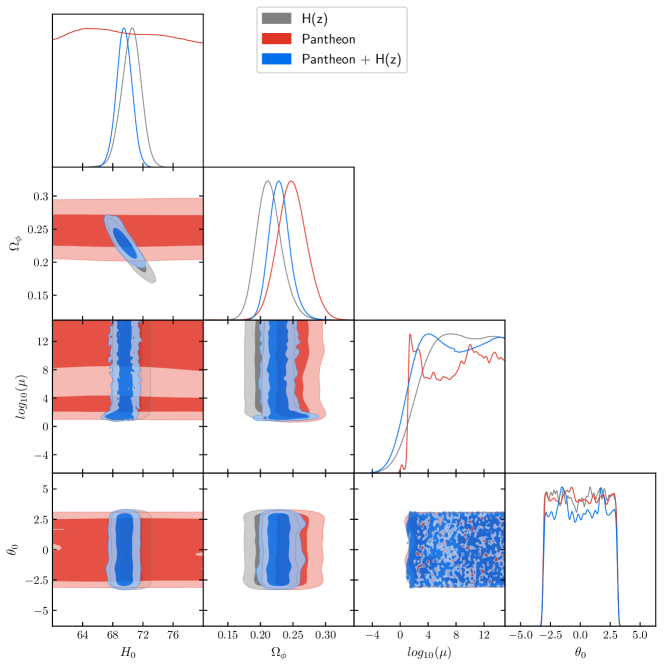
Figure 1: Constraints from Pantheon SNe Ia and $H(z)$.

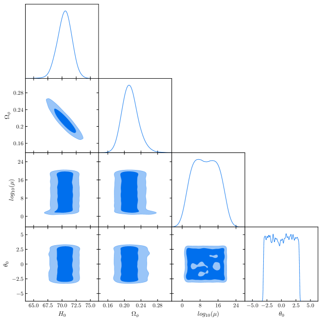
Figure 2: Constraints from Pantheon SNe Ia and $H(z)$.

Parameter	95% limits
$H_{0}$	$69.5^{+2.0}_{-2.1}$
$\Omega_{\phi}$	$0.230^{+0.033}_{-0.031}$
$log_{10}(\mu)$	$>\,\,-1.28$
$\theta_{0}$	$0.0^{+3.0}_{-3.0}$

Table 1: Mean Parameter Values

VI Concluding remarks

We have studied the SFDM model, which hypothesizes the description of dark matter by a real scalar field $\phi$. Taking a potential of the free field type, we have performed an statistical analysis of the model using tools such as the JWKB approximation, which allowed the numerical integrations of the (7)–(8) system to be executed for high values of $\mu$ faster than the exact solution. In the statistical analysis, the use of the MCMC method guaranteed greater precision in the results of the analysis of the $51$ data of $H(z)$ and the Pantheon sample of the SNe Ia data.

We have established limits for the free parameters of the model, obtaining a lower limit for the mass of the dark matter particle of about $10^{-34}\text{ eV}$ with $2\sigma$ confidence, a value close to what was found in js ; Marsh ($\approx 10^{-33}$ eV). In our analysis, we have also obtained $H_{0}=69.5^{+2.0}_{-2.1}$ km s^-1Mpc^-1. The value of $\Omega_{\phi}=0.230^{+0.033}_{-0.031}$ found and, together with the well-known $\Omega_{b}=0.032^{+0.092}_{-0.097}$, corresponding to baryonic matter in the universe, provides a total of $\Omega_{M}=0.262^{+0.098}_{-0.102}$. Both results for $H_{0}$ and $\Omega_{M}$ are compatible with the result found by Planck, of $H_{0}=67.4\pm 0.5$ km s^-1Mpc^-1 and $\Omega_{M}=0.315\pm 0.007$.

The SFDM model was satisfactory in describing astronomical observations reproducing results compatible with $\Lambda$CDM model and yet, when the mass of dark matter is very high, the SFDM model tends to $\Lambda$CDM. The advantage of the alternative model is in the explanation of some small scale CDM problems pp , like the cuspy/core problem. Since the dark matter particles form Bose-Einstein condensates very early in the evolution of the universe due to their low mass, it leads to the creation of a flat density profile in the center of galaxies 2 .

We have seen that the real scalar field $\phi$ proved to be a promising candidate for dark matter, although further analysis and testing should be done with the model to refine its results, for instance, by using CMB data that carries information from the primordial Universe.

- (1) L. Perivolaropoulos, arXiv:0811.4684 [astro-ph].
- (2) A. Del Popolo and M. Le Delliou, Galaxies 5 (2017) no.1, 17 [arXiv:1606.07790 [astro-ph.CO]].
- (3) S. Weinberg, The Cosmological Constant Problem, Rev. Mod. Phys. 61 (1989) 1.
- (4) S. Weinberg, astro-ph/0005265.
- (5) A. H. Guth, The Inflationary Universe The Quest for a New Theory of Cosmic Origins, Perseus Books. (1997)
- (6) Andrew R. Liddle, David H. Lyth, Cosmological inflation and large scale structure, Cambridge University Press. (2000)
- (7) Alan H. Guth, Phys. Rev. D 23, 347 (1981)
- (8) A.D. Linde. Physics Letters B. A new inflationary universe scenario: A possible solution of the horizon, flatness, homogeneity, isotropy and primordial monopole problems. Physics Letters B108 (1983) 389:393.
- (9) R. R. Caldwell, R. Dave and P. J. Steinhardt, Phys. Rev. Lett. 80 (1998) 1582 [astro-ph/9708069].
- (10) S. M. Carroll, Phys. Rev. Lett. 81 (1998) 3067 [astro-ph/9806099].
- (11) L. M. Wang, R. R. Caldwell, J. P. Ostriker and P. J. Steinhardt, Astrophys. J. 530 (2000) 17 [astro-ph/9901388].
- (12) B. Ratra and P. J. E. Peebles, Phys. Rev. D 37 (1988) 3406.
- (13) P. J. E. Peebles and B. Ratra, Astrophys. J. 325 (1988) L17.
- (14) T. Matos, A. Vázquez-González and J. Magaña, MNRAS 393, 1359 (2009).
- (15) J. Magana and T. Matos, A brief Review of the Scalar Field Dark Matter model, J. Phys. Conf. Ser. 378, 012012 (2012) [arXiv:1201.6107 [astro-ph.CO]].
- (16) J. F. Jesus, S. H. Pereira, J. L. G. Malatrasi and F. Andrade-Oliveira, JCAP 1608 (2016) no.08, 046 [arXiv:1504.04037 [gr-qc]].
- (17) T. Matos and F. S. Guzman, Class. Quant. Grav. 17, L9 (2000) [gr-qc/9810028]. 4
- (18) T. Matos and L. A. Urena-Lopez, Phys. Rev. D 63, 063506 (2001) [astro-ph/0006024].
- (19) H. I. Ringermacher and L. R. Mead, Astron. J. 149, 137 (2015).
- (20) N. Suzuki et al., Astrophys. J. 746, 85 (2012) [arXiv:1105.3470 [astro-ph.CO]].
- (21) G. S. Sharov and E. G. Vorontsova, JCAP10, 057 (2014), [arXiv:1407.5405 [gr-qc]].
- (22) G. D’Agostini, Bayesian reasoning in data analysis: a critical introduction. World Scientific Publishing (2003)
- (23) P. C. Gregory, Bayesian Logical Data Analysis for the Physical Sciences: A Comparative Approach with ‘Mathematica’ Support. Cambridge University Press (2005)
- (24) A. Gelman et al., “Bayesian Data Analysis”, CRC Press, Taylor & Francis Group (2014).
- (25) W. R. Gilks, S. Richardson e D. J. Spiegelhalter (eds.), “Markov Chain Monte Carlo in Practice”, London, UK: Chapman & Hall/CRC (1996)
- (26) J. Goodman e J. Weare, Comm. App. Math. Comp. Sci., v. 5, 1, 65 (2010)
- (27) Foreman, D. et al., 2013, Publ. Astron. Soc. Pac. 125 306 [arXiv:1202.3665 [astro-ph.IM]].
- (28) B. Ratra, Phys. Rev. D 44 (1991) 352.
- (29) Jeffreys, H. (1925), On Certain Approximate Solutions of Lineae Differential Equations of the Second Order. Proceedings of the London Mathematical Society, s2-23: 428-436.
- (30) J. Magana, M. H. Amante, M. A. Garcia-Aspeitia and V. Motta, Mon. Not. Roy. Astron. Soc. 476 (2018) no.1, 1036 [arXiv:1706.09848 [astro-ph.CO]].
- Simon et al. (2005) Simon, J. et al., Phys. Rev. D 71 (2005) 123001 [astro-ph/0412269].
- Stern et al. (2010) Stern, D. et al., J. of Cosmology and Astropart. Phys. 02 (2010) 008 [arXiv:0907.3149].
- Moresco et al. (2012) Moresco, M. et al., J. of Cosmology and Astropart. Phys. 8 (2012) 006 [arXiv:1201.3609].
- Zhang et al. (2012) Zhang, C. et al., Res. Astron. Astrophys. 14, no. 10, 1221 (2014) [arXiv:1207.4541 [astro-ph.CO]].
- Moresco (2015) Moresco, M., Mon. Not. Roy. Astron. Soc. 450 (2015) L16 [arXiv:1503.01116].
- Moresco et al. (2016) Moresco, M. et al., JCAP 1605 (2016) no.05, 014 [arXiv:1601.01701 [astro-ph.CO]].
- Gaztañaga et al. (2009) Gaztañaga, E. et al., Mon. Not. Roy. Astron. Soc. 399(3) (2009) 1663 [arXiv:0807.3551].
- Blake et al. (2012) Blake, C. et al., Mon. Not. Roy. Astron. Soc. 425(1) (2012) 405 [arXiv:1204.3674].
- Busca et al. (2012) Busca, N. G., et al., Astron. Astrophys. 552 (2013) A96 [arXiv:1211.2616].
- Anderson et al. (2013) Anderson, L. et al., Mon. Not. Roy. Astron. Soc. 439, no. 1, 83 (2014) [arXiv:1303.4666 [astro-ph.CO]].
- Font-Ribeira et al. (2013) Font-Ribera, A. et al., J. of Cosmology and Astroparticle Phys. 05 (2014) 027 [arXiv:1311.1767].
- Delubac et al. (2014) Delubac, T. et al. [BOSS Collaboration], Astron. Astrophys. 574 (2015) A59 [arXiv:1404.1801 [astro-ph.CO]].
- Chuang & Wang (2013) Chuang, C.H. and Wang, Y., Mon. Not. Roy. Astron. Soc. 435(1) (2013) 255 [arXiv:1209.0210].
- Oka et al. (2014) Oka, A. et al., Mon. Not. Roy. Astron. Soc. 439(3) (2014) 2515 [arXiv:1310.2820].
- (45) Riess, A.G. et al., Astrophys. J. 826 (2016) no.1, 56 [arXiv:1604.01424 [astro-ph.CO]].
- (46) Ade, P.A.R. et al. [Planck Collaboration], Astron. Astrophys. 594 (2016) A13 [arXiv:1502.01589 [astro-ph.CO]].
- (47) Bernal, J.L., Verde, L. and Riess, A.G., JCAP 1610 (2016) no.10, 019 [arXiv:1607.05617 [astro-ph.CO]].
- (48) J. A. S. Lima, J. F. Jesus, R. C. Santos and M. S. S. Gill, arXiv:1205.4688 [astro-ph.CO].
- (49) D. M. Scolnic et al., Astrophys. J. 859 (2018) no.2, 101 [arXiv:1710.00845 [astro-ph.CO]].
- (50) J. Guy et al. [SNLS Collaboration], Astron. Astrophys. 523 (2010) A7 [arXiv:1010.4743 [astro-ph.CO]].
- (51) M. Betoule et al. [SDSS Collaboration], Astron. Astrophys. 568 (2014) A22 [arXiv:1401.4064 [astro-ph.CO]].
- (52) R. Tripp, Astron. Astrophys. 331 (1998) 815.
- (53) J. Goodman, and J. Weare, Comm. App. Math. Comp. Sci., (2010) v.5, 1, 65
- (54) D. Foreman-Mackey, D. W. Hogg, D. Lang and J. Goodman, Publ. Astron. Soc. Pac. 125 (2013) 306 [arXiv:1202.3665 [astro-ph.IM]].
- (55) Allison, R. and Dunkley, J., Mon. Not. Roy. Astron. Soc. 437, 2014, no.4, 3918 [arXiv:1308.2675 [astro-ph.IM]].
- (56) A. Lewis and S. Bridle, Phys. Rev. D 66 (2002) 103511 [astro-ph/0205436].
- (57) Marsh, David J. E. and Ferreira, Pedro G., Ultra-Light Scalar Fields and the Growth of Structure in the Universe, Phys. Rev., D82 , 2010, [10.1103/PhysRevD.82.103528]. [arXiv:1104.5614 [astro-ph.CO]].
- (58) Bernabei, R. and others, First results from DAMA/LIBRA and the combined results with DAMA/NaI, DAMA ,Eur. Phys. J., C56,333-355, 2008.
- (59) Von Harling, Benedict and Petraki, Kalliopi, Bound-state formation for thermal relic dark matter and unitarity, JCAP, 1412, 2014.