An updated discussion of the solar abundance problem

Abstract

We discuss the level of agreement of a new generation of standard solar models (SSMs), Barcelona 2016 or B16 for short, with helioseismic and solar neutrino data, confirming that models implementing the AGSS09met surface abundances, based on refined three-dimensional hydrodynamical simulations of the solar atmosphere, do not not reproduce helioseismic constraints. We clarify that this solar abundance problem can be equally solved by a change of the composition and/or of the opacity of the solar plasma, since effects produced by variations of metal abundances are equivalent to those produced by suitable modifications of the solar opacity profile. We discuss the importance of neutrinos produced in the CNO cycle for removing the composition-opacity degeneracy and the perspectives for their future detection.

1 Introduction

In the last three decades, there was an enormous progress in our understanding of the Sun. The predictions of the Standard Solar Model (SSM), which is the fundamental theoretical tool to investigate the solar interior, have been tested by solar neutrino experiments and by helioseismology. The deficit of the observed solar neutrino fluxes, reported initially by Homestake[1, 2] and then confirmed by GALLEX[3], SAGE[4], GNO[5], Kamiokande[6] and Super-Kamiokande[7], generated the so-called “solar neutrino problem” which stimulated a deep investigation of the solar structure. The problem was solved in 2002 when the SNO experiment[8] obtained a direct evidence for flavour oscillations of solar neutrinos and, moreover, confirmed the SSM prediction of the ${}^{8}{\rm B}$ neutrino flux.

Nowadays, we have a good knowledge of the solar neutrino oscillation probability and a direct experimental determination of most of the solar neutrino components. Super-Kamiokande[9] and SNO[10] have provided a high accuracy determination of ${}^{8}{\rm B}$ neutrinos. Borexino[11, 12, 13] has recently obtained a direct measure of the pp, pep, ${}^{7}{\rm Be}$ and ${}^{8}{\rm B}$ solar neutrino fluxes and it also has the potential to provide the first direct measurements of the CNO neutrinos[14] in the next future. In addition, helioseismic observations have allowed to determine precisely several important properties of the Sun, such as the depth of the convective envelope which is known at the $\sim 0.2\%$ level, the surface helium abundance which is obtained at the $\sim 1.5\%$ level and the sound speed profile which is determined with an accuracy equal to $\sim 0.1\%$ in a large part of the Sun (see e.g. Refs.15 and 16 and J. Christensen-Dalsgaard contribution to these proceedings. As a results of these observations, the solar structure is now very well constrained, so that the Sun can be used as a solid benchmark for stellar evolution and as a “laboratory” for fundamental physics.

A new solar problem has, however, emerged during the last years. Recent determinations of the photospheric heavy element abundances[17, 18, 19] indicate that the Sun metallicity is lower than previously assumed[20, 21]. Solar models that incorporate these lower abundances are no more able to reproduce the helioseismic results. As an example, the sound speed predicted by SSMs at the bottom of the convective envelope disagrees at the $\sim 1\%$ level with the value inferred by helioseismic data (see e.g. Ref.22). Detailed studies have been done to resolve this controversy (see e.g. Ref.23), but a definitive solution of this solar abundance problem still has to be obtained.

In this review, we provide a quantitative discussion of the solar abundance problem. The plan of the paper is as follows. In Secs.2 and 3, we present a a new generation of standard solar models (SSMs), Barcelona 2016 or B16 for short, and we quantify the level of agreement of models implementing different surface abundances with helioseismic and solar neutrino data. In Sec.4, we discuss the degeneracy between the effects produced by a modification of the radiative opacity and of those produced by a modification of the surface composition. In Sec.5, we dicsuss the importance of neutrinos produced in the CNO cycle for removing the composition-opacity degeneracy and for solving the solar abundance problem. Finally, we summarise our results in Sec.6.

2 The B16 standard solar models

SSMs are a snapshot in the evolution of a 1$M_{\odot}$ star, calibrated to match present-day surface properties of the Sun. The calibration is done by adjusting the mixing length parameter ($\alpha_{\rm MLT}$) and the initial helium and metal mass fractions ($Y_{\rm ini}$ and $Z_{\rm ini}$ respectively) in order to satisfy the constraints imposed by the present-day solar luminosity $L_{\odot}$, radius $R_{\odot}$, and surface metal to hydrogen abundance ratio $(Z/X)_{\odot}$. The new B16 models share with previous calculations[24] much of the input physics, but include important updates. A brief account of few relevant ingredients is given in the following.

Equation of State: B16 SSMs employ, for the first time, EoS tables calculated consistently for each of the compositions used in the solar calibrations by using FreeEOS[25].

Nuclear rates: The rates of ${\rm p(p,e^{+}\nu_{e})d}$, ${\rm{}^{\rm 7}Be(p,\gamma)^{\rm 8}B}$ and ${\rm{}^{\rm 14}N(p,\gamma)^{\rm 15}O}$ reactions have been updated, see Tab.2. For the important reaction ${}^{3}{\rm He}(^{4}{\rm He},\gamma)^{7}{\rm Be}$ (not included in Tab.2), two recent analyses[27, 28] have provided determinations of the astrophysical factor that differs by about $6\%$ (to be compared with a claimed accuracy equal to $4\%$ and $2\%$ for Refs. 27 and 28, respectively). Considering that the results from Refs.27 and 28 bracket the previously adopted value from Ref.29, the latter was considered as preferred choice in B16 SSMs.

Astrophysical S-factors (in units of MeV b) and uncertainties updated in this work. Fractional changes with respect to Ref.29 are also included. S(0) Uncert.(%) $\Delta S(0)/S(0)$ Ref. $\rm{S_{11}}$ $4.03\cdot 10^{-25}$ 1 0.5% 30, 31, 32 $\rm{S_{17}}$ $2.13\cdot 10^{-5}$ 4.7 +2.4% 33 $\rm{S_{114}}$ $1.59\cdot 10^{-3}$ 7.5 -4.2% 34

Radiative opacities: In Ref.24 the opacity error was modelled as a 2.5% constant factor at 1$\sigma$ level, comparable to the maximum difference between OP [35] and OPAL [36] opacities in the solar radiative region. It was shown, however, in Ref.37 that this prescription underestimates the contribution of opacity uncertainty to the sound speed and convective radius error budgets because the effects produced by opacity variations in different zones of the Sun compensate among each other and integrate to zero for a global rescaling of the opacity. Moreover this is not realistic because the accuracy of opacity calculations is expected to be better at the solar core than in the region around the base of the convective envelope. Taking this into account, the following parameterization for the opacity change $\delta\kappa(T)$ was considered:

$$\delta\kappa(T)=a+b\frac{\log\left(T_{\rm C}/T\right)}{\Delta}$$ (1)

where $T$ is the temperature of the solar plasma, $\Delta=\log\left(T_{\rm C}/T_{\rm CZ}\right)=0.9$, $T_{\rm C}=15.6\times 10^{6}\,{\rm K}$ and $T_{\rm CZ}=2.3\times 10^{6}\,{\rm K}$ are the temperatures at the solar center and at the bottom of the convective zone respectively. The parameters $a$ and $b$ are treated as independent random variables with mean equal to zero and dispersions $\sigma_{a}=2\%$ and $\sigma_{b}=6.7\%$, respectively. This corresponds to assuming that the opacity error at the solar center is $\sigma_{\rm in}=\sigma_{a}=2\%$ , while it is given by $\sigma_{\rm out}=(\sigma_{a}^{2}+\sigma_{b}^{2})^{1/2}=7\%$ at the base of the convective zone, as can be motivated by the recent experimental results of Ref.38 and the theoretical work by Ref.39.

Surface composition: The solar surface composition is a fundamental constraint in the construction of SSMs. In this paper, we consider two different canonical sets of solar abundances which are the same employed in Ref.24:

• GS98 - Photospheric (volatiles) + meteoritic (refractories) abundances from Ref.20 that correspond to metal-to-hydrogen ratio used for the calibration $(Z/X)_{\odot}=0.0229$;

• AGSS09met - Photospheric (volatiles) + meteoritic (refractories) abundances from Ref.17 that give $(Z/X)_{\odot}=0.0178$.

Note that the recent results from Refs.40, 41, 42 that have updated the abundances of Ref.17 for all but CNO elements (which are the most abundant among the volatiles elements) do not lead to a revision of the AGSS09met composition.

Neutrino fluxes for the two B16 SSMs and as determined by Ref.43. The fluxes are given in units of $10^{10}\,(\rm{pp})$, $10^{9}\,(\rm{{}^{7}Be})$, $10^{8}\,(\rm{pep,^{13}N,^{15}O})$, $10^{6}\,(\rm{{}^{8}B,^{17}F})$ and $10^{3}\,(\rm{hep})$ $\rm{cm^{-2}s^{-1}}$. The last two lines give the surface helium $Y_{\rm S}$ and the convective radius $R_{\rm CZ}$. The observational values are given by Refs. 44 and 45, respectively. GS98 AGSS09met Obs $\Phi({\rm pp})$ $5.98(1\pm 0.006)$ $6.03(1\pm 0.005)$ $5.971^{+0.037}_{-0.033}$ $\Phi({\rm pep})$ $1.44(1\pm 0.01)$ $1.46(1\pm 0.009)$ $1.448\pm 0.013$ $\Phi({\rm hep})$ $7.98(1\pm 0.30)$ $8.25(1\pm 0.30)$ $19^{+12}_{-9}$ $\Phi(^{7}{\rm Be})$ $4.93(1\pm 0.06)$ $4.50(1\pm 0.06)$ $4.80^{+0.24}_{-0.22}$ $\Phi(^{8}{\rm B})$ $5.46(1\pm 0.12)$ $4.50(1\pm 0.12)$ $5.16^{+0.13}_{-0.09}$ $\Phi(^{13}{\rm N})$ $2.78(1\pm 0.15)$ $2.04(1\pm 0.14)$ $\leq 13.7$ $\Phi(^{15}{\rm O})$ $2.05(1\pm 0.17)$ $1.44(1\pm 0.16)$ $\leq 2.8$ $\Phi(^{17}{\rm F})$ $5.29(1\pm 0.20)$ $3.26(1\pm 0.18)$ $\leq 85$ $Y_{\rm S}$ $0.2426\pm 0.0059$ $0.2317\pm 0.0059$ $0.2485\pm 0.0035$ $R_{\rm CZ}$ $0.7116\pm 0.0048$ $0.7223\pm 0.0053$ $0.713\pm 0.001$

3 B16-SSMs results

The main results obtained with the new generation of B16 SSMs for the two choices of solar composition, GS98 and AGSS09met, are shown in Tab.2, Fig.1 and 2 and are discussed below. In Tab. 3 we quantify the level of agreement between the B16-SSMs predictions and different ensembles of solar observables. The $\chi^{2}$ values reported in Tab.3 are calculated by including experimental and theoretical (correlated) uncertainties as described in Refs.46 and 26.

Neutrino fluxes: The updates of nuclear reaction rates have a direct effect on neutrino production. In particular, the boron and beryllium neutrino fluxes are reduced for both GS98 and AGSS09met compositions by about 2% with respect to previous SSM calculations [24]. The overall reduction in the $\Phi(^{8}{\rm B})$ and $\Phi(^{8}{\rm Be})$ fluxes comes from the increase in $S_{11}$. In the case of $\Phi(^{8}{\rm B})$, this is partially compensated by the 2.4% increase in $S_{17}$. The most important changes in the neutrino fluxes occur for $\Phi(^{13}{\rm N})$ and $\Phi(^{15}{\rm O})$, in the CN-cycle. The expectation values in the B16 SSMs are about 6% and 8% lower than for the previous SSMs [24]. This results from the combined changes in the p+p and ¹⁴N+p reaction rates.

The predicted fluxes should be compared with the observational values in the last column of Tab.2 which have been obtained in Ref.43 from a fit to the results of solar neutrino experiments by allowing for three-flavour neutrino oscillations. Note that observational errors for $\Phi(^{8}{\rm B})$ and $\Phi(^{8}{\rm Be})$ fluxes are smaller than uncertainties in theoretical predictions, as can be also appreciated in Fig.1 where we summarize the present situation for these two components of the solar neutrino spectrum. On the contrary, CN fluxes have not yet been determined experimentally and the global analysis of solar neutrino data provides only the upper limits included in Tab.2.

From the quantitative comparison of B16-GS98 and B16-AGSS09met predictions with the experimentally inferred neutrino fluxes, we conclude that both calculations are consistent with neutrino data within $1\sigma$. We obtain indeed $\chi^{2}/{\rm dof}\lesssim 1$ for both assumed compositions when considering $\Phi(^{7}{\rm Be})+\Phi(^{8}{\rm B})$ and/or “all $\nu$-fluxes” experimental deteminations, as it is reported in Tab.3.

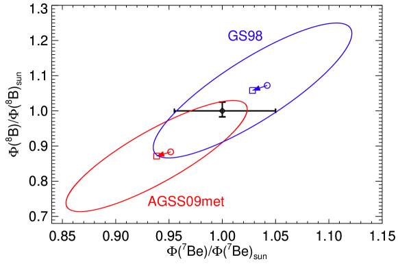
Figure 1: $\Phi({\rm{}^{8}B})$ and $\Phi({\rm{}^{7}Be})$ fluxes normalized to the solar values obtained in Ref.43. Black circle and error bars: solar values. Squares and circles: results for B16 (current) and (older) generation of SSMs respectively. Ellipses denote theoretical 1$\sigma$ C.L. for 2 dof.

Helioseismology: In the last two lines of Tab.2, we report two helioseismic quantities widely used in assessing the quality of SSMs, i.e. the surface helium abundance $Y_{\rm S}$ and the depth of the convective envelope $R_{\rm CZ}$, together with the corresponding seismically determined values. The model errors associated to these quantities are larger than previously computed because of the different treatment of uncertainties in radiative opacities. Compared to previous SSMs[24], we find a small decrease in the predicted $Y_{\rm S}$ by 0.0003 and in the predicted $R_{\rm CZ}$ by $0.0007R_{\odot}$ for both compositions. These small changes together with the larger theoretical uncertainties lead B16-GS98 to a 0.9$\sigma$ ($Y_{\rm S}$) and 0.3$\sigma$ ($R_{\rm CZ}$) difference with respect to data while for B16-AGSS09met differences are at the 2.5$\sigma$ ($Y_{\rm S}$) and 1.7$\sigma$ ($R_{\rm CZ}$) level. When combined together, see Tab.3, these helioseismic observables give a $\chi^{2}$ (for 2 dof) equal to 0.9 (6.5) for B16-GS98 (B16-AGSS09met) predictions, showing a preference for the high metallicity assumption.

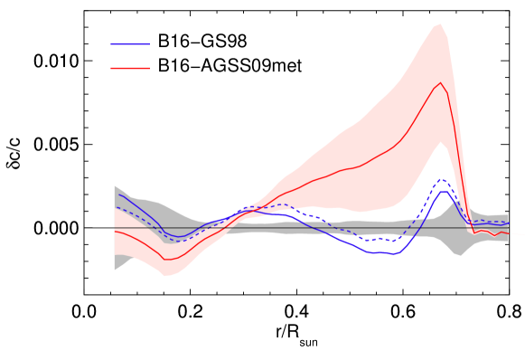
Figure 2: Fractional sound speed difference $\delta{\rm c/c=(c_{\odot}-c_{\rm SSM})/c_{\rm SSM}}$. The grey shaded region corresponds to errors in the helioseismic inversion procedure. The red shaded region around the AGSS09met central value (solid red line) describes uncertainties in SSM calculations. An equivalent relative error band holds around the central value of the GS98 central value (solid blue line) which we do not plot for the sake of clarity. Dashed line shows, for comparison, results for old SSM calculations [24].

Finally, Fig.2 shows the fractional difference between the sound speed inferred from helioseismic frequencies and that predicted by B16 SSMs as a function of solar radius for the two choices of solar composition. The solar sound speed has been obtained by new inversions based on the so-called BiSON-13 dataset [47] and using consistently both B16 SSMs as reference models. Results are only slightly different with respect to previous calculations, mainly as a result of the updated $S_{11}(0)$ value. The red shaded region around the AGSS09met central value (solid red line) describes theoretical uncertainties in SSM calculations. An equivalent relative error band holds around the central value of the GS98 central value (solid blue line) which we do not plot for the sake of clarity. The sound speed profile is also affected by observational errors which are due to uncertainties in the measured helioseismic frequencies, numerical parameters inherent to the inversion procedure and the solar model used as a reference model for performing the inversion. These errors have been evaluated as described in Refs.15 and 26 and correspond to the grey shaded region in Fig.2

We see that B16-GS98 model yields a much better agreement, everywhere in the solar structure, with the helioseismically derived sound speed profile than B16-AGSS09met. In particular, the B16-AGSS09 model disagrees by $\sim 1\%$ with sound speed inferred from helioseismology at the bottom of the convective envelope. This has to be compared with a theoretical uncertainty of $\sim 0.3\%$ and an error in the inversion procedure smaller than $0.1\%$. Using theoretical and experimental uncertainties as described in Ref.46, we can compare how well the predicted sound speed profiles of B16-GS98 and B16-AGSS09met agree with helioseismic inferences. For this, we use the same 30 radial points employed in Refs.46. Results are shown in the second row of Tab.3. For 30 degrees-of-freedom (dof), B16-GS98 gives $\chi^{2}=58$, or a $3.2\sigma$ agreement with data. For B16-AGSS09met results are $\chi^{2}=76.1$, or $4.5\sigma$. It is important to notice that in the case of B16-GS98, the largest contribution to the sound speed $\chi^{2}$ comes from the narrow region $0.65<r/R_{\odot}<0.70$ that comprises 2 out of all the 30 points. If these two points are removed from the analysis $\chi^{2}$ is reduced from 58 to 34.7, equivalent to a $1.4\sigma$ agreement with the solar sound speed (entry identified as $\delta c/c$ no-peak in Tab.3). For B16-AGSS09met this test leads to a $2.7\sigma$ result. This exercise highlights the qualitative difference between SSMs with different compositions; it shows that for GS98 the problem is highly localized whereas for AGSS09met the disagreement between SSMs and solar data occurs at a global scale, i.e. the solar abundance problem.

Comparison of B16 SSMs against different ensembles of solar observables. GS98 AGSS09met Case dof $\chi^{2}$ p-value $(\sigma)$ $\chi^{2}$ p-value $(\sigma)$ $Y_{\rm S}+R_{\rm CZ}$ only 2 0.9 0.5 6.5 2.1 $\delta c/c$ only 30 58.0 3.2 76.1 4.5 $\delta c/c$ no-peak 28 34.7 1.4 50.0 2.7 $\Phi({\rm{}^{7}Be})+\Phi({\rm{}^{8}B})$ 2 0.2 0.3 1.5 0.6 all $\nu$-fluxes 8 6.0 0.5 7.0 0.6 global 40 65.0 2.7 94.2 4.7 global no-peak 38 40.5 0.9 67.2 3.0

4 The opacity-composition degeneracy

The interpretation of the solar abundance problem is complicated by the degeneracy between effects produced by a modification of the radiative opacity $\kappa(\rho,T,Y,Z_{\rm i})$ and effects induced by a change of the heavy element admixture $\{z_{\rm i}\}$, expressed here in terms of the quantities $z_{\rm i}\equiv Z_{\rm i,b}/X_{\rm b}$ where $Z_{\rm i,b}$ is the surface abundance of the $i$-element and $X_{\rm b}$ is that of hydrogen.

This degeneracy was discussed in quantitative terms in Ref.37 by using the linear solar model (LSM) approach introduced in Ref.48. By neglecting the role of metals in the equation of state and in the energy generation coefficient, it was shown that the source term $\delta\kappa(r)$ that drives the modification of the solar properties and that can be constrained by observational data can be written as the sum of two contributions:

$$\delta\kappa(r)=\delta\kappa_{\rm I}(r)+\delta\kappa_{\rm Z}(r)$$ (2)

The first term $\delta\kappa_{\rm I}(r)$, which we refer to as intrinsic opacity change, represents the fractional variation of the opacity along the solar profile and it is given by:

$$\delta\kappa_{\rm I}(r)=\frac{\kappa(\overline{\rho}(r),\overline{T}(r),\overline{Y}(r),\overline{Z}_{i}(r))}{\overline{\kappa}(\overline{\rho}(r),\overline{T}(r),\overline{Y}(r),\overline{Z}_{i}(r))}-1$$ (3)

where the notation $\overline{Q}$ indicates, here and in the following, the value for the generic quantity $Q$ that is obtained in a reference SSM calculation. This contribution is obtained when we revise the opacity function $\kappa(\rho,T,Y,Z_{\rm i})$ and/or we introduce new effects, like e.g. the accumulation of few GeVs WIMPs in the solar core that mimics a decrease of the opacity at the solar center, see e.g. Ref.49 and references therein. The second term $\delta\kappa_{\rm Z}(r)$, which we refer to as composition opacity change, describes the effects of a variation of $\left\{z_{\rm i}\right\}$. It takes into account that a modification of the photospheric admixture implies a different distribution of metals inside the Sun and, thus, a different opacity profile, even if the function $\kappa(\rho,T,Y,Z_{\rm i})$ is unchanged. The contribution $\delta\kappa_{\rm Z}(r)$ is given by:

$$\delta\kappa_{\rm Z}(r)=\frac{\overline{\kappa}(\overline{\rho}(r),\overline{T}(r),\overline{Y}(r),Z_{i}(r))}{\overline{\kappa}(\overline{\rho}(r),\overline{T}(r),\overline{Y}(r),\overline{Z}_{i}(r))}-1$$ (4)

where $Z_{\rm i}(r)\simeq\overline{Z}_{\rm i}(r)\,(z_{\rm i}/\overline{z}_{\rm i})$ and can be calculated as:

$$\delta\kappa_{\rm Z}(r)\simeq\sum_{i}\left.\frac{\partial\ln\overline{\kappa}}{\partial\ln Z_{i}}\right|_{\rm SSM}\;\delta z_{\rm i,b}$$ (5)

where $\delta z_{\rm i}$ represents the fractional variation of $z_{\rm i}$ and the symbol $|_{\rm SSM}$ indicates that we calculate the derivatives along the density, temperature and chemical composition profiles predicted by the reference SSM. Equation (2), although being approximate, is quite useful because it makes explicit the connection (and the degeneracy) between the effects produced by a modification of the radiative opacity and of those produced by a modification of the heavy element admixture.

The response of the Sun to an arbitrary modification of the opacity $\delta\kappa(r)$ was studied in Ref.37 (see also Refs.50 and 26) by computing numerically the kernels that, in a linear approximation, relate the opacity change $\delta\kappa(r)$ to the corresponding modifications of the solar observable properties. The following quantities where considered: the sound speed profile, the surface helium abundance, the inner boundary of the convective envelope, the solar neutrino fluxes, the central solar temperature. It was shown that different observable quantities probe different regions of the Sun. Moreover, effects produced by variations of opacity in distinct zones of the Sun may compensate among each other. In this respect, it was noted that the sound speed profile and the depth of the convective envelope are practically insensitive to a global rescaling of the opacity. As a consequence, the discrepancy between the helioseismic determinations of these quantities and the predictions of SSMs implementing AGSS09met composition can be equally solved by a $\sim 15\%$ decrease of the opacity a the center of the Sun or by a $\sim 15\%$ increase of the opacity in the external radiative region. The degeneracy between these two possible solutions is, however, broken by the “orthogonal” information provided by the measurements of the surface helium abundance and of the boron and beryllium neutrino fluxes, that fix the scale of opacity and indicate that only the second possibility can effectively solve the solar composition problem.

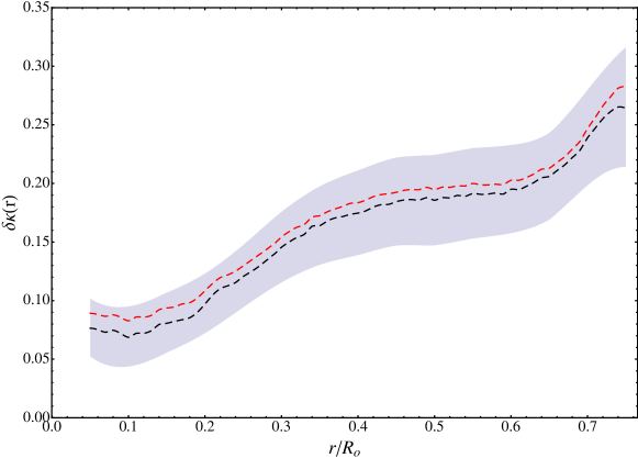
Figure 3: The effective opacity change $\delta\kappa(r)$ of solar models that provide a good fit to helioseismic and solar neutrino data when $\left(\delta z_{\rm CNO},\delta z_{\rm Ne},\delta z_{\rm met}\right)$ are allowed to vary. The black dashed line correspond to the best fit model. The red dashed line correspond to the best fit model obtained with the additional assumption that $\delta Z_{\rm Ne}=\delta z_{\rm CNO}$, i.e. that the neon-to-oxygen ratio is equal to the value prescribed by AGSS09met compilation. See Ref.46 for details.

Incidentally, the above conclusion is confirmed by the analysis presented in Ref.46 where helioseismic and solar neutrino data are used to infer the optimal composition of the Sun. The effective opacity change $\delta\kappa(r)$ (with respect to reference SSM implementing AGSS09met surface composition and OP opacity[35]) that produces a good fit to observational data is shown in Fig.3. We see that $\delta\kappa(r)$ is well constrained by the available observational information. Opacity should be increased by $\sim{\rm few}$ percent at the center of the Sun and by $\sim 25\%$ at the bottom of the convective envelope, as it was calculated by Ref37. The red dashed line in Fig.3 is obtained in a two parameter analysis in which elements are grouped as volatiles (i.e., C, N, O, and Ne) and refractories (i.e., Mg, Si, S, and Fe). The optimal surface composition is found by increasing the abundance of volatiles by $(45\pm 4)\%$ and that of refractories by $(19\pm 3)\%$ with respect to the values provided by AGSS09met. The black lines is obtained in a three parameter analysis in which the neon-to-oxygen ratio is allowed to vary within the currently allowed range (i.e., $\pm 30\%$ at $1\sigma$). The best-fit composition is obtained by increasing by $(37\pm 7)\%$ the CNO elements; by $(80\pm 26)\%$ the neon; and by $(13\pm 5)\%$ the refractory elements. We see that the two lines coincide at the 2% level or better. From this, we infer that the reconstructed opacity profile does not depend on the assumed heavy element grouping. Moreover, we understand that the best-fit compositions obtained in the two and three parameter analyses cannot be discriminated by the adopted observational constraints.

5 CNO neutrinos

As it is well known, the degeneracy between radiative opacity and solar composition can be removed by measuring the neutrino fluxes produced in the CNO cycle. The peculiarity of the CNO cycle is that it uses carbon, nitrogen and oxygen nuclei which are present in the core of the Sun as catalysts for H burning. As a consequence, its contribution to neutrino and energy production, beside depending on the solar temperature stratification (and thus on the opacity profile of the Sun), is approximately proportional to the stellar-core number abundance of CNO elements. This additional dependence can be used in combination with other helioseismic and solar neutrino probes to obtain a direct determination of the CNO core abundances.

This possibility was discussed on a quantitative basis in Ref.51. By taking advantage of the fact that $\Phi(^{13}{\rm N})$ and $\Phi(^{15}{\rm O})$ fluxes, which are produced by the dominant CN-branch of the CNO cycle, have a similar dependence on the core temperature of ⁸B neutrinos, it was shown that the measured $\Phi(^{8}{\rm B})$ flux can be used to largely eliminate environmental uncertainties (solar age, opacity, luminosity,…) affecting the CN fluxes predictions. This permits to translate a future measurement of CN neutrinos into a determination of the carbon and nitrogen abundances in the solar core with an accuracy that is sufficient to discriminate between opacity and/or composition changes as the solution of the solar abundance problem. Moreover, by directly comparing surface and core abundances one could, in principle, test the standard chemical evolution paradigm, according to which the Sun was born chemical homogenous and then it has evolved its internal composition due to nuclear reactions and elemental diffusion.

At present, we still miss a direct observational evidence for CNO energy generation in the Sun. We only have a loose upper limit on CNO neutrino fluxes obtained by combining the results of the various solar neutrino experiments. Direct detection of CNO neutrinos is a very difficult task. Not only the flux is relatively low, but also their energy is not large. The neutrinos produced by $\beta$-decay processes in the CNO cycle, i.e.

$${}^{13}{\rm N} \rightarrow {}^{13}{\rm C}+e^{+}+\nu_{e}$$

$${}^{15}{\rm O} \rightarrow {}^{15}{\rm N}+e^{+}+\nu_{e}$$ (6)

$${}^{17}{\rm F} \rightarrow {}^{17}{\rm O}+e^{+}+\nu_{e}$$

have continuous energy spectra with endpoints at about $\sim 1.5\,{\rm MeV}$. Differently from the monochromatic ⁷Be and pep solar neutrinos, they do not produce specific spectral features that permit to extract them unambiguously from the background event spectrum in high purity liquid scintillators. In particular, as it is shown in Fig.4, the electrons produced by the $\beta$-decay of Bismuth-210 to Polonium-210 have a spectrum that is similar to that produced by CNO neutrinos. As a consequence, spectral fits are able to determine only combined “Bismuth+CNO” contribution, as it is done e.g. by Borexino[52].

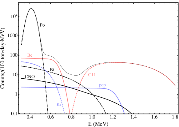
Figure 4: The expected event spectrum in solar neutrino liquid scintillator detectors calculated by assuming background levels and detector energy resolution comparable to those obtained by Borexino detector [53]. See Ref.14 for details.

In order to remove this degeneracy, a method to determine the Bi-210 decay rate which is based on the relationship between the Bi-210 and Po-210 abundances was proposed in Ref.14. Polonium-210, which is the Bismuth-210 daughter, is unstable and decays with a lifetime $\tau_{\rm Po}\sim 200$ days emitting a monochromatic $\alpha$ particle that can be easily detected. In the absence of Bismuth-210, the $\alpha$-decay rate of Po-210 nuclei follows the exponential decay law, $n_{\rm Po}(t)\propto\exp(-t/\tau_{\rm Po})$. The deviations from this behaviour can be used to determine the $\beta$-decay rate of Bi-210 nuclei. It was shown in Ref.14 that a Borexino-like detector could start discerning CNO neutrino signal in $\Delta t\sim 1{\rm yr}$, if the initial Po-210 event rate is $\sim 2000$cpd/100ton or lower. Future Kton-scale detectors, like e.g. SNO+, in the same time interval, could begin to discriminate between high and low metallicity solar models. The required assumptions are that the $\alpha$-particle detection efficiency is stable and external sources of Po-210 are negligible during the data acquisition period. This requires stabilizing the detector, avoiding in particular convective motions in the liquid scintillator that may bring additional Po-210 in the fiducial volume, over time scales comparable with the Polonium lifetime. The efforts of Borexino in this direction are described in D. Guffanti contribution to this Workshop.

Finally, we discuss a component of the solar neutrino spectrum which usually not included in solar neutrino analysis. As it was pointed out in Refs.54, 55 and then considered in Ref.56, along with neutrinos originating from the $\beta^{+}$ decay of ${}^{13}{\rm N}$, ${}^{15}{\rm O}$ and ${}^{17}{\rm F}$, neutrinos are also produced in the CNO cycle by the electron capture reactions:

$${}^{13}{\rm N}+e^{-} \rightarrow {}^{13}{\rm C}+\nu_{e}$$

$${}^{15}{\rm O}+e^{-} \rightarrow {}^{15}{\rm N}+\nu_{e}$$ (7)

$${}^{17}{\rm F}+e^{-} \rightarrow {}^{17}{\rm O}+\nu_{e}$$

The resulting fluxes, to which we refer as ecCNO neutrino fluxes, are extremely small, at the level of 0.1% with respect to the “conventional” CNO neutrino fluxes. However, ecCNO neutrinos are monochromatic and have larger energies equal to $E_{\nu}\sim 2.5\,{\rm MeV}$. In Ref.56, it was suggested suggest that these characteristics could make their detection possible in gigantic ultra-pure liquid scintillator detectors. The expected event rate is extremely low, at the level of few counts/1kton/year in the observation window between $E_{\rm vis}\simeq[1.5\,{\rm MeV},2.5\,{\rm MeV}]$ above the conventional CNO neutrinos endpoint, see Ref.56 for details. We thus understand that detectors with fiducial masses equal to $\sim 10\,{\rm kton}$ or more are necessary, for statistical reasons, to extract the ecCNO neutrino signal. Moreover, detectors should be placed underground at a depth comparable to Pyhasalmi and SNOLAB, in order to prevent a too large cosmogenic background. In conclusion, the determination of this sub-dominant component of the solar neutrino flux is extremely difficult but could be rewarding in terms of physical implications. Indeed, besides testing the efficiency of the CNO cycle and probing the metallic content of the solar core, it could also provide a determination of the electron neutrino survival probability at the energy $E_{\nu}\simeq 2.5\,{\rm MeV}$ which is otherwise inaccessible, with important implications for the final confirmation of the LMA-MSW flavour oscillation paradigm.

6 Summary

In this review, we have described the B16-SSMs that includes recent updates on some important nuclear reaction rates, a more consistent treatment of the equation of state and a novel and flexible treatment of opacity uncertainties. We have quantified the level of agreement of the B16-SSMs calculated with two different canonical sets of solar abundances, namely the (old, high metallicity) GS98 and the (new, low metallicity) AGSS09met composition, with the helioseismic determination of the sound speed profile, the depth of the convective envelope, the surface helium abundance and with solar neutrino data.

We have confirmed that solar models implementing the AGSS09met abundances, based on three-dimensional hydrodynamical simulations of the solar atmosphere (rather than the simplified one-dimensional static models used in the past), do not reproduce helioseismic constraints. We have argued that this solar abundance problem can be equally solved by a change of the composition and/or of the opacity of the solar plasma, since effects produced by variations of metal abundances are equivalent to those produced by suitable modifications of the solar opacity profile, as it is quantitatively expressed by Eq.2.

Finally, we have emphasised the importance of neutrinos produced in the CNO cycle, either the conventional CNO neutrinos produced by $\beta$-decay of ${}^{13}{\rm N}$, ${}^{15}{\rm O}$ , ${}^{17}{\rm F}$ or the less abundant ecCNO neutrinos produced by electron capture reactions on the same nuclei, for removing the composition-opacity degeneracy and we have discussed the perspective for their future detection.

References

- [1] R. Davis, Jr., D. S. Harmer and K. C. Hoffman, Search for neutrinos from the sun, Phys. Rev. Lett. 20, 1205 (1968).
- [2] B. T. Cleveland, T. Daily, R. Davis, Jr., J. R. Distel, K. Lande, C. K. Lee, P. S. Wildenhain and J. Ullman, Measurement of the solar electron neutrino flux with the Homestake chlorine detector, Astrophys. J. 496, 505 (1998).
- [3] W. Hampel et al., GALLEX solar neutrino observations: Results for GALLEX IV, Phys. Lett. B447, 127 (1999).
- [4] J. N. Abdurashitov et al., Measurement of the solar neutrino capture rate by SAGE and implications for neutrino oscillations in vacuum, Phys. Rev. Lett. 83, 4686 (1999).
- [5] M. Altmann et al., Complete results for five years of GNO solar neutrino observations, Phys. Lett. B616, 174 (2005).
- [6] K. S. Hirata et al., Observation of B-8 Solar Neutrinos in the Kamiokande-II Detector, Phys. Rev. Lett. 63, p. 16 (1989).
- [7] J. P. Cravens et al., Solar neutrino measurements in Super-Kamiokande-II, Phys. Rev. D78, p. 032002 (2008).
- [8] Q. R. Ahmad et al., Measurement of day and night neutrino energy spectra at SNO and constraints on neutrino mixing parameters, Phys. Rev. Lett. 89, p. 011302 (2002).
- [9] K. Abe et al., Solar Neutrino Measurements in Super-Kamiokande-IV, Phys. Rev. D94, p. 052010 (2016).
- [10] A. Bellerive, J. R. Klein, A. B. McDonald, A. J. Noble and A. W. P. Poon, The Sudbury Neutrino Observatory, Nucl. Phys. B908, 30 (2016).
- [11] G. Bellini et al., Neutrinos from the primary proton–proton fusion process in the Sun, Nature 512, 383 (2014).
- [12] M. Agostini et al., First Simultaneous Precision Spectroscopy of , 7Be, and Solar Neutrinos with Borexino Phase-II (2017).
- [13] M. Agostini et al., Improved measurement of 8B solar neutrinos with 1.5 kt y of Borexino exposure (2017).
- [14] F. L. Villante, A. Ianni, F. Lombardi, G. Pagliaroli and F. Vissani, A Step toward CNO solar neutrinos detection in liquid scintillators, Phys. Lett. B701, 336 (2011).
- [15] S. Degl’Innocenti, W. A. Dziembowski, G. Fiorentini and B. Ricci, Helioseismology and standard solar models, Astropart. Phys. 7, 77 (1997).
- [16] D. O. Gough et al., The seismic structure of the Sun, Science 272, 1296 (1996).
- [17] M. Asplund, N. Grevesse, A. J. Sauval and P. Scott, The chemical composition of the Sun, Ann. Rev. Astron. Astrophys. 47, 481 (2009).
- [18] E. Caffau, H.-G. Ludwig, M. Steffen, B. Freytag and P. Bonifacio, Solar Chemical Abundances Determined with a CO5BOLD 3D Model Atmosphere, Solar Phys. 268, p. 255 (2011).
- [19] M. Asplund, N. Grevesse and A. J. Sauval, The Solar Chemical Composition, in Cosmic Abundances as Records of Stellar Evolution and Nucleosynthesis, eds. T. G. Barnes, III and F. N. Bash, Astronomical Society of the Pacific Conference Series, Vol. 336September 2005.
- [20] N. Grevesse and A. J. Sauval, Standard Solar Composition, Space Sci. Rev. 85, 161 (1998).
- [21] N. Grevesse and A. Noels, Cosmic abundances of the elements., in Origin and Evolution of the Elements, eds. N. Prantzos, E. Vangioni-Flam and M. CasseJanuary 1993.
- [22] M. Bergemann and A. Serenelli, Solar Abundance Problem, in Determination of Atmospheric Parameters of B-, A-, F- and G-Type Stars. Series: GeoPlanet: Earth and Planetary Sciences, ISBN: 978-3-319-06955-5. Springer International Publishing (Cham), Edited by Ewa Niemczura, Barry Smalley and Wojtek Pych, pp. 245-258, eds. E. Niemczura, B. Smalley and W. Pych 2014, pp. 245–258.
- [23] S. Basu and H. M. Antia, Helioseismology and Solar Abundances, Phys. Rept. 457, 217 (2008).
- [24] A. M. Serenelli, W. C. Haxton and C. Pena-Garay, Solar models with accretion. I. Application to the solar abundance problem, Astrophys. J. 743, p. 24 (2011).
- [25] S. Cassisi, M. Salaris and A. W. Irwin, The initial helium content of galactic globular cluster stars from the r-parameter: comparison with the cmb constraint, Astrophys. J. 588, p. 862 (2003).
- [26] N. Vinyoles, A. M. Serenelli, F. L. Villante, S. Basu, J. Bergström, M. C. Gonzalez-Garcia, M. Maltoni, C. Peña-Garay and N. Song, A new Generation of Standard Solar Models, Astrophys. J. 835, p. 202 (2017).
- [27] R. J. deBoer, J. Görres, K. Smith, E. Uberseder, M. Wiescher, A. Kontos, G. Imbriani, A. Di Leva and F. Strieder, Monte Carlo uncertainty of the He3(,gamma)Be7 reaction rate, Phys. Rev. C90, p. 035804 (2014).
- [28] C. Iliadis, K. Anderson, A. Coc, F. Timmes and S. Starrfield, Bayesian Estimation of Thermonuclear Reaction Rates, Astrophys. J. 831, p. 107 (2016).
- [29] E. G. Adelberger et al., Solar fusion cross sections II: the pp chain and CNO cycles, Rev. Mod. Phys. 83, p. 195 (2011).
- [30] L. E. Marcucci, R. Schiavilla and M. Viviani, Proton-Proton Weak Capture in Chiral Effective Field Theory, Phys. Rev. Lett. 110, p. 192503 (2013).
- [31] E. Tognelli, S. Degl’Innocenti, L. E. Marcucci and P. G. Prada Moroni, Astrophysical implications of the proton–proton cross section updates, Phys. Lett. B742, 189 (2015).
- [32] B. Acharya, B. D. Carlsson, A. Ekström, C. Forssén and L. Platter, Uncertainty quantification for proton–proton fusion in chiral effective field theory, Phys. Lett. B760, 584 (2016).
- [33] X. Zhang, K. M. Nollett and D. R. Phillips, Halo effective field theory constrains the solar 7Be + p 8B + rate, Phys. Lett. B751, 535 (2015).
- [34] M. Marta et al., The 14N(p,)15O reaction studied with a composite germanium detector, Phys. Rev. C83, p. 045804 (2011).
- [35] N. R. Badnell, M. A. Bautista, K. Butler, F. Delahaye, C. Mendoza, P. Palmeri, C. J. Zeippen and M. J. Seaton, Up-dated opacities from the Opacity Project, Mon. Not. Roy. Astron. Soc. 360, 458 (2005).
- [36] C. A. Iglesias and F. J. Rogers, Updated Opal Opacities, Astrophys. J. 464, p. 943 (1996).
- [37] F. L. Villante, Constraints on the opacity profile of the sun from helioseismic observables and solar neutrino flux measurements, Astrophys. J. 724, 98 (2010).
- [38] J. E. Bailey, T. Nagayama, G. P. Loisel, G. A. Rochau, C. Blancard, J. Colgan, P. Cosse, G. Faussurier, C. J. Fontes, F. Gilleron, I. Golovkin, S. B. Hansen, C. A. Iglesias, D. P. Kilcrease, J. J. Macfarlane, R. C. Mancini, S. N. Nahar, C. Orban, J.-C. Pain, A. K. Pradhan, M. Sherrill and B. G. Wilson, A higher-than-predicted measurement of iron opacity at solar interior temperatures, Nature 517, 56 (January 2015).
- [39] M. Krief, A. Feigel and D. Gazit, Solar opacity calculations using the super-transition-array method, Astrophys. J. 821, p. 45 (2016).
- [40] P. Scott, N. Grevesse, M. Asplund, A. J. Sauval, K. Lind, Y. Takeda, R. Collet, R. Trampedach and W. Hayek, The elemental composition of the Sun I. The intermediate mass elements Na to Ca, Astron. Astrophys. 573, p. A25 (2015).
- [41] P. Scott, M. Asplund, N. Grevesse, M. Bergemann and A. J. Sauval, The elemental composition of the Sun II. The iron group elements Sc to Ni, Astron. Astrophys. 573, p. A26 (2015).
- [42] N. Grevesse, P. Scott, M. Asplund and A. J. Sauval, The elemental composition of the Sun III. The heavy elements Cu to Th, Astron. Astrophys. 573, p. A27 (2015).
- [43] J. Bergstrom, M. C. Gonzalez-Garcia, M. Maltoni, C. Pena-Garay, A. M. Serenelli and N. Song, Updated determination of the solar neutrino fluxes from solar neutrino data, JHEP 03, p. 132 (2016).
- [44] S. Basu and H. M. Antia, Constraining solar abundances using helioseismology, Astrophys. J. 606, p. L85 (2004).
- [45] S. Basu and H. M. Antia, Seismic measurement of the depth of the solar convection zone, Mon. Not. Roy. Astron. Soc. 287, 189 (May 1997).
- [46] F. L. Villante, A. M. Serenelli, F. Delahaye and M. H. Pinsonneault, The chemical composition of the Sun from helioseismic and solar neutrino data, Astrophys. J. 787, p. 13 (2014).
- [47] S. Basu, W. J. Chaplim, Y. Elsworth, R. New and A. M. Serenelli, Fresh insights on the structure of the solar core, Astrophys. J. 699, 1403 (2009).
- [48] F. L. Villante and B. Ricci, Linear Solar Models, Astrophys. J. 714, 944 (2010).
- [49] A. Bottino, G. Fiorentini, N. Fornengo, B. Ricci, S. Scopel and F. L. Villante, Does solar physics provide constraints to weakly interacting massive particles?, Phys. Rev. D66, p. 053005 (2002).
- [50] S. C. Tripathy and J. Christensen-Dalsgaard, Opacity effects on the solar interior. I. solar structure, Astron. Astrophys. 337, p. 579 (1998).
- [51] W. C. Haxton and A. M. Serenelli, CN-Cycle Solar Neutrinos and Sun’s Primordial Core Metalicity, Astrophys. J. 687, 678 (2008).
- [52] C. Arpesella et al., First real time detection of Be-7 solar neutrinos by Borexino, Phys. Lett. B658, 101 (2008).
- [53] C. Arpesella et al., Direct Measurement of the Be-7 Solar Neutrino Flux with 192 Days of Borexino Data, Phys. Rev. Lett. 101, p. 091302 (2008).
- [54] L. C. Stonehill, J. A. Formaggio and R. G. H. Robertson, Solar neutrinos from CNO electron capture, Phys. Rev. C69, p. 015801 (2004).
- [55] J. N. Bahcall, Line versus continuum solar neutrinos, Phys. Rev. D41, p. 2964 (1990).
- [56] F. L. Villante, ecCNO Solar Neutrinos: A Challenge for Gigantic Ultra-Pure Liquid Scintillator Detectors, Phys. Lett. B742, 279 (2015).