Particle Gibbs Sampling for Bayesian Phylogenetic inference

Abstract

The combinatorial sequential Monte Carlo (CSMC) has been demonstrated to be an efficient complementary method to the standard Markov chain Monte Carlo (MCMC) for Bayesian phylogenetic tree inference using biological sequences. It is appealing to combine the CSMC and MCMC in the framework of the particle Gibbs (PG) sampler to jointly estimate the phylogenetic trees and evolutionary parameters. However, the Markov chain of the particle Gibbs may mix poorly for high dimensional problems (e.g. phylogenetic trees). Some remedies, including the particle Gibbs with ancestor sampling and the interacting particle MCMC, have been proposed to improve the PG. But they either cannot be applied to or remain inefficient for the combinatorial tree space. We introduce a novel CSMC method by proposing a more efficient proposal distribution. It also can be combined into the particle Gibbs sampler framework to infer parameters in the evolutionary model. The new algorithm can be easily parallelized by allocating samples over different computing cores. We validate that the developed CSMC can sample trees more efficiently in various particle Gibbs samplers via numerical experiments. Our implementation is available at https://github.com/liangliangwangsfu/phyloPMCMC

1 Introduction

The objective of phylogeny reconstruction methods is to recover the evolutionary history of biological species or other entries. A phylogenetic tree is latent, and typically estimated by using the biological sequences (e.g. DNA sequences) observed at tips of the tree. There is a rich literature on phylogenetic tree reconstruction. Bayesian approaches are extremely popular for phylogenetic inference. In Bayesian phylogenetics (Lemey et al., 2009; Drummond and Suchard, 2010; Huelsenbeck and Ronquist, 2001; Ronquist and Huelsenbeck, 2003; Ronquist et al., 2012; Suchard and Redelings, 2006), the goal of these methods is to compute a posterior over a phylogenetic tree space. It is generally impossible to obtain an explicit expression for this posterior as the exact calculation involves integrating over all possible trees. The standard inference algorithm for Bayesian phylogenetics is Markov chain Monte Carlo (MCMC). Many user-friendly software packages have been developed for implementing MCMC for phylogenetic inference, such as MrBayes (Ronquist et al., 2012), BEAST (Suchard et al., 2018; Bouckaert et al., 2019), and BAli-Phy (Suchard and Redelings, 2006).

Sequential Monte Carlo (SMC) algorithms are popular for inference in state-space models (Doucet et al., 2001; Liu, 2001), and can be applied to more general settings (Del Moral et al., 2006). There is a growing body of literature on phylogenetic tree reconstruction based on SMC methods. Several SMC approaches (Teh et al., 2008; Görür and Teh, 2009; Bouchard-Côté et al., 2012; Görür et al., 2012) have been proposed to estimate clock trees and have been demonstrated to be good alternatives to MCMC methods. These SMC approaches define the intermediate target distributions over forests over the observed taxa, and allow more efficient reuse of intermediate stages of the Felsenstein pruning recursions. A combinatorial sequential Monte Carlo proposed in Wang et al. (2015) extends the previous work to construct both the clock and non-clock trees by correcting the bias in the particle weight update in non-clock tree inference. Wang et al. (2015) also explore jointly estimating phylogenetic trees and parameters in evolutionary model in particle Metropolis Hastings framework. SMC algorithms have also been applied to online phylogenetic inference scenarios, in which the taxonomic data arrive sequentially in an online pattern (Dinh et al., 2017; Fourment et al., 2017). Dinh et al. (2017) explore the theoretical property of their online SMC for phylogenetic inference. Fourment et al. (2017) investigate the importance of proposal distributions for SMC in online scenarios. In addition, Everitt et al. (2020) has explored a combination of reversible jump methods with phylogenetic trees targeting the spaces of varying dimensions. Several SMC algorithms for inference in intractable evolutionary models have been proposed (Hajiaghayi et al., 2014; Smith et al., 2017). Hajiaghayi et al. (2014) developed SMC methods for Bayesian phylogenetic analysis based on infinite state-space evolutionary models. Smith et al. (2017) develop SMC algorithm to jointly estimate phylogenetic tree and transmission network. An annealed sequential Monte Carlo proposed in Wang et al. (2020) can adaptively determine the sequence of intermediate target distributions in the general SMC framework (Del Moral et al., 2006).

In the combinatorial sequential Monte Carlo (CSMC) (Wang et al., 2015), the proposal distribution can be more flexible than the one in Bouchard-Côté et al. (2012) to propose non-clock trees. However, the standard particle weight update cannot be applied to non-clock tree reconstruction because it will favour trees that can be constructed in multiple ways, which is called an overcounting issue, and therefore lead to biased estimates. We provide an example to illustrate the overcounting issue in Figure 1 panel (a). This overcounting issue in non-clock tree inference is corrected by introducing a backward kernel in CSMC. This CSMC has been shown to be a good alternative or a complementary method to MCMC for general Bayesian phylogenetics.

Particle Markov chain Monte Carlo (PMCMC) (Andrieu et al., 2010) is a general inference framework that combines SMC and MCMC, which are two standard tools for Monte Carlo statistical inference. However, path degeneracy limits the usage of SMC in approximating high dimensional targets. This issue arises due to the fact that the resampling step of SMC reduces the number of unique particles, as particles with large weights will be duplicated and particles with small weights will be pruned. This will lead to the results that SMC may use one or very few number of unique particle trajectories to approximate the target distribution. The path degeneracy issue can be mitigated by using a large number of particles, but this may induce a high computational cost. One type of PMCMC is the particle Gibbs (PG) sampler. PG iterates between sampling the static parameters and high dimensional latent variables (e.g. phylogenetic trees). PG often suffers from a serious drawback that the mixing of the Markov chain can be poor when the path degeneracy exists in the underlying SMC. The underlying SMC may degenerate to a pre-specified reference trajectory, such that the latent variables may not be updated through Gibbs iterations. Particle Gibbs with ancestor sampling (PGAs) was proposed in Lindsten et al. (2014) to enable fast mixing of the PG kernel even with a small number of particles in the underlying SMC to reduce the computational burden. PGAs uses a so-called ancestor sampling (AS) step to update the reference trajectory. Unfortunately, their proposed PGAs cannot be applied to the discrete tree space, which will be explained in Figure 1 of Supplementary Material Section 5.1.

Our work is motivated by the need for an efficient CSMC that is more robust to path degeneracy and can be utilized in the PGAs. In Bayesian phylogenetics, the proposal distribution is important for exploring the complex tree posterior distribution. For instance, Fourment et al. (2017) has investigated different tree proposals in SMC and found that a good proposal is essential to exploring the posterior of trees. In this work, we focus on developing more efficient proposal distributions in SMC for the combinatorial space based on the CSMC in Wang et al. (2015).

We propose a novel CSMC algorithm with a novel proposal called CSMC-RDouP, which will be explained in Section 3.2. The proposed method provides an easy framework of constructing a more flexible and efficient proposal based on a base proposal. A backward kernel is proposed to correct the overcounting issue in CSMC-RDouP. The consistency properties of the estimators are guaranteed under weak conditions. The CSMC-RDouP is easy to parallelize by allocating samples into different computing cores. Further, this new CSMC can be combined with MCMC using various particle Gibbs samplers to jointly estimate the phylogenetic tree and the associated evolutionary parameters. Our proposed method allows us to conduct ancestor sampling, which will be discussed later in the manuscript, to improve the mixing of PGs. We conduct a series of simulation studies to evaluate the quality of tree reconstruction using a variety of CSMCs and PGs. Particle Gibbs with CSMC-RDouP can estimate trees more accurately than the one with a CSMC based on a base proposal. We also find that interacting particle Markov chain Monte Carlo (Rainforth et al., 2016) is more efficient than particle Gibbs sampler with a fixed computational budget.

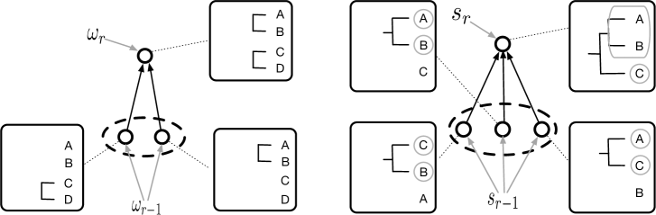
Figure 1: Illustration of the overcounting issues in (a) original CSMC. The partial state $(A,B),(C,D)$ can be constructed in two different ways: by first merging $A$ and $B$, then merging $C$ and $D$, or by first merging $C$ and $D$, then merging $A$ and $B$; (b) proposed CSMC. The augmented partial state $s_{r}$ can be constructed in three different ways. The two grey circles of each augmented partial state indicate the two subtrees that are just merged.

2 Background and notation

We denote our observed biological sequence data by $y$. Let $X$ be a set of observed taxa. A phylogenetic X-tree $t$ represents the relationship among observed taxa via a tree topology and a set of branch lengths. We only focus on the binary tree reconstruction. Let $\theta$ denote the parameter in a nucleotide substitution model. The prior distribution of $\theta$ and $t$ are denoted by $p(\theta)$ and $p(t|\theta)$ respectively. The likelihood of data $y$ given $t$ and $\theta$ is denoted by $p(y|t,\theta)$. The joint posterior of $t$ and $\theta$ is denoted by $\pi(t,\theta)$. We introduce the notation $\gamma(\cdot)$ to denote the unnormalized posterior density.

In Bayesian phylogenetics, our objective is to estimate the posterior distribution of $t$ and $\theta$,

$$\pi(\theta,t)=\frac{p(y|\theta,t)p(t|\theta)p(\theta)}{p(y)}.$$ (1)

Here $p(y)=\int\int p(y|\theta,t)p(t|\theta)p(\theta)\,\mathrm{d}\theta\,\mathrm{d}t$ is the marginal likelihood of biological sequence data.

With a site independence assumption, the likelihood function $p(y|\theta,t)$ can be evaluated by Felsenstein pruning (Felsenstein, 1973, 1981), which involves the calculation of the probability of nucleotide mutation given a fixed amount of evolution (i.e. the branch length). We use a continuous-time Markov chain (CTMC) to model the evolution of each site along each branch of $t$. There is rich literature about phylogenetic nucleotide substitution models, such as the Jukes-Cantor (JC) model (Jukes et al., 1969), the Kimura 2-parameter (K2P) model (Kimura, 1980), and the general time reversible (GTR) model (Rodriguez et al., 1990). The evolutionary model considered in this article is the K2P model. The rate matrix of the CTMC for K2P model only has one unknown parameter, $\kappa$, that represents the ratio of transition to transversion. In this case, the evolutionary model $\theta=\kappa$. See Supplementary Material Section 1 for details.

A common assumption in Bayesian phylogenetics is that the priors for $\theta$ and $t$ are independent, i.e. $p(t|\theta)=p(t)$. A common prior over non-clock trees consists of a uniform distribution on topologies and a product of independent exponential distributions with rate $\lambda$ on branch lengths. A commonly used prior for $\kappa$ in K2P model is an exponential distribution with rate $\mu_{0}$. We will use a coalescent tree prior for clock trees.

The exact evaluation of the normalized posterior $\pi(\theta,t)$ requires computing the marginal likelihood $p(y)$, which is generally intractable in phylogenetics. We review classical MCMC methods for Bayesian phylogenetic inference in Supplementary Material Section 2 and list all notations in Supplementary Material Table 2.

3 Phylogenetic tree inference

In this section, we assume that the parameter $\theta$ in the nucleotide substitution model is known. We are interested in the posterior inference over phylogenetic trees $\pi(t)$.

3.1 Combinatorial sequential Monte Carlo

Combinatorial sequential Monte Carlo (CSMC) (Wang et al., 2015) is an SMC algorithm for general tree inference based on a graded partially ordered set (poset) on an extended combinatorial space. The essential idea of the CSMC algorithm is to introduce a sequence of $R$ intermediate states to construct the target phylogenetic tree $t$ incrementally. These $R$ intermediate states are typically graded from ‘simple’ to ‘complex’. The CSMC algorithm sequentially approximates these intermediate distributions efficiently. The last intermediate distribution is the posterior of tree $\pi(t)$.

We use ${\color[rgb]{0,0,0}\omega}_{1},{\color[rgb]{0,0,0}\omega}_{2},\dots,{\color[rgb]{0,0,0}\omega}_{R}$ to denote the sequence of intermediate states. We call state ${\color[rgb]{0,0,0}\omega}_{r}$ a partial state of rank $r$. For example, a partial state of rank $r$ can be a phylogenetic forest over the observed taxa, defined as a set of $R-r+1$ phylogenetic trees. We use the notation ${\color[rgb]{0,0,0}\Omega}_{r}$ to denote the set of partial states of rank $r$, and define ${\color[rgb]{0,0,0}\Omega}=\bigcup{\color[rgb]{0,0,0}\Omega}_{r}$. We use the notation $|{\color[rgb]{0,0,0}\omega}|$ to denote the number of trees in a forest ${\color[rgb]{0,0,0}\omega}$. Recall that our interest is in inferring $\pi(t)$ with $\gamma(t)$. Here $\gamma(t)$ denotes an unnormalized $\pi(t)$. A natural extension from unnormalized posteriors on trees to the unnormalized posterior $\gamma$ on a forest is to take a product over the trees in the forest ${\color[rgb]{0,0,0}\omega}$ as follows:

$$\gamma({\color[rgb]{0,0,0}\omega})=\prod_{(t_{i},X_{i})\in{\color[rgb]{0,0,0}\omega}}\gamma_{y(X_{i})}(t_{i}),$$ (2)

where $t_{i}$ denotes one tree $i$ in forest ${\color[rgb]{0,0,0}\omega}$, $X_{i}$ denotes the taxa of $t_{i}$ and $y(X_{i})$ denotes the data associated with $X_{i}$.

CSMC algorithms iterate between resampling, propagation, and re-weighting to propose samples of rank $r$ from samples of rank $r-1$. We let ${\color[rgb]{0,0,0}\omega}_{r-1,k}$ denote the $k$-th particle of rank $r-1$. First, we resample $K$ times from the empirical posterior $\pi_{r-1}({\color[rgb]{0,0,0}\omega})=\sum_{k=1}^{K}W_{r-1,k}\delta_{{\color[rgb]{0,0,0}\omega}_{r-1,k}}({\color[rgb]{0,0,0}\omega})$, where $\delta$ is the delta function, and denote the particles after resampling by $\tilde{{\color[rgb]{0,0,0}\omega}}_{r-1,k}$, $k=1,2,\ldots,K$. Second, we use a proposal distribution $\nu_{\tilde{\color[rgb]{0,0,0}\omega}_{r-1,k}}^{+}(\cdot)$ to propose samples ${\color[rgb]{0,0,0}\omega}_{r,k}$ from $\tilde{\color[rgb]{0,0,0}\omega}_{r-1,k}$. Finally, we compute a weight update for each particle. Figure 1 (a) displays the overcounting issue for CSMC in non-clock tree inference. As shown in the figure, one intermediate state (${\color[rgb]{0,0,0}\omega}_{r}$) may have multiple ancestors (${\color[rgb]{0,0,0}\omega}_{r-1}$), which may lead to an inconsistent estimator if a standard SMC weight update is used. Instead, CSMC uses the following formula for the particle weight update:

$$w_{r,k} =\tilde{w}_{r-1,k}\cdot w(\tilde{\color[rgb]{0,0,0}\omega}_{r-1,k},{\color[rgb]{0,0,0}\omega}_{r,k}),$$ (3)

$$w(\tilde{\color[rgb]{0,0,0}\omega}_{r-1,k},{\color[rgb]{0,0,0}\omega}_{r,k}) =\frac{\gamma({\color[rgb]{0,0,0}\omega}_{r,k})}{\gamma(\tilde{\color[rgb]{0,0,0}\omega}_{r-1,k})}\cdot\frac{\nu_{{\color[rgb]{0,0,0}\omega}_{r,k}}^{-}(\tilde{\color[rgb]{0,0,0}\omega}_{r-1,k})}{\nu_{\tilde{\color[rgb]{0,0,0}\omega}_{r-1,k}}^{+}({\color[rgb]{0,0,0}\omega}_{r,k})},$$ (4)

where $\tilde{w}_{r-1,k}$ is the unnormalized particle weight from the previous iteration, $\nu^{-}$ is a backward kernel to correct an overcounting problem in non-clock tree inference and $\nu^{+}$ is the forward kernel that is the proposal in the second step. It is shown in Wang et al. (2015) that a CSMC with the weight update in (3) can provide a consistent estimate of the posterior distribution.

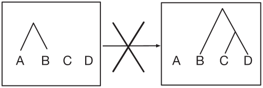
Figure 2: An example to illustrate the limitation of the merge proposal. If a clade (A, B) exists in the partial state $\tilde{{\color[rgb]{0,0,0}\omega}}_{r-1}$, we cannot propagate clade (B, (C, D)) in the partial state ${\color[rgb]{0,0,0}\omega}_{r}$ using this merge proposal distribution.

The efficiency of the CSMC depends on several factors, including the choice of proposal distributions and resampling schemes. This paper will only focus on the proposal distributions. If the proposal distribution is inefficient, the path degeneracy issue of SMC can become serious when it is combined with MCMC in the framework of particle Gibbs. A simple proposal is to propose new samples through randomly choosing a pair of subtrees to merge (i.e. picking a pair of trees in $\tilde{{\color[rgb]{0,0,0}\omega}}_{r-1}$ uniformly at random among the $\binom{|\tilde{{\color[rgb]{0,0,0}\omega}}_{r-1}|}{2}$ pairs) and sample new branch lengths. Note that these subtrees can also be singletons. We will call this proposal the merge proposal and denote $m^{+}_{{\color[rgb]{0,0,0}\omega}}({\color[rgb]{0,0,0}\omega}^{\prime})$ for the density of proposing ${\color[rgb]{0,0,0}\omega}^{\prime}$ from ${\color[rgb]{0,0,0}\omega}$. This proposal is easy to implement but has some constraints. Figure 2 shows an example illustrating this constraint. If a clade (A, B) exists in the partial state $\tilde{{\color[rgb]{0,0,0}\omega}}_{r-1}$, we cannot propagate samples of partial states ${\color[rgb]{0,0,0}\omega}_{r}$ without this clade. Consequently, we cannot propose $\{A,(B,(C,D))\}$ from $\{(A,B),C,D\}$. This motivates us to develop a novel proposal distribution that can improve the performance of CSMC and can be used in particle Gibbs methods.

3.2 CSMC with the RDouP proposal

We will improve the CSMC by constructing a novel and sophisticated proposal based on its current proposal distribution. To distinguish the two proposals and their corresponding CSMC algorithms, we will call the unimproved CSMC the vanilla CSMC and its proposal distribution a base propagation or base proposal. Our new proposal distribution is based on the base proposal and will be called the RDouP proposal, short for Revert-Double-BasePropagation, for a reason which is explained later in this section. Correspondingly, the CSMC with the RDouP proposal is named CSMC-RDouP.

The CSMC-RDouP algorithm will need a different sequence of intermediate states, denoted by $s_{1},s_{2},\ldots,s_{R}$. We call $s_{r}$ the $r$-th augmented (partial) state because it is based on the partial state in Section 3.1. Recall that a base partial state ${\color[rgb]{0,0,0}\omega}$ is a forest of trees with subtrees ${(t_{i},X_{i})\in{\color[rgb]{0,0,0}\omega}},i=1,\ldots,|{\color[rgb]{0,0,0}\omega}|$. We let an augmented partial state $s$ be composed of a base partial state ${\color[rgb]{0,0,0}\beta}(s)\in{\color[rgb]{0,0,0}\Omega}$ and some extra information related to the base proposal. With the merge base proposal, the extra information includes two trees that are children of one of the trees in ${\color[rgb]{0,0,0}\beta}(s)$.

In CSMC-RDouP, we introduce $R$ intermediate target distributions on the $R$ augmented states. For the $r$-th augmented state, $s_{r}$, we let $\gamma(s_{r})=\gamma({\color[rgb]{0,0,0}\beta}(s_{r}))$, which is the unnormalized posterior distribution for the forest ${\color[rgb]{0,0,0}\beta}(s_{r})$. And $s_{r}$ is of rank $r$, the same rank as ${\color[rgb]{0,0,0}\beta}(s_{r})$. We use $\mathcal{S}_{r}$ to denote the set of augmented partial state of rank $r$, and define $\mathcal{S}=\bigcup\mathcal{S}_{r}$.

Figure 3 presents an overview of the CSMC-RDouP algorithmic framework. The CSMC-RDouP algorithm sequentially approximates $\pi(s_{r})$ $(r=2,3,\ldots,R)$. The algorithm is initialized at rank $r=1$ by initializing the list with $K$ copies of the least partial state $s_{1}$ (a list of taxa without any connections among them) and an empty set of trees that are most recently merged with the same weight. Given a list of weighted particles of the partial state $s_{r-1}$, the CSMC-RDouP algorithm performs the following three steps to approximate $\pi(s_{r})$: resampling, propagation, and re-weighting.

Resampling: First, we conduct a resampling step to resample $K$ particles from the empirical distribution $\pi_{r-1}(s)=\sum_{k=1}^{K}W_{r-1,k}\delta_{s_{r-1,k}}(s)$ and denote the resampled particles by $\tilde{s}_{r-1,1}$, $\tilde{s}_{r-1,2}$, $\ldots$, $\tilde{s}_{r-1,K}$. The resampling step prunes particles with low weights. A list of equally weighted samples is obtained after performing the resampling step. Instead of conducting resampling at every SMC iteration, we resample particles in an adaptive fashion (Doucet and Johansen, 2011). We compute a measure of particle degeneracy at every iteration, and perform resampling only when the particle degeneracy exceeds a pre-determined threshold. Effective sample size (ESS) is the standard criteria for measuring the particle degeneracy. To make the algorithm more efficient, we only resample when the relative effective sample size (rESS) falls below a threshold. The relative effective sample size (rESS) is defined as s $\text{rESS}(W_{\cdot})=\bigg{(}K\sum_{k=1}^{K}W_{k}^{2}\bigg{)}^{-1}$, where $W_{\cdot}$ represents a vector of length $K$ for the normalized particle weights.

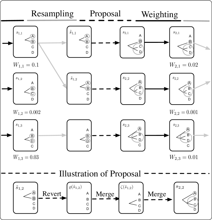
Figure 3: An overview of the CSMC-RDouP framework. A set of partial states is kept at each SMC iteration. A positive-valued weight is associated with each partial state. Given a list of weighted particles of the partial state $s_{r-1}$, the CSMC-RDouP algorithm performs the following three steps to approximate $\pi(s_{r})$: (i) resample to prune particles with small weights, (ii) propose a new partial state through the RDouP proposal, and (iii) compute the weights for new particles. The lower panel of the figure provides an example of the proposal. The two grey circles of each particle indicate the two subtrees that are just merged.

Propagation: Second, we propagate a new particle of rank $r$, denoted by $s_{r,k}$ from each of the resampled particle $\tilde{s}_{r-1,k}$ ($\tilde{s}_{r-1,k}=s_{r-1,k}$ if we do not conduct resampling at rank $r-1$), using a proposal distribution $\nu^{+}_{\tilde{s}_{r-1,k}}:\mathcal{S}\to[0,1]$.

We construct a sophisticated proposal based on a base proposal using three steps. The first step is to undo the last base proposal; the second step is to conduct one base proposal; and the third step is to do another base proposal and keep relevant information for undoing this move later. In other words, the new proposal is based on reverting the augmented partial state and then double implementing the base propagation, called Revert-Double-BasePropagation (RDouP) proposal.

To be more concrete, we will introduce some notation and use the merge proposal as an example of the base proposal. The reverted state of an augmented partial state, $s=\{{\color[rgb]{0,0,0}\omega},(t_{i},X_{i}),(t_{j},X_{j})\}$, is obtained by removing the tree with two children $(t_{i},X_{i})$ and $(t_{j},X_{j})$ from ${\color[rgb]{0,0,0}\omega}$, but keeping $(t_{i},X_{i})$ and $(t_{j},X_{j})$. That is,

$$\varrho(s)=\{{\color[rgb]{0,0,0}\omega}\backslash((t_{i},X_{i}),(t_{j},X_{j}))\}\cup\{(t_{i},X_{i}),(t_{j},X_{j})\},$$ (5)

where $((t_{i},X_{i}),(t_{j},X_{j}))$ is the clade with children $(t_{i},X_{i})$ and $(t_{j},X_{j})$. In contrast, we can reduce an augmented partial state to a base partial state

$${\color[rgb]{0,0,0}\beta}(s)={\color[rgb]{0,0,0}\omega}=s\backslash\{(t_{i},X_{i}),(t_{j},X_{j})\}.$$ (6)

The probability density of proposing a new state $s_{r,k}$ from the current state $\tilde{s}_{r-1,k}$ is denoted by $\nu^{+}_{\tilde{s}_{r-1,k}}(s_{r,k})$. There are 3 steps in propagating $s_{r,k}$:

1. Find the reverted base state of the current augmented partial state $\tilde{s}_{r-1,k}$, denoted by $\varrho(\tilde{s}_{r-1,k})$.

2. We first pick a pair of trees in $\varrho(\tilde{s}_{r-1,k})$ uniformly at random among the $\binom{|\varrho(\tilde{s}_{r-1,k})|}{2}$ pairs, and then sample the length of the new branches. This state is denoted by ${\color[rgb]{0,0,0}\zeta}(\tilde{s}_{r-1,k})$.

3. We pick a pair of trees in ${\color[rgb]{0,0,0}\zeta}(\tilde{s}_{r-1,k})$ uniformly at random among the $\binom{|{\color[rgb]{0,0,0}\zeta}(\tilde{s}_{r-1,k})|}{2}$ pairs, and sample the length of the new branches. We also keep the two trees that are merged together with the progagated partial state. This step finishes the propagation of $s_{r,k}$.

To ease the description of the algorithm, we call $\tilde{s}_{r-1,k}$ the parent state of $s_{r,k}$, and call $\varrho(\tilde{s}_{r-1,k})$ the reverted state of $\tilde{s}_{r-1,k}$. The lower panel of Figure 3 displays an example of proposing $s_{r,k}$ from $\tilde{s}_{r-1,k}$ using the RDouP proposal based on the merge proposal. In this example, we first find the reverted state of $\{(A,B),C,D),A,B\}$, which is $\{A,B,C,D\}$. Then we merge $B$ and $C$, and merge $(B,C)$ and $A$ to form the augmented partial state, $\{(A,(B,C)),D,A,(B,C)\}$. The parent state of $s_{r,k}$ is $\tilde{s}_{r-1,k}$, and its reverted state is ${\color[rgb]{0,0,0}\zeta}(\tilde{s}_{r-1,k})$. s

The forward kernel in CSMC-RDouP has the following form:

$$\nu_{\tilde{s}_{r-1,k}}^{+}(s_{r,k})=r_{\tilde{s}_{r-1,k}}^{+}({\varrho}(\tilde{s}_{r-1,k}))\cdot m_{{\varrho}(\tilde{s}_{r-1,k})}^{+}({\color[rgb]{0,0,0}\zeta}(\tilde{s}_{r-1,k}))\cdot{\color[rgb]{0,0,0}\check{m}}_{{\color[rgb]{0,0,0}\zeta}(\tilde{s}_{r-1,k})}^{+}({\color[rgb]{0,0,0}s_{r,k}}),$$ (7)

where $r^{+}_{s}({\color[rgb]{0,0,0}\omega})$ is 1 if ${\color[rgb]{0,0,0}\omega}$ is the reverted state of $s$, otherwise 0; $m^{+}_{{\color[rgb]{0,0,0}\omega}}({\color[rgb]{0,0,0}\omega}^{\prime})$ is the density of proposing a base state ${\color[rgb]{0,0,0}\omega}^{\prime}$ from a base state ${\color[rgb]{0,0,0}\omega}$; $\check{m}^{+}_{{\color[rgb]{0,0,0}\omega}}(s)$ is the density of proposing an augmented state $s$ from a base state ${\color[rgb]{0,0,0}\omega}$. Note that in $\check{m}_{{\color[rgb]{0,0,0}\omega}}^{+}(s)$, we propose an augmented state $s$ from a base state ${\color[rgb]{0,0,0}\omega}$ by keeping the two trees that are most recently merged; hence, $\check{m}^{+}_{{\color[rgb]{0,0,0}\omega}}(s)=m_{{\color[rgb]{0,0,0}\omega}}^{+}{(\beta(s))}$, where $\beta(s)$ is a base state reduced from the augmented state $s$.

Re-weighting: Finally, we compute a weight for each of these new particles using the same weight update formula in Equation (3) in the vanilla version of CSMC because the RDouP proposal also generates the overcounting issue. Figure 1 (b) illustrates the overcounting issue in CSMC-RDouP, where there are multiple ways to propose the same augmented partial state. Due to the overcounting issue, a backward kernel is required in the weight update to obtain a consistent estimate for the posterior distribution.

We propose to use the backward kernel as follows:

$$\nu_{s_{r,k}}^{-}(\tilde{s}_{r-1,k})$$ (8)

$$= m_{{\color[rgb]{0,0,0}\beta(s_{r,k})}}^{-}({\color[rgb]{0,0,0}\zeta}(\tilde{s}_{r-1,k}))\cdot m_{{\color[rgb]{0,0,0}\zeta}(\tilde{s}_{r-1,k})}^{-}(\varrho(\tilde{s}_{r-1,k}))\cdot r_{\varrho(\tilde{s}_{r-1,k})}^{-}(\tilde{s}_{r-1,k}),$$

where $m^{-}_{{\color[rgb]{0,0,0}\omega}}({\color[rgb]{0,0,0}\omega}^{\prime})>0$ if there are multiple ways proposing a base state ${\color[rgb]{0,0,0}\omega}^{\prime}$ from a base state ${\color[rgb]{0,0,0}\omega}$ using $m^{+}$, and $r^{-}_{{\color[rgb]{0,0,0}\omega}}(s)>0$ if ${\color[rgb]{0,0,0}\omega}$ is the reverted state of the augmented state $s$. We will show that this choice of backward kernel can lead to asymptotically consistent estimates in the Supplementary Material Section 3.

By plugging (7) and (8) into (4), the incremental weight function can be rewritten as

$$w(\tilde{s}_{r-1,k},s_{r,k})$$ (9)

$$= \frac{\gamma(s_{r,k})}{\gamma(\tilde{s}_{r-1,k})}\cdot\frac{m_{{\color[rgb]{0,0,0}\beta(s_{r,k})}}^{-}({\color[rgb]{0,0,0}\zeta}(\tilde{s}_{r-1,k}))\cdot m_{{\color[rgb]{0,0,0}\zeta}(\tilde{s}_{r-1,k})}^{-}(\varrho(\tilde{s}_{r-1,k}))\cdot r_{\varrho(\tilde{s}_{r-1,k})}^{-}(\tilde{s}_{r-1,k})}{r_{\tilde{s}_{r-1,k}}^{+}({\varrho}(\tilde{s}_{r-1,k}))\cdot m_{{\varrho}(\tilde{s}_{r-1,k})}^{+}({\color[rgb]{0,0,0}\zeta}(\tilde{s}_{r-1,k}))\cdot m_{{\color[rgb]{0,0,0}\zeta}(\tilde{s}_{r-1,k})}^{+}({\color[rgb]{0,0,0}\beta(s_{r,k})})}.$$

We construct a discrete positive measure using a list of weighted particles at rank $r$, $\pi_{r,K}(s)=\sum_{k=1}^{K}W_{r,k}\delta_{s_{r,k}}(s),\textrm{for all }s\in\mathcal{S}$. In the end, we obtain a Monte Carlo approximation $\pi_{R,K}$ of $\pi(t)$. Algorithm 1 summaries the CSMC-RDouP algorithm.

Algorithm 1 : RDouP combinatorial sequential Monte Carlo

1:Inputs: (a) Prior over augmented partial states $p(s)$; (b) Likelihood function $p(y|s,\theta)$; (c) Threshold of the rESS: $\epsilon$.

2:Outputs: Approximation of the posterior distribution, $\sum_{k}W_{R,k}\delta_{s_{R,k}}(\cdot)\approx\pi(\cdot)$.

3:Initialize SMC iteration index: $r\leftarrow 1$.

4:for $k\in\{1,\dots,K\}$ do

5:     Initialize particles with the least partial state.

6:     Initialize weights: $w_{1,k}\leftarrow 1$; $W_{1,k}\leftarrow 1/K$.

7:for  rank $r\in\{2,\dots,R\}$ do

8:     if $\text{rESS}(W_{r-1,\cdot})<\epsilon$ then

9:         Resample the particles.

10:         for $k\in\{1,\dots,K\}$ do

11:               Reset particle weights: $\tilde{w}_{r-1,k}=1$; $\tilde{W}_{r-1,k}=1/K$.          

12:     else

13:         for $k\in\{1,\dots,K\}$ do

14:              $\tilde{w}_{r-1,k}=w_{r-1,k};\tilde{s}_{r-1,k}=s_{r-1,k}$.               

15:     for  all $k\in\{1,\dots,K\}$ do

16:         Sample particles $s_{r,k}\sim\nu^{+}_{\tilde{s}_{r-1,k}}(\cdot)$, using one revert move to find $\varrho(\tilde{s}_{r-1,k})$, and two base proposals to propose ${\color[rgb]{0,0,0}\zeta}(\tilde{s}_{r-1,k})$ and $s_{r,k}$.

17:         Update weights according to Equation (3).      

Assumption 1.

For all $s$, $s^{\prime}\in\mathcal{S}$, $m^{+}_{s}(s^{\prime})=0$ implies $m^{-}_{s^{\prime}}(s)=0$.

Proposition 1.

For all $s$, $s^{\prime}\in\mathcal{S}$, if $m^{+}$ and $m^{-}$ satisfy Assumption 1, $\nu^{+}_{s}(s^{\prime})=0$ implies $\nu^{-}_{s^{\prime}}(s)=0$.

Proof.

We have $\nu_{s}^{+}(s^{\prime})=r^{+}_{s}(\varrho(s))\cdot m_{\varrho(s)}^{+}({\color[rgb]{0,0,0}\zeta}(s))\cdot m_{{\color[rgb]{0,0,0}\zeta}(s)}^{+}({\color[rgb]{0,0,0}\beta(s^{\prime})})$. Since $\varrho(s)$ is the reverted state of $s$, $r^{+}_{s}(\varrho(s))=1$. Hence $\nu_{s}^{+}(s^{\prime})=0$ implies that either $m_{\varrho(s)}^{+}({\color[rgb]{0,0,0}\zeta}(s))=0$ or $m_{{\color[rgb]{0,0,0}\zeta}(s)}^{+}({\color[rgb]{0,0,0}\beta(s^{\prime})})$ is 0.

Based on the Assumption 1 on the base proposal, $m_{\varrho(s)}^{+}({\color[rgb]{0,0,0}\zeta}(s))$ implies $m_{{\color[rgb]{0,0,0}\zeta}(s)}^{-}(\varrho(s))=0$, and $m_{{\color[rgb]{0,0,0}\zeta}(s)}^{+}({\color[rgb]{0,0,0}\beta}(s^{\prime}))$ implies $m_{{\color[rgb]{0,0,0}\beta}(s^{\prime})}^{-}({\color[rgb]{0,0,0}\zeta}(s))$=0. Hence, either $m_{{\color[rgb]{0,0,0}\zeta}(s)}^{-}(\varrho(s))=0$ or $m_{{\color[rgb]{0,0,0}\beta}(s^{\prime})}^{-}({\color[rgb]{0,0,0}\zeta}(s))=0$. Since $\nu_{s^{\prime}}^{-}(s)=m_{{\color[rgb]{0,0,0}\beta}(s^{\prime})}^{-}({\color[rgb]{0,0,0}\zeta}(s))\cdot m_{{\color[rgb]{0,0,0}\zeta}(s)}^{-}(\varrho(s))\cdot r^{-}_{\varrho(s)}(s)$, we have $\nu_{s^{\prime}}^{-}(s)=0$.

Proposition 2.

If for all $s$, $s^{\prime}\in\mathcal{S}$, $\nu^{+}_{s}(s^{\prime})=0$ implies $\nu^{-}_{s^{\prime}}(s)=0$, the CSMC-RDouP provides asymptotically consistent estimates. We have

$$\sum_{k=1}^{K}W_{R,k}\phi(s_{R,k})\to\int\pi_{R,k}(s)\phi(s)\text{d}s\leavevmode\nobreak\ \leavevmode\nobreak\ \text{as}\leavevmode\nobreak\ \leavevmode\nobreak\ K\to\infty,$$

where the convergence is in $L^{2}$ norm, and $\phi$ is a target function under mild conditions. For example, $\phi$ is a bounded function.

By construction, the RDouP proposal will induce a ranked poset defined on $\mathcal{S}$ such that $s^{\prime}$ covers $s$ if and only if $w(s,s^{\prime})>0$. In this poset structure, an augmented partial state $s$ is deemed to precede another augmented partial state $s^{\prime}$ if $s^{\prime}$ can be reached by obtaining the reverted state of $s$ followed by conducting two times of the base proposal and keeping the two trees that are merged in the second merge proposal. Consequently, the proposed CSMC-RDouP is within the framework of CSMC in Wang et al. (2015) and the consistency of posterior estimates is guaranteed by Proposition 2 in it. We refer readers to Wang et al. (2015) for the proof of consistency.

In the Supplementary Material Section 3, we explain the weight update for clock trees and non-clock trees in detail.

4 Joint estimation of phylogenetic tree and evolutionary parameter

4.1 Particle Gibbs Sampler

In a more realistic scenario, $\theta$ is also an unknown parameter that requires us to estimate given data. We study the particle Gibbs sampler, a Gibbs-type algorithm that iterates between sampling $t$ and $\theta$. Given a tree $t$, we use one Metropolis-Hastings step to sample $\theta$ from $\pi(\theta|t)$. Given $\theta$, a conditional CSMC-RDouP algorithm (described in Supplementary Material Section 4) is used to approximate $\pi(t|\theta)$. The main difference between the CSMC-RDouP algorithm and the conditional version is that in the latter, one of the particle trajectories is pre-specified, which is called the reference trajectory. This reference trajectory cannot be pruned in the resampling step. The resulting Markov chain of PGs will leave the target distribution invariant for an arbitrary number of particles used in the conditional CSMC-RDouP. Without loss of generality, we assume the first particle trajectory $s_{1:R,1}$ to be the reference trajectory, denoted by $s_{1:R}^{*}$. In PGs, we first use one Metropolis-Hastings step to update the parameter $\theta$, and then conditional on this $\theta$, we sample a particle trajectory from the approximated posterior of phylogenetic forests by running the conditional CSMC-RDouP. This sampled trajectory will be the reference trajectory of the conditional CSMC-RDouP in the next particle Gibbs iteration. We iterate these two steps until the convergence is achieved. We summarize the algorithm of PGs in the Supplementary Material Section 4.

4.2 Particle Gibbs Sampler with Ancestor Sampling

In particle Gibbs, the reference trajectory is kept intact throughout the CSMC-RDouP algorithm. This may lead to slow mixing of the PGs algorithm when path degeneracy exists. We investigate particle Gibbs with ancestor sampling (PGAs) (Lindsten et al., 2014) to improve the mixing of particle Gibbs samplers. The basic idea of PGAs is to include an ancestor sampling step in the conditional CSMC-RDouP algorithm to update the reference trajectory. If the reference trajectory is updated through the ancestor sampling step, the particle system may degenerate to a new trajectory other than the reference trajectory. We illustrate the implementation of the ancestor sampling step in the Supplementary Material Section 5.1.

4.3 Interacting particle Markov chain Monte Carlo

Another type of the particle Gibbs algorithm, interacting particle Markov chain Monte Carlo (IPMCMC) (Rainforth et al., 2016), is considered to improve the mixing of a particle Gibbs sampler. In IPMCMC, a pool of standard and conditional CSMC-RDouP algorithms are interacted to design an efficient proposal for tree posterior. The interaction of conditional and standard CSMC-RDouP algorithms is achieved by communicating their marginalized likelihoods. The algorithmic description of IPMCMC is displayed in the Supplementary Material Section 5.2. The standard and conditional CSMC-RDouP can be allocated into different computing cores to achieve parallelization.

5 Simulation studies

We assess the performance of the CSMC-RDouP method with simulation studies and provide main findings in this section. Please refer to Supplementary Material Section 6 for details.

We first emphasize a comparison of the vanilla CSMC and the proposed CSMC-RDouP in terms of computational speed. We find that the relative runtime of CSMC-RDouP compared with CSMC is about 1.4. The computational speed of CSMC-RDouP is lower than that of the vanilla CSMC. This is expected as the proposal in the vanilla CSMC is simpler, while in our new proposal we have to use one move to find the reverted state and merge twice to propose the new partial state. The weight update function in CSMC-RDouP algorithm is also more complicated.

We also compare the vanilla CSMC and the proposed CSMC-RDouP in terms of the tree reconstruction quality. The majority-rule consensus tree is used to summarize the weighted samples of phylogenetic trees (Felsenstein, 1981). We use the Robinson-Foulds (RF) metric based on sums of differences in branch lengths metric (Robinson and Foulds, 1979) to measure the distance between the estimated trees and true trees. From Figure 4, we conclude that the tree reconstruction accuracy increases with incremental numbers of particles. For larger trees, the reconstruction quality provided by the CSMC-RDouP is higher than the vanilla CSMC with a fixed computational budget, while the vanilla CSMC is better than CSMC-RDouP for trees with a small number of taxa.

We conducted another experiment to investigate the performance of the vanilla CSMC and CSMC-RDouP in PGs and IPMCMC, as a function of the number of particles. We also investigated the performance of PGAs with CSMC-RDouP. Figure 5 displays the comparison of PGs and IPMCMC with vanilla version of CSMC (IPGs, PGs) and CSMC-RDouP (IPGs-RDouP, PGs-RDouP) as a function of number of particles. For both PGs and IPMCMC with the vanilla CSMC, the log-likelihood of majority-rule consensus tree and RF metric do not improve if we increase $K$. PGs, IPMCMC, and PGAs with CSMC-RDouP perform better in terms of the log-likelihood and RF metric. If we increased $K$, the log-likelihoods increase and RF metrics decrease. The log-likelihood and RF metric provided by PGs, IPMCMC, and PGAs with CSMC-RDouP are close.

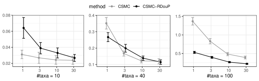
Figure 4: Comparison of CSMC and CSMC-RDouP as a function of number of (1000) particles in three scenarios: $10$ taxa (left), $40$ taxa (middle), $100$ taxa (right). The x-axis represents the number of a thousand particles. The four levels of $K$ (number of particles) from left to right of each panel for CSMC-RDouP are $1\cdot 10^{3}$, $3\cdot 10^{3}$, $1\cdot 10^{4}$ and $3\cdot 10^{4}$ respectively. The four levels of $K$ from left to right of each panel for vanilla version of CSMC are $1.5\cdot 10^{3}$, $4.5\cdot 10^{3}$, $1.5\cdot 10^{4}$, $4.5\cdot 10^{4}$ respectively. The y-axis represents the Robinson Foulds metric.

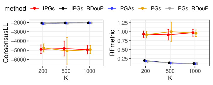
Figure 5: Comparison of PGs and IPMCMC with the vanilla CSMC (IPGs, PGs) and CSMC-RDouP (IPGs-RDouP, PGs-RDouP), PGAs with CSMC-RDouP (PGAs) as a function of number of particles. The x-axis represents number of particles. The three levels from left to right are $200$, $500$, $1000$, respectively. The y-axis of represents the log likelihood of the consensus tree and Robinson Foulds metric.

To understand the poor performance of the vanilla CSMC in the particle Gibbs samplers, we investigate the ESS in the conditional CSMC algorithm, which is the main component of particle Gibbs. Table 1 lists the mean ESS (0.025-quantile, 0.975-quantile) from all the iterations of the conditional CSMC algorithms using 100 runs of PGs, PGs-RDouP, PGAs-RDouP, respectively, for 3 scenarios. Although the mean ESS is generally larger in the vanilla conditional CSMC than that in the conditional CSMC-RDouP, there is a large percentage of cases in which the ESS is exactly equal to 1 (see the line with ‘ESS=1’ in Table 1), even when the number of taxa is as small as 7. Consequently, the Markov chain will get stuck at the same tree topology as the reference trajectory and hardly move. In contrast, all the ESS values are larger than 1 in both PGs-RDouP and PGAs-RDouP. The Markov chains are able to explore different tree topologies rather than the one on the reference trajectory.

Table 1: ESS (0.025-quantile, 0.975-quantile) in the conditional CSMC algorithms of PGs, PGs-RDouP, and PGAs-RDouP.

$\#$Taxa	$7$	$10$	$10$
Sequence length	$500$	$2000$	$2000$
$K$	$20000$	$10000$	$20000$
PGs	128 (1.000, 247)	21 (1.000, 85)	63 (1.000, 208)
ESS=1	0.6%	33.3%	11.1%
PGs-RDouP	112 (1.094, 520)	18 (1.011, 110)	42 (1.014, 295)
PGAs-RDouP	112 (1.953, 517)	19 (1.014, 110)	41 (1.043, 300)

We also find that, with a fixed computational cost, high values of $K$ are more important than the number of PGs iterations. In addition, the computing speed of CSMC-RDouP can increase notably from parallelization. See the Supplementary Material Section 6 for details.

6 Real data analysis

We analyze two real datasets of DNA sequences. We assume the K2P model for evolutionary process, and make the clock assumption for trees ($t$). We consider the inference of $t$ and $\theta$ via particle Gibbs sampler, and evaluate the tree construction quality using the log-likelihood function of majority-rule consensus tree.

The first real dataset we analyze is a set of DNA sequences for nine primates (Brown et al., 1982). In each DNA sequence, there are $888$ sites. As we have investigated in Simulation Studies, with a fixed computational budget, the number of particles ($K$) is more important than the number of MCMC iterations ($N$) in improving the mixing of algorithm. We fix the number of MCMC iterations $N=5000$, and vary $K$ to investigate the estimation by IPGs-RDouP and PGs. Table 2 displays the log-likelihood of the consensus tree provided by IPGs-RDouP and PGs with different number of particles. We select four levels of $K$ for PGs, $K=1000,2000,5000,10000$. We set the total number of nodes for running conditional CSMC and CSMC algorithms to be twice as the number of nodes running conditional CSMC ($M=2P$), and set $M=4$. We set $K$ for PGs $4$ times as large as each worker of IPMCMC, to guarantee fixed computational budgets for the two methods. For each algorithm, we repeat $10$ times.

Table 2 displays the log-likelihood (mean and standard deviation) of the consensus tree obtained from PGs and PGs-RDouP, with different numbers of particles; each case is repeated $10$ times with different initialization of evolutionary parameters and trees. The mixing of PG chains is poor even with $K=10000$. Multiple chains with different initializations do not converge to the same posterior distribution. The mixing of PGs-RDouP is improving when we increase the value of $K$. The log-likelihood gets higher and the standard deviation of log-likelihood decreases when we increase $K$. The PGs-RDouP chain mixes well when $K=10000$. Multiple chains with different initializations converge to the same posterior distribution. The mean and standard deviation for the posterior mean of $\theta$ for $10$ replications provided by PGs-RDouP are $3.68$ and $0.0094$, respectively. For one run of IPGs-RDouP, the posterior mean and $95\%$ credible interval of $\theta$ are $3.69$ and $(3.23,4.23)$ respectively.

In addition, we run PGs-RDouP and PGAs using $K=10000$ and $N=5000$. For comparison, we also run MrBayes for $5\cdot 10^{7}$ iterations. The log-likelihood of the consensus tree provided by MrBayes is $-5601.4$. The majority-rule consensus tree provided by IPGs-RDouP, PGs-RDouP, PGAs and MrBayes are the same, as displayed in Figure 6 of Supplementary Material Section 7.

The second real data analysis is presented in Supplementary Material Section 7.

Table 2: Log-likelihood of consensus trees provided by PGs and IPGs-RDouP, with mean (standard deviation), with varying numbers of particles.

$K$	$1000$	$2000$	$5000$	$10000$
PGs	-8424.1 (594.5)	-8247.0 (723.2)	-8333.8 (789.5)	-7930.9 (549.9)
IPGs-RDouP	-5626.8 (1.9)	-5611.4 (1.7)	-5580.6 (1.3)	-5553.8 (1.3)

7 Conclusion

We have proposed a combinatorial sequential Monte Carlo method with an RDouP proposal. Instead of randomly choosing a pair of trees to combine, we first use a revert step to find the reverted state of the current state, then in each merge step we randomly choose a pair of trees to combine. This proposal can benefit the exploration of tree posterior distribution. Our experimental results indicate that the RDouP proposal can improve the performance of CSMC, and this improvement can be enlarged when the number of taxa increases. The framework of CSMC-RDouP is also easy to parallelize. This makes the proposed CSMC more scalable to large DNA datasets compared with traditional Bayesian methods, such as MCMC.

Since SMC is a non-iterative algorithm, particles that fail to survive in the current iteration will not have a chance to come back to be part of the future enlarged particles. Consequently, path degeneracy is inevitable for SMC algorithms. This issue becomes more serious in conditional SMC algorithms. Therefore, methods that can mitigate the path degeneracy issue are crucial for improving the performance of SMC and the corresponding particle Gibbs samplers. Our proposed novel RDouP proposal provides a simple but effective way to reduce the path degeneracy issue for the combinatorial SMC algorithms. The idea is to allow one chance to regret the particle propagation by undoing the last propagation and then redoing the propagation twice. Note that although our method was motivated and illustrated using the phylogenetic applications, it can also be applied to other cases in which the CSMC is used. Also, the RDouP proposal can be based on other proposal distributions besides the simple merge proposal.

We have presented a particle Gibbs sampler, a hybrid of CSMC-RDouP and Gibbs sampler to estimate evolutionary parameters jointly with the phylogenetic trees. We have demonstrated the path degeneracy issue in the vanilla version of CSMC can be greatly mitigated in CSMC-RDouP. Consequently, CSMC-RDouP can be used in the particle Gibbs for phylogenetics, which previously suffers from the problem of poor mixing of the Markov chain. Moreover, CSMC-RDouP can be used in more advanced particle Gibbs samplers, including but not limited to particle Gibbs with ancestor sampling and interacting particle Markov chain Monte Carlo to achieve further improvements.

The consistency property of CSMC-RDouP holds when number of particles $K$ goes to infinity. However, $K$ cannot be made arbitrarily large in practice due to the memory limit. In addition, the computational costs of CSMC-RDouP increases linearly with number of particles $K$. A small value of $K$ may induce large bias for SMC estimates. Hence, it is important to select a proper value of $K$. Doucet et al. (2015) suggest selecting $K$ that the standard deviation of the log-likelihood estimate is around one so that the aysmptotic variance of the resulting PMCMC estimates is minimized with a fixed computational cost.

There are several possible directions to refine this methodology. First, we could explore more ways to allow the particles to undo the previous particle propagation. For example, we can use a different base proposal distribution, and we can revert the particles by undoing two steps of the base propagation. A second direction is to incorporate MCMC moves in CSMC-RDouP in a way that is described in Doucet and Johansen (2011) to further mitigate the path degeneracy issue by jittering the particles. Asymptotic variance of the SMC estimator was studied in Chopin (2004) under different resampling schemes, and displayed that advanced resampling schemes can reduce the variance of estimators. Another line of future work is to propose a computationally efficient resampling scheme, which is both unbiased and admits lower asymptotic variance for discrete tree spaces (Fearnhead and Clifford, 2003).

References

- Andrieu et al. (2010) Andrieu, C., Doucet, A., and Holenstein, R. (2010). Particle Markov chain Monte Carlo methods. Journal of the Royal Statistical Society B, 72(3), 269–342.
- Bouchard-Côté et al. (2012) Bouchard-Côté, A., Sankararaman, S., and Jordan, M. I. (2012). Phylogenetic inference via sequential Monte Carlo. Systematic Biology, 61, 579–593.
- Bouckaert et al. (2019) Bouckaert, R., Vaughan, T. G., Barido-Sottani, J., Duchêne, S., Fourment, M., Gavryushkina, A., Heled, J., Jones, G., Kühnert, D., De Maio, N., et al. (2019). BEAST 2.5: An advanced software platform for Bayesian evolutionary analysis. PLoS computational biology, 15(4), e1006650.
- Brown et al. (1982) Brown, W., Prager, E., Wang, A., and Wilson, A. (1982). Mitochondrial DNA sequences of primates: Tempo and mode of evolution. Journal of Molecular Evolution, 18(4), 225–239.
- Chopin (2004) Chopin, N. (2004). Central limit theorem for sequential Monte Carlo methods and its application to Bayesian inference. The Annals of Statistics, 32(6), 2385–2411.
- Del Moral et al. (2006) Del Moral, P., Doucet, A., and Jasra, A. (2006). Sequential Monte Carlo samplers. Journal of the Royal Statistical Society: Series B (Statistical Methodology), 68(3), 411–436.
- Dinh et al. (2017) Dinh, V., Darling, A. E., and Matsen IV, F. A. (2017). Online Bayesian phylogenetic inference: theoretical foundations via sequential Monte Carlo. Systematic biology, 67(3), 503–517.
- Doucet and Johansen (2011) Doucet, A. and Johansen, A. M. (2011). A tutorial on particle filtering and smoothing: fifteen years later. In Handbook of Nonlinear Filtering. Cambridge University Press.
- Doucet et al. (2001) Doucet, A., de Freitas, N., and Gordon, N. (2001). Sequential Monte Carlo methods in practice. Springer-Verlag, New York.
- Doucet et al. (2015) Doucet, A., Pitt, M. K., Deligiannidis, G., and Kohn, R. (2015). Efficient implementation of Markov chain Monte Carlo when using an unbiased likelihood estimator. Biometrika, 102(2), 295–313.
- Drummond and Suchard (2010) Drummond, A. and Suchard, M. (2010). Bayesian random local clocks, or one rate to rule them all. BMC biology, 8(1), 114.
- Everitt et al. (2020) Everitt, R. G., Culliford, R., Medina-Aguayo, F., and Wilson, D. J. (2020). Sequential Bayesian inference for mixture models and the coalescent using sequential Monte Carlo samplers with transformations. Statistics and Computing, 30(3), 663–676.
- Fearnhead and Clifford (2003) Fearnhead, P. and Clifford, P. (2003). On-line inference for hidden Markov models via particle filters. Journal of the Royal Statistical Society, Ser. B, 65, 887–899.
- Felsenstein (1973) Felsenstein, J. (1973). Maximum likelihood and minimum-steps methods for estimating evolutionary trees from data on discrete characters. Systematic Biology, 22(3), 240–249.
- Felsenstein (1981) Felsenstein, J. (1981). Evolutionary trees from DNA sequences: a maximum likelihood approach. Journal of molecular evolution, 17(6), 368–376.
- Fourment et al. (2017) Fourment, M., Claywell, B. C., Dinh, V., McCoy, C., Matsen, I., Frederick, A., and Darling, A. E. (2017). Effective online Bayesian phylogenetics via sequential Monte Carlo with guided proposals. Systematic biology.
- Görür and Teh (2009) Görür, D. and Teh, Y. W. (2009). An efficient sequential Monte Carlo algorithm for coalescent clustering. In Advances in Neural Information Processing Systems (NIPS).
- Görür et al. (2012) Görür, D., Boyles, L., and Welling, M. (2012). Scalable inference on Kingman’s coalescent using pair similarity. Journal of Machine Learning Research, 22, 440–448.
- Hajiaghayi et al. (2014) Hajiaghayi, M., Kirkpatrick, B., Wang, L., and Bouchard-Côté, A. (2014). Efficient continuous-time Markov chain estimation. In International Conference on Machine Learning (ICML), volume 31, pages 638–646.
- Huelsenbeck and Ronquist (2001) Huelsenbeck, J. P. and Ronquist, F. (2001). MRBAYES: Bayesian inference of phylogenetic trees. Bioinformatics, 17(8), 754–755.
- Jukes et al. (1969) Jukes, T. H., Cantor, C. R., et al. (1969). Evolution of protein molecules. Mammalian protein metabolism, 3(21), 132.
- Kimura (1980) Kimura, M. (1980). A simple method for estimating evolutionary rates of base substitutions through comparative studies of nucleotide sequences. Journal of molecular evolution, 16(2), 111–120.
- Lemey et al. (2009) Lemey, P., Rambaut, A., Drummond, A. J., and Suchard, M. A. (2009). Bayesian phylogeography finds its roots. PLoS Computational Biology, 5(9), e1000520.
- Lindsten et al. (2014) Lindsten, F., Jordan, M. I., and Schön, T. B. (2014). Particle Gibbs with ancestor sampling. The Journal of Machine Learning Research, 15(1), 2145–2184.
- Liu (2001) Liu, J. S. (2001). Monte Carlo Strategies in Scientific Computing. Springer.
- Rainforth et al. (2016) Rainforth, T., Naesseth, C., Lindsten, F., Paige, B., Vandemeent, J.-W., Doucet, A., and Wood, F. (2016). Interacting particle Markov chain Monte Carlo. In International Conference on Machine Learning, pages 2616–2625.
- Robinson and Foulds (1979) Robinson, D. F. and Foulds, L. R. (1979). Comparison of weighted labelled trees. In A. F. Horadam and W. D. Wallis, editors, Combinatorial Mathematics VI, pages 119–126, Berlin, Heidelberg. Springer Berlin Heidelberg.
- Rodriguez et al. (1990) Rodriguez, F., Oliver, J. L., Marin, A., and Medina, J. R. (1990). The general stochastic model of nucleotide substitution. Journal of theoretical biology, 142(4), 485–501.
- Ronquist and Huelsenbeck (2003) Ronquist, F. and Huelsenbeck, J. P. (2003). MrBayes 3: Bayesian phylogenetic inference under mixed models. Bioinformatics, 19(12), 1572–1574.
- Ronquist et al. (2012) Ronquist, F., Teslenko, M., van der Mark, P., Ayres, D. L., Darling, A., Hohna, S., Larget, B., Liu, L., Suchard, M. A., and Huelsenbeck, J. P. (2012). MrBayes 3.2: Efficient Bayesian phylogenetic inference and model choice across a large model space. Syst. Biol., 61, 539–542.
- Smith et al. (2017) Smith, R. A., Ionides, E. L., and King, A. A. (2017). Infectious disease dynamics inferred from genetic data via sequential Monte Carlo. Molecular biology and evolution, 34(8), 2065–2084.
- Suchard and Redelings (2006) Suchard, M. A. and Redelings, B. D. (2006). BAli-Phy: simultaneous Bayesian inference of alignment and phylogeny. Bioinformatics, 22(16), 2047–2048.
- Suchard et al. (2018) Suchard, M. A., Lemey, P., Baele, G., Ayres, D. L., Drummond, A. J., and Rambaut, A. (2018). Bayesian phylogenetic and phylodynamic data integration using BEAST 1.10. Virus evolution, 4(1), vey016.
- Teh et al. (2008) Teh, Y. W., Daumé III, H., and Roy, D. M. (2008). Bayesian agglomerative clustering with coalescents. In Advances in Neural Information Processing Systems (NIPS).
- Wang et al. (2015) Wang, L., Bouchard-Côté, A., and Doucet, A. (2015). Bayesian phylogenetic inference using a combinatorial sequential Monte Carlo method. Journal of the American Statistical Association, 110(512), 1362–1374.
- Wang et al. (2020) Wang, L., Wang, S., and Bouchard-Côté, A. (2020). An annealed sequential Monte Carlo method for Bayesian phylogenetics. Systematic Biology, 69(1), 155–183.