Hierarchical and Modularly-Minimal Vertex Colorings

Abstract

Cographs are exactly the hereditarily well-colored graphs, i.e., the graphs for which a greedy vertex coloring of every induced subgraph uses only the minimally necessary number of colors $\chi(G)$. We show that greedy colorings are a special case of the more general hierarchical vertex colorings, which recently were introduced in phylogenetic combinatorics. Replacing cotrees by modular decomposition trees generalizes the concept of hierarchical colorings to arbitrary graphs. We show that every graph has a modularly-minimal coloring $\sigma$ satisfying $|\sigma(M)|=\chi(M)$ for every strong module $M$ of $G$. This, in particular, shows that modularly-minimal colorings provide a useful device to design efficient coloring algorithms for certain hereditary graph classes. For cographs, the hierarchical colorings coincide with the modularly-minimal coloring. As a by-product, we obtain a simple linear-time algorithm to compute a modularly-minimal coloring of $P_{4}$-sparse graphs.

Keywords: proper vertex coloring; Grundy number; cographs; modular decomposition; chromatic number; $P_{4}$-sparse

1 Introduction

Graph coloring problems appear as a natural formalization of diverse real-life applications, describing in essence a partitioning of objects into classes under a given set of constraints [16, 18]. In this contribution, we investigate a specific type of vertex coloring that naturally appear in computational biology. A detailed knowledge of the evolutionary history of genes or species [6] is a prerequiste to answering many research questions in biology. In brief, the genome of an organism can be thought of as a collection of genes. All organisms that belong to the same species share the same collection of genes. Throughout evolution, species evolve independently of each other and occasionally subdivide to form new species. During this process of species-level evolution, also the genes within a species’ genomes change, and are sometimes lost or duplicated. Since only those genes residing in species that are alive at the present time can be observed and analyzed, the true evolutionary history cannot be observed directly and hence must be inferred, using algorithmic and statistical methods, from the genomic data available today. A question of considerable practical importance is to decide whether a pair of genes $x$ in species $A$ and $y$ in species $B$ are orthologs, i.e., originated in a speciation event, or paralogs, i.e., were produced by a gene duplication between speciation events [7, 26, 8]. Since the true history is unknown, orthologous gene pairs have to be distinguished from paralogs pairs using sequence similarity as a measure of evolutionary relatedness. A large class of methods to determine orthology starts from so-called pairwise best hits $\{x,y\}$, that is, of all genes in species $A$, the gene $x$ is most similar to $y$, and of all genes in $B$, $y$ is most similar to $x$ [1]. This defines a graph $G$ on the set of genes. A coloring $\sigma$ then assigns to each gene the species in which it resides. A key result of [10] is that if the edges of $G$ correctly represent orthology, then $(G,\sigma)$ is a so-called hierarchically-colored cograph (a restricted types of colorings in graphs that do not contain induced paths on four vertices). The requirement of an hierarchical coloring substantially strengthens the previously known necessary condition that $G$ must be a cograph [14].

In this contribution we first study the properties of hierarchical colorings and their relationship with greedy colorings of cographs. In particular, we show that a coloring of a cograph is a greedy coloring if and only if it is hierarchical w.r.t. all of its binary cotrees. On the other hand, a coloring is minimal on each intermediate step along a binary cotree if and only if it is hierarchical w.r.t. the same binary cotree. These results motivate concepts of hierarchical and modularly-minimal colorings of arbitrary graphs that are defined in terms of the modular decomposition. As a main result we show that every graph $G$ has a modularly-minimal coloring $\sigma$, that is, the subgraph $G[X]$ induced by any strong module $X$ of $G$ is minimally colored. As a by-product, we obtain a simple linear-time algorithm to compute a modularly-minimal coloring of $P_{4}$-sparse graphs in polynomial time.

2 Cographs and their Hierarchical Colorings

Let $G=(V,E)$ be an undirected graph. A (proper vertex) coloring of $G$ is a surjective map $\sigma:V\to S$ such that $xy\in E$ implies $\sigma(x)\neq\sigma(y)$. We will often refer to such coloring as an $|S|$-coloring. The minimum number $|S|$ of colors such that there is an $|S|$-coloring of $G$ is known as the chromatic number $\chi(G)$. For a subset $W\subseteq V$ (resp., a subgraph $H$ of $G$) we denote with $\sigma(W)$ (resp., $\sigma(H)$) the set of colors assigned to the vertices in $W$ (resp. $V(H)$) using $\sigma$.

A greedy coloring of $G$ is obtained by ordering the set of colors and coloring the vertices of $G$ in a random order with the first available color. The Grundy number $\gamma(G)$ is the maximum number of colors required in a greedy coloring of $G$ [4]. Obviously $\gamma(G)\geq\chi(G)$. Determining $\chi(G)$ [17] and $\gamma(G)$ [27] for arbitrary graphs are NP-complete problems. A graph $G$ is called well-colored if $\chi(G)=\gamma(G)$ [27]. It is hereditarily well-colorable if every induced subgraph is well-colorable. For later reference, we provide the following useful

Lemma 2.1.

Let $\sigma$ be a greedy coloring of a disconnected graph $G$ with connected components $G_{1},\dots,G_{k}$, $k\geq 2$ and let $H=\operatorname{\mathop{\vphantom{\bigcup}\mathchoice{\leavevmode\vtop{\halign{\hfil$\m@th\displaystyle#$\hfil\cr\bigcup\cr\cdot\crcr}}}{\leavevmode\vtop{\halign{\hfil$\m@th\textstyle#$\hfil\cr\bigcup\cr\cdot\crcr}}}{\leavevmode\vtop{\halign{\hfil$\m@th\scriptstyle#$\hfil\cr\bigcup\cr\cdot\crcr}}}{\leavevmode\vtop{\halign{\hfil$\m@th\scriptscriptstyle#$\hfil\cr\bigcup\cr\cdot\crcr}}}}\displaylimits}_{i\in I}G_{i}$ for some nonempty subset $I\subseteq\{1,\dots,k\}$. Then the restriction of $\sigma$ to $H$ is a greedy coloring of $H$.

Proof.

W.l.o.g. let the color set $\{1,\dots,|\sigma(G)|\}$ be naturally ordered from small to large integers. Since $\sigma$ is a greedy coloring it necessarily colors every connected component $G_{i}$ with colors $\{1,\dots,|\sigma(G_{i})|\}$. Moreover, let us preserve the ordering $\prec_{i}$ on the vertices in each $G_{i}$ according to the order they are visited during the greedy coloring in $G$. It is easy to verify that the first available color in $G$ to color a vertex $x$ in $G_{i}$ is precisely the first available to color $x$ when using the greedy coloring w.r.t. $\prec_{i}$ in $G_{i}$ only. In other words, the greedy coloring can be applied independently on the connected components, which completes the proof. ∎

Definition 2.1 ([5]).

A graph $G$ is a cograph if $G=K_{1}$, $G$ is the disjoint union $G=\operatorname{\mathop{\vphantom{\bigcup}\mathchoice{\leavevmode\vtop{\halign{\hfil$\m@th\displaystyle#$\hfil\cr\bigcup\cr\cdot\crcr}}}{\leavevmode\vtop{\halign{\hfil$\m@th\textstyle#$\hfil\cr\bigcup\cr\cdot\crcr}}}{\leavevmode\vtop{\halign{\hfil$\m@th\scriptstyle#$\hfil\cr\bigcup\cr\cdot\crcr}}}{\leavevmode\vtop{\halign{\hfil$\m@th\scriptscriptstyle#$\hfil\cr\bigcup\cr\cdot\crcr}}}}\displaylimits}_{i}G_{i}$ of cographs $G_{i}$, or $G$ is a join $G=\mathop{\vphantom{\sum}\mathchoice{\vbox{\hbox{\leavevmode\resizebox{9.00005pt}{}{$\triangledown$}}}}{\vbox{\hbox{\leavevmode\resizebox{10.00012pt}{}{$\triangledown$}}}}{\vbox{\hbox{\leavevmode\resizebox{7.00009pt}{}{$\triangledown$}}}}{\vbox{\hbox{\leavevmode\resizebox{5.00006pt}{}{$\triangledown$}}}}}\slimits@_{i}G_{i}$ of cographs $G_{i}$.

Since both operations, $\operatorname{\mathop{\vphantom{\bigcup}\mathchoice{\leavevmode\vtop{\halign{\hfil$\m@th\displaystyle#$\hfil\cr\bigcup\cr\cdot\crcr}}}{\leavevmode\vtop{\halign{\hfil$\m@th\textstyle#$\hfil\cr\bigcup\cr\cdot\crcr}}}{\leavevmode\vtop{\halign{\hfil$\m@th\scriptstyle#$\hfil\cr\bigcup\cr\cdot\crcr}}}{\leavevmode\vtop{\halign{\hfil$\m@th\scriptscriptstyle#$\hfil\cr\bigcup\cr\cdot\crcr}}}}\displaylimits}_{i}$ and $\mathop{\vphantom{\sum}\mathchoice{\vbox{\hbox{\leavevmode\resizebox{9.00005pt}{}{$\triangledown$}}}}{\vbox{\hbox{\leavevmode\resizebox{10.00012pt}{}{$\triangledown$}}}}{\vbox{\hbox{\leavevmode\resizebox{7.00009pt}{}{$\triangledown$}}}}{\vbox{\hbox{\leavevmode\resizebox{5.00006pt}{}{$\triangledown$}}}}}\slimits@_{i}$, are commutative and associative, each cograph can be written as the the join or disjoint union of two cographs. This recursive construction induces a rooted binary tree $T$, whose leaves are individual vertices corresponding to a $K_{1}$ and whose interior vertices correspond to the union and join operations. We write $L(T)$ for the leaf set and $V^{0}(T)\coloneqq V(T)\setminus L(T)$ for the set of inner vertices of $T$. The set of children of $u$ is denoted by $\mathsf{child}(u)$. For edges $e=uv$ in $T$ we adopt the convention that $v$ is a child of $u$. We define a labeling function $t:V^{0}(T)\rightarrow\{0,1\}$, where an interior vertex $u$ of $T$ is labeled $t(u)=0$ if it is associated with a disjoint union, and $t(u)=1$ for joins. We will refer to $(T,t)$ as a cotree. The tree $T(u)$ denotes the subtree of $T$ that is rooted at $u$. To simplify the notation we will write $G(u):=G[L(T(u))]$ for the subgraph of $G$ induced by the vertices in $L(T(u))$. Note that $G(u)$ is the graph consisting of the single vertex $u$ if $u$ is a leaf of $T$. Furthermore, $G(u)$ is a cograph by definition.

Given a cograph $G$, there is a unique discriminating cotree $(T^{*},t^{*})$ in which adjacent operations are distinct, i.e., $t^{*}(u)\neq t^{*}(v)$ for all interior edges $uv\in E(T)$. The discriminating cotree $(T^{*},t^{*})$ is obtained from every arbitrary binary cotree $(T,t)$ by contracting all edges $uv$ with $t(u)=t(v)$ into a single vertex $\overarc{uv}$ with label $t^{*}(\overarc{uv})=t(u)=t(v)$. Conversely, every binary cotree of $G$ can be obtained by replacing an inner vertex of $u$ and its children $u_{1},\dots,u_{k}$ by an arbitrary binary tree with root $u$, leaves $u_{1},\dots,u_{k}$ and all its inner vertices $w$ labeled by $t(w)=t^{*}(u)$, see e.g. [2, 5] for details.

It is possible to refine the discriminating cotree by subdividing a disjoint union or join into multiple disjoint unions or joins, respectively [2, 5]. It is well known that every induced subgraph of a cograph is again a cograph. A graph is a cograph if and only if it does not contain a path $P_{4}$ on four vertices as an induced subgraph [5]. The cographs are also exactly the hereditarily well-colored graphs [4]. The chromatic number of a cograph $G$ can be computed recursively, as observed in [5, Tab.1]. Starting from $\chi(K_{1})=1$ as base case we have

$$\begin{split}\chi(G)&=\chi\left(\operatorname{\mathop{\vphantom{\bigcup}\mathchoice{\leavevmode\vtop{\halign{\hfil$\m@th\displaystyle#$\hfil\cr\bigcup\cr\cdot\crcr}}}{\leavevmode\vtop{\halign{\hfil$\m@th\textstyle#$\hfil\cr\bigcup\cr\cdot\crcr}}}{\leavevmode\vtop{\halign{\hfil$\m@th\scriptstyle#$\hfil\cr\bigcup\cr\cdot\crcr}}}{\leavevmode\vtop{\halign{\hfil$\m@th\scriptscriptstyle#$\hfil\cr\bigcup\cr\cdot\crcr}}}}\displaylimits}_{i}G_{i}\right)=\max_{i}\chi(G_{i})\textrm{ or }\\ \chi(G)&=\chi\left(\mathop{\vphantom{\sum}\mathchoice{\vbox{\hbox{\leavevmode\resizebox{9.00005pt}{}{$\triangledown$}}}}{\vbox{\hbox{\leavevmode\resizebox{10.00012pt}{}{$\triangledown$}}}}{\vbox{\hbox{\leavevmode\resizebox{7.00009pt}{}{$\triangledown$}}}}{\vbox{\hbox{\leavevmode\resizebox{5.00006pt}{}{$\triangledown$}}}}}\slimits@_{i}G_{i}\right)=\sum_{i}\chi(G_{i})\end{split}$$ (1)

Hierarchically colored cographs (hc-cographs) were introduced in [10] as the undirected colored graphs recursively defined by

(K1)

$(G,\sigma)=(K_{1},\sigma)$, i.e., a colored vertex, or

(K2)

$(G,\sigma)=(H_{1},\sigma_{H_{1}})\operatorname{\triangledown}(H_{2},\sigma_{H_{2}})$ and $\sigma(V(H_{1}))\cap\sigma(V(H_{2}))=\emptyset$, or

(K3)

$(G,\sigma)=(H_{1},\sigma_{H_{1}})\mathbin{\mathchoice{\leavevmode\vtop{\halign{\hfil$\m@th\displaystyle#$\hfil\cr\cup\cr\cdot\crcr}}}{\leavevmode\vtop{\halign{\hfil$\m@th\textstyle#$\hfil\cr\cup\cr\cdot\crcr}}}{\leavevmode\vtop{\halign{\hfil$\m@th\scriptstyle#$\hfil\cr\cup\cr\cdot\crcr}}}{\leavevmode\vtop{\halign{\hfil$\m@th\scriptscriptstyle#$\hfil\cr\cup\cr\cdot\crcr}}}}(H_{2},\sigma_{H_{2}})$ and $\sigma(V(H_{1}))\cap\sigma(V(H_{2}))\in\{\sigma(V(H_{1})),\sigma(V(H_{2}))\}$,

where $\sigma(x)=\sigma_{H_{i}}(x)$ for every $x\in V(H_{i})$, $i\in\{1,2\}$ and $(H_{1},\sigma_{H_{1}})$ and $(H_{2},\sigma_{H_{2}})$ are hc-cographs.

Obviously, the graph $G$ underlying an hc-cograph is a cograph. Thus, the recursive construction of an hc-cograph $G$ implies a binary cotree $(T,t)$ that can be constructed with a top down approach as follows: Denote the root of $(T,t)$ by $r$. It is associated with the graph $G(r)=G$. In the general step we consider an induced subgraph $G(u)$ of $G$ associated with a vertex $u$ of $T$. If $G(u)$ is connected, then $t(u)=1$ and $G(u)$ is the joint of pair of induced subgraphs $G(v_{1})$ and $G(v_{2})$. To identify these graphs, consider the connected components $\overline{G_{1}},\dots,\overline{G_{k}}$ of the complement $\overline{G(u)}$ of $G(u)$. We have

$$G(u)=\overline{\operatorname{\mathop{\vphantom{\bigcup}\mathchoice{\leavevmode\vtop{\halign{\hfil$\m@th\displaystyle#$\hfil\cr\bigcup\cr\cdot\crcr}}}{\leavevmode\vtop{\halign{\hfil$\m@th\textstyle#$\hfil\cr\bigcup\cr\cdot\crcr}}}{\leavevmode\vtop{\halign{\hfil$\m@th\scriptstyle#$\hfil\cr\bigcup\cr\cdot\crcr}}}{\leavevmode\vtop{\halign{\hfil$\m@th\scriptscriptstyle#$\hfil\cr\bigcup\cr\cdot\crcr}}}}\displaylimits}_{i=1}^{k}\overline{G_{i}}}=\mathop{\vphantom{\sum}\mathchoice{\vbox{\hbox{\leavevmode\resizebox{9.00005pt}{}{$\triangledown$}}}}{\vbox{\hbox{\leavevmode\resizebox{10.00012pt}{}{$\triangledown$}}}}{\vbox{\hbox{\leavevmode\resizebox{7.00009pt}{}{$\triangledown$}}}}{\vbox{\hbox{\leavevmode\resizebox{5.00006pt}{}{$\triangledown$}}}}}\slimits@_{i=1}^{k}\overline{\overline{G_{i}}}=\mathop{\vphantom{\sum}\mathchoice{\vbox{\hbox{\leavevmode\resizebox{9.00005pt}{}{$\triangledown$}}}}{\vbox{\hbox{\leavevmode\resizebox{10.00012pt}{}{$\triangledown$}}}}{\vbox{\hbox{\leavevmode\resizebox{7.00009pt}{}{$\triangledown$}}}}{\vbox{\hbox{\leavevmode\resizebox{5.00006pt}{}{$\triangledown$}}}}}\slimits@_{i=1}^{k}G_{i}\,.$$ (2)

We therefore set $G(v_{1})=G_{1}$ and $G(v_{2})=\overline{\operatorname{\mathop{\vphantom{\bigcup}\mathchoice{\leavevmode\vtop{\halign{\hfil$\m@th\displaystyle#$\hfil\cr\bigcup\cr\cdot\crcr}}}{\leavevmode\vtop{\halign{\hfil$\m@th\textstyle#$\hfil\cr\bigcup\cr\cdot\crcr}}}{\leavevmode\vtop{\halign{\hfil$\m@th\scriptstyle#$\hfil\cr\bigcup\cr\cdot\crcr}}}{\leavevmode\vtop{\halign{\hfil$\m@th\scriptscriptstyle#$\hfil\cr\bigcup\cr\cdot\crcr}}}}\displaylimits}_{i=2}^{k}\overline{G_{i}}}=\mathop{\vphantom{\sum}\mathchoice{\vbox{\hbox{\leavevmode\resizebox{9.00005pt}{}{$\triangledown$}}}}{\vbox{\hbox{\leavevmode\resizebox{10.00012pt}{}{$\triangledown$}}}}{\vbox{\hbox{\leavevmode\resizebox{7.00009pt}{}{$\triangledown$}}}}{\vbox{\hbox{\leavevmode\resizebox{5.00006pt}{}{$\triangledown$}}}}}\slimits@_{i=2}^{k}G_{i}$. By construction, we therefore have $G(u)=G(v_{1})\operatorname{\triangledown}G(v_{2})$ with disjoint color sets $\sigma(G(v_{1}))$ and $\sigma(G(v_{2}))$. If $G(u)$ is disconnected, define $t(u)=0$, identify one of the components, say $G_{1}$, with the smallest numbers of colors $|\sigma(G_{1})|$ and set $G(v_{1})=G_{1}$ and $G(v_{2})=G(u)\setminus G(v_{1})$. The fact that $G(u)$ is an hc-cograph ensures that $\sigma(G(v_{1}))\subseteq\sigma(G(v_{2}))$. In both the connected and the disconnected case we attach $v_{1}$ and $v_{2}$ as the children of $u$ in $T$. The reconstruction of $(T,t)$ can be performed in linear time.

Definition 2.2.

A coloring $\sigma$ of a cograph $G$ is a hierarchical coloring w.r.t. the binary cotree $(T,t)$ if $(T,t)$ is a cotree of $G$ and $(G,\sigma)$ is a hc-cograph recursively constructed according to $(T,t)$.

As noticed in [10], a coloring $\sigma$ of a cograph $G$ may be hierarchical w.r.t. a binary cotree $(T,t)$ but not hierarchical w.r.t. another binary cotree $(T^{\prime},t^{\prime})$ that yields the same cograph. An example is shown in Fig. 1.

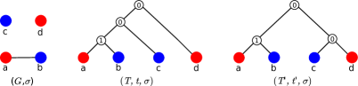
Figure 1: The induced cotree of a cograph $G$ affects the hierarchical coloring property of $\sigma$, where $\sigma(a)=\sigma(d)\neq\sigma(b)=\sigma(c)$. In $(T,t)$, the first tree from left to right, (K1)-(K3) are satisfied making $\sigma$ hierarchical. However the second tree $(T^{\prime},t^{\prime})$ does not satisfy (K3) since the parent node of $c\simeq K_{1}$ and $d\simeq K_{1}$ corresponds to a disjoint union operation and $\sigma(c)\cap\sigma(d)=\emptyset$. Thus $\sigma$ is not hierarchical w.r.t. $(T^{\prime},t^{\prime})$.

Every hierarchical coloring of a cograph is also a proper coloring (cf. [10, Lemma 43]). The property of being a cograph is hereditary (i.e., every induced subgraph of a cograph is a cograph). However, this is not necessarily true for hc-cographs. As an example consider the induced disconnected subgraph with vertices $c$ and $d$ of the hc-cograph in Fig. 1 that violates (K3). Nevertheless, if $G$ is an hc-cograph, then each of its connected components must be an hc-cograph (cf. [10, Lemma 44]). We show now that hc-cographs are always optimally colored.

Theorem 2.2.

Let $\sigma$ be a hierarchical coloring of a cograph $G$ w.r.t. some binary cotree $(T,t)$. Then $|\sigma(V)|=\chi(G)$.

Proof.

We proceed by induction w.r.t. $|V|$. The statement is trivially true for $|V|=1$, i.e. $G=K_{1}$, since $\chi(K_{1})=1$. Now suppose $|V|>1$. Thus, $G=G_{1}\operatorname{\triangledown}G_{2}$ or $G=G_{1}\mathbin{\mathchoice{\leavevmode\vtop{\halign{\hfil$\m@th\displaystyle#$\hfil\cr\cup\cr\cdot\crcr}}}{\leavevmode\vtop{\halign{\hfil$\m@th\textstyle#$\hfil\cr\cup\cr\cdot\crcr}}}{\leavevmode\vtop{\halign{\hfil$\m@th\scriptstyle#$\hfil\cr\cup\cr\cdot\crcr}}}{\leavevmode\vtop{\halign{\hfil$\m@th\scriptscriptstyle#$\hfil\cr\cup\cr\cdot\crcr}}}}G_{2}$ for some hc-cographs $G_{1}=(V_{1},E_{1})$ and $G_{1}=(V_{2},E_{2})$ with $1\leq|V_{1}|,|V_{2}|<|V|$. By induction hypothesis we have $|\sigma(V_{1})|=\chi(G_{1})$ and $|\sigma(V_{2})|=\chi(G_{2})$.

First consider $G=G_{1}\operatorname{\triangledown}G_{2}$. Since $xy\in E(G)$ for all $x\in V_{1}$ and $y\in V_{2}$ we have $\sigma(x)\neq\sigma(y)$, and hence $\sigma(V_{1})\cap\sigma(V_{2})=\emptyset$. Thus, $\sigma(V)=\sigma(V_{1})\mathbin{\mathchoice{\leavevmode\vtop{\halign{\hfil$\m@th\displaystyle#$\hfil\cr\cup\cr\cdot\crcr}}}{\leavevmode\vtop{\halign{\hfil$\m@th\textstyle#$\hfil\cr\cup\cr\cdot\crcr}}}{\leavevmode\vtop{\halign{\hfil$\m@th\scriptstyle#$\hfil\cr\cup\cr\cdot\crcr}}}{\leavevmode\vtop{\halign{\hfil$\m@th\scriptscriptstyle#$\hfil\cr\cup\cr\cdot\crcr}}}}\sigma(V_{2})$ and therefore,

$$|\sigma(V)|=|\sigma(V_{1})|+|\sigma(V_{2})|\stackrel{{\scriptstyle\text{IH.}}}{{=}}\chi(G_{1})+\chi(G_{2})\stackrel{{\scriptstyle\text{Equ.\ }\eqref{eq:rec1}}}{{=}}\chi(G).$$

We note that the coloring condition in (K2) therefore only enforces that $\sigma$ is a proper vertex coloring.

Now suppose $G=G_{1}\mathbin{\mathchoice{\leavevmode\vtop{\halign{\hfil$\m@th\displaystyle#$\hfil\cr\cup\cr\cdot\crcr}}}{\leavevmode\vtop{\halign{\hfil$\m@th\textstyle#$\hfil\cr\cup\cr\cdot\crcr}}}{\leavevmode\vtop{\halign{\hfil$\m@th\scriptstyle#$\hfil\cr\cup\cr\cdot\crcr}}}{\leavevmode\vtop{\halign{\hfil$\m@th\scriptscriptstyle#$\hfil\cr\cup\cr\cdot\crcr}}}}G_{2}$. Axiom (K3) implies $|\sigma(V)|=\max(|\sigma(V_{1})|,|\sigma(V_{2})|)$. Hence,

$$|\sigma(V)|=\max(|\sigma(V_{1})|,|\sigma(V_{2})|)\stackrel{{\scriptstyle\text{IH.}}}{{=}}\max(\chi(G_{1}),\chi(G_{2}))\stackrel{{\scriptstyle\text{Equ.\ }\eqref{eq:rec1}}}{{=}}\chi(G).$$

∎

Since the connected components of hc-cographs are again hc-cographs, the following statement is an immediate consequence of the recursive construction of hc-cographs:

Corollary 2.3.

If $\sigma$ is a hierarchical coloring of $G$ w.r.t. the binary cotree $(T,t)$, then $|\sigma(G(u))|=\chi(G(u))$ for all nodes $u$ of $(T,t)$ and $|\sigma(G^{\prime})|=\chi(G^{\prime})$ for all connected components $G^{\prime}$ of $G$.

As detailed in [4], we have $\chi(G)=\gamma(G)$ for cographs. Thus, it seems natural to ask whether every greedy coloring is hierarchical w.r.t. some binary cotree $(T,t)$. Making use of the fact that $\chi(G)=\gamma(G)$, we assume w.l.o.g. that the color set is $S=\{1,2,\dots,\chi(G)\}$ whenever we consider greedy colorings of a cograph.

We shall say that a cograph $G$ is a minimal counterexample for some property $\mathcal{P}$ if (1) $G$ does not satisfy $\mathcal{P}$ and (2) every induced subgraph of $G$ (i.e., every “smaller” cograph) satisfies $\mathcal{P}$.

Lemma 2.4.

Let $G$ be a cograph, $(T,t)$ an arbitrary binary cotree for $G$ and $\sigma$ a greedy coloring of $G$. Then $\sigma$ is a hierarchical coloring w.r.t. $(T,t)$.

Proof.

Assume $G$ is a minimal counterexample, i.e., $G$ is a minimal cograph for which a coloring $\sigma$ exists that is a greedy coloring but not an hierarchical coloring. If $G$ is connected, then either $G\simeq K_{1}$ or $G=\mathop{\vphantom{\sum}\mathchoice{\vbox{\hbox{\leavevmode\resizebox{9.00005pt}{}{$\triangledown$}}}}{\vbox{\hbox{\leavevmode\resizebox{10.00012pt}{}{$\triangledown$}}}}{\vbox{\hbox{\leavevmode\resizebox{7.00009pt}{}{$\triangledown$}}}}{\vbox{\hbox{\leavevmode\resizebox{5.00006pt}{}{$\triangledown$}}}}}\slimits@_{i=1}^{n}G_{i}$ and $\sigma(V)=\operatorname{\mathop{\vphantom{\bigcup}\mathchoice{\leavevmode\vtop{\halign{\hfil$\m@th\displaystyle#$\hfil\cr\bigcup\cr\cdot\crcr}}}{\leavevmode\vtop{\halign{\hfil$\m@th\textstyle#$\hfil\cr\bigcup\cr\cdot\crcr}}}{\leavevmode\vtop{\halign{\hfil$\m@th\scriptstyle#$\hfil\cr\bigcup\cr\cdot\crcr}}}{\leavevmode\vtop{\halign{\hfil$\m@th\scriptscriptstyle#$\hfil\cr\bigcup\cr\cdot\crcr}}}}\displaylimits}_{i=1}^{n}\sigma(V_{i})$ for some $n>1$, i.e., (K1) or (K2) is satisfied. By assumption, $\sigma$ is not a hierarchical coloring, hence $\sigma$ must fail to be a hierarchical coloring on at least one of the subgraphs $G_{i}$, contradicting the assumption that $G$ is a minimal counterexample. Thus, $G$ cannot be connected.

Therefore, assume that $G=\operatorname{\mathop{\vphantom{\bigcup}\mathchoice{\leavevmode\vtop{\halign{\hfil$\m@th\displaystyle#$\hfil\cr\bigcup\cr\cdot\crcr}}}{\leavevmode\vtop{\halign{\hfil$\m@th\textstyle#$\hfil\cr\bigcup\cr\cdot\crcr}}}{\leavevmode\vtop{\halign{\hfil$\m@th\scriptstyle#$\hfil\cr\bigcup\cr\cdot\crcr}}}{\leavevmode\vtop{\halign{\hfil$\m@th\scriptscriptstyle#$\hfil\cr\bigcup\cr\cdot\crcr}}}}\displaylimits}_{i=1}^{n}G_{i}$ for some $n>1$. Since $G$ is represented by a binary cotree $(T,t)$, the root of $T$ must have exactly two children $u$ and $v$. Hence, we can write $G=G(u)\mathbin{\mathchoice{\leavevmode\vtop{\halign{\hfil$\m@th\displaystyle#$\hfil\cr\cup\cr\cdot\crcr}}}{\leavevmode\vtop{\halign{\hfil$\m@th\textstyle#$\hfil\cr\cup\cr\cdot\crcr}}}{\leavevmode\vtop{\halign{\hfil$\m@th\scriptstyle#$\hfil\cr\cup\cr\cdot\crcr}}}{\leavevmode\vtop{\halign{\hfil$\m@th\scriptscriptstyle#$\hfil\cr\cup\cr\cdot\crcr}}}}G(v)$. Since $G$ is a minimal counterexample and since, by Lemma 2.1, $\sigma$ restricted to $G(u)$, resp., $G(v)$ is a greedy coloring of $G(u)$, resp., $G(v)$, we can conclude that $\sigma$ induces a hierarchical coloring on $G(u)$ and $G(v)$. However, since $\sigma$ is, in particular, a greedy coloring of $G(u)$ and $G(v)$, $\sigma(V(G(u)))\subseteq\sigma(V(G(v)))$ or $\sigma(V(G(v)))\subseteq\sigma(V(G(u)))$ most hold. But this immediately implies that $(G,\sigma)$ satisfies (K3) and thus $\sigma$ is a hierarchical coloring of $G$. Therefore, $G$ is not a minimal counterexample, which completes the proof. ∎

Since every cograph is well-colorable we obtain as an immediate consequence

Corollary 2.5.

Every cograph has a hierarchical coloring w.r.t. each of its binary cotrees $(T,t)$.

The converse of Lemma 2.4 is not true. Fig. 2 shows an example of a hierarchical coloring that is not a greedy coloring.

Figure 2: Both colorings A and B of $K_{2}\mathbin{\mathchoice{\leavevmode\vtop{\halign{\hfil$\m@th\displaystyle#$\hfil\cr\cup\cr\cdot\crcr}}}{\leavevmode\vtop{\halign{\hfil$\m@th\textstyle#$\hfil\cr\cup\cr\cdot\crcr}}}{\leavevmode\vtop{\halign{\hfil$\m@th\scriptstyle#$\hfil\cr\cup\cr\cdot\crcr}}}{\leavevmode\vtop{\halign{\hfil$\m@th\scriptscriptstyle#$\hfil\cr\cup\cr\cdot\crcr}}}}K_{1}\mathbin{\mathchoice{\leavevmode\vtop{\halign{\hfil$\m@th\displaystyle#$\hfil\cr\cup\cr\cdot\crcr}}}{\leavevmode\vtop{\halign{\hfil$\m@th\textstyle#$\hfil\cr\cup\cr\cdot\crcr}}}{\leavevmode\vtop{\halign{\hfil$\m@th\scriptstyle#$\hfil\cr\cup\cr\cdot\crcr}}}{\leavevmode\vtop{\halign{\hfil$\m@th\scriptscriptstyle#$\hfil\cr\cup\cr\cdot\crcr}}}}K_{1}$ are hierarchical colorings w.r.t. some cotrees. To see this, note that the coloring A is produced by $(K_{1}\operatorname{\triangledown}K_{1})\mathbin{\mathchoice{\leavevmode\vtop{\halign{\hfil$\m@th\displaystyle#$\hfil\cr\cup\cr\cdot\crcr}}}{\leavevmode\vtop{\halign{\hfil$\m@th\textstyle#$\hfil\cr\cup\cr\cdot\crcr}}}{\leavevmode\vtop{\halign{\hfil$\m@th\scriptstyle#$\hfil\cr\cup\cr\cdot\crcr}}}{\leavevmode\vtop{\halign{\hfil$\m@th\scriptscriptstyle#$\hfil\cr\cup\cr\cdot\crcr}}}}(K_{1}\mathbin{\mathchoice{\leavevmode\vtop{\halign{\hfil$\m@th\displaystyle#$\hfil\cr\cup\cr\cdot\crcr}}}{\leavevmode\vtop{\halign{\hfil$\m@th\textstyle#$\hfil\cr\cup\cr\cdot\crcr}}}{\leavevmode\vtop{\halign{\hfil$\m@th\scriptstyle#$\hfil\cr\cup\cr\cdot\crcr}}}{\leavevmode\vtop{\halign{\hfil$\m@th\scriptscriptstyle#$\hfil\cr\cup\cr\cdot\crcr}}}}K_{1})$, while coloring B is the result of $((K_{1}\operatorname{\triangledown}K_{1})\mathbin{\mathchoice{\leavevmode\vtop{\halign{\hfil$\m@th\displaystyle#$\hfil\cr\cup\cr\cdot\crcr}}}{\leavevmode\vtop{\halign{\hfil$\m@th\textstyle#$\hfil\cr\cup\cr\cdot\crcr}}}{\leavevmode\vtop{\halign{\hfil$\m@th\scriptstyle#$\hfil\cr\cup\cr\cdot\crcr}}}{\leavevmode\vtop{\halign{\hfil$\m@th\scriptscriptstyle#$\hfil\cr\cup\cr\cdot\crcr}}}}K_{1})\mathbin{\mathchoice{\leavevmode\vtop{\halign{\hfil$\m@th\displaystyle#$\hfil\cr\cup\cr\cdot\crcr}}}{\leavevmode\vtop{\halign{\hfil$\m@th\textstyle#$\hfil\cr\cup\cr\cdot\crcr}}}{\leavevmode\vtop{\halign{\hfil$\m@th\scriptstyle#$\hfil\cr\cup\cr\cdot\crcr}}}{\leavevmode\vtop{\halign{\hfil$\m@th\scriptscriptstyle#$\hfil\cr\cup\cr\cdot\crcr}}}}K_{1}$. Only A is a greedy coloring. The coloring B uses different colors for the two single-vertex components and thus is not greedy.

Theorem 2.6.

A coloring $\sigma$ of a cograph $G$ is a greedy coloring if and only if it is a hierarchical coloring w.r.t. every binary cotree $(T,t)$ of $G$.

Proof.

By Lemma 2.4, every greedy coloring is a hierarchical coloring for every binary cotree $(T,t)$. Now suppose $\sigma$ is an hierarchical coloring for every binary cotree $(T,t)$ and let $G$ be a minimal cograph for which $\sigma$ is not a greedy coloring. As in the proof of Lemma 2.4, we can argue that $G$ cannot be a minimal counterexample if $G$ is connected: in this case, $G=\mathop{\vphantom{\sum}\mathchoice{\vbox{\hbox{\leavevmode\resizebox{9.00005pt}{}{$\triangledown$}}}}{\vbox{\hbox{\leavevmode\resizebox{10.00012pt}{}{$\triangledown$}}}}{\vbox{\hbox{\leavevmode\resizebox{7.00009pt}{}{$\triangledown$}}}}{\vbox{\hbox{\leavevmode\resizebox{5.00006pt}{}{$\triangledown$}}}}}\slimits@_{i=1}^{n}G_{i}$ and $\sigma(V)=\operatorname{\mathop{\vphantom{\bigcup}\mathchoice{\leavevmode\vtop{\halign{\hfil$\m@th\displaystyle#$\hfil\cr\bigcup\cr\cdot\crcr}}}{\leavevmode\vtop{\halign{\hfil$\m@th\textstyle#$\hfil\cr\bigcup\cr\cdot\crcr}}}{\leavevmode\vtop{\halign{\hfil$\m@th\scriptstyle#$\hfil\cr\bigcup\cr\cdot\crcr}}}{\leavevmode\vtop{\halign{\hfil$\m@th\scriptscriptstyle#$\hfil\cr\bigcup\cr\cdot\crcr}}}}\displaylimits}_{i=1}^{n}\sigma(V_{i})$ for all colorings, and thus $\sigma$ is a greedy coloring if and only if it is a greedy coloring with disjoint color sets for each $G_{i}$. Hence, a minimal counterexample must have at least two connected components.

Let $G=\operatorname{\mathop{\vphantom{\bigcup}\mathchoice{\leavevmode\vtop{\halign{\hfil$\m@th\displaystyle#$\hfil\cr\bigcup\cr\cdot\crcr}}}{\leavevmode\vtop{\halign{\hfil$\m@th\textstyle#$\hfil\cr\bigcup\cr\cdot\crcr}}}{\leavevmode\vtop{\halign{\hfil$\m@th\scriptstyle#$\hfil\cr\bigcup\cr\cdot\crcr}}}{\leavevmode\vtop{\halign{\hfil$\m@th\scriptscriptstyle#$\hfil\cr\bigcup\cr\cdot\crcr}}}}\displaylimits}_{i=1}^{n}G_{i}$ for some $n>1$ and define a partition of $\{1,\dots,n\}$ into sets $I_{1},\dots,I_{\ell}$, $\ell\geq 1$, such that for every $r\in\{1,\dots,\ell\}$ we have $i,j\in I_{r}$ if and only if $\chi(G_{i})=\chi(G_{j})$. Since every $G^{r}\coloneqq\operatorname{\mathop{\vphantom{\bigcup}\mathchoice{\leavevmode\vtop{\halign{\hfil$\m@th\displaystyle#$\hfil\cr\bigcup\cr\cdot\crcr}}}{\leavevmode\vtop{\halign{\hfil$\m@th\textstyle#$\hfil\cr\bigcup\cr\cdot\crcr}}}{\leavevmode\vtop{\halign{\hfil$\m@th\scriptstyle#$\hfil\cr\bigcup\cr\cdot\crcr}}}{\leavevmode\vtop{\halign{\hfil$\m@th\scriptscriptstyle#$\hfil\cr\bigcup\cr\cdot\crcr}}}}\displaylimits}_{i\in I_{r}}G_{i}$, $1\leq r\leq\ell$, is a cograph, each $G^{r}$ can be represented by a (not necessarily unique) binary cotree $(T^{r},t^{r})$. Note, we have $\chi(G^{r})=\chi(G_{i})$ for all $i\in I_{r}$. Now, we can construct a binary cotree $(T,t)$ for $G$ as follows: let $T^{*}$ be a caterpillar with leaf set $L(T^{*})=\{l_{1},\dots,l_{\ell}\}$. We choose $T^{*}=(\ldots((l_{1},l_{2}),l_{3}),\ldots l_{\ell})$ (in Newick format). Note, if $\ell=1$, then $T^{*}\simeq K_{1}$. Now, the root of every tree $T^{1},\dots,T^{r}$ is identified with a unique leaf in $L(T^{*})$ such that the root of $T_{i}$ is identified with $l_{i}\in L(T^{*})$ and the root of $T_{j}$ is identified with $l_{j}\in L(T^{*})$, where $i<j$ if and only if $\chi(G^{i})<\chi(G^{j})$. This yields the tree $T$. The labeling $t$ for $(T,t)$ is provided by keeping the labels of each $(T^{r},t^{r})$ and by labeling all other inner vertices of $T$ by $0$. It is easy to see that $(T,t)$ is a binary cotree for $G$. By assumption, $\sigma$ is hierarchical w.r.t. $(T,t)$. We denote by $C(T^{*})\subseteq V(T)$ the set of inner vertices of $T^{*}$. Since $\sigma$ is hierarchical w.r.t. $(T,t)$ and thus in particular w.r.t. any subtree $(T^{r},t^{r})$, we have $\sigma(V(G_{i}))\cap\sigma(V(G_{j}))\in\{\sigma(V(G_{i})),\sigma(V(G_{j}))\}$ for any $i,j\in I_{r}$, $1\leq r\leq\ell$, by (K3). Hence, as $\chi(G^{r})=\chi(G_{i})=\chi(G_{j})$, it must necessarily hold $\sigma(V(G_{i}))=\sigma(V(G_{j}))$ for all $i,j\in I_{r}$, i.e., all connected components $G_{i}$ with the same chromatic number are colored by the same color set. By construction, at every node $v\in C(T^{*})$ of the caterpillar structure, with children $v^{\prime}$ and $v^{\prime\prime}$, the components $G^{\prime}:=G(v^{\prime})$ and $G^{\prime\prime}:=G(v^{\prime\prime})$ satisfy $\chi(G^{\prime})<\chi(G^{\prime\prime})$. Invoking (K3) we therefore have $\sigma(G^{\prime})\subset\sigma(G^{\prime\prime})$ and $G^{*}:=G(v)$ is colored by the color set $\sigma(G^{*})=\sigma(G^{\prime\prime})$. These set inclusions therefore imply a linear ordering of the colors such that colors in $\sigma(G^{\prime})$ come before those in $\sigma(G^{\prime\prime})\setminus\sigma(G^{\prime})$. Thus $\sigma$ is a greedy coloring provided that the restriction of $\sigma$ to each of the connected components $G_{i}$ of $G$ is a greedy coloring, which is true due to the assumption that $G$ is a minimal counterexample. Thus no minimal counterexample exists, and the coloring $\sigma$ is indeed a greedy coloring of $G$. ∎

Not every minimal coloring of a cograph is hierarchical w.r.t. some binary cotree. For instance, if $G=G_{1}\operatorname{\mathop{\vphantom{\bigcup}\mathchoice{\leavevmode\vtop{\halign{\hfil$\m@th\displaystyle#$\hfil\cr\bigcup\cr\cdot\crcr}}}{\leavevmode\vtop{\halign{\hfil$\m@th\textstyle#$\hfil\cr\bigcup\cr\cdot\crcr}}}{\leavevmode\vtop{\halign{\hfil$\m@th\scriptstyle#$\hfil\cr\bigcup\cr\cdot\crcr}}}{\leavevmode\vtop{\halign{\hfil$\m@th\scriptscriptstyle#$\hfil\cr\bigcup\cr\cdot\crcr}}}}\displaylimits}G_{2}$ is the disjoint union of two connected graphs $G_{1}$ and $G_{2}$, then it suffices that $\chi(G_{1})<|\sigma(V_{1})|=\chi(G)$. That is, we may use more colors than necessary on $G_{1}$. Note that for every cotree $(T,t)$ of $G$ there is a vertex $u$ in $T$ such that $G_{1}=G(u)$. Hence, for every cotree we have $\chi(G(u))<|\sigma(G(u))|$ with $G(u)=G_{1}$. Contraposition of Cor. 2.3 implies that $\sigma$ cannot be a hierarchical coloring of $G$ w.r.t. any cotree $(T,t)$ of $G$. In the following we restrict our attention to those coloring that satisfy the necessary conditions of Cor. 2.3, which is specified in the next

Definition 2.3.

Let $G$ be a cograph with cotree $(T,t)$. A coloring $\sigma$ is $(T,t)$-minimal if $|\sigma(G(u))|=\chi(G(u))$ for every vertex $u$ of the cotree $(G,t)$.

Theorem 2.7.

A coloring $\sigma$ of cograph $G$ is $(T,t)$-minimal for a binary cotree $(T,t)$ if and only it is hierarchical w.r.t. $(T,t)$.

Proof.

By Corollary 2.3, $\sigma$ is $(T,t)$-minimal if it is hierarchical w.r.t. $(T,t)$.

Now suppose there is a minimal cograph $G$ with a coloring $\sigma$ that is $(T,t)$-minimal but not hierarchical w.r.t. $(T,t)$. If $G$ is connected, then $G=\mathop{\vphantom{\sum}\mathchoice{\vbox{\hbox{\leavevmode\resizebox{9.00005pt}{}{$\triangledown$}}}}{\vbox{\hbox{\leavevmode\resizebox{10.00012pt}{}{$\triangledown$}}}}{\vbox{\hbox{\leavevmode\resizebox{7.00009pt}{}{$\triangledown$}}}}{\vbox{\hbox{\leavevmode\resizebox{5.00006pt}{}{$\triangledown$}}}}}\slimits@_{i=1}^{n}G_{i}$ for some $n\geq 2$ and the restrictions of $\sigma$ to the connected components $G_{i}$ use disjoint color sets. Hence, $\sigma$ is a hierarchical coloring whenever the restriction to each $G_{i}$ is a hierarchical coloring. Thus a minimal counterexample cannot be connected. Now suppose $G=\operatorname{\mathop{\vphantom{\bigcup}\mathchoice{\leavevmode\vtop{\halign{\hfil$\m@th\displaystyle#$\hfil\cr\bigcup\cr\cdot\crcr}}}{\leavevmode\vtop{\halign{\hfil$\m@th\textstyle#$\hfil\cr\bigcup\cr\cdot\crcr}}}{\leavevmode\vtop{\halign{\hfil$\m@th\scriptstyle#$\hfil\cr\bigcup\cr\cdot\crcr}}}{\leavevmode\vtop{\halign{\hfil$\m@th\scriptscriptstyle#$\hfil\cr\bigcup\cr\cdot\crcr}}}}\displaylimits}_{i=1}^{n}G_{i}$ for some $n\geq 2$. Since $(G,\sigma)$ is by assumption a minimal counterexample, each connected component $(G_{i},\sigma_{i})$ is a hierarchical cograph (w.r.t. subtrees of $(T,t)$). Since $(T,t)$ is binary, its root $u$ has two children $u_{1}$ and $u_{2}$ that correspond to $G_{1}=G(u_{1})$ and $G_{2}=G(u_{2})$, resp., such that $G=G_{1}\mathbin{\mathchoice{\leavevmode\vtop{\halign{\hfil$\m@th\displaystyle#$\hfil\cr\cup\cr\cdot\crcr}}}{\leavevmode\vtop{\halign{\hfil$\m@th\textstyle#$\hfil\cr\cup\cr\cdot\crcr}}}{\leavevmode\vtop{\halign{\hfil$\m@th\scriptstyle#$\hfil\cr\cup\cr\cdot\crcr}}}{\leavevmode\vtop{\halign{\hfil$\m@th\scriptscriptstyle#$\hfil\cr\cup\cr\cdot\crcr}}}}G_{2}$. By Equ. (1), we can choose the notation such that $\chi(G)=\chi(G_{1})$. By definition, $\sigma$ induces a coloring $\sigma_{1}$ on $G_{1}$ and $\sigma_{2}$ on $G_{2}$. Clearly, each coloring $\sigma_{i}$ is $(T(u_{i}),t_{|T(u_{i})})$-minimal. Since $G$ is a minimal counterexample, $\sigma_{1}$ and $\sigma_{2}$ are both hierarchical colorings of $G_{1}$ and $G_{2}$, respectively, in other words $(G_{1},\sigma_{1})$ and $(G_{2},\sigma_{2})$ are hc-cographs w.r.t. subtrees of $(T,t)$ that are rooted at $u_{1}$ and $u_{2}$, respectively. Moreover, $\chi(G)=\chi(G_{1})$ implies $\sigma_{2}(V(G_{2}))\subseteq\sigma_{1}(V(G_{1}))$. In summary, therefore, $(G,\sigma)=(G_{1},\sigma_{1})\mathbin{\mathchoice{\leavevmode\vtop{\halign{\hfil$\m@th\displaystyle#$\hfil\cr\cup\cr\cdot\crcr}}}{\leavevmode\vtop{\halign{\hfil$\m@th\textstyle#$\hfil\cr\cup\cr\cdot\crcr}}}{\leavevmode\vtop{\halign{\hfil$\m@th\scriptstyle#$\hfil\cr\cup\cr\cdot\crcr}}}{\leavevmode\vtop{\halign{\hfil$\m@th\scriptscriptstyle#$\hfil\cr\cup\cr\cdot\crcr}}}}(G_{2},\sigma_{2})$ satisfies (K3), thus it is a cograph with a hierarchical coloring $\sigma$. Hence, there cannot exist a minimal cograph with a coloring $\sigma$ that is $(T,t)$-minimal but not a hierarchical coloring w.r.t. $(T,t)$. ∎

Given a cograph $G$ and its corresponding binary cotree $(T,t)$ it is not difficult to construct a $(T,t)$-minimal coloring.

Algorithm 1 $(T,t)$-minimal coloring a cograph $G$ with binary cotree $(T,t)$.

0  Cograph $G$ and binary cotree $(T,t)$

1  initialize coloring $\sigma$ s.t. all $v\in V(G)$ have different colors

2  for all $u\in V^{0}(T)$ do $\rhd???$from bottom to top where each $u$ is processed after all its children have been processed

3     if $t(u)=0$ then

4        Let $v,w$ be the children of $u$

5        $G^{*}\leftarrow\operatorname*{arg\,max}\{\chi(G(v)),\chi(G(w))\}$

6        $S\leftarrow\sigma(V(G^{*}))$

7        $H\leftarrow G(v)$ if $G^{*}=G(w)$, otherwise $H\leftarrow G(w)$

8        randomly choose an injective map $\phi:\sigma(H)\to S$

9        for all $x\in H$ do

10           $\sigma(x)\leftarrow\phi(\sigma(x))$

Theorem 2.8.

Given a cograph $G$ and its corresponding binary cotree $(T,t)$, Alg. 1 returns a $(T,t)$-minimal coloring $\sigma$ in polynomial time.

Proof.

We need to show that the Algorithm constructs a $(T(u),t)$-minimal coloring for every vertex $u$ of $T$. For the leaves this is trivial. We claim that Alg. 1 correctly generates a $(T(u),t)$-minimal coloring at each inner vertex $u$ of $(T,t)$ provided the colorings at the two children $v$ and $w$ of $u$ are $(T(v),t)$-minimal and $(T(w),t)$-minimal, respectively. It is clear that the color sets $G(v)$ and $G(w)$ are disjoint while $u$ is processed. If follows immediately, therefore, that the coloring of $G(u)$ is $(T(u),t)$-minimal if $t(u)=1$. Thus, in the algorithm we can safely ignore this case.

For $t(u)=0$, Alg. 1 determines the graph $G^{*}\in\{G(v),G(w)\}$ with the largest number of colors, say $\chi(G(v))=|\sigma(G(v))|\leq|\sigma(G(w))|=\chi(G(w))$. Since $\chi(G(u))=\chi(G(w))$ we can color $G(u)$ with the color set $S=\sigma(G(w))$ of $G(w)$. To this end, we recolor $G(v)$ with an injective map $\phi:\sigma(G(v))\rightarrow S$. Such a map exists since $|\sigma(G(v))|=\chi(G(v))\leq|S|=\chi(G(w))$. After recoloring $|\sigma(G(v))|=|S|=\chi(G(w))=\chi(G(u))$. Thus, the resulting coloring of $G(u)$ is again $(T(u),t)$-minimal. Since each leave $v$ is trivially $(T(v),t)$-minimally colored, we conclude that Alg. 1 is correct and can clearly be implemented to run in polynomial-time. ∎

Corollary 2.9.

For every cograph $G$ and every cotree $(T,t)$ there is a $(T,t)$-minimal coloring.

The recursive structure of hc-cographs can also be used to count the number of distinct hierarchical colorings of $G$ w.r.t. a given binary cotree $(T,t)$. For an inner vertex $u$ of $T$ denote by $Z(G(u))$ the number of hc-colorings of $G(u)$. If $u$ is a leaf, then $Z(u)=1$, otherwise, $u$ has exactly two children, $\mathsf{child}(u)=\{v_{1},v_{2}\}$. For $t(u)=1$, we have $Z(G(u))=Z(G(v_{1}))\cdot Z(G(v_{2}))$ since the color sets are disjoint. If $t(u)=0$, assume, w.l.o.g. $s_{1}:=|\sigma(G(v_{1}))|\leq|\sigma(G(v_{2}))|=:s_{2}$, $Z(G(u))=Z(G(v_{1}))\cdot Z(G(v_{2}))\cdot g(s_{1},s_{2})$, where $g(s_{1},s_{2})$ is the number of injections between a set of size $s_{1}$ into a set of size $s_{2}$, i.e., $g(s_{1},s_{2})=\binom{s_{2}}{s_{1}}s_{1}!$. The number of coloring can now be computed by bottom-up traversal on $T$.

The total number of hc-colorings can be obtained by considering a caterpillar tree for the step-wise union of connected components. For each connected component $G_{i}$ with $\chi(G_{i})=s_{i}$, and $s=\max_{i}s_{i}$ there are $\binom{s}{s_{i}}$ choices of the colors, i.e., $g(s,s_{i})$ injections and thus $Z(G)=\prod_{i}(g(s,s_{i})\cdot Z(G_{i}))$ colorings. We note in passing that the chromatic polynomial of a cograph, and thus the number of colorings using the minimal number of colors, can also be computed in polynomial time [19]. There does not seem to be an obvious connection between the hierarchical colorings and the chromatic polynomial of a cograph, however.

3 Modularly-Minimal Colorings

The definition of hierarchical colorings in the previous section crucially depends on the structure of cographs and their associated cotrees. In order to extend the concept to arbitrary graphs, we first need some additional notation. We denote the neighborhood of a vertex $v\in V$ by $N(v)$ and recall

Definition 3.1 ([9]).

Let $G=(V,E)$ be an arbitrary graph. A non-empty vertex set $X\subseteq V$ is a module of $G$ if, for every $y\in V\setminus X$, either $N(y)\cap X=\emptyset$ or $X\subseteq N(y)$ is true. A module $M$ is strong if it is does not overlap with any other module $M^{\prime}$, i.e., if $M\cap M^{\prime}\in\{M,M^{\prime},\emptyset\}$.

In particular $V$ and the singletons $\{v\}$, $v\in V$ are strong modules. The maximal modular partition of a graph $G=(V,E)$ with $|V|>1$, denoted by $\mathrm{Pmax}(G)=\{M_{1},\dots,M_{k}\}$, is a partition of the vertex set $V$ into inclusion-maximal strong modules distinct from $V$. In particular, if $G$ or $\overline{G}$ are disconnected, then the respective connected components are the elements of $\mathrm{Pmax}(G)$.

The modular decomposition [9] of a graph $G$ is based on $\mathrm{Pmax}(G)$ and recursively decomposes $G$ into strong modules in $\mathrm{Pmax}(G)$. This recursive decomposition of $G$ corresponds to the modular decomposition (MD) tree of $G$, that is, a vertex-labeled tree $(\widetilde{T},\widetilde{t})$ where each of its vertices is associated with a strong module $X$ of $G$ and a label $\widetilde{t}$ that distinguishes the three cases: (i) parallel: the induced subgraph of $G$ by $X$, $G[X]$, is disconnected, (ii) series: $\overline{G[X]}$ is disconnected, and (iii) prime: both $G[X]$ and $\overline{G[X]}$ are connected. We write $\mathcal{M}(G)$ for the set of strong modules of $G$. The maximal modular partition $\mathrm{Pmax}(G)$, the MD tree, and the set of strong modules $\mathcal{M}(G)$ of $G$ are unique [13]. The modular decomposition of $G$, and thus its set of strong modules, can be obtained in linear time [21].

We first note for later reference that all proper colorings necessarily satisfy a generalization of (K2) for series nodes of the MD tree. By abuse of notation, we will call a node $u$ of the MD tree $(\widetilde{T},\widetilde{t})$ parallel, series, or prime if the corresponding vertex set $L(\widetilde{T}(u))$ is a parallel, series or prime module of $G$.

Lemma 3.1.

Let $\sigma$ be a proper coloring of a graph $G$ and let $X$ be a strong series module of $G$ with $\mathrm{Pmax}(G[X])=\{M_{1},\dots,M_{k}\}$. Then $\sigma(M_{i})\cap\sigma(M_{j})=\emptyset$ whenever $i\neq j$.

Proof.

Since the $M_{i}$ are strong modules of $X$, each $x\in M_{i}$ is adjacent to every $y\in X\setminus M_{i}$. Since $\sigma$ is a proper coloring, we have $\sigma(x)\neq\sigma(y)$, i.e., no color appearing in $M_{i}$ can appear elsewhere in $X$. ∎

A graph is a cograph if and only if all nodes in its MD tree are series or parallel [5]. Since a cograph is either a $K_{1}$ or it can be written as $G=G_{1}\mathbin{\mathchoice{\leavevmode\vtop{\halign{\hfil$\m@th\displaystyle#$\hfil\cr\cup\cr\cdot\crcr}}}{\leavevmode\vtop{\halign{\hfil$\m@th\textstyle#$\hfil\cr\cup\cr\cdot\crcr}}}{\leavevmode\vtop{\halign{\hfil$\m@th\scriptstyle#$\hfil\cr\cup\cr\cdot\crcr}}}{\leavevmode\vtop{\halign{\hfil$\m@th\scriptscriptstyle#$\hfil\cr\cup\cr\cdot\crcr}}}}G_{2}$ or $G=G_{1}\operatorname{\triangledown}G_{2}$, both $G_{1}$ and $G_{2}$ are modules of $G$. It immediately follows that for every binary cotree $(T,t)$, the vertex sets $L(T(u))=V(G(u))$ are modules of $G$ for all vertices $u$ in $T$. In general, however, these modules are not strong.

Lemma 3.2.

Let $(T,t)$ be a binary cotree of a cograph $G$. Then, every strong module of $G$ is an induced subgraph $G(u)$ for some vertex $u$ in $T$.

Proof.

Let $M$ be a strong module of $G$ and assume, for contradiction, that $M\neq V(G(u))=L(T(u))$ for all $u$ in $T$. Then there is a vertex $v$ in $T$ such that $M\subsetneq V(G(v))$ and $V(G(v))$ is an inclusion-minimal set belonging to a node $v$ of $T$ containing $M$. Let $v_{1}$ and $v_{2}$ be the two children of $v$ in $T$. By construction, $M$ intersects both $V(G(v_{1}))$ and $V(G(v_{2}))$, and is properly contained in their union $V(G(v))$. However, since $M$ is strong, it can neither overlap $V(G(v_{1}))$ nor $V(G(v_{2}))$ and thus, $V(G(v_{1})),V(G(v_{2}))\subseteq M$. Therefore, $M=V(G(v_{1}))\cup V(G(v_{2}))=V(G(v))$; a contradiction. Thus, $M=V(G(u))$ for some vertex $u$ in $T$. ∎

The discriminating cotree $(T^{*},t^{*})$ of a cograph $G$ coincides with its modular decomposition tree $(\widetilde{T},\widetilde{t})$ [5]. Together with Lemma 3.1, this suggests to generalize the concept of hierarchical colorings to arbitrary graphs.

Definition 3.2.

A coloring $\sigma$ of $G$ is hierarchical if, for every disconnected strong module $G[X]$ of $G$ there is a strong module $M_{j}\in\mathrm{Pmax}(G[X])$ such that $\sigma(M_{i})\subseteq\sigma(M_{j})$ for all $M_{i}\in\mathrm{Pmax}(G[X])$.

Property (K3), furthermore suggests a stronger variant:

Definition 3.3.

A coloring $\sigma$ of $G$ is strictly hierarchical if for every disconnected strong module $G[X]$ of $G$ we have $\sigma(M_{i})\cap\sigma(M_{j})\in\{\sigma(M_{i}),\sigma(M_{j})\}$ for all $M_{i},M_{j}\in\mathrm{Pmax}(G[X])$.

If $\sigma$ is a strictly hierarchical coloring, then a module $M_{j}$ whose color set has maximum size, satisfies $\sigma(M_{i})\subseteq\sigma(M_{j})$ for all $i\in\{1,\dots,k\}$. Thus strictly hierarchical implies hierarchical. The converse, however, is not always true, since $\sigma(M_{i})\subseteq\sigma(M_{j})$ for all $M_{i}\in\mathrm{Pmax}(G[X])$ does not prevent the modules distinct from $M_{j}$ from having overlapping color sets.

Theorem 3.3.

Every graph $G$ has a hierarchical and a strictly hierarchical coloring.

Proof.

Since strictly hierarchical implies hierarchical, it suffices to show that $G=(V,E)$ has a strictly hierarchical coloring. We proceed with induction on $|V|$. Clearly, the single vertex graph $K_{1}$ has a strictly hierarchical coloring. Now suppose that every graph with less than $|V|$ vertices has a strictly hierarchical coloring. Let $\mathrm{Pmax}(V)=\{M_{1},\dots,M_{k}\}$. By induction hypothesis, each $G[M_{i}]$ has a strictly hierarchical coloring $\sigma_{i}$.

If $V$ is a series or prime module, then the colorings $\sigma_{1},\dots,\sigma_{k}$ can be chosen w.l.o.g. to use pairwise disjoint color sets and thus, easily extend to a proper coloring $\sigma$ of $G$. Due to the hierarchical structure of strong modules, every strong module of $G$ must be contained in one of the $M_{i}$, $1\leq i\leq k$. Since, for every $G[M_{i}]$, the coloring $\sigma$ restricted to $G[M_{i}]$ is a strictly hierarchical coloring and since Def. 3.3 imposes no further conditions on prime and series modules, the graph $G$ has a strictly hierarchical coloring.

Otherwise, if $V$ is a parallel module, then every $\sigma_{i}$ can be chosen, w.l.o.g., to use only color sets $\{1,\dots,s_{i}\}$ with $s_{i}=|\sigma_{i}(M_{i})|$. Since $V$ is a parallel module, there are no edges between distinct $M_{i}$ and $M_{j}$. Hence, the colorings $\sigma_{1},\dots,\sigma_{k}$ easily extend to a proper coloring $\sigma$ of $G$. Furthermore, it obviously satisfies $\sigma(M_{i})\subseteq\sigma(M_{j})$ if and only if $s_{i}\leq s_{j}$, and thus $\sigma(M_{i})\cap\sigma(M_{j})\in\{\sigma(M_{i}),\sigma(M_{j})\}$. This and the fact that $\sigma$ restricted to each $G[M_{i}]$ is a strictly hierarchical coloring, implies that $\sigma$ is a strictly hierarchical coloring of $G$. ∎

We next show that the (strictly) hierarchical colorings are a direct generalization of the hierarchical colorings of cographs.

Lemma 3.4.

Let $G$ be a cograph and $\sigma$ a coloring of $G$. Then $\sigma$ is hierarchical if and only if it is hierarchical w.r.t. some binary cotree $(T,t)$ of $G$. Moreover, $\sigma$ is strictly hierarchical if and only if it is hierarchical w.r.t. all cotrees of $G$.

Proof.

Let $G$ be a cograph with modular decomposition tree $(\widetilde{T},\widetilde{t})$. We will consider inner nodes $u$ in $\widetilde{T}$ whose children $u_{i}$ are given by $G(u_{i})=G[M_{i}]$ for $\{M_{1},\dots,M_{k}\}=\mathrm{Pmax}(G(u))$. We then replace every node $u$ of $(\widetilde{T},\widetilde{t})$ and its children $u_{1},\dots,u_{k}$ by (specified) binary trees $(T_{u},t_{u})$ with root $u$ and leaves $u_{1},\dots,u_{k}$. If $u$ is series (resp. parallel) we put $t_{u}(v)=1$ (resp. $t_{u}(v)=0$) for all inner vertices $v$ in $T_{u}$. It is an easy exercise to verify that the resulting tree $(T,t)$ is indeed a cotree of $G$.

Suppose that $\sigma$ is hierarchical. If $u$ is a series node, the color sets are disjoint and we have $G(u)=\operatorname{\triangledown}_{i=1}^{k}G(u_{i})$. Hence, for any binary tree $(T_{u},t_{u})$ its inner nodes represent joins and clearly satisfy (K2). Next, consider a parallel node $u$ in $\widetilde{T}$. Hence, there is at least one child of $u$, say $u_{1}$, such that $\sigma(M_{i})\subseteq\sigma(M_{1})$ for all $1\leq i\leq k$. Thus we can use a caterpillar corresponding to the “pairwise” cograph structure $((\dots((G[M_{1}]\mathbin{\mathchoice{\leavevmode\vtop{\halign{\hfil$\m@th\displaystyle#$\hfil\cr\cup\cr\cdot\crcr}}}{\leavevmode\vtop{\halign{\hfil$\m@th\textstyle#$\hfil\cr\cup\cr\cdot\crcr}}}{\leavevmode\vtop{\halign{\hfil$\m@th\scriptstyle#$\hfil\cr\cup\cr\cdot\crcr}}}{\leavevmode\vtop{\halign{\hfil$\m@th\scriptscriptstyle#$\hfil\cr\cup\cr\cdot\crcr}}}}G[M_{i_{2}}])\mathbin{\mathchoice{\leavevmode\vtop{\halign{\hfil$\m@th\displaystyle#$\hfil\cr\cup\cr\cdot\crcr}}}{\leavevmode\vtop{\halign{\hfil$\m@th\textstyle#$\hfil\cr\cup\cr\cdot\crcr}}}{\leavevmode\vtop{\halign{\hfil$\m@th\scriptstyle#$\hfil\cr\cup\cr\cdot\crcr}}}{\leavevmode\vtop{\halign{\hfil$\m@th\scriptscriptstyle#$\hfil\cr\cup\cr\cdot\crcr}}}}G[M_{i_{3}}])\dots)\mathbin{\mathchoice{\leavevmode\vtop{\halign{\hfil$\m@th\displaystyle#$\hfil\cr\cup\cr\cdot\crcr}}}{\leavevmode\vtop{\halign{\hfil$\m@th\textstyle#$\hfil\cr\cup\cr\cdot\crcr}}}{\leavevmode\vtop{\halign{\hfil$\m@th\scriptstyle#$\hfil\cr\cup\cr\cdot\crcr}}}{\leavevmode\vtop{\halign{\hfil$\m@th\scriptscriptstyle#$\hfil\cr\cup\cr\cdot\crcr}}}}G[M_{i_{k}}])$ with $\{i_{2},\dots i_{k}\}=\{2,\dots,k\}$ arbitrarily chosen. In the resulting tree, the root $u$ and all its newly constructed inner nodes are labeled $0$. Clearly this satisfies (K3) in every step. Taken together, these constructions turn $(\widetilde{T},\widetilde{t})$ into a binary cotree $(T,t)$ that such $G$ becomes an hc-cograph w.r.t. $(T,t)$, and thus $\sigma$ is hierarchical w.r.t. $(T,t)$.

Suppose now that $\sigma$ is strictly hierarchical. If $u$ is a series node, then we can use exactly the same arguments as above to conclude that, after replacing all series nodes $u$ by arbitrary binary trees $(T_{u},t_{u})$, the resulting tree satisfies (K2).

Suppose now that $u$ is a parallel node and let $(T_{u},t_{u})$ be an arbitrary binary tree. We first show that for every inner vertex $w$ of $T_{u}$ we have $\sigma(V(G(w)))=\sigma(M_{j})$ for some $j\in\{1,\dots,k\}$. So let $w$ be an arbitrary vertex. Let $I\subseteq\{1,\dots,k\}$ be a maximal subset such that $w$ is an ancestor of $u_{i}$ for all $i\in I$. Since $\sigma$ is strictly hierarchical and thus hierarchical, there is a $j\in I$ such that $\sigma(M_{i})\subseteq\sigma(M_{j})$ for all $i\in I$. Note, $G(w)=G[M]$ with $M=\mathbin{\mathchoice{\leavevmode\vtop{\halign{\hfil$\m@th\displaystyle#$\hfil\cr\cup\cr\cdot\crcr}}}{\leavevmode\vtop{\halign{\hfil$\m@th\textstyle#$\hfil\cr\cup\cr\cdot\crcr}}}{\leavevmode\vtop{\halign{\hfil$\m@th\scriptstyle#$\hfil\cr\cup\cr\cdot\crcr}}}{\leavevmode\vtop{\halign{\hfil$\m@th\scriptscriptstyle#$\hfil\cr\cup\cr\cdot\crcr}}}}_{i\in I}M_{i}$. Taken the latter two arguments together, we can conclude that $\sigma(G(w))=\sigma(M)=\sigma(M_{j})$. The latter is, in particular, also true for the children $w_{1}$ and $w_{2}$ of $w$, i.e., $\sigma(G(w_{1}))=\sigma(M_{i_{1}})$ and $\sigma(G(w_{2}))=\sigma(M_{i_{2}})$ for some $i_{1},i_{2}\in I$. This and the fact that $\sigma$ is strictly hierarchical implies that $\sigma(G(w_{1}))\cap\sigma(G(w_{2}))\in\{\sigma(G(w_{1})),\sigma(G(w_{2}))\}$ Note, $w$ corresponds to $G(w)=G(w_{1})\mathbin{\mathchoice{\leavevmode\vtop{\halign{\hfil$\m@th\displaystyle#$\hfil\cr\cup\cr\cdot\crcr}}}{\leavevmode\vtop{\halign{\hfil$\m@th\textstyle#$\hfil\cr\cup\cr\cdot\crcr}}}{\leavevmode\vtop{\halign{\hfil$\m@th\scriptstyle#$\hfil\cr\cup\cr\cdot\crcr}}}{\leavevmode\vtop{\halign{\hfil$\m@th\scriptscriptstyle#$\hfil\cr\cup\cr\cdot\crcr}}}}G(w_{2})$. Taken the latter two arguments together, implies that (K3) holds for every inner vertex of $(T_{u},t_{u})$.

In summary, we can therefore replace $(\widetilde{T},\widetilde{t})$ by an arbitrary binary tree $(T,t)$ that displays $(\widetilde{T},\widetilde{t})$. Thus $\sigma$ is a hierarchical coloring of $G$ w.r.t. every cotree $(T,t)$ of $G$.

Now consider the reverse implications. The modular decomposition tree $(\widetilde{T},\widetilde{t})$ is obtained from any cotree $(T,t)$ of $G$ by stepwise contraction of all non-discriminating edges $uv$ i.e., those with $t(u)=t(v)$, into a new vertex $w_{uv}$ with label $\widetilde{t}(w_{uv})=t(u)$ (cf. [2]). The vertices of $\widetilde{T}$ are exactly the strong modules of $G$. Again, we consider inner nodes $u$ in $\widetilde{T}$ whose children $u_{i}$ are given by $G(u_{i})=G[M_{i}]$ for $\{M_{1},\dots,M_{k}\}=\mathrm{Pmax}(G(u))$. By construction, every inner vertex $v$ on the path between $u_{i}$ and $u$ in $T$ is labeled $t(v)=t(u)$. Since the definition of (strictly) hierarchical coloring does not impose constraints on series nodes $u$ (in which case $G(u)$ is connected), there is nothing to show for the case $t(u)=1$. Hence, suppose that $t(u)=0$.

Suppose now that $\sigma$ is a hierarchical coloring w.r.t. some binary cotree $(T,t)$. Let $v$ be such an inner vertex on the path between $u_{i}$ and $u$. Clearly, $\sigma(G(v))$ is the union of the color set of some of the modules $M_{1},\dots,M_{k}$. This and the fact that (K3) is satisfied for every vertex in $T$ implies $\sigma(G(v))=\sigma(G(u_{j}))$ for some successor $u_{j}$ of $v$. Since the latter is, in particular, true for $u$, we have $\sigma(G(u))=\sigma(G(u_{j}))=\sigma(M_{j})$ for some $j\in\{1,\dots,k\}$. This and $\sigma(M_{i})\subseteq\sigma(G(u))$ implies that $\sigma$ is hierarchical.

Finally, suppose $\sigma$ is a hierarchical coloring w.r.t. every binary cotree $(T,t)$, that is the disjoint union of the $G(u_{i})$ to obtain $G(u)$ is constructed in an arbitrary order. In particular, therefore, for every pair $u_{i}\neq u_{j}$ of children of $u$ in $\widetilde{T}$ there is a binary cotree in which $u_{i}$ and $u_{j}$ have a common parent. By (K3), therefore, we have $\sigma(M_{i})\subseteq\sigma(M_{j})$ or $\sigma(M_{j})\subseteq\sigma(M_{i})$ for all $1\leq i<j\leq k$, and thus $\sigma$ is strictly hierarchical. ∎

An an immediate consequence, we can restate Thm. 2.6 in the following form:

Corollary 3.5.

Let $G$ be a cograph. Then, $\sigma$ is a greedy coloring if and only if it is strictly hierarchical.

Definitions 3.2 and 3.3 impose no conditions on the prime nodes in the MD tree. Motivated by the equivalence of $(T,t)$-minimal and hierarchical colorings of cographs, it seems natural to consider colorings in which all strong modules are minimally colored.

Definition 3.4.

A coloring $\sigma$ of $G$ is modularly-minimal if it satisfies $|\sigma(G[X])|=\chi(G[X])$ for all $X\in\mathcal{M}(G)$.

Clearly, not every $\chi(G)$-coloring is also modularly-minimal. As an example, consider the disconnected graph $G=K_{3}\mathbin{\mathchoice{\leavevmode\vtop{\halign{\hfil$\m@th\displaystyle#$\hfil\cr\cup\cr\cdot\crcr}}}{\leavevmode\vtop{\halign{\hfil$\m@th\textstyle#$\hfil\cr\cup\cr\cdot\crcr}}}{\leavevmode\vtop{\halign{\hfil$\m@th\scriptstyle#$\hfil\cr\cup\cr\cdot\crcr}}}{\leavevmode\vtop{\halign{\hfil$\m@th\scriptscriptstyle#$\hfil\cr\cup\cr\cdot\crcr}}}}P_{3}$ whose components (and thus strong modules) are isomorphic to a $K_{3}$ and an induced path $P_{3}$ on three vertices. Clearly, $\chi(G)=3$. A 3-coloring $\sigma$ of $G$ that uses all three colors for the $P_{3}$ is still minimal, but not modularly-minimal since $\chi(P_{3})=2$.

Lemma 3.6.

Every modularly-minimal coloring of a graph is hierarchical.

Proof.

For every graph $G$ with proper coloring $\sigma$ and connected components $G_{i}$ holds $\chi(G)=\max_{i}\chi(G_{i})$. Hence, there is a connected component $G_{j}$ with $\chi(G)=\chi(G_{j})$ and thus $\sigma(G)=\sigma(G_{j})$. Now assume that $\sigma$ is a modularly-minimal coloring of $G$. Then for every parallel module $X$ with $\mathrm{Pmax}(G[X])=\{M_{1},\dots,M_{k}\}$ holds $\chi(G[X])=\chi(G[M_{j}])=|\sigma(M_{j})|$ and thus $\sigma(X)=\sigma(M_{j})$ for some $j\in\{1,\dots,k\}$. Therefore, $\sigma(M_{i})\subseteq\sigma(M_{j})$ for all $i\in\{1,\dots,k\}$, and thus, $\sigma$ is hierarchical. ∎

However, not every modularly-minimal coloring is strictly hierarchical. As an example, consider the cograph $G=K_{4}\mathbin{\mathchoice{\leavevmode\vtop{\halign{\hfil$\m@th\displaystyle#$\hfil\cr\cup\cr\cdot\crcr}}}{\leavevmode\vtop{\halign{\hfil$\m@th\textstyle#$\hfil\cr\cup\cr\cdot\crcr}}}{\leavevmode\vtop{\halign{\hfil$\m@th\scriptstyle#$\hfil\cr\cup\cr\cdot\crcr}}}{\leavevmode\vtop{\halign{\hfil$\m@th\scriptscriptstyle#$\hfil\cr\cup\cr\cdot\crcr}}}}K_{2}\mathbin{\mathchoice{\leavevmode\vtop{\halign{\hfil$\m@th\displaystyle#$\hfil\cr\cup\cr\cdot\crcr}}}{\leavevmode\vtop{\halign{\hfil$\m@th\textstyle#$\hfil\cr\cup\cr\cdot\crcr}}}{\leavevmode\vtop{\halign{\hfil$\m@th\scriptstyle#$\hfil\cr\cup\cr\cdot\crcr}}}{\leavevmode\vtop{\halign{\hfil$\m@th\scriptscriptstyle#$\hfil\cr\cup\cr\cdot\crcr}}}}K_{2}$. Its strong modules are the singletons $\{v\}$, $v\in V$, the set $V$ and the vertex sets of its connected components. We have $\chi(G)=\chi(K_{4})=4$ and $\chi(K_{2})=2$. Consider a coloring $\sigma$ in which the two copies of $K_{2}$ are colored $\{1,2\}$ and $\{3,4\}$ respectively. Clearly $\sigma$ is modularly-minimal and hierarchical w.r.t. the binary cotree $(K_{4}\mathbin{\mathchoice{\leavevmode\vtop{\halign{\hfil$\m@th\displaystyle#$\hfil\cr\cup\cr\cdot\crcr}}}{\leavevmode\vtop{\halign{\hfil$\m@th\textstyle#$\hfil\cr\cup\cr\cdot\crcr}}}{\leavevmode\vtop{\halign{\hfil$\m@th\scriptstyle#$\hfil\cr\cup\cr\cdot\crcr}}}{\leavevmode\vtop{\halign{\hfil$\m@th\scriptscriptstyle#$\hfil\cr\cup\cr\cdot\crcr}}}}K_{2})\mathbin{\mathchoice{\leavevmode\vtop{\halign{\hfil$\m@th\displaystyle#$\hfil\cr\cup\cr\cdot\crcr}}}{\leavevmode\vtop{\halign{\hfil$\m@th\textstyle#$\hfil\cr\cup\cr\cdot\crcr}}}{\leavevmode\vtop{\halign{\hfil$\m@th\scriptstyle#$\hfil\cr\cup\cr\cdot\crcr}}}{\leavevmode\vtop{\halign{\hfil$\m@th\scriptscriptstyle#$\hfil\cr\cup\cr\cdot\crcr}}}}K_{2}$ but not w.r.t. the alternative binary cotree $(K_{2}\mathbin{\mathchoice{\leavevmode\vtop{\halign{\hfil$\m@th\displaystyle#$\hfil\cr\cup\cr\cdot\crcr}}}{\leavevmode\vtop{\halign{\hfil$\m@th\textstyle#$\hfil\cr\cup\cr\cdot\crcr}}}{\leavevmode\vtop{\halign{\hfil$\m@th\scriptstyle#$\hfil\cr\cup\cr\cdot\crcr}}}{\leavevmode\vtop{\halign{\hfil$\m@th\scriptscriptstyle#$\hfil\cr\cup\cr\cdot\crcr}}}}K_{2})\mathbin{\mathchoice{\leavevmode\vtop{\halign{\hfil$\m@th\displaystyle#$\hfil\cr\cup\cr\cdot\crcr}}}{\leavevmode\vtop{\halign{\hfil$\m@th\textstyle#$\hfil\cr\cup\cr\cdot\crcr}}}{\leavevmode\vtop{\halign{\hfil$\m@th\scriptstyle#$\hfil\cr\cup\cr\cdot\crcr}}}{\leavevmode\vtop{\halign{\hfil$\m@th\scriptscriptstyle#$\hfil\cr\cup\cr\cdot\crcr}}}}K_{4}$. In the latter case, (K3) is violated.

Theorem 3.7.

Let $G$ be a cograph and $\sigma$ be a coloring of $G$. The following statements are equivalent:

1. $\sigma$ is a hierarchical coloring w.r.t. some binary cotree $(T,t)$

2. $\sigma$ is $(T,t)$-minimal

3. $\sigma$ is modularly-minimal.

4. $\sigma$ is hierarchical.

Proof.

The equivalence (1) and (2) is provided by Theorem 2.7, the equivalence (1) and (4) is provided by Lemma 3.4. We show first that (1) implies (3). Suppose that $\sigma$ is a hierarchical coloring w.r.t. the binary cotree $(T,t)$ of $G$. By Lemma 3.2, all strong modules of $G$ belong to some vertex in $T$. By Thm. 2.7, $\sigma$ is $(T,t)$-minimal. The latter two arguments imply that $|\sigma(G[M])|=\chi(G[M])$ for all strong modules of $G$. Hence, $\sigma$ is modularly-minimal. Finally, (3) implies (4) by Lemma 3.6, which completes the proof. ∎

The tight connection between hierarchical and modularly-minimal colorings for graphs prompts the question whether minimal colorings like (strictly) hierarchical colorings can be constructed for all graphs.

Theorem 3.8.

Every graph admits a modularly-minimal coloring.

Proof.

We proceed by induction on the number of vertices. Obviously, $K_{1}$ has a modularly-minimal coloring. Let $G=(V,E)$ be a graph and suppose that every graph with less than $|V|$ vertices has a modularly-minimal coloring. Let $\mathrm{Pmax}(G)=\{M_{1},\dots,M_{k}\}$ be the (unique) maximal modular partition of $G$. Let $\sigma$ be a $\chi(G)$-coloring of $G$.

By induction hypothesis, every graph $G[M_{i}]$ has a modularly-minimal coloring. Since $\chi(G[M_{i}])\leq|\sigma(G[M_{i}])|$, we can reuse the colors in every $\sigma(G[M_{i}])$ to obtain a $\chi(G[M_{i})$-coloring of $G[M_{i}]$ that is modularly-minimal for each $G[M_{i}]$. This results in a new coloring $\sigma^{*}$ of $G$.

We show that $\sigma^{*}$ is a proper coloring of $G$. Let $uv$ be an edge of $G$. If $u,v$ reside in the same module $M_{i}\in\mathrm{Pmax}(G)$ we have $\sigma^{*}(u)\neq\sigma^{*}(v)$ since every module of $\mathrm{Pmax}(G)$ is modularly-minimal colored. If $u,v$ reside in the distinct modules $M_{i},M_{j}\in\mathrm{Pmax}(G)$ then all vertices in $M_{i}$ are adjacent to all vertices $M_{j}$, which implies $\sigma(G[M_{i}])\cap\sigma([G[M_{i}]])=\emptyset$. Since the recoloring $\sigma^{*}$ uses only those colors in each modules that already appeared, we have $\sigma^{*}(G[M_{i}])\cap\sigma^{*}([G[M_{i}]])=\emptyset$. Hence, $\sigma^{*}(u)\neq\sigma^{*}(v)$, i.e., $\sigma^{*}$ is proper. In particular, we have not introduced new colors and thus, $\sigma^{*}$ remains a $\chi(G)$-coloring.

Because of the hierarchical structure of strong modules, every strong module $X$ of $G$ distinct from $V$ is contained in $M_{i}$ for some $M_{i}\in\mathrm{Pmax}(G)$ and thus satisfies, by construction, $|\sigma^{*}(G[X])|=\chi(G[X])$. For the strong module $V$ we have $|\sigma^{*}(G[V])|=\chi(G)$. Thus $\sigma^{*}$ is a modularly-minimal coloring of $G$. ∎

Corollary 3.9.

Every graph admits a modularly-minimal strictly hierarchical coloring.

Proof.

By Thm. 3.8, every graph $G$ admits a modularly-minimal coloring $\sigma$, that is, by Lemma 3.6, a hierarchical coloring of $G$. For every parallel module $X$ we define an arbitrary order on the color set $\sigma(X)$. As outlined in the proof of Lemma 3.6 every module $M_{i}\in\mathrm{Pmax}(G[X])$ is colored with $\chi(G[M_{i}])$ colors of $\sigma(M_{i})\subseteq\sigma(X)=\sigma(M_{j})$ for some module $M_{j}\in\mathrm{Pmax}(G[X])$. Similar to the proof of Thm. 3.3 we recolor each module $M_{i}$ with colors $1,\dots,\chi(M_{i})$. The resulting coloring $\sigma^{\prime}$ is still modularly-minimal and satisfies $\sigma(M_{i})\subseteq\sigma(M_{j})$ whenever $\chi(G[M_{i}])\leq\chi(G[M_{j}])$. It follows that $\sigma^{\prime}$ is strictly hierarchical. ∎

Modularly-minimal colorings provide a useful device to design efficient coloring algorithms for certain hereditary graph classes. More precisely, a polynomial-time coloring algorithm can be devised for every hereditary graph class for which a minimal coloring can be constructed efficiently given minimal colorings of its strong modules. Such an algorithm is outlined in Alg. 2 and used to show that so-called $P_{4}$-sparse graphs can be modularly-minimal colored in polynomial time.

Algorithm 2 Modularly-minimal coloring a graph $G$ with MD tree $(\widetilde{T},\widetilde{t})$.

0  Graph $G$ and MD tree $(\widetilde{T},\widetilde{t})$

1  Initialize a coloring $\sigma$ s.t. all $v\in V(G)$ have different colors

2  for all $u\in V^{0}(T)$ do $\rhd???$from bottom to top where each $u$ is processed after all its children have been processed

3     if $u$ is parallel then

4        $\mathcal{G}\leftarrow\{G(w)\colon w\in\mathsf{child}(u)\}$

5        $G^{*}\leftarrow\operatorname*{arg\,max}_{w\in\mathsf{child}(v)}|\chi(G(w))|$

6        $S\leftarrow\sigma(V(G^{*}))$

7        for $H\in\mathcal{G}\setminus\{G^{*}\}$ do

8           randomly choose an injective map $\phi:\sigma(H)\to S$

9           for all $x\in H$ do

10              $\sigma(x)\leftarrow\phi(\sigma(x))$

11     else if $u$ is prime then

12        Construct a modularly-minimal coloring of $G(u)$ with colors contained in $\sigma(G(u))$ and adjust $\sigma$ accordingly

Lemma 3.10.

Given a graph $G$ and corresponding MD tree $(\widetilde{T},\widetilde{t})$, Alg. 2 returns a modularly-minimal coloring $\sigma$.

Proof.

We need to show that the Algorithm constructs a modularly-minimal coloring for every vertex $u$ of $T$. For the leaves this is trivial. By analogous arguments as in the proof of Thm. 2.8, we can conclude that the coloring of $G(u)$ is modularly-minimal provided that $u$ is a series or parallel node. Moreover, if $G(u)$ is prime, then the entire subgraph $G(u)$ is modularly-minimally colored with colors used for the subgraphs $G(u_{i})$, $u_{i}\in\mathsf{child}(u)$. A modularly-minimal coloring exists by Thm. 3.8. In particular, since the color sets of $\sigma(G(u_{i}))$ and $\sigma(G(u_{j}))$ of any two distinct children $u_{i},u_{j}\in\mathsf{child}(u)$ are disjoint while $u$ is processed, $\sigma(G(u))$ contains enough colors to obtain a $\chi(G(u))$ coloring, which completes the proof. ∎

It has to be noted, of course, that constructing a modularly-minimal coloring for prime nodes $u$ is a hard problem in general. However, if it can be solved efficiently for each prime node, then Alg. 2 provides an efficient algorithm to construct a modularly-minimal coloring of $G$. Of course, this is trivially true for cographs since these lack prime nodes in the MD tree. The following example of $P_{4}$-sparse graphs shows that there are also interesting graph classes for which this is possible in a nontrivial manner.

A graph $G$ is $P_{4}$-sparse if each of its five-vertex induced subgraphs contains at most one induced path on four vertices, a so-called $P_{4}$ [15]. They form a class of frequently studied generalization of cographs. As shown in [15], $G$ is $P_{4}$-sparse if and only if every induced subgraph of $H$ of $G$ with at least two vertices satisfies exactly one the following conditions: (i) $H$ is disconnected, (ii) $\overline{H}$ is disconnected, or (iii) $H$ is a spider (defined below). In particular, therefore, every prime node in the modular decomposition tree of $G$ is a spider, and its children except $G[R]$ (unless $R=\emptyset$) are leaves corresponding to the vertices of the body and the legs. In order to construct a modularly-minimal coloring of a $P_{4}$-sparse graph, it therefore suffices to find a suitable way of coloring spiders.

Definition 3.5.

[15, 22] A graph $G$ is a thin spider if its vertex set can be partitioned into three sets $K$, $S$, and $R$ so that (i) $K$ is a clique; (ii) $S$ is a stable set; (iii) $|K|=|S|\geq 2$; (iv) every vertex in $R$ is adjacent to all vertices of $K$ and none of the vertices of $S$; and (v) each vertex in $K$ has a unique neighbor in $S$ and vice versa.
A graph $G$ is a thick spider if its complement $\overline{G}$ is thin spider.

The sets $K$, $S$, and $R$ are usually referred to as the body, the set of legs, and head, resp., of a thin spider. By definition the head $R$ of a thin spider is a strong module in $G$, while all other strong modules of a thin spider are trivial, that is, the vertices in $K\cup S$ are all trivial modules (due to the 1-1 correspondence between the vertices in $K$ and $S$ which precludes that any larger subset of $K$ or $S$ could be a module), see also [12]. The same is true for thick spiders since (strong) modules are preserved under complementation.

It is not difficult to determine the chromatic number of a spider and to construct a corresponding coloring:

Lemma 3.11.

If $G$ is a thin spider, $\chi(G)=\chi(R)+|K|$, if $G$ is thick spider, $\chi(G)=\chi(\overline{R})+|S|$, with $\chi(R)=0$ if the head $R$ is empty.

Proof.

First, let $G$ be a thin spider with non-empty head $R$. Then $\chi(G)\geq|K|+\chi(R)$ since by definition every vertex of $K$ is connected with every vertex of $R$, i.e., the color sets of $R$ and $K$ must be disjoint. Since the body $K$ is a clique, it requires $\chi(K)=|K|$ colors. Each leg $x\in S$ is connected to a unique vertex $x^{\prime}\in K$ of the body. Since $|S|=|K|\geq 2$, one can always choose a color in $\sigma(K)$ different from $\sigma(x^{\prime})$ to color $x$, hence $|K|+\chi(R)$ are sufficient to color $G$. If the head $R$ is empty, the $|K|$ colors of the body are sufficient by the same argument.

Now suppose $G$ is a thick spider, i.e., $\overline{G}$ is a thin spider. Thinking of $K$, $S$, and $R$ as induced subgraphs of $G$, we note that $\overline{S}$ is a clique in $\overline{G}$, $\overline{K}$ is an independent set in $\overline{G}$, and every vertex of $\overline{R}$ is connected to every vertex of $\overline{S}$ and none of the vertices in $\overline{K}$. Thus $\chi(\overline{G})\geq|S|+\chi(\overline{R})$. Each vertex of $x\in\overline{K}$ is adjacent to all but one vertex in $\overline{S}$, which we call $x^{\prime}$. Since there is a 1-1 correspondence between $x$ and $x^{\prime}$, we can give them same color, i.e., $|S|+\chi(\overline{R})$ are sufficient. Again, if the head $R$ is empty, the $|S|$ colors of the legs are sufficient. ∎

Corollary 3.12.

A coloring of a $P_{4}$-sparse graph is modularly-minimal if each spider $(K,S,R)$ in its MD tree is colored such that $\sigma(S)=\sigma(K)$ and $\sigma$ is a modularly-minimal coloring of its head.

Proof.

By definition, every prime vertex $u$ in the MD tree of a $P_{4}$-sparse graphs must be a spider $G(u)=(K,S,R)$. Therefore, by Lemma 3.10 and the construction in Alg. 2, it suffices to show that a $P_{4}$-sparse graph is modularly-minimal colored, if each spider $G(u)=(K,S,R)$ in its MD tree is modularly-minimal colored. Note, $\mathrm{Pmax}(G(u))=\cup_{v\in K\cup S}\{\{v\}\}\cup\{R\}$, that is, each child of $u$ corresponds to a vertex $v\in K\cup S$ and $R$. By construction all color sets of the children of $u$ are pairwise disjoint. Using that $|K|=|S|$, we can obtain $\sigma(S)=\sigma(K)$ by reusing $\sigma(K)$ to color $S$ as described in the proof of Lemma 3.11. Furthermore, $\sigma$ is a modularly-minimal coloring of the head $R$. As outlined in the proof of Lemma 3.11, this yields a minimal coloring of the spider $(K,S,R)$. Since $\mathrm{Pmax}(G(u))=\cup_{v\in K\cup S}\{\{v\}\}\cup\{R\}$, every strong module in the spider $G(u)$ is even modularly-minimally colored, which completes the proof. ∎

Corollary 3.13.

A modularly-minimal coloring of a $P_{4}$-sparse graph $G=(V,E)$ can be computed in $O(|V|+|E|)$ time.

Proof.

The modular decomposition of $G$ can be obtained in $O(|V|+|E|)$ time [21]. Replace Line 12 in Alg. 2 by the construction as in Cor. 3.12 and consider a vertex $u$ in the MD tree. If $u$ is series, there is nothing to do. If $u$ is parallel, the recoloring of the connected components can be performed in $O(|V(G(u))|)$ time. If $u$ is prime, i.e., $G(u)$ is spider, we only need to recolor its legs with the colors of the body as in the proof of Lemma 3.11, which can also be done in $O(|V(G(u))|)$ time. Each node $u$ of the MD tree corresponds to strong module $M=V(G(u))\in\mathcal{M}(G)$ and thus can be handled in $O(|M|)$ time. By [20, Thm.22] we have $O(\sum_{M\in\mathcal{M}(G)}|M|)\leq 2|E|+3|V|$, and thus the total effort is $O(|V|+|E|)$, that is, linear in the size of $G$. ∎

4 Concluding Remarks

The existence of modularly-minimal colorings can serve as guiding principle for recursive algorithms to compute the chromatic number. In particular, whenever it is possible to efficiently compute the chromatic number of a prime module $X$ from the quotient graph $G[X]/\mathrm{Pmax}(G[X])$ and chromatic number of the modules $M\in\mathrm{Pmax}(G[X])$, one obtains an efficient algorithm for this purpose. The virtue of Thm. 3.8 in this context is to relieve the need for controlling the colorings of the modules. Examples of such a construction are the recursive computation of the chromatic number for ($P_{5}$,gem)-free graphs [3] and $P_{4}$-tidy graphs [11]. Here, we provided a further algorithm to compute a minimal coloring of $P_{4}$-sparse graphs in polynomial time. The approach may be useful more generally for vertex colorings of graphs with forbidden subgraphs surveyed in [25]. It is tempting to consider modularly-minimality as a guiding principle for other optimization problems.

Moreover, the general idea of (strictly) hierarchical or modularly-minimal coloring is not restricted to the modular decomposition. Many interesting classes of graphs admit recursive constructions [24, 23]. For every graph class of this type, one can ask whether minimal colorings can be constructed from minimal colorings of the constituents, i.e., whether recursively minimal colorings exist.

Acknowledgments

This work was support in part by the German Research Foundation (DFG, STA 850/49-1), the German Federal Ministry of Education and Research (BMBF, project no. 031A538A, de.NBI-RBC), and the Mexican Consejo Nacional de Ciencia y Tecnología (CONACyT, 278966 FONCICYT2; scholarship CVU 901154).

References

- [1] Adrian M. Altenhoff, Brigitte Boeckmann, Salvador Capella-Gutierrez, Daniel A. Dalquen, Todd DeLuca, Kristoffer Forslund, Huerta-Cepas Jaime, Benjamin Linard, Cécile Pereira, Leszek P. Pryszcz, Fabian Schreiber, Alan Sousa da Silva, Damian Szklarczyk, Clément-Marie Train, Peer Bork, Odile Lecompte, Christian von Mering, Ioannis Xenarios, Kimmen Sjölander, Lars Juhl Jensen, Maria J. Martin, Matthieu Muffato, Toni Gabaldón, Suzanna E. Lewis, Paul D. Thomas, Erik Sonnhammer, and Christophe Dessimoz. Standardized benchmarking in the quest for orthologs. Nature Methods, 13:425–430, 2016.
- [2] Sebastian Böcker and Andreas W. M. Dress. Recovering symbolically dated, rooted trees from symbolic ultrametrics. Adv. Math., 138:105–125, 1998.
- [3] Hans L. Bodlaender, Andreas Brandstädt, Dieter Kratsch, Michaël Rao, and Jeremy Spinrad. On algorithms for (,gem)-free graphs. Theor. Comp. Sci., 349:2–21, 2005.
- [4] C. A. Christen and S. M. Selkow. Some perfect coloring properties of graphs. J. Comb. Th., Ser. B, 27:49–59, 1979.
- [5] D. G. Corneil, H. Lerchs, and L. Steward Burlingham. Complement reducible graphs. Discr. Appl. Math., 3:163–174, 1981.
- [6] Frédéric Delsuc, Henner Brinkmann, and Hervé Philippe. Phylogenomics and the reconstruction of the tree of life. Nature Rev. Genetics, 6:361–375, 2005.
- [7] W M Fitch. Distinguishing homologous from analogous proteins. Syst Zool, 19:99–113, 1970.
- [8] T. Gabaldón and EV. Koonin. Functional and evolutionary implications of gene orthology. Nat. Rev. Genet., 14:360–366, 2013.
- [9] T. Gallai. Transitiv orientierbare graphen. Acta Math Acad. Sci. Hungaricae, 18:25–66, 1967.
- [10] Manuela Geiß, Peter F. Stadler, and Marc Hellmuth. Reciprocal best match graphs. J. Math. Biol., 80:865–953, 2020.
- [11] V. Giakoumakis, F. Roussel, and H. Thuillier. On -tidy graphs. Discr. Math. Theor. Comp. Sci., 1:17–41, 1997.
- [12] Vassilis Giakoumakis and Jean-Marie Vanherpe. On extended -reducible and extended -sparse graphs. Theor. Comp. Sci., 180:269–286, 1997.
- [13] Michel Habib and Christophe Paul. A survey of the algorithmic aspects of modular decomposition. Comp. Sci. Review, 4:41–59, 2010.
- [14] Marc Hellmuth, Maribel Hernandez-Rosales, Katharina T. Huber, Vincent Moulton, Peter F. Stadler, and Nicolas Wieseke. Orthology relations, symbolic ultrametrics, and cographs. J. Math. Biol., 66:399–420, 2013.
- [15] B. Jamison and S. Olariu. A tree representation for -sparse graphs. Discrete Appl. Math., 35:115–129, 1992.
- [16] Tommy R. Jensen and Bjarne Toft. Graph Coloring Problems. John Wiley & Sons, New York, 1995.
- [17] Richard M. Karp. Reducibility among combinatorial problems. In R E Miller, J W Thatcher, and J D Bohlinger, editors, Complexity of Computer Computations, pages 85–103. Plenum, New York, 1972.
- [18] R. M. R. Lewis. A Guide to Graph Colouring: Algorithms and Applications. Springer, Heidelberg, 2016.
- [19] J. A. Makowsky, U. Rotics, I. Averbouch, and B. Godlin. Computing graph polynomials on graphs of bounded clique-width. In F. V. Fomin, editor, Graph-Theoretic Concepts in Computer Science, volume 4271 of Lecture Notes Comp. Sci., pages 191–204, Berlin, Heidelberg, 2006. Springer.
- [20] Ross M. McConnell and Fabien de Montgolfier. Linear-time modular decomposition of directed graphs. Discr. Appl. Math., 145:198–209, 2005.
- [21] Ross M. McConnell and Jeremy P. Spinrad. Modular decomposition and transitive orientation. Discrete Math., 201:189–241, 1999.
- [22] James Nastos and Yong Gao. Bounded search tree algorithms for parameterized cograph deletion: Efficient branching rules by exploiting structures of special graph classes. Discr. Math. Algor. Appl., 4:1250008, 2012.
- [23] Marc Noy and Ares Ribó. Recursively constructible families of graphs. Adv. Appl. Math., 32:350–363, 2004.
- [24] Andrzej Proskurowski. Recursive graphs, recursive labelings and shortest paths. SIAM J. Comput., 10:391–397, 1981.
- [25] B. Randerath and I. Schiermeyer. Vertex colouring and forbidden subgraphs – A survey. Graphs and Combinatorics, 20:1–40, 2004.
- [26] Roman L Tatusov, Eugene V Koonin, and David J Lipman. A genomic perspective on protein families. Science, 278:631–637, 1997.
- [27] Manouchehr Zaker. Results on the Grundy chromatic number of graphs. Discr. Math., 306:3166–3173, 2006.