Ultra-wideband Concurrent Ranging

Abstract.

We propose a novel concurrent ranging technique for distance estimation with ultra-wideband (UWB) radios. Conventional schemes assume that the necessary packet exchanges occur in isolation, to avoid collisions. Concurrent ranging relies on the overlapping of replies from nearby responders to the same ranging request issued by an initiator node. As UWB transmissions rely on short pulses, the individual times of arrival can be discriminated by examining the channel impulse response (CIR) of the initiator transceiver. By ranging against $N$ responders with a single, concurrent exchange, our technique drastically abates network overhead, enabling higher ranging frequency with lower latency and energy consumption w.r.t. conventional schemes.

Concurrent ranging can be implemented with a strawman approach requiring minimal changes to standard schemes. Nevertheless, we empirically show that this limits the attainable accuracy, reliability, and therefore applicability. We identify the main challenges in realizing concurrent ranging without dedicated hardware and tackle them by contributing several techniques, used in synergy in our prototype based on the popular DW1000 transceiver. Our evaluation, with static targets and a mobile robot, confirms that concurrent ranging reliably achieves decimeter-level distance and position accuracy, comparable to conventional schemes but at a fraction of the network and energy cost.

1. Introduction

A new generation of localization systems is rapidly gaining interest, fueled by countless applications (Benini et al., 2013; Mao et al., 2017; Yalowitz and Bronnenkant, 2009; Mattaboni, 1987; Guo et al., 2016; Sandin et al., 2015; Fontana et al., 2003) for which global navigation satellite systems do not provide sufficient reliability, accuracy, or update rate. These so-called real-time location systems (RTLS) rely on several technologies, including optical (opt, [n.d.]; vic, [n.d.]), ultrasonic (Priyantha et al., 2000; Lazik et al., 2015; Lazik and Rowe, 2012), inertial (Benini et al., 2013), and radio frequency (RF). Among these, RF is predominant, largely driven by the opportunity of exploiting ubiquitous wireless communication technologies like WiFi and Bluetooth also towards localization. Localization systems based on these radios enjoy, in principle, wide applicability; however, they typically achieve meter-level accuracy, enough for several use cases but insufficient for many others.

Nevertheless, another breed of RF-based localization recently re-emerged from a decade-long oblivion: ultra-wideband (UWB). The recent availability of tiny, low-cost, and low-power UWB transceivers has renewed interest in this technology, whose peculiarity is to enable accurate distance estimation (ranging) along with high-rate communication. These characteristics are rapidly placing UWB in a dominant position in the RTLS arena, and defining it as a key enabler for several Internet of Things (IoT) and consumer scenarios. UWB is currently not as widespread as WiFi or BLE, but the fact that the latest Apple iPhone 11 is equipped with a UWB transceiver is a witness that the trend may change dramatically in the near future.

The Decawave DW1000 transceiver (Ltd., 2016a) has been at the forefront of this technological advancement, as it provides centimeter-level ranging accuracy with a tiny form factor and a power consumption an order of magnitude lower than its bulky UWB predecessors. On the other hand, this consumption is still an order of magnitude higher than other IoT low-power wireless radios; further, its impact is exacerbated when ranging—the key asset of UWB—is exploited, due to the long packet exchanges required.

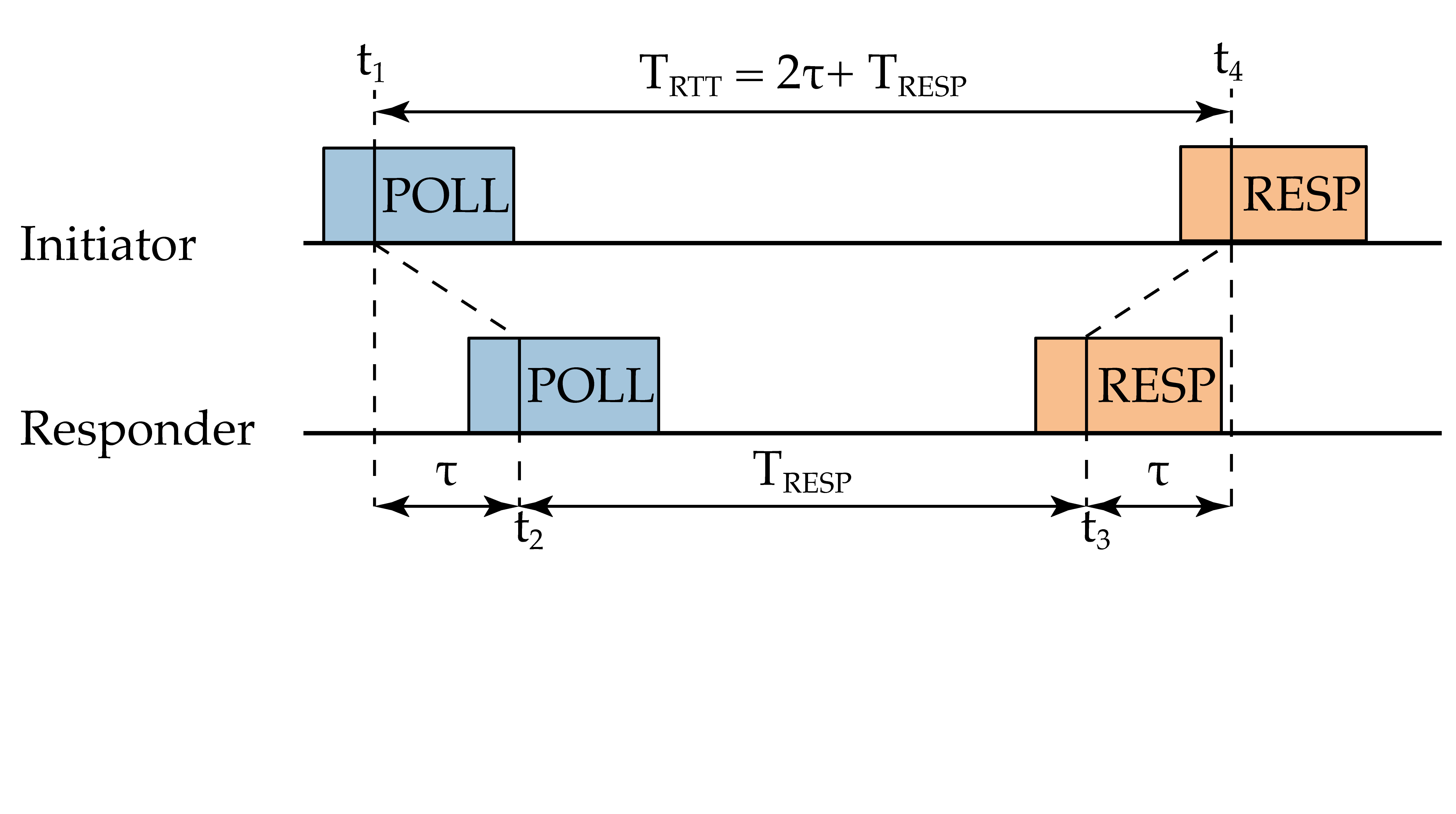
(a) Single-sided two-way ranging (SS-TWR).

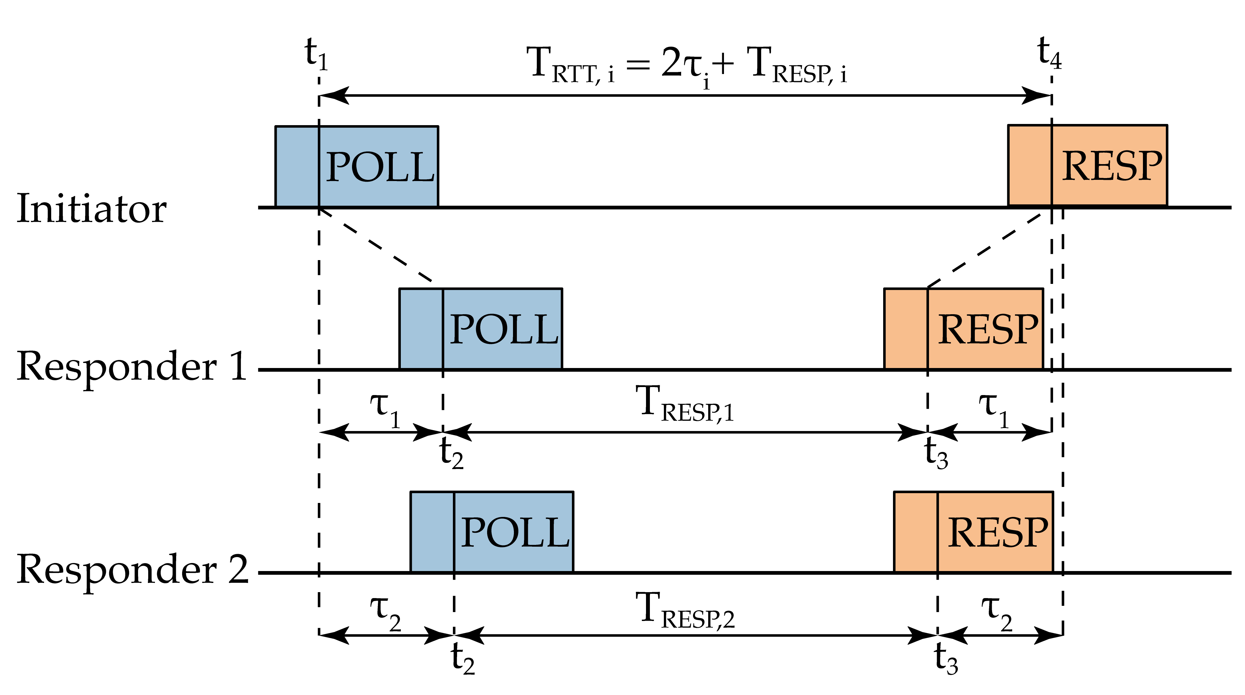
(b) Concurrent ranging.

Figure 1. In SS-TWR, the initiator transmits a unicast poll to which a single responder replies with a response. In concurrent ranging, the initiator transmits a broadcast poll to which responders in range reply concurrently.

UWB Two-way Ranging (TWR). Figure 1a illustrates single-sided two-way ranging (SS-TWR), the simplest scheme, part of the IEEE 802.15.4-2011 standard (std, 2011) and further illustrated in §2. The initiator requests a ranging measurement via a poll packet; the responder, after a known delay $T_{\mathit{RESP}}$, replies with a response packet containing the timestamps marking the receipt of poll and the sending of response. This information, along with the dual timestamps marking the sending of poll and the receipt of response measured locally at the initiator, enable the latter to accurately compute the time of flight $\tau$ and estimate the distance from the responder as $d=\tau\times c$, where $c$ is the speed of light in air.

Two-way ranging, as the name suggests, involves a pairwise exchange between the initiator and every responder. In other words, if the initiator must estimate its distance w.r.t. $N$ nodes, $2\times N$ packets are required. The situation is even worse with other schemes that improve accuracy by acquiring more timestamps via additional packet transmissions, e.g., up to $4\times N$ in popular double-sided two-way ranging (DS-TWR) schemes (Jiang and Leung, 2007; McLaughlin and Verso, 2018; Neirynck et al., 2016).

UWB Concurrent Ranging. We propose a novel approach to ranging in which, instead of separating the pairwise exchanges necessary to ranging, these are overlapping in time (Figure 1b). Its mechanics are extremely simple: when the single (broadcast) poll sent by the initiator is received, each responder sends back its response as if it were alone, effectively yielding concurrent replies to the initiator. This concurrent ranging technique enables the initiator to range with $N$ nodes at once by using only 2 packets, i.e., as if it were ranging against a single responder. This significantly reduces latency and energy consumption, increasing scalability and battery lifetime, but causes the concurrent signals from different responders to “fuse” in the communication channel, potentially yielding a collision at the initiator.

This is precisely where the peculiarities of UWB communications come into play. UWB transmissions rely on very short ($\leq$2 ns) pulses, enabling very precise timestamping of incoming radio signals. This is what makes UWB intrinsically more amenable to accurate ranging than narrowband, whose reliance on carrier waves that are more “spread in time” induces physical bounds on the precision that can be attained in establishing a time reference for an incoming signal. Moreover, it is what enables our novel idea of concurrent ranging. In narrowband, the fact that concurrent signals are spread over time makes them very difficult to tell apart once fused into a single signal. In practice, this is possible only if detailed channel state information is available—usually not the case on narrowband low-power radios, e.g., the popular CC2420 (Texas Instruments, [n.d.]) and its recent descendants. In contrast, the reliance of UWB on short pulses makes concurrent signals less likely to collide and combine therefore enabling, under certain conditions discussed later, their identification if channel impulse response (CIR) information is available. Interestingly, the DW1000 i) bases its own operation precisely on the processing of the CIR, and ii) makes the CIR available also to the application layer (§2).

Goals and Contributions. As discussed in §3, a strawman implementation of concurrent ranging is very simple. Therefore, using our prototype deployed in a small-scale setup, we begin by investigating the feasibility of concurrent ranging (§4), given the inevitable degradation in accuracy w.r.t. isolated ranging caused by the interference among the signals of responders, in turn determined by their relative placement. Our results, originally published in (Corbalán and Picco, 2018), offer empirical evidence that it is indeed possible to derive accurate ranging information from UWB signals overlapping in time.

On the other hand, these results also point out the significant challenges that must be overcome to transform concurrent ranging from an enticing opportunity to a practical system. Solving these challenges is the specific goal of this paper w.r.t. the original one (Corbalán and Picco, 2018) where, for the first time in the literature, we have introduced the concept and shown the feasibility of concurrent ranging.

Among these challenges, a key one is the limited precision of scheduling transmissions in commercial UWB transceivers. For instance, the popular Decawave DW1000 we use in this work can timestamp packet receptions (RX) with a precision of $\approx$15 ps, but can schedule transmissions (TX) with a precision of only $\approx$8 ns. This is not an issue in conventional ranging schemes like SS-TWR; as mentioned above, the responder embeds the necessary timestamps in the response payload, allowing the initiator to correct for the limited TX granularity. However, in concurrent ranging only one response is decoded, if any; the timing information of the others must be derived solely from the appearance of their corresponding signal paths in the CIR. This process is greatly affected by the TX uncertainty, which significantly reduces accuracy and consequently hampers the practical adoption of concurrent ranging.

In this paper, we tackle and solve this key challenge with a mechanism that significantly improves the TX scheduling precision via a local compensation (§5). Indeed, both the precise and imprecise information about TX scheduling are available at the responder; the problem arises because the radio discards the less significant 9 bits of the precise 40-bit timestamp. Therefore, the responder can correct for the known TX timing error when preparing its response. We achieve this by fine-tuning the frequency of the crystal oscillator entirely in firmware and locally to the responder, i.e., without additional hardware or external out-of-band infrastructure. Purposely, the technique also compensates for the oscillator frequency offset between initiator and responders, significantly reducing the impact of clock drift, the main cause of ranging error in SS-TWR.

Nevertheless, precisely scheduling transmissions is not the only challenge of concurrent ranging. A full-fledged, practically usable system also requires tackling i) the reliable identification of the concurrent responders, and ii) the precise estimation of the time of arrival (ToA) of their signals; both are complicated by the intrinsic mutual interference of concurrent transmissions. In this paper, we build upon techniques developed by us (Corbalán et al., 2019) and other groups (Großwindhager et al., 2018, 2019) since we first proposed concurrent ranging in (Corbalán and Picco, 2018). Nevertheless, we adapt and improve these techniques (§5) to accommodate the specifics of concurrent ranging in general and the TX scheduling compensation technique in particular. Interestingly, our novel design significantly increases not only the accuracy but also the reliability of concurrent ranging w.r.t. our original strawman design in (Corbalán and Picco, 2018). The latter relied heavily i) on the successful RX of at least one response, containing the necessary timestamps for accurate time-of-flight calculation, and ii) on the ToA estimation of this response performed by the DW1000, used to determine the difference in the signal ToA (and therefore distance) to the other responders. However, the fusion of concurrent signals may cause the decoding of the response to be matched to the wrong responder or fail altogether, yielding grossly incorrect estimates or none at all, respectively. Thanks to the ability to precisely schedule the TX of response packets, we i) remove the need to decode at least one of them, and ii) enable distance estimation solely based on the CIR. We can actually remove the payload entirely from response packets, further reducing latency and energy consumption.

We evaluate concurrent ranging extensively (§6). We first show via dedicated experiments that our prototype can schedule TX with $<1$ ns error. We then analyze the raw positioning information obtained by concurrent ranging, to assess its quality without the help of additional filtering techniques (Julier and Uhlmann, 1997; Wan and Van Der Merwe, 2000) that, as shown in (Tiemann et al., 2016; Guo et al., 2016; Hartmann et al., 2015; Ledergerber et al., 2015), would nonetheless improve performance. Our experiments in two environments, both with static positions and mobile trajectories, confirm that the near-perfect TX scheduling precision we achieve, along with our dedicated techniques to accurately extract distance information from the CIR, enable reliable decimeter-level ranging and positioning accuracy—same as conventional schemes for UWB but at a fraction of the network and energy cost.

These results, embodied in our prototype implementation, confirm that UWB concurrent ranging is a concrete option, immediately applicable to real-world applications where it strikes new trade-offs w.r.t. accuracy, latency, energy, and scalability, offering a valid (and often more competitive) alternative to established conventional methods, as discussed in §7.

Finally, in §8 we place concurrent ranging in the context of related work, before ending in §9 with brief concluding remarks.

2. Background

We concisely summarize the salient features of UWB radios in general (§2.1) and how they are made available by the popular DW1000 transceiver we use in this work (§2.2). Moreover, we illustrate the SS-TWR technique we build upon, and show how it is used to perform localization (§2.3).

2.1. Ultra-wideband in the IEEE 802.15.4 PHY Layer

UWB communications have been originally used for military applications due to their very large bandwidth and interference resilience to mainstream narrowband radios. In 2002, the FCC approved the unlicensed use of UWB under strict power spectral masks, boosting a new wave of research from industry and academia. Nonetheless, this research mainly focused on high data rate communications, and remained largely based on theory and simulation, as most UWB radios available then were bulky, energy-hungry, and expensive, hindering the widespread adoption of UWB. In 2007, the IEEE 802.15.4a standard amendment included a UWB PHY layer based on impulse radio (IR-UWB) (Win and Scholtz, 1998), aimed at providing accurate ranging with low-power consumption. A few years ago, Decawave released a standard-compliant IR-UWB radio, the DW1000, saving UWB from a decade-long oblivion, and taking by storm the field of real-time location systems (RTLS).

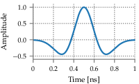
Figure 2. UWB pulse.

Figure 3. Distance resolution vs. bandwidth.

Impulse Radio. According to the FCC, UWB signals are characterized by a bandwidth $\geq 500$ MHz or a fractional bandwidth $\geq 20\%$ during transmission. To achieve such a large bandwidth, modern UWB systems are based on IR-UWB, using pulses (Figure 3) very narrow in time ($\leq 2$ ns). This reduces the power spectral density, the interference produced to other wireless technologies, and the impact of multipath components (MPC). Further, it enhances the ability of UWB signals to propagate through obstacles and walls (Yang and Giannakis, 2004) and simplifies transceiver design. The large bandwidth also provides excellent time resolution (Figure 3), enabling UWB receivers to precisely estimate the time of arrival (ToA) of a signal and distinguish the direct path from MPC. Time-hopping codes (Win and Scholtz, 2000) enable multiple access to the medium. Overall, these features make IR-UWB ideal for low-power ranging and localization as well as communication.

IEEE 802.15.4 UWB PHY Layer. The IEEE 802.15.4-2011 standard (std, 2011) specifies a PHY layer based on IR-UWB. The highest frequency at which a compliant device shall emit pulses is 499.2 MHz (fundamental frequency), yielding a standard chip duration of $\approx 2$ ns. A UWB frame is composed of i) a synchronization header (SHR) and ii) a data portion. The SHR is encoded in single pulses and includes a preamble for synchronization and the start frame delimiter (SFD), which delimits the end of the SHR and the beginning of the data portion. Instead, the data portion exploits a combination of burst position modulation (BPM) and binary phase-shift keying (BPSK), and includes a physical header (PHR) and the data payload. The duration of the preamble is configurable and depends on the number of repetitions of a predefined symbol, whose structure is determined by the preamble code. Preamble codes also define the pseudo-random sequence used for time-hopping in the transmission of the data part. The standard defines preamble codes of $31$ and $127$ elements, which are then interleaved with zeros according to a spreading factor. This yields a (mean) pulse repetition frequency ($\mathit{PRF}$) of $16$ MHz or $64$ MHz. Preamble codes and $\mathit{PRFs}$ can be exploited to configure non-interfering links within the same RF channel (Vecchia et al., 2019a).

2.2. Decawave DW1000

The Decawave DW1000 (Ltd., 2016a) is a commercially available low-power low-cost UWB transceiver compliant with IEEE 802.15.4, for which it supports frequency channels 1–4 in the low band and 5, 7 in the high band, and data rates of $110$ kbps, $850$ kbps, and $6.8$ Mbps. Channels 4 and 7 have a larger $900$ MHz bandwidth, while the others are limited to $499.2$ MHz.

Channel Impulse Response (CIR). The perfect periodic autocorrelation of the preamble code sequence enables coherent receivers to determine the CIR (Ltd., 2017), which provides information about the multipath propagation characteristics of the wireless channel between a transmitter and a receiver. The CIR allows UWB radios to distinguish the signal leading edge, commonly called direct or first path, from MPC and accurately estimate the ToA of the signal. In this paper, we exploit the information available in the CIR to perform these operations on several signals transmitted concurrently.

The DW1000 measures the CIR upon preamble reception with a sampling period $T_{s}=1.0016$ ns. The CIR is stored in a large internal buffer of 4096B accessible by the firmware developer. The time span of the CIR is the duration of a preamble symbol: 992 samples for a 16 MHz $\mathit{PRF}$ or 1016 for a 64 MHz $\mathit{PRF}$. Each sample is a complex number $a_{k}+jb_{k}$ whose real and imaginary parts are 16-bit signed integers. The amplitude $A_{k}$ and phase $\theta_{k}$ at each time delay $t_{k}$ is $A_{k}=\sqrt{\smash[b]{a_{k}^{2}+b_{k}^{2}}}$ and $\theta_{k}=\arctan{\frac{b_{k}}{a_{k}}}$. The DW1000 measures the CIR even when RX errors occur, therefore offering signal timing information even when a packet (e.g., a response) cannot be successfully decoded.

TX/RX Timestamps. The TX and RX timestamps enabling ranging are measured in a packet at the ranging marker (RMARKER) (Ltd., 2017), which marks the first pulse of the PHR after the SFD (§2.1). These timestamps are measured with a very high time resolution in radio units of $\approx$15.65\text{\,}\mathrm{ps}$$. The DW1000 first makes a coarse RX timestamp estimation, then adjusts it based on i) the RX antenna delay, and ii) the first path in the CIR estimated by a proprietary internal leading edge detection (LDE) algorithm. The CIR index that LDE determines to be the first path (FP_INDEX) is stored together with the RX timestamp in the RX_TIME register. LDE detects the first path as the first sampled amplitude that goes above a dynamic threshold based on i) the noise standard deviation $\sigma_{n}$ and ii) the noise peak value. Similar to the CIR, the RX signal timestamp is measured despite RX errors, unless there is a rare PHR error (Ltd., 2017, p. 97).

Delayed Transmissions. The DW1000 offers the capability to schedule transmissions at a specified time in the future (Ltd., 2017, p. 20), corresponding to the RMARKER. To this end, the DW1000 internally computes the time at which to begin the preamble transmission, considering also the TX antenna delay (Ltd., 2018). This makes the TX timestamp predictable, which is key for ranging.

Table 1. Current consumption comparison of DW1000 vs. TI CC2650 BLE SoC (Instruments, 2016) and Intel 5300 WiFi card (Halperin et al., 2010). Note that the CC2650 includes a 32-bit ARM Cortex-M3 processor and the Intel 5300 can support multiple antennas; further, consumption depends on radio configuration.

	DW1000	TI CC2650 (Instruments, 2016)	Intel 5300 (Halperin et al., 2010)
State	802.15.4a	BLE 4.2 & 802.15.4	802.11 a/b/g/n
Deep Sleep	50 $\mathrm{nA}$	100–150 $\mathrm{nA}$	N/A
Sleep	1 $\mathrm{\SIUnitSymbolMicro A}$	1 $\mathrm{\SIUnitSymbolMicro A}$	30.3  mA
Idle	12–18 mA	550 $\mathrm{\SIUnitSymbolMicro A}$	248 mA
TX	35–85 mA	6.1–9.1 mA	387–636 mA
RX	57–126 mA	5.9–6.1 mA	248–484 mA

Power Consumption. An important aspect of the DW1000 is its low-power consumption w.r.t. previous UWB transceivers (e.g.,  (Domain, 2011)). Table 1 compares the current consumption of the DW1000 against other commonly-used technologies (BLE and WiFi) for localization. The DW1000 consumes significantly less than the Intel 5300 (Halperin et al., 2010), which provides channel state information (CSI). However, it consumes much more than low-power widespread technologies such as BLE or IEEE 802.15.4 narrowband (Instruments, 2016). Hence, to ensure a long battery lifetime of UWB devices it is essential to reduce the radio activity, while retaining the accuracy and update rate of ranging and localization required by applications.

2.3. Time-of-Arrival (ToA) Ranging and Localization

In ToA-based methods, distance is estimated by precisely measuring RX and TX timestamps of packets exchanged between nodes. In this section, we describe the popular SS-TWR ranging technique (§2.3.1) we extend and build upon in this paper, and show how distance estimates from known positions can be used to determine the position of a target (§2.3.2).

2.3.1. Single-sided Two-way Ranging (SS-TWR)

In SS-TWR, part of the IEEE 802.15.4 standard (std, 2011), the initiator transmits a unicast poll packet to the responder, storing the TX timestamp $t_{1}$ (Figure 1a). The responder replies back with a response packet after a given response delay $T_{\mathit{RESP}}$. Based on the corresponding RX timestamp $t_{4}$, the initiator can compute the round trip time $T_{\mathit{RTT}}=t_{4}-t_{1}=2\tau+T_{\mathit{RESP}}$. However, to cope with the limited TX scheduling precision of commercial UWB radios, the response payload includes the RX timestamp $t_{2}$ of the poll and the TX timestamp $t_{3}$ of the response, allowing the initiator to precisely measure the actual response delay $T_{\mathit{RESP}}=t_{3}-t_{2}$. The time of flight $\tau$ can be then computed as

$$\tau=\frac{T_{\mathit{RTT}}-T_{\mathit{RESP}}}{2}=\frac{(t_{4}-t_{1})-(t_{3}-t_{2})}{2}$$

and the distance between the two nodes estimated as $d=\tau\times c$, where $c$ is the speed of light in air.

SS-TWR is simple, yet provides accurate distance estimation for many applications. The main source of error is the clock drift between initiator and responder, each running an internal oscillator with an offset w.r.t. the expected nominal frequency (Ltd., 2014), causing the actual time of flight measured by the initiator to be

$$\hat{\tau}=\frac{T_{\mathit{RTT}}(1+e_{I})-T_{\mathit{RESP}}(1+e_{R})}{2}$$

where $e_{I}$ and $e_{R}$ are the crystal offsets of initiator and responder, respectively. After some derivations, and by observing that $T_{\mathit{RESP}}\gg 2\tau$, we can approximate the error to (Jiang and Leung, 2007; Ltd., 2014)

$$\hat{\tau}-\tau\approx\frac{1}{2}T_{\mathit{RESP}}(e_{I}-e_{R})$$

Therefore, to reduce the ranging error of SS-TWR one should i) compensate for the drift, and ii) minimize $T_{\mathit{RESP}}$, as the error grows linearly with it.

2.3.2. Position Estimation

The estimated distance $\hat{d_{i}}$ to each of the $N$ responders can be used to determine the unknown initiator position $\mathbf{p}$, provided the responder positions are known. In two-dimensional space, the Euclidean distance $d_{i}$ to responder $R_{i}$ is defined by

(1) $$d_{i}=\left\lVert\mathbf{p}-\mathbf{p_{i}}\right\rVert=\sqrt{(x-x_{i})^{2}+(y-y_{i})^{2}}$$

where $\mathbf{p_{i}}=[x_{i},y_{i}]$ is the position of $R_{i}$, $i\in[1,N]$. The geometric representation of Eq. (1) is a circle (a sphere in 3D) with radius $d_{i}$ and center in $\mathbf{p_{i}}$. In the absence of noise, the intersection of $N\geq 3$ circles yields the unique initiator position $\mathbf{p}$. In practice, however, each distance estimate $\hat{d_{i}}=d_{i}+n_{i}$ suffers from an additive zero-mean measurement noise $n_{i}$. An estimate $\mathbf{\hat{p}}$ of the unknown initiator position can be determined (in 2D) by minimizing the non-linear least-squares (NLLS) problem

$$\mathbf{\hat{p}}=\operatorname*{arg\,min}_{\mathbf{p}}\sum_{i=1}^{N}\left(\hat{d}_{i}-\sqrt{(x-x_{i})^{2}+(y-y_{i})^{2}}\right)^{2}$$

In this paper, we solve the NLLS problem with state-of-the-art methods, as our contribution is focused on ranging and not on the computation of the position. Specifically, we employ an iterative local search via a trust region reflective algorithm (Branch et al., 1999). This requires an initial position estimate $\mathbf{p_{0}}$ that we set as the solution of a linear least squares estimator that linearizes the system of equations by applying the difference between any two of them (So, 2011; Fenwick, 1999).

3. Concurrent Ranging

Ranging against $N$ responders (e.g., anchors) with SS-TWR requires $N$ independent pairwise exchanges—essentially, $N$ instances of Figure 1a, one after the other. In contrast, the notion of concurrent ranging we propose obtains the same information within a single exchange, as shown in Figure 1b with only two responders. The technique is conceptually very simple, and consists of changing the basic SS-TWR scheme (§2.3.1) by:

1. replacing the $N$ unicast poll packets necessary to solicit ranging from the $N$ responders with a single broadcast poll, and

2. having all responders reply to the poll after the same time interval $T_{\mathit{RESP}}$ from its (timestamped) receipt.

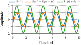
(a) Narrowband.

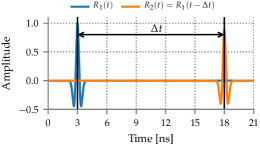
(b) UWB.

Figure 4. Concurrent ranging, idealized, with narrowband (4a) and UWB (4b) radios. With narrowband it is infeasible to recover the timing information of the signals from the individual responders. With UWB, instead, the different distance from the initiator to responders $R_{1}$ and $R_{2}$ produces a time shift $\Delta t$ between their signals. By measuring $\Delta t$, we can determine the distance difference ${\Delta d=\mid d_{1}-d_{2}\mid}$ between responders.

This simple idea is impractical (if not infeasible) in narrowband radios. As illustrated in the idealized view of Figure 4a, the signals from responders $R_{1}$ and $R_{2}$ interfere with each other, yielding a combined signal where the time information necessary to estimate distance is essentially lost. In contrast, Figure 4b shows why this is not the case in UWB; the time displacement $\Delta t$ of pulses from responders, caused by their different distances from the initiator, is still clearly visible in the resulting signal. This is due to the fact that UWB pulses are extremely short w.r.t. narrowband waves, and therefore unlikely to interfere—although in practice things are not so simple, as discussed in §4.

A Strawman Implementation. Concurrent ranging can be implemented very easily, a direct consequence of the simplicity of the concept. If a SS-TWR implementation is already available, it suffices to replace the unicast poll with a broadcast one. The computation of the actual ranging estimate requires processing the available CIR signal. The time shift $\Delta t$ can be measured as the difference between the first path from the closest responder $R_{1}$ in the CIR, automatically obtained from the DW1000 and used to compute the accurate distance estimate $d_{1}$, and the first path from $R_{2}$, that must be instead determined in a custom way, as discussed later (§4.4). Indeed, the first path from $R_{2}$, key to the operation of concurrent ranging, is treated as MPC or noise by the DW1000 but remains visible in the CIR, enabling computation of its time of arrival (ToA). Once $\Delta t$ is determined, the spatial displacement $\Delta d=c\Delta t$ can be computed, along with the distance $d_{2}=d_{1}+\Delta d$ of $R_{2}$; a similar process must be repeated in the case of $N$ responders.

As for the value of the response delay, crucial to the accuracy of SS-TWR (§2.3.1), our implementation uses $T_{\mathit{RESP}}=330$ $\mathrm{\SIUnitSymbolMicro s}$. We verified experimentally that this provides a good trade-off; lower values do not leave enough time to correctly prepare the radio for the response transmission, and larger ones negatively affect ranging due to clock drift.

In concurrent ranging, as in SS-TWR, the $T_{\mathit{RESP}}$ value also enables the responder to determine the time $t_{3}=t_{2}+T_{\mathit{RESP}}$ at which the response must be sent (Figure 1). The timestamp $t_{2}$ associated to the RX of poll is estimated by the DW1000 at the RMARKER with the extremely high precision of 15 ps (§2.1). Unfortunately, the same precision is not available when scheduling the delayed TX (§2.2) of the corresponding response at time $t_{3}$. Due to the significantly coarser granularity of TX scheduling in the DW1000, the TX of a response expected at a time $t_{3}$ actually occurs at $t+\epsilon$, with $\epsilon\in[-8,0)$ ns (Ltd., 2016a). This is not a problem in SS-TWR, as the timestamps $t_{2}$ and $t_{3}$ are embedded in the response and decoded by the initiator. Instead, in concurrent ranging the additional response packets are not decoded, and this technique cannot be used. Therefore, the uncertainty of TX scheduling, which at first may appear a negligible hardware detail, has significant repercussions on the practical exploitation of our technique, as discussed next.

4. Feasibility and Challenges: Empirical Observations

Although the idea of concurrent ranging is extremely simple and can be implemented straightforwardly on the DW1000, several questions must be answered to ascertain its practical feasibility. We discuss them next, providing answers based on empirical observations.

4.1. Experimental Setup

All our experiments employ the Decawave EVB1000 development platform (Ltd., 2013), equipped with the DW1000 transceiver, an STM32F105 ARM Cortex-M3 MCU, and a PCB antenna.

UWB Radio Configuration. We use a preamble length of 128 symbols and a data rate of 6.8 Mbps. Further, we use channel 4, whose wider bandwidth provides better resolution in determining the timing of the direct path and therefore better ranging estimates.

Firmware. We program the behavior of initiator and responder nodes directly atop Decawave libraries, without any OS layer, by adapting towards our goals the demo code provided by Decawave. Specifically, we provide support to log, via the USB interface, i) the packets transmitted and received, ii) the ranging measurements, and iii) the CIR measured upon packet reception.

Environment. All our experiments are carried out in a university building, in a long corridor whose width is 2.37 m. This is arguably a challenging environment due to the presence of strong multipath, but also very realistic to test the feasibility of concurrent ranging, given that one of the main applications of UWB is for localization in indoor environments.

Network Configuration. In all experiments, one initiator node and one or more responders are arranged in a line, placed exactly in the middle of the aforementioned corridor. This one-dimensional configuration allows us to clearly and intuitively relate the temporal displacements of the received signals to the spatial displacement of their source nodes. For instance, Figure 5 shows the network used in §4.2; we change the arrangement and number of nodes depending on the question under investigation.

4.2. Is Communication Even Possible?

Up to this point, we have implicitly assumed that the UWB transceiver is able to successfully decode one of the concurrent TX with high probability, similarly to what happens in narrowband and exploited, e.g., by Glossy (Ferrari et al., 2011) and other protocols (Ferrari et al., 2012; Landsiedel et al., 2013; Istomin et al., 2016). However, this may not be the case, given the different radio PHY and the different degree of synchronization (ns vs. $\mu$s) involved.

Figure 5. Experimental setup to investigate the reliability and accuracy of concurrent ranging (§4.2–§4.3). $I$ is the initiator, $R_{1}$ and $R_{2}$ are the responders.

Our first goal is therefore to verify this hypothesis. We run a series of experiments with three nodes, one initiator $I$ and two concurrent responders $R_{1}$ and $R_{2}$, placed along a line (Figure 5). The initiator is placed between responders at a distance $d_{1}$ from $R_{1}$ and $d_{2}=D-d_{1}$ from $R_{2}$, where $D=12$ m is the fixed distance between the responders. We vary $d_{1}$ between 0.4 m and 11.6 m in steps of 0.4 m. By changing the distance between initiator and responders we affect the chances of successfully receiving a packet from either responder due to the variation in power loss and propagation delay. For each initiator position, we perform 3,000 ranging exchanges with concurrent ranging, measuring the packet reception ratio ($\mathit{PRR}$) of response packets along with the resulting ranging estimates. As a baseline, we also performed 1,000 ranging exchanges with each responder in isolation, yielding $\mathit{PRR}=100\%$ for all initiator positions.

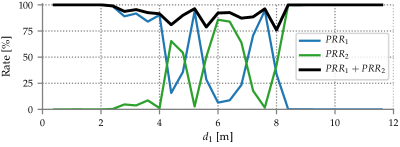
Figure 6. Packet reception rate ($\mathit{PRR}$) vs. initiator position $d_{1}$, with two concurrent transmissions.

Figure 6 shows the $\mathit{PRR}_{i}$ of each responder and the overall $\overline{\mathit{PRR}}=\mathit{PRR}_{1}+\mathit{PRR}_{2}$ denoting the case in which a packet from either responder is received correctly. Among all initiator positions, the worst overall $\overline{\mathit{PRR}}$ $=$ 75.93% is achieved for $d_{1}=8$ m. On the other hand, placing the initiator close to one of the responders (i.e., $d_{1}\leq 2$ m or $d_{1}\geq 10$ m) yields $\overline{\mathit{PRR}}\geq 99.9\%$. We also observe strong fluctuations in the center area. For instance, placing the initiator at $d_{1}=5.2$ m yields $\mathit{PRR}_{1}=93.6$% and $\mathit{PRR}_{2}=2.7$%, while nudging it at $d_{1}=6$ m yields $\mathit{PRR}_{1}=6.43$% and $\mathit{PRR}_{2}=85.73$%.

Summary. Overall, this experiment confirms the ability of the DW1000 to successfully decode, with high probability, one of the packets from concurrent transmissions.

4.3. How Concurrent Transmissions Affect Ranging Accuracy?

We also implicitly assumed that concurrent transmissions do not affect the ranging accuracy. In practice, however, the UWB wireless channel is far from being as “clean” as in the idealized view of Figure 4b. The first path is typically followed by several multipath reflections, which effectively create a “tail” after the leading signal. Depending on its temporal and spatial displacement, this tail may interfere with the first path of other responders by i) reducing its amplitude, or ii) generating MPC that can be mistaken for the first path, inducing estimation errors. Therefore, we now ascertain whether concurrent transmissions degrade ranging accuracy.

Baseline: Isolated Responders. We first look at the ranging accuracy for all initiator positions with each responder in isolation, using the same setup of Figure 5. Figure 7a shows the normalized histogram of the resulting ranging error from 58,000 ranging measurements. The average error is $\mu=1.7$ cm, with a standard deviation $\sigma=10.9$ cm. The maximum absolute error is 37 cm. The median of the absolute error is 8 cm, while the 99^th percentile is 28 cm. These results are in accordance with previously reported studies (Kempke et al., 2016a, 2015) employing the DW1000 transceiver.

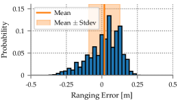
(a) Isolated responders.

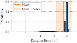
(b) Concurrent responders.

Figure 7. Normalized histogram of the ranging error with responders in isolation (Figure 7a) vs. two concurrent responders (Figure 7b). In the latter, the initiator sometimes receives the response from the farthest responder while estimating the first path from the closest one, therefore increasing the absolute error.

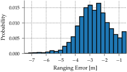
(a) Ranging Error $\in{[-7.5,-0.5]}$.

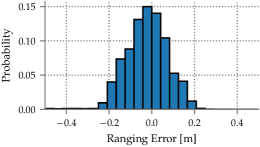
(b) Ranging Error $\in{[-0.5,0.5]}$.

Figure 8. Zoomed-in views of Figure 7b.

Concurrent Responders: Impact on Ranging Accuracy. Figure 7b shows the normalized histogram of the ranging error of 82,519 measurements using instead two concurrent responders. The median of the absolute error is 8 cm, as in the isolated case, while the 25^th and 75^th percentiles are 4 cm and 15 cm, respectively. However, while the average error $\mu=-0.42$ cm is comparable, the standard deviation $\sigma=1.05$ m is significantly higher. Further, the error distribution is clearly different w.r.t. the case of isolated responders (Figure 7a); to better appreciate the trends, Figure 8 offers a zoomed-in view of two key areas of the histogram in Figure 7b. Indeed, the latter has a long tail of measurements with significant errors; for 14.87% of the measured samples the ranging error is $<-0.5$ m, while in the isolated case the maximum absolute error only reaches 37 cm.

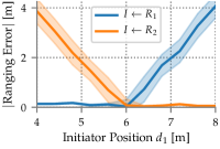
Figure 9. Ranging error vs. initiator position.

The Culprit: Mismatch between Received response and Nearest Responder. To understand why, we study the ranging error when the initiator is located in the center area ($4\leq d_{1}\leq 8$), the one with major $\mathit{PRR}$ fluctuations (Figure 6). Figure 9 shows the average absolute ranging error of the packets received from each responder as a function of the initiator position. Colored areas represent the standard deviation.

The ranging error of $R_{1}$ and $R_{2}$ increases dramatically for $d_{1}\geq 6$ m and $d_{2}\geq 6$ m, respectively. Moreover, the magnitude of the error exhibits an interesting phenomenon. For instance, when the initiator is at $d_{1}=6.8$ m, the average error for response packets received from $R_{1}$ is 1.68 m, very close to the displacement between responders, ${\Delta d=\mid d_{1}-d_{2}\mid=\mid 6.8-5.2\mid=1.6}$ m. Similarly, for $d_{1}=5.2$ m and $\Delta d=1.6$ m, the average error for the packets received from $R_{2}$ is 1.47 m.

The observation that the ranging error approximates the displacement $\Delta d$ between responders points to the fact that these high errors appear when the initiator receives the response from the farthest responder but estimates the first path of the signal with the CIR peak corresponding instead to the nearest responder. This phenomenon explains the high errors shown in Figure 7b and 8a, which are the result of this mismatch between the successful responder and the origin of the obtained first path. In fact, the higher probabilities in Figure 8a correspond to positions where the responder farther from the initiator achieves the highest $\mathit{PRR}_{i}$ in Figure 6. For example, for $d_{1}=7.6$ m, the far responder $R_{1}$ achieves $\mathit{PRR}_{1}=94.46$% and an average ranging error of $-3.27$ m, which again corresponds to $\Delta d=3.2$ m and also to the highest probability in Figure 8a.

The Role of TX Scheduling Uncertainty. When this mismatch occurs, we also observe a relatively large standard deviation in the ranging error. This is generated by the 8 ns TX scheduling granularity of the DW1000 transceiver (§3). In SS-TWR (Figure 1a), responders insert in the response the elapsed time $T_{\mathit{RESP}}=t_{3}-t_{2}$ between receiving the poll and sending the response. The initiator uses $T_{\mathit{RESP}}$ to precisely estimate the time of flight of the signal. However, the 8 ns uncertainty produces a discrepancy on $t_{3}$, and therefore between the $T_{\mathit{RESP}}$ used by the initiator and obtained from the successful response and the $T_{\mathit{RESP}}$ actually applied by the closest responder, resulting in significant error variations.

Summary. Concurrent transmissions can negatively affect ranging by producing a mismatch between the successful responder and the detected CIR path used to compute the time of flight. However, we also note that 84.59% of the concurrent ranging samples are quite accurate, achieving an absolute error $<30$ cm.

4.4. Does the CIR Contain Enough Information for Ranging?

In §3 we have mentioned that the limitation on the granularity of TX scheduling in the DW1000 introduces an 8 ns uncertainty. Given that an error of 1 ns in estimating the time of flight results in a corresponding error of $\approx$30 cm, this raises questions to whether the information in the CIR is sufficient to recover the timing information necessary for distance estimation.

Figure 10. Experimental setup to analyze the CIR resulting from concurrent ranging (§4.4).

We run another series of experiments using again three nodes but arranged slightly differently (Figure 10). We set $I$ and $R_{1}$ at a fixed distance $d_{1}=4$ m, and place $R_{2}$ at a distance $d_{2}>d_{1}$ from $I$; the two responders are therefore separated by a distance $\Delta d=d_{2}-d_{1}$. Unlike previous experiments, we increase $d_{2}$ in steps of 0.8 m; we explore $4.8\leq d_{2}\leq 12$ m, and therefore $0.8\leq\Delta d\leq 8$ m. For each position of $R_{2}$, we run the experiment until we successfully receive 500 response packets, i.e., valid ranging estimates; we measure the CIR on the initiator after each received response.

Baseline: Isolated Responders. Before using concurrent responders, we first measured the CIR of $R_{1}$ ($d_{1}=4$ m) in isolation. Figure 13 shows the average amplitude and standard deviation across 500 CIR signals, averaged by aligning them to the first path index (FP_INDEX) reported by the DW1000 (§2.2). The measured CIR presents an evident direct path at 50 ns, followed by strong multipath. We observe that the CIR barely changes across the 500 signals, exhibiting only minor variations in these MPCs (around 55–65 ns).

Concurrent Responders: Distance Estimation. We now analyze the effect of $R_{2}$ transmitting concurrently with $R_{1}$, and show how the distance of $R_{2}$ can be estimated. We focus on a single distance $d_{2}=9.6$ m and on a single CIR (Figure 13), to analyze in depth the phenomena at stake; we later discuss results acquired from 500 CIR signals (Figure 13) and for other $d_{2}$ values (Table 2).

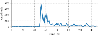
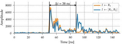
Figure 11. Average amplitude and standard deviation of 500 CIR signals for an isolated responder at $d_{1}=4$ m.

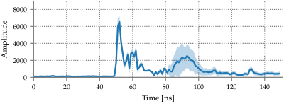
Figure 12. Impact of concurrent transmissions on the CIR. The response TX from $R_{2}$ introduces a second peak at a time shift $\Delta t=38$ ns after the direct path from $R_{1}$.

Figure 13. Average amplitude and standard deviation of 500 CIR signals, aligned based on the FP_INDEX, for two concurrent responders at distance ${d_{1}=4}$ m and ${d_{2}=9.6}$ m from the initiator.

Figure 13 shows that the response of $R_{2}$ introduces a second peak in the CIR, centered around 90 ns. This is compatible with our a-priori knowledge of $d_{2}=9.6$ m; the question is whether this distance can be estimated from the CIR.

Placing the direct path from $R_{2}$ in time constitutes a problem per se. In the case of $R_{1}$, this estimation is performed accurately and automatically by the DW1000, enabling an accurate estimate of $d_{1}$. The same could be performed for $R_{2}$ if it were in isolation, but not concurrently with $R_{1}$. Therefore, here we estimate the direct path from $R_{2}$ as the CIR index whose signal amplitude is closest to $20\%$ of the maximum amplitude of the peak—a simple technique used, e.g., in (Kempke et al., 2016b). The offset between the CIR index and the one returned by the DW1000 for $R_{1}$, for which a precise estimate is available, returns the delay $\Delta t$ between the responses of $R_{1}$ and $R_{2}$. We investigate more sophisticated and accurate techniques in §5.

The value of $\Delta t$ is induced by the propagation delay caused by the difference $\Delta d=d_{2}-d_{1}$ in the distance of the responders from the initiator. Recall the basics of SS-TWR (§2.3, Figure 1a) and of concurrent ranging (§3, Figure 1b). $R_{2}$ receives the poll from $I$ slightly after $R_{1}$; the propagation of the response back to $I$ incurs the same delay; therefore, the response from $R_{2}$ arrives at $I$ with a delay $\Delta t=2\times\frac{\Delta d}{c}$ w.r.t. $R_{1}$.

In our case, the estimate above from the CIR signal yields $\Delta t=38$ ns, corresponding to $\Delta d\approx 5.6$ m—indeed the displacement of the two responders. Therefore, by knowing the distance $d_{1}$ between $I$ and $R_{1}$, estimated precisely by the DW1000, we can easily estimate the distance between $I$ and $R_{2}$ as $d_{2}=d_{1}+\Delta d$. This confirms that a single concurrent ranging exchange contains enough information to reconstruct both distance estimates.

Concurrent Transmissions: Sources of Ranging Error. Another way to look at Figure 13 is to compare it against Figure 4b; while the latter provides an idealized view of what happens in the UWB channel, Figure 13 provides a real view. Multipath propagation and interference among the different paths of each signal affects the measured CIR; it is therefore interesting to see whether this holds in general and what is the impact on the (weaker) signal from $R_{2}$.

To this end, Figure 13 shows the average amplitude and standard deviation of 500 CIR signals aligned based on the FP_INDEX with $d_{1}=4$ m, and $d_{2}=9.6$ m. We observe that the first pulse, the one from the closer $R_{1}$, presents only minor variations in the amplitude of the direct path and of MPC, coherently with Figure 13. In contrast, the pulse from $R_{2}$ exhibits stronger variations, as shown by the colored area between 80 and 110 ns representing the standard deviation. However, these variations can be ascribed only marginally to interference with the pulse from $R_{1}$; we argue, and provide evidence next, that these variations are caused by the result of small time shifts of the observed CIR pulse, in turn caused by the $\epsilon\in[-8,0)$ ns TX scheduling uncertainty.

TX Uncertainty Affects Time Offsets. Figure 14 shows the normalized histogram, for the same 500 CIR signals, of the time offset $\Delta t$ between the times at which the responses from $R_{1}$ and $R_{2}$ are received at $I$. The real value, computed with exact knowledge of distances, is $\Delta t$ = 37.37 ns; the average from the CIR samples is instead $\Delta t$ $=36.11$ ns, with $\sigma=2.85$ ns. These values, and the trends in Figure 14, are compatible with the 8 ns uncertainty deriving from TX scheduling.

Time Offsets Affect Distance Offsets. As shown in Figure 14, the uncertainty in time offset directly translates into uncertainty in the distance offset, whose real value is $\Delta d=~{}5.6$ m. In contrast, the average estimate is $\Delta d=5.41$ m, with $\sigma=0.43$ m. The average error is therefore $-18$ cm; the 50^th, 75^th, and 99^th percentiles are 35 cm, 54 cm and 1.25 m, respectively. These results still provide sub-meter ranging accuracy as long as the estimated distance to $R_{1}$ is accurate enough.

Distance Offsets Affect Ranging Error. Recall that the distance $d_{1}$ from $R_{1}$ to $I$ is obtained directly from the timestamps provided by the DW1000, while for $R_{2}$ is estimated as $d_{2}=d_{1}+\Delta d$. Therefore, the uncertainty in the distance offset $\Delta d$ directly translates into an additional ranging error, shown in Figure 15 for each responder. $R_{1}$ exhibits a mean ranging error $\mu=3.6$ cm with $\sigma=1.8$ cm and a 99^th percentile over the absolute error of only 8 cm. Instead, the ranging error for $R_{2}$, computed indirectly via $\Delta d$, yields $\mu=-15$ cm with $\sigma=42.67$ cm. The median of the absolute error of $R_{2}$ is 31 cm, while the 25^th, 75^th, and 99^th percentiles are 16 cm, 58 cm, and 1.18 m, respectively.

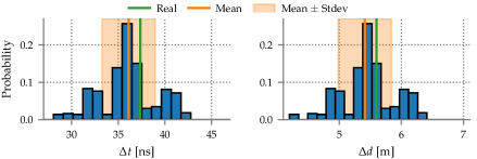
Figure 14. Normalized histograms of the time offset $\Delta t$ and corresponding distance offset $\Delta d$ between the leading CIR pulses from $R_{1}$ and $R_{2}$.

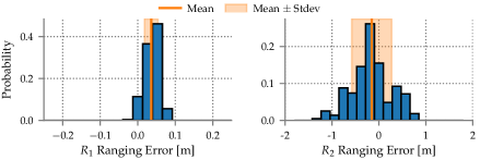
Figure 15. Normalized histograms of the concurrent ranging error of each responder.

Impact of Distance between Responders. In principle, the results above demonstrate the feasibility of concurrent ranging and its ability to achieve sub-meter accuracy. Nevertheless, these results were obtained for a single value of $d_{2}$. Table 2 summarizes the results obtained by varying this distance as described at the beginning of the section. We only consider the response packets successfully sent by $R_{1}$, since those received from $R_{2}$ produce the mismatch mentioned in §4.3, increasing the error by $\approx$ $\Delta d$; we describe a solution to this latter problem in §5.

Table 2. Concurrent ranging performance with two responders $R_{1}$ at a fixed distance $d_{1}=4$ m and $R_{2}$ at different distances $d_{2}=d_{1}+\Delta d$.

		$\mathit{PRR}$ [%]			$\mathbf{\Delta d}$ [m]		$\mathbf{R_{1}}$ Ranging Error [cm]					$\mathbf{R_{2}}$ Ranging Error [cm]
$\mathbf{d_{2}}$	$\mathbf{\Delta d}$	$PRR_{1}$	$PRR_{2}$	$\overline{\mathit{PRR}}$	$\mu$	$\sigma$	$\mu$	$\sigma$	50th	75th	99th	$\mu$	$\sigma$	50th	75th	99th
$\mathbf{4.8}$	$\mathbf{0.8}$	2.54	95.31	97.85	0.33	0.27	3	9	6	7	26	-43	32	30	73	105
$\mathbf{5.6}$	$\mathbf{1.6}$	36.3	36.73	73.03	1.5	0.38	6	2	6	8	12	-4	38	31	43	83
$\mathbf{6.4}$	$\mathbf{2.4}$	65.04	22.09	87.13	2.09	0.76	6	2	5	7	10	-25	76	51	113	161
$\mathbf{7.2}$	$\mathbf{3.2}$	0.2	99.6	99.8	3.0	0.0	8	0	8	8	8	-12	0	12	12	12
$\mathbf{8.0}$	$\mathbf{4.0}$	38.12	44.55	82.67	4.07	0.46	8	2	9	10	13	16	46	41	58	96
$\mathbf{8.8}$	$\mathbf{4.8}$	69.23	20.39	89.62	4.78	0.38	5	2	5	6	9	3	38	25	43	86
$\mathbf{9.6}$	$\mathbf{5.6}$	100.0	0.0	100.0	5.41	0.43	4	2	4	5	8	-15	43	31	58	118
$\mathbf{10.4}$	$\mathbf{6.4}$	94.76	2.52	97.28	6.42	0.44	5	2	5	7	9	7	44	36	53	99
$\mathbf{11.2}$	$\mathbf{7.2}$	85.05	5.23	90.27	7.16	0.4	6	2	6	7	10	2	39	34	42	97
$\mathbf{12.0}$	$\mathbf{8.0}$	100.0	0.0	100.0	8.06	0.35	4	2	5	6	9	11	35	29	44	77

To automatically detect the direct path of $R_{2}$, we exploit our a-priori knowledge of where it should be located based on $\Delta d$, and therefore $\Delta t$. We consider the slice of the CIR defined by $\Delta t\pm 8$ ns, and detect the first peak in it, estimating the direct path as the preceding index with the amplitude closest to the $20\%$ of the maximum amplitude, as described earlier. To abate false positives, we also enforce the additional constraints that a peak has a minimum amplitude of 1,500 and that the minimum distance between peaks is 8 ns.

As shown in Table 2, the distance to $R_{1}$ is estimated with an average error $\mu<9$ cm and $\sigma<10$ cm for all tested $d_{2}$ distances. The 99^th percentile absolute error is always $<27$ cm. These results are in line with those obtained in §4.3. As for $R_{2}$, we observe that the largest error of the estimated $\Delta d$, and of $d_{2}$, is obtained for the shortest distance $d_{2}=4.8$ m. In this particular setting, the pulses from both responders are very close and may even overlap in the CIR, increasing the resulting error, $\mu=-43$ cm for $d_{2}$. The other distances exhibit $\mu\leq 25$ cm. We observe that the error is significantly lower with $\Delta d\geq 4$ m, achieving $75^{\mathit{th}}<60$ cm for $d_{2}$. Similarly, for all $\Delta d\geq 4$ m except $\Delta d=5.6$ m, the 99^th percentile is $<1$ m. These results confirm that concurrent ranging can achieve sub-meter ranging accuracy, as long as the distance $\Delta d$ between responders is sufficiently large.

Summary. Concurrent ranging can achieve sub-meter accuracy, but requires i) a sufficiently large difference $\Delta d$ in distance (or $\Delta t$ in time) among concurrent responders, to distinguish the responders first paths within the CIR, and ii) a successful receipt of the response packet from the closest responder, otherwise the mismatch of responder identity increases the ranging error to $\approx\Delta d$.

4.5. What about More Responders?

We conclude the experimental campaign with our strawman implementation by investigating the impact of more than two concurrent responders, and their relative distance, on $\mathit{PRR}$ and ranging accuracy. If multiple responders are at a similar distance from the initiator, their pulses are likely to overlap in the CIR, hampering the discrimination of their direct paths from MPC. Dually, if the distance between the initiator and the nearest responder is much smaller w.r.t. the others, power loss may render the transmissions of farther responders too faint to be detected at the initiator, due to the interference from those of the nearest responder.

To investigate these aspects, we run experiments with five concurrent responders arranged in a line (Figure 16), for which we change the inter-node distance $d_{i}$. For every tested $d_{i}$, we repeat the experiment until we obtain 500 successfully received response packets, as done earlier.

Figure 16. Experimental setup to analyze the CIR resulting from five concurrent responders (§4.5).

Dense Configuration. We begin by examining a very short $d_{i}=0.4$ m, yielding similar distances between each responder and the initiator. In this setup, the overall ${\overline{\mathit{PRR}}=99.36}$%.

Nevertheless, recall that a time-of-flight difference of 1 ns translates into a difference of $\approx 30$ cm in distance and that the duration of a UWB pulse is $\leq 2$ ns; pulses from neighboring responders are therefore likely to overlap, as shown by the CIR in Figure 17a. Although we can visually observe different peaks, discriminating the ones associated to responders from those caused by MPC is very difficult, if not impossible, in absence of a-priori knowledge about the number of concurrent responders and/or the environment characteristics. Even when these are present, in some cases the CIR shows a wider pulse that “fuses” the pulses of one or more responders with MPC. In essence, when the difference in distance $\Delta d=d_{i}$ among responders is too small, concurrent ranging cannot be applied with the strawman technique we employed thus far; we address this problem in §5.

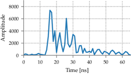
(a) $d_{i}=0.4$ m. The peaks corresponding to each responder are not clearly distinguishable; the distance from the initiator cannot be estimated.

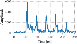
(b) $d_{i}=6$ m. The peaks corresponding to each responder are clearly separated; the distance from the initiator can be estimated.

Figure 17. Impact of the relative distance $d_{i}$ among 5 responders, analyzed via the corresponding CIR.

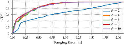
Figure 18. Impact of the relative distance $d_{i}$ among 5 responders: CDF of absolute ranging error.

Sparser Configurations: $\mathit{PRR}$. We now explore ${2\leq d_{i}\leq 10}$ m, up to a maximum distance $D~{}=~{}50$ m between the initiator $I$ and the last responder $R_{5}$. The experiment achieved an overall ${\overline{\mathit{PRR}}=96.59}$%, with the minimum $\overline{\mathit{PRR}}=88.2\%$ for the maximum $d_{i}=10$ m, and the maximum ${\overline{\mathit{PRR}}=100}$% for $d_{i}=8$ m. The closest responder $R_{1}$ achieved $\mathit{PRR}_{1}=90.56$%. The $\mathit{PRR}$ of the experiment is interestingly high, considering that in narrowband technologies increasing the number of concurrent transmitters sending different packets typically decreases reliability due to the nature of the capture effect (Landsiedel et al., 2013; Istomin et al., 2016). In general, the behavior of concurrent transmissions in UWB is slightly different—and richer—than in narrowband; the interested reader can find a more exhaustive treatment in (Vecchia et al., 2019a). In this specific case, the reason for the high $\mathit{PRR}$ we observed is the closer distance to the initiator of $R_{1}$ w.r.t. the other responders.

Sparser Configurations: Ranging Error. Figure 18 shows the CDF of the ranging error for all distances and responders. We use the same technique of §4.4 to detect the direct paths and, similarly, only consider the exchanges (about 90% in this case) where the successfully received response is from the nearest responder $R_{1}$, to avoid a mismatch (§4.3).

We observe the worst performance for $d_{i}=2$ m; peaks from different responders are still relatively close to each other and affected by the MPC of previously transmitted pulses. Instead, Figure 17b shows an example CIR for $d_{i}=6$ m, the intermediate value in the distance range considered. Five distinct peaks are clearly visible, enabling the initiator to estimate the distance to each responder. The time offset $\Delta t$ between two consecutive peaks is similar, as expected, given the same distance offset $\Delta d=d_{i}$ between two neighboring responders. This yields good sub-meter ranging accuracy for all $d_{i}\geq 4$, for which the average error is $\mu\leq 40$ cm and the absolute error $75^{\mathit{th}}\leq 60$ cm.

Summary. These results confirm that sub-meter concurrent ranging is feasible even with multiple responders. However, ranging accuracy is significantly affected by the relative distance between responders, which limits practical applicability.

5. Concurrent Ranging Reloaded

The experimental campaign in the previous section confirms that concurrent ranging is feasible, but also highlights several challenges not tackled by the strawman implementation outlined in §3, limiting the potential and applicability of our technique. In this section, we overcome these limitations with a novel design that, informed by the findings in §4, significantly improves the performance of concurrent ranging both in terms of accuracy and reliability, bringing it in line with conventional methods but at a fraction of the network and energy overhead.

We begin by removing the main source of inaccuracy, i.e., the 8 ns uncertainty in TX scheduling. The technique we present (§5.1) not only achieves sub-ns precision, as shown in our evaluation (§6.3), but also doubles as a mechanism to reduce the impact of clock drift, the main source of error in SS-TWR (§2.3.1). We then present our technique to correctly associate responders with paths in the CIR (§5.2), followed by two necessary CIR pre-processing techniques to discriminate the direct paths from MPC and noise (§5.3). Finally, we illustrate two algorithms for estimating the actual ToA of the direct paths and outline the overall processing that, by combining all these steps, yields the final distance estimation (§5.4).

5.1. Locally Compensating for TX Scheduling Uncertainty

The DW1000 transceiver can schedule a TX in the future with a precision of $4/(499.2\times 10^{6})\approx 8$ ns, much less than the signal timestamping resolution. SS-TWR responders circumvent this lack of precision by embedding the necessary TX/RX timestamps in their response. This is not possible in concurrent ranging, and an uncertainty $\epsilon$ from a uniform distribution $U[-8,0)$ ns directly affects concurrent transmissions from responders. The empirical observations in §4 show that mitigating this TX uncertainty is crucial to enhance accuracy. This section illustrates a technique, inspired by Decawave engineers during private communication, that achieves this goal effectively.

A key observation is that both the accurate desired TX timestamp and the inaccurate one actually used by the radio are known at the responder. Indeed, the DW1000 obtains the latter from the former by simply discarding its less significant 9 bits. Therefore, given that the responder knows beforehand the TX timing error that will occur, it can compensate for it while preparing its response.

We achieve this by fine-tuning the frequency of the oscillator, an operation that can be performed entirely in firmware and locally to the responder. In the technique described here, the compensation relies on the ability of the DW1000 to trim its crystal oscillator frequency (Ltd., 2017, p. 197) during operation. The parameter accessible via firmware is the radio trim index, whose value determines the correction currently applied to the crystal oscillator. By modifying the index by a given negative or positive amount (trim step) we can increase or decrease the oscillator frequency (i.e., clock speed) and compensate for the aforementioned known TX timing error. Interestingly, this technique can also be exploited to reduce the relative carrier frequency offset (CFO) between transmitter and receiver, with the effect of increasing receiver sensitivity, enhancing CIR estimation, and ultimately improving ranging accuracy and precision.

Trim Step Characterization. To design a compensation strategy, it is necessary to first characterize the impact of a trim step. To this end, we ran several experiments with a transmitter and a set of 6 receivers, to assess the impact on the CFO. The transmitter is initially configured with a trim index of 0, the minimum allowed, and sends a packet every 10 ms. After each TX, a trim step of +1 is applied, gradually increasing the index until 31, the maximum allowed, after which the minimum index of 0 is re-applied; increasing the trim index reduces the crystal frequency. Receivers do not apply a trim step; they use a fixed index of 15. For each received packet, we read the CFO between the transmitter and the corresponding receiver from the DW1000, which stores in the DRX_CONF register the receiver carrier integrator value (Ltd., 2016b, p. 80–81) measured during RX, and convert this value first to Hz and then to parts-per-million (ppm).

Figure 19 shows the CFO measured for each receiver as a function of the transmitter trim index, over $\geq$100,000 packets. If the CFO is positive (negative), the receiver local clock is slower (faster) than the transmitter clock (Ltd., 2016b, p. 81). All receivers exhibit a quasi-linear trend, albeit with a different offset. Across many experiments, we found that the average curve slope is $\approx-1.48$ ppm per unit trim step. This knowledge is crucial to properly trim the clock of the responders to match the frequency of the initiator and compensate for TX uncertainty, as described next.

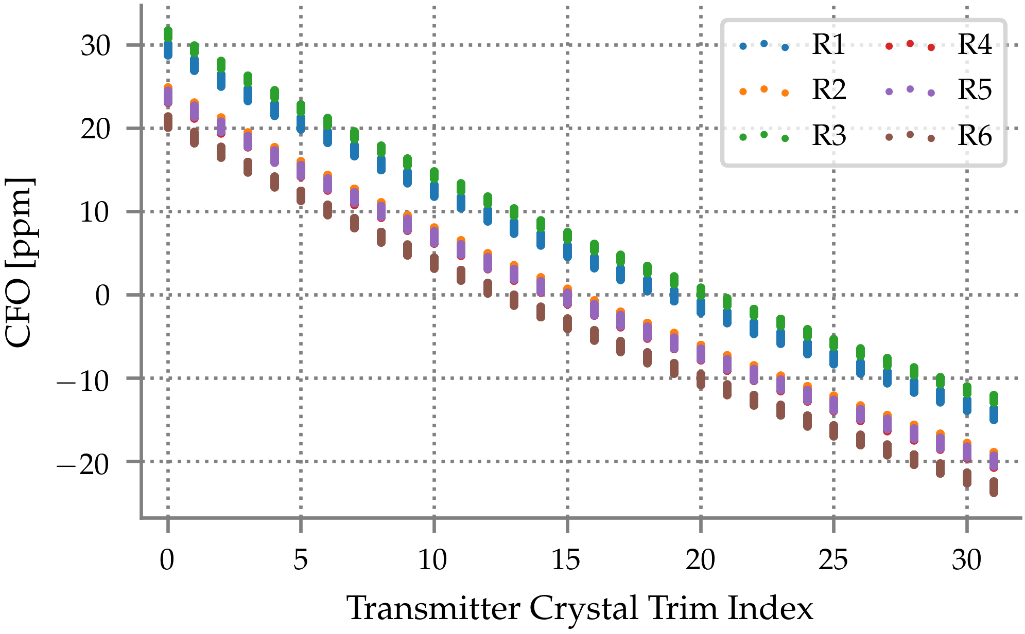
Figure 19. CFO between a transmitter and a set of six receivers, as a function of the transmitter trim index.

CFO Adjustment. After receiving the broadcast poll, responders obtain the CFO from their carrier integrator and trim their clock to better match the frequency of the initiator. For instance, if a given responder measures a CFO of $+3$ ppm, this means that its clock is slower than the initiator, and its frequency must be increased by applying a trim step of $-\frac{$3\text{\,}\mathrm{p}\mathrm{p}\mathrm{m}$}{$1.48\text{\,}\mathrm{p}\mathrm{p}\mathrm{m}$}\approx-2$. Repeating this adjustment limits at $\leq 1$ ppm the absolute value of the CFO between initiator and responders, reducing the impact of clock drift and improving RX sensitivity. Moreover, it also improves CIR estimation, enabling the initiator to better discern the signals from multiple, concurrent responders and estimate their ToA more accurately. Finally, this technique can be used to detune the clock (i.e., alter its speed), key to compensating for TX uncertainty.

TX Uncertainty Compensation. The DW1000 measures TX and RX times at the RMARKER (§2.2) with 40-bit timestamps in radio time units of $\approx 15.65$ ps. However, when scheduling transmissions, it ignores the lowest 9 bits of the desired TX timestamp. The known 9 bits ignored directly inform us of the TX error $\epsilon\in[-8,0)$ ns to be compensated for. The compensation occurs by temporarily altering the clock frequency via the trim index only for a given detuning interval, at the end of which the previous index is restored. Based on the known error $\epsilon$ and the predefined detuning interval $T_{\mathit{det}}$, we can easily compute the trim step $\mathcal{S}=\lfloor\frac{\epsilon}{$1.48\text{\,}\mathrm{p}\mathrm{p}\mathrm{m}$\times T_{\mathit{det}}}\rceil$ to be applied to compensate for the TX scheduling error. For instance, assume that a responder knows that its TX will be anticipated by an error $\epsilon=-5$ ns; its clock must be slowed down. Assuming a configured detuning interval $T_{\mathit{det}}=$400\text{\,}\mathrm{\SIUnitSymbolMicro s}$$, a trim step $\mathcal{S}=\lfloor\frac{$5\text{\,}\mathrm{n}\mathrm{s}$}{$1.48\text{\,}\mathrm{p}\mathrm{p}\mathrm{m}$\times$400\text{\,}\mathrm{\SIUnitSymbolMicro s}$}\rceil=\lfloor 8.45\rceil=8$ must be applied through the entire interval $T_{\mathit{det}}$. The rounding, necessary to map the result on the available integer values of the trim index, translates into a residual TX scheduling error. This can be easily removed, after the trim step $\mathcal{S}$ is determined, by recomputing the detuning interval as $T_{\mathit{det}}=\frac{\epsilon}{$1.48\text{\,}\mathrm{p}\mathrm{p}\mathrm{m}$\times\mathcal{S}}$, equal to $422.3\text{\,}\mathrm{\SIUnitSymbolMicro s}$ in our example. Indeed, the duration of $T_{\mathit{det}}$ can be easily controlled in firmware and with a significantly higher resolution than the trim index, yielding a more accurate compensation.

Implementation. In our prototype, we determine the trim step $\mathcal{S}$, adjust the CFO, and compensate the TX scheduling error in a single operation. While detuning the clock, we set the data payload and carry out the other operations necessary before TX, followed by an idle loop until the detuning interval is over. We then restore the trim index to the value determined during CFO adjustment and configure the DW1000 to transmit the response at the desired timestamp. To compensate for an error $\epsilon\in[-8,0)$ ns without a very large trim step (i.e., abrupt changes of the trim index) we set a default detuning interval $T_{\mathit{det}}=$560\text{\,}\mathrm{\SIUnitSymbolMicro s}$$ and increase the ranging response delay to $T_{\mathit{RESP}}=$800\text{\,}\mathrm{\SIUnitSymbolMicro s}$$. This value is higher than the one ($T_{\mathit{RESP}}=$330\text{\,}\mathrm{\SIUnitSymbolMicro s}$$) used in §4 and, in general, would yield worse SS-TWR ranging accuracy due to a larger clock drift (§2.3). Nevertheless, here we directly limit the impact of the clock drift with the CFO adjustment, precisely scheduling transmissions with $<1$ ns errors, as shown in §6.3; therefore, in practice, the minor increase in $T_{\mathit{RESP}}$ bears little to no impact.

5.2. Response Identification

As observed in §4, if the distance between the initiator and the responders is similar, their paths and MPC overlap in the CIR, hindering responder identification and ToA estimation. Previous work (Großwindhager et al., 2018) proposed to assign a different pulse shape to each responder and then use a matched filter to associate paths with responders. However, this leads to responder mis-identifications, as we showed in (Corbalán et al., 2019), because the channel cannot always be assumed to be separable, i.e., the measured peaks in the CIR can be a combination of multiple paths, and the received pulse shapes can be deformed, creating ambiguity in the matched filter output.

To reliably separate and identify responders, we resort to response position modulation (Großwindhager et al., 2018), whose effectiveness has instead been shown by our own work on Chorus (Corbalán et al., 2019) and by SnapLoc (Großwindhager et al., 2019). The technique consists of delaying each response by $\delta_{i}=(i-1)T_{\mathit{ID}}$, where $i\in\{1,N\}$ is the responder identifier. The resulting CIR consists of an ordered sequence of signals that are time-shifted based on i) the assigned delays $\delta_{i}$, and ii) the propagation delays $\tau_{i}$, as shown in Figure 21.

The constant $T_{\mathit{ID}}$ must be set according to i) the CIR time span, ii) the maximum propagation time, as determined by the dimensions of the target deployment area, and iii) the multipath profile in it. Figure 20 shows the typical power decay profile in three different environments obtained from the IEEE 802.15.4a radio model (Molisch et al., 2004). MPC with a time shift $\geq 60$ ns suffer from significant power decay w.r.t. the direct path. Therefore, by setting $T_{\mathit{ID}}=128$ ns as in (Corbalán et al., 2019; Großwindhager et al., 2019) we are unlikely to suffer from significant MPC and able to reliably distinguish the responses. Moreover, considering that the DW1000 CIR has a maximum time span of $~{}\approx 1017$ ns, we can accommodate up to 7 responders, leaving a small portion of the CIR with only noise. We observe that this technique relies on the correct identification of the first and last responder to properly reconstruct the sequence, and avoid mis-identifications; our evaluation (§6) shows that these rarely occur in practice.

Figure 20. Power decay profile in different environments according to the IEEE 802.15.4a radio model (Molisch et al., 2004).

Finally, although the technique is similar to the one in (Corbalán et al., 2019; Großwindhager et al., 2019), the different context in which it is applied yields significant differences. In these systems, the time of flight $\tau_{i}$ is known and compensated for, based on the fixed and known position of anchors. In concurrent ranging, not only $\tau_{i}$ is not known a priori, but it also has a twofold impact on the response RX timestamps, making the problem more challenging. On the other hand, concurrent ranging is more flexible as it does not rely on the known position of anchors. Further, as packet exchanges are triggered by the initiator rather than the anchors as in (Corbalán et al., 2019; Großwindhager et al., 2019), the former could determine time shifts on a per-exchange basis, assigning a different $\delta_{i}$ to each responder via the broadcast poll. For instance, in a case where responders $R_{i}$ and $R_{i+1}$ have a distance $d_{i}\gg d_{i+1}$ from the initiator, a larger time shift $\delta_{i+1}$ could help separating the pulse of $R_{i+1}$ from the MPC of $R_{i}$. Similarly, when more responders are present than what can be accommodated in the CIR, the initiator could dynamically determine the responders that should reply and the delays $\delta_{i}$ they should apply. This adaptive, initiator-based time shift assignment opens several intriguing opportunities, especially for mobile, ranging-only applications; we are currently investigating them as part of our ongoing work (§7).

5.3. CIR Pre-processing

We detail two techniques to reorder the CIR array and estimate the signal noise standard deviation $\sigma_{n}$. These extend and significantly enhance the techniques we originally proposed in (Corbalán et al., 2019), improving the robustness and accuracy of the ToA estimation algorithms in §5.4.1.

5.3.1. CIR Array Re-arrangement

In the conventional case of an isolated transmitter, the DW1000 arranges the CIR signal by placing the first path at FP_INDEX $\approx 750$ in the accumulator buffer (§2.2). In concurrent ranging, one would expect the FP_INDEX to similarly indicate the direct path of the first responder $R_{1}$, i.e., the one with the shorter time shift $\delta_{1}=0$. Unfortunately, this is not necessarily the case, as the FP_INDEX can be associated with the direct path of any of the involved responders (Figure 21). Further, and worse, due to the TX time shifts $\delta_{i}$ we apply in concurrent ranging, the paths associated to the later responders may be circularly shifted at the beginning of the array, disrupting the implicit temporal ordering at the core of responder identification (§5.2).

Therefore, before estimating the ToA of the concurrent signals, we must i) re-arrange the CIR array to match the order expected from the assigned time shifts, and ii) correspondingly re-assign the index associated to the FP_INDEX and whose timestamp is available in radio time units. In (Corbalán et al., 2019) we addressed a similar problem by partially relying on knowledge of the responder ID contained in the response payload (among the several concurrent ones) actually decoded by the radio, which then usually places its corresponding first path at FP_INDEX $\approx 750$ in the CIR. However, this technique relies on successfully decoding a response, which is unreliable as we previously observed in §4. Here, we remove this dependency and enable a correct CIR re-arrangement even in cases where the initiator is unable to successfully decode any response, significantly improving reliability.

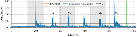
(a) Raw CIR array.

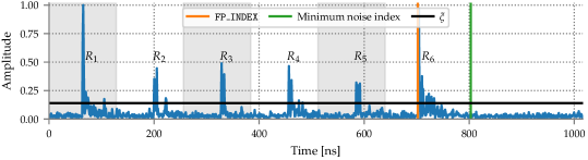
(b) Re-arranged CIR array.

Figure 21. CIR re-arrangement. The DW1000 measured the FP_INDEX as the direct path of $R_{6}$ in the raw CIR (Figure 21a). After finding the CIR sub-array with the lowest noise, we re-arrange the CIR (Figure 21b) setting the response of $R_{1}$ at the beginning and the noise-only sub-array at the end.

We achieve this goal by identifying the portion of the CIR that contains only noise, which appears in between the peaks of the last and first responders. First, we normalize the CIR w.r.t. its maximum amplitude sample and search for the CIR sub-array of length $W$ with the lowest sum—the aforementioned noise-only portion. Next, we determine the index at which this noise sub-array begins (minimum noise index in Figure 21) and search for the next sample index whose amplitude is above a threshold $\xi$. This latter index is a rough estimate of the direct path of $R_{1}$, the first expected responder. We then re-order the CIR array by applying a circular shift, setting the $N$ responses at the beginning of the array, followed by the noise-only portion at the end. Finally, we re-assign the index corresponding to the original FP_INDEX measured by the DW1000 and whose radio timestamp is available.

We empirically found, by analyzing 10,000s of CIRs signals, that a threshold $\xi\in[0.12,0.2]$ yields an accurate CIR reordering. Lower values may cause errors due to noise or MPC, while higher values may disregard a weak first path from $R_{1}$. The noise window $W$ must be set based on the CIR time span, the time shifts $\delta_{i}$ applied, and the number $N$ of concurrent responders. Hereafter, we set $\xi=0.14$ and $W=228$ samples with $N=6$ responders and $T_{\mathit{ID}}=128$ ns.

5.3.2. Estimating the Noise Standard Deviation

ToA estimation algorithms frequently rely on a threshold derived from the noise standard deviation $\sigma_{n}$, to detect the first path from noise and MPC. The DW1000 estimates $\sigma_{n}^{DW}$ based on the measured CIR (Ltd., 2017). However, in the presence of concurrent transmissions, the DW1000 sometimes yields a significantly overestimated $\sigma_{n}^{DW}$, likely because it considers the additional response signals as noise. Therefore, we recompute our own estimate of $\sigma_{n}$ as the standard deviation of the last 128 samples of the re-arranged CIR (Figure 21b). By design (§5.3.1) these samples belong to the noise-only portion at the end of the re-arranged CIR, free from MPC from responses; the noise estimate is therefore significantly more reliable than the one computed by the DW1000, meant for non-concurrent ranging.

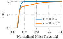
Figure 22. Threshold comparison.

Figure 22 offers evidence of this last statement by comparing the two techniques across the 9,000 signals with $N=6$ concurrent responders we use in §6.4 to evaluate the performance of concurrent ranging with the initiator placed in 18 different static positions. The chart shows the actual noise threshold computed as $\eta=11\times\sigma_{n}$, which we empirically found to be a good compromise for ToA estimation (§5.4.1). Using our technique, $\eta$ converges to a $99^{\mathit{th}}$ percentile of $0.213$ over the normalized CIR amplitude, while the default $\sigma_{n}^{DW}$ yields $99^{\mathit{th}}=0.921$; this value would lead to discard most of the peaks from concurrent responders. For instance, in Figure 21 only 2 out of 6 direct paths would be detected with such a high threshold. Across these 9,000 signals, using our estimated $\sigma_{n}$ instead of $\sigma_{n}^{DW}$ increases the ranging and localization reliability of concurrent ranging by up to $16\%$ depending on the ToA algorithm used, as we explain next.

5.4. From Time to Distance

Enabling concurrent ranging on the DW1000 requires a dedicated algorithm (§5.4.1) to estimate the ToA of each response in the CIR. This timing information must then be translated into the corresponding distances (§5.4.2), used directly or in the computation of the initiator position (§2.3.2).

5.4.1. Time of Arrival Estimation

To determine the first path of each responder, we use FFT to upsample the re-arranged CIR signals by a factor $L=30$, yielding a resolution $T_{s}\approx 33.38$ ps. We then split the CIR into chunks of length equal to the time shift $T_{\mathit{ID}}$ used for responder identification (§5.2), therefore effectively separating the signals of each response. Finally, the actual ToA estimation algorithm is applied to each chunk, yielding the CIR index $\mathcal{T}_{i}$ marking the ToA of each responder $R_{i}$. We consider two ToA estimation algorithms:

• Threshold-based. This commonly-used algorithm simply places the first path at the first $i^{\mathit{th}}$ index whose sampled amplitude $A_{i}>\eta$, where $\eta$ is the noise threshold (§5.3).

• Search and Subtract (S&S). This well-known algorithm has been proposed in (Falsi et al., 2006); here, we use our adaptation (Corbalán et al., 2019) to the case of concurrent transmissions. S&S determines the $K$ strongest paths, considering all signal paths whose peak amplitude $A_{i}>\eta$. The first path is then estimated as the one with the minimum time delay, i.e., minimum index in the CIR chunk.

These two algorithms strike different trade-offs w.r.t. complexity, accuracy, and resilience to multipath. The threshold-based algorithm is very simple and efficient but also sensitive to high noise. For instance, if a late MPC from a previous chunk appears at the beginning of the next one with above-threshold amplitude, it is selected as the first path, yielding an incorrect ToA estimate. S&S is more resilient, as these late MPC from previous responses would need to be stronger than the $K$ strongest paths from the current chunk to cause a mismatch. Still, when several strong MPC are in the same chunk, S&S may incorrectly select one of them as the first path, especially if the latter is weaker than MPC. Moreover, S&S relies on a matched filter, which i) requires to determine the filter template by measuring the shape of the transmitted UWB pulses, and ii) increases computational complexity, as $K$ discrete convolutions must be performed to find the $K$ strongest paths.

We compare these ToA estimation algorithms in our evaluation (§6).

5.4.2. Distance Estimation

These ToA estimation algorithms determine the CIR indexes $\mathcal{T}_{i}$ marking the direct path of each response. These, however, are only array indexes; each must be translated into a radio timestamp marking the time of arrival of the corresponding response, and combined with other timing information to reconstruct the distance $d_{i}$ between initiator and responder.

In §3–§4 we relied on the fact that the radio directly estimates the ToA of the first responder $R_{1}$ with high accuracy, enabling accurate distance estimation by using the timestamps embedded in the payload. Then, by looking at the time difference $\Delta t_{i,1}$ between the first path of $R_{1}$ and another responder $R_{i}$ we can determine its distance from the initiator as $d_{i}=d_{1}+c\frac{\Delta t_{i,1}}{2}$. This approach assumes that the radio i) places the direct path of $R_{1}$ at the FP_INDEX and ii) successfully decodes the response from $R_{1}$, containing the necessary timestamps to accurately determine $d_{1}$. However, the former is not necessarily true (Figure 21); as for the latter, the radio may receive the response packet from any responder or none. Therefore, we cannot rely on the distance estimation of $R_{1}$.

Interestingly, the compensation technique to eliminate the TX scheduling uncertainty (§5.1) is also key to enable an alternate approach avoiding these issues and yielding additional benefits. Indeed, this technique enables TX scheduling with sub-ns accuracy (§6.3). Therefore, the response delay $T_{\mathit{RESP}}$ and the additional delay $\delta_{i}$ for responder identification in concurrent ranging can be enforced with high accuracy, without relying on the timestamps embedded in the response.

In more detail, the time of flight $\tau_{\mathit{i}}$ from the initiator to responder $R_{i}$ is estimated as

(2) $$\tau_{\mathit{i}}=\frac{T_{\mathit{RTT,i}}-T_{\mathit{RESP,i}}}{2}$$

and the corresponding distance as $d_{i}=c\times\tau_{\mathit{i}}$. As shown in Figure 23, $T_{\mathit{RESP,i}}$ is the delay between the RX of poll and the TX of response at responder $R_{i}$. This delay is computed as the addition of three factors $T_{\mathit{RESP,i}}=T_{\mathit{RESP}}+\delta_{i}+A_{\mathit{TX}}$, where $T_{\mathit{RESP}}$ is the fixed response delay inherited from SS-TWR (§2.3.1), $\delta_{i}=(i-1)T_{\mathit{ID}}$ is the responder-specific delay enabling response identification (§5.2), and $A_{\mathit{TX}}$ is the known antenna delay obtained in a previous calibration step (Ltd., 2018).

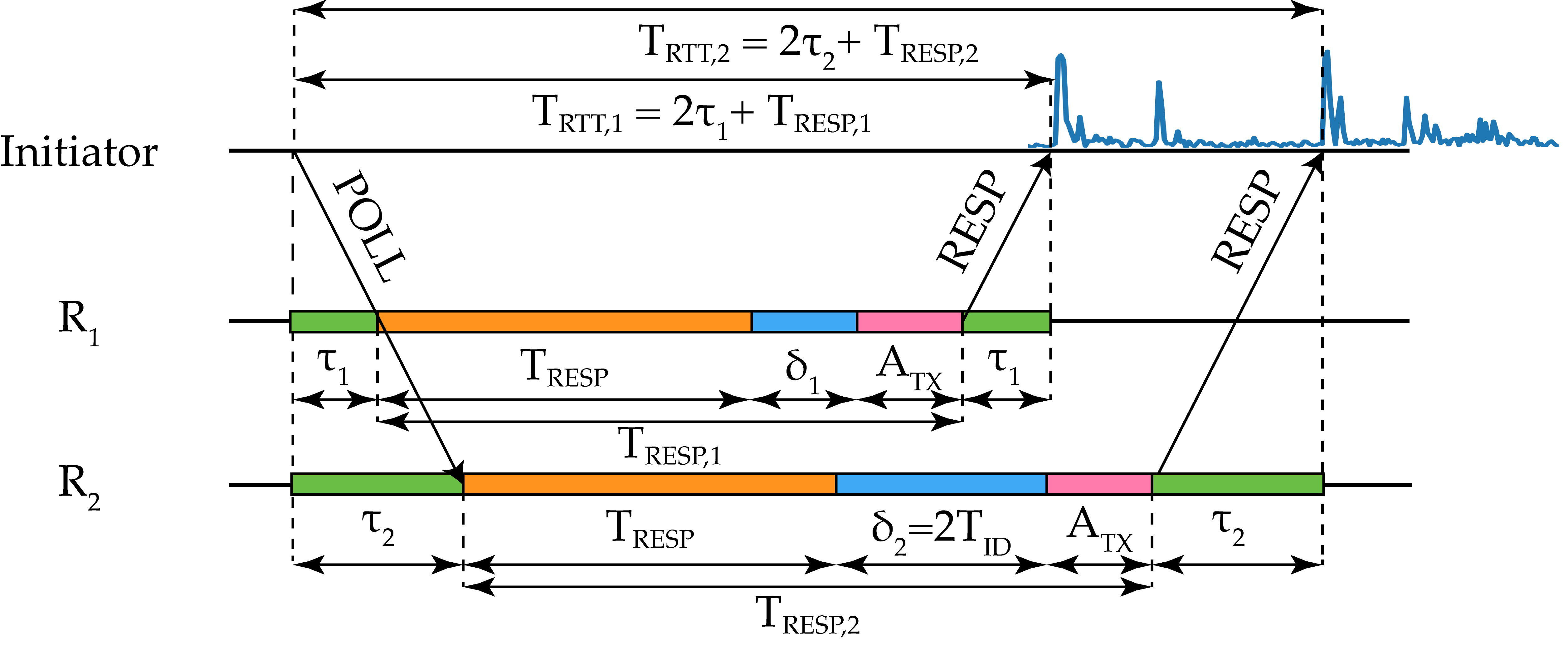
Figure 23. Concurrent ranging time of flight $\tau_{i}$ computation. To determine the distance $d_{i}=c\times\tau_{i}$ to responder $R_{i}$, we need to accurately measure the actual response delay $T_{\mathit{RESP,i}}=T_{\mathit{RESP}}+\delta_{i}+A_{\mathit{TX}}$ and the round-trip time $T_{\mathit{RTT,i}}$ of each responder based on our ToA estimation.

$T_{\mathit{RTT,i}}$ is the round-trip time for responder $R_{i}$, measured at the initiator as the difference between the response RX timestamp and the poll TX timestamp. The latter is accurately determined at the RMARKER by the DW1000, in device time units of $\approx 15.65$ ps, while the former must be extracted from the CIR via ToA estimation. Nevertheless, the algorithms in §5.4.1 return only the CIR index $\mathcal{T}_{i}$ at which the first path of responder $R_{i}$ is estimated; this index must therefore be translated into a radio timestamp, similar to the TX poll one. To this end, we rely on the fact that the precise timestamp $T_{\mathit{FP}}$ associated to the FP_INDEX in the CIR is known. Therefore, it serves as the accurate time baseline w.r.t. which to derive the response RX by i) computing the difference $\Delta\mathcal{T}_{\mathit{FP,i}}=\texttt{FP\_INDEX}-\mathcal{T}_{i}$ between the indexes in the CIR, and ii) obtaining the actual RX timestamp as $T_{\mathit{FP}}-T_{s}\times\Delta\mathcal{T}_{\mathit{FP,i}}$, where $T_{s}$ is the CIR sampling period after upsampling (§5.4.1).

In our experiments, we noticed that concurrent ranging usually underestimates distance. This is due to the fact that the responder estimates the ToA of poll with the DW1000 LDE algorithm, while the initiator estimates the ToA of each response with one of the algorithms in §5.4.1. For instance, S&S measures the ToA at the beginning of the path, while LDE measures it at a peak height related to the noise standard deviation reported by the DW1000. This underestimation is nonetheless easily compensated by a constant offset ($\leq 20$ cm) whose value can be determined during calibration at deployment time.

Together, the steps we described enable accurate estimation of the distance to multiple responders solely based on the CIR and the (single) RX timestamp provided by the radio. In the DW1000, i) the CIR is measured and available to the application even if RX errors occur, and ii) the RX timestamp necessary to translate our ToA estimates to radio timestamps is always updated, therefore making our concurrent ranging prototype highly resilient to RX errors. Finally, the fact that we remove the dependency on $R_{1}$ and therefore no longer need to embed/receive any timestamp enables us to safely remove the entire payload from response packets. Unless application information is piggybacked on a response, this can be composed only of preamble, SFD, and PHR, reducing the length of the response packet, and therefore the latency and energy consumption of concurrent ranging.

6. Evaluation

We evaluate our concurrent ranging prototype, embodying the techniques illustrated in §5. We begin by describing our experimental setup (§6.1) and evaluation metrics (§6.2). Then, we evaluate our TX scheduling (§6.3), confirming its ability to achieve sub-ns precision. This is key to improve the accuracy of ranging and localization, which we evaluate in static positions (§6.4) and via trajectories generated by a mobile robot in an OptiTrack facility (§6.5).

6.1. Experimental Setup

We implemented concurrent ranging atop Contiki OS (Corbalán et al., 2018) using the EVB1000 platform (Ltd., 2013) as in §4.

UWB Radio Configuration. In all experiments, we set the DW1000 to use channel 7 with center frequency $f_{c}=6489.6$ GHz and $900$ MHz receiver bandwidth. We use the shortest preamble length of 64 symbols with preamble code 17, the highest $PRF=64~{}$MHz, and the highest 6.8 Mbps data rate. Finally, we set the response delay $T_{\mathit{RESP}}=$ $800\text{\,}\mathrm{\SIUnitSymbolMicro s}$ to provide enough time to compensate for the TX scheduling uncertainty (§5.1).

Concurrent Ranging Configuration. Table 3 summarizes the default values of concurrent ranging parameters. The time shift $T_{\mathit{ID}}=128$ ns for response identification (§5.2) corresponds to a distance of $38.36$ m, sufficiently larger than the maximum distance difference ($\approx 12$ m) among anchors in our setups. For ToA estimation (§5.4.1), we use a noise threshold $\eta=11\times\sigma_{n}$, computed as described in §5.3, and $K=3$ iterations per CIR chunk of the S&S algorithm.

Table 3. Main parameters of concurrent ranging with default values.

Symbol	Description	Default Value
$L$	CIR upsampling factor	30
$T_{\mathit{ID}}$	Time shift for response identification	128 ns
$\xi$	Noise threshold for CIR re-arrangement	0.14
$W$	Window length for CIR re-arrangement	228 samples
$\eta$	Noise threshold for ToA estimation algorithm	$11\times\sigma_{n}$
$K$	Iterations (max. number of paths) of the S&S ToA algorithm	3

Infrastructure. We run our experiments with a mobile testbed infrastructure we deploy in the target environment. Each testbed node consists of an EVB1000 (Ltd., 2013) connected via USB to a Raspberry Pi (RPi) v3, equipped with an ST-Link programmer enabling firmware uploading. Each RPi reports its serial data via WiFi to a server, which stores it in a log file. Although our prototype supports runtime positioning, hereafter we run our analysis offline.

In each test, we collect TX information from anchors and RX information diagnostics and CIR signals from the initiator. We collect a maximum of 8 CIR signals per second, as this requires reading over SPI, logging over USB, and transmitting over WiFi the 4096B accumulator buffer (CIR) together with the rest of the measurements.

Baseline: SS-TWR with and without Clock Drift Compensation. We compare the performance of concurrent ranging against the commonly-used SS-TWR scheme (§2.3.1). We implemented it for the EVB1000 platform atop Contiki OS using a response delay $T_{\mathit{RESP}}=$320\text{\,}\mathrm{\SIUnitSymbolMicro s}$$ to minimize the impact of clock drift. Moreover, we added the possibility to compensate for the estimated clock drift at the initiator based on the carrier frequency offset (CFO) measured during the response packet RX as suggested by Decawave (Dotlic et al., 2018; Ltd., 2016b). Hence, our evaluation results also serve to quantitatively demonstrate the benefits brought by this recent clock drift compensation mechanism. As for localization, we perform a SS-TWR exchange every 2.5 ms against the $N$ responders deployed, in round-robin, yielding an estimate of the initiator position every $N\times 2.5$ ms. We use the exact same RF configuration as in concurrent ranging, for comparison.

6.2. Metrics

Our main focus is on assessing the ranging and localization accuracy of concurrent ranging in comparison with SS-TWR. Therefore, we consider the following metrics, for which we report the median, average $\mu$, and standard deviation $\sigma$, along with various percentiles of the absolute values:

• Ranging Error. We compute it w.r.t. each responder $R_{i}$ as $\hat{d}_{i}-d_{i}$, where $\hat{d}_{i}$ is the distance estimated and $d_{i}$ is the known distance.

• Localization Error. We compute the absolute positioning error as $\left\lVert\mathbf{\hat{p}}-\mathbf{p_{r}}\right\rVert$, where $\mathbf{\hat{p}}$ is the initiator position estimate and $\mathbf{p_{r}}$ its known position.

Moreover, we also consider the success rate as a measure of the reliability and robustness of concurrent ranging in real environments. Specifically, we define the ranging success rate to responder $R_{i}$ and the localization success rate as the fraction of CIR signals where, respectively, we are able to i) measure the distance $d_{i}$ from the initiator to $R_{i}$ and ii) obtain enough information ($\geq 3$ ToA estimates) to compute the initiator position $\mathbf{\hat{p}}$.

6.3. Precision of TX Scheduling

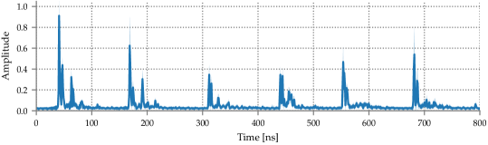
Figure 24. Average CIR amplitude and standard deviation per time delay across 500 signals with the initiator in the left center position of Figure 28.

We begin by examining the ability of our TX compensation mechanism (§5.1) to schedule transmissions precisely, as this is crucial to improve the accuracy of concurrent ranging and localization. To this end, we ran an experiment with one initiator and six responders, collecting 500 CIR signals for our analysis. Figure 24 shows the average CIR amplitude and standard deviation after re-arranging the CIRs (§5.3.1) and aligning the upsampled CIR signals based on the direct path of responder $R_{1}$. Across all time delays, the average CIR presents only minor amplitude variations in the direct paths and MPC. Further, the precise scheduling of response transmissions yields a high amplitude for the direct paths of all signals; this is in contrast with the smoother and flatter peaks we observed earlier (§4, Figure 13) due to the TX uncertainty $\epsilon\in[-8,0)$ ns.

To quantitatively analyze the TX precision, we estimate the ToA of each response and measure the time difference $\Delta t_{j,1}$ between the ToA of responder $R_{j}$ and the one of $R_{1}$, chosen as reference, after removing the time delays $\delta_{i}$ used for response identification. Then, we subtract the mean of the distribution and look at the deviations of $\Delta t_{j,1}$, which ideally should be negligible. Figure 25 shows the CDF of the $\Delta t_{j,1}$ variations from the mean, while Table 4 details the percentiles of the absolute variations. All time differences present a similar behavior with an aggregate mean error $\mu=0.004$ ns across the 2,500 $\Delta t_{j,1}$ measurements, with $\sigma=0.38$ ns and a median of $0.03$ ns; the absolute 90^th, 95^th, and 99^th percentiles are 0.64, 0.77, and 1.09 ns, respectively. These results confirm that our implementation is able to reliably schedule transmissions with sub-ns precision.

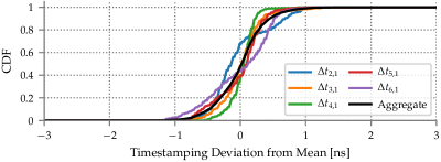
Figure 25. Time difference deviation from the mean across 500 CIRs.

Table 4. Deviation percentiles for the absolute time difference $\Delta t_{j,1}$ variations.

	Percentile [ns]
Time Difference	25th	50th	75th	90th	95th	99th
$\Delta t_{2,1}$	0.15	0.32	0.52	0.72	0.85	1.08
$\Delta t_{3,1}$	0.08	0.18	0.32	0.51	0.68	1.12
$\Delta t_{4,1}$	0.06	0.13	0.20	0.30	0.40	0.60
$\Delta t_{5,1}$	0.13	0.23	0.40	0.64	0.74	0.90
$\Delta t_{6,1}$	0.24	0.39	0.54	0.76	0.91	1.14
Aggregate	0.10	0.23	0.42	0.64	0.77	1.09

6.4. Performance with Static Targets

We report the results from experiments in a $6.4\times 6.4$ m² area inside our office building, using 6 concurrent responders that serve as localization anchors. We place the initiator in 18 different positions and collect 500 CIR signals at each of them, amounting to 9,000 signals.

The choice of initiator positions is key to our analysis. As shown in Figure 28, we split the 18 positions in two halves with different purposes. The 9 positions in the center dashed square are representative of the positions of interest for most applications, as they are farther from walls and enjoy the best coverage w.r.t. responders, when these serve as anchors. Dually, the remaining 9 positions can be regarded as a stress test of sorts. They are very close to walls, yielding significant MPC; this is an issue with conventional SS-TWR but is exacerbated in concurrent ranging, as it increases the possibility to confuse MPC with the direct paths of responders. Further, these positions are at the edge of the area delimited by anchors, therefore yielding a more challenging geometry for localization. Hereafter, we refer to these two sets of positions as center and edge, respectively, and analyze the performance in the common case represented by center as well as in the more challenging, and somewhat less realistic, case where all positions are considered.

In each position, we measure the ranging and localization performance of concurrent ranging with both our ToA estimation algorithms (§5.4.1) and compare it, in the same setup, against the performance of the two SS-TWR variants we consider.

Ranging Accuracy. Figure 26a shows the CDF of the ranging error $\hat{d}_{i}-d_{i}$ obtained with concurrent ranging and SS-TWR in center positions; Table 5 offers an alternate view by reporting the values of the metrics we consider (§6.2).

The performance of concurrent ranging in this setting, arguably the one of interest for most applications, is remarkable and in line with the one of SS-TWR. All variants achieve a similar centimeter-level median and average error. Although SS-TWR exhibits a smaller $\sigma$, both concurrent ranging and SS-TWR achieve decimeter-level precision. This is also reflected in the absolute error, which is nonetheless very small. Both variants of concurrent ranging achieve $99^{\mathit{th}}=28$ cm, only a few cm higher than plain SS-TWR, while its drift compensated variant achieves a lower $99^{\mathit{th}}=18$ cm. The latter SS-TWR variant is the technique that, as expected, achieves the best results across the board. Nevertheless, concurrent ranging measures the distance to the $N=6$ responders concurrently, reducing the number of two-way exchanges from 6 to 1, therefore providing a significant reduction in channel utilization and other evident benefits in terms of latency, energy, and scalability. Interestingly, the difference in accuracy and precision between the two concurrent ranging variants considered is essentially negligible.

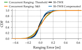
(a) center positions.

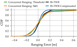
(b) All positions.

Figure 26. CDF of ranging error with static positions.

Table 5. Ranging error comparison across the 9 center positions considered.

	$\hat{d}_{i}-d_{i}$ [cm]			$|\hat{d}_{i}-d_{i}|$ [cm]
Scheme	Median	$\mu$	$\sigma$	50th	75th	90th	95th	99th
Concurrent Ranging: Threshold	0.4	0.3	11.9	8	14	19	21	28
Concurrent Ranging: S&S	0.7	0.5	11.7	7	12	18	21	28
SS-TWR	-1.7	-0.5	8.6	5	9	15	19	22
SS-TWR Compensated	-0.3	-0.3	6.9	4	8	12	14	18

Table 6. Ranging error comparison across the 18 static positions considered (both center and edge).

	$\hat{d}_{i}-d_{i}$ [cm]			$|\hat{d}_{i}-d_{i}|$ [cm]
Scheme	Median	$\mu$	$\sigma$	50th	75th	90th	95th	99th
Concurrent Ranging: Threshold	0.4	2.0	17.7	9	15	21	28	81
Concurrent Ranging: S&S	0.1	3.1	20.4	8	14	23	44	91
SS-TWR	1.5	2.1	8.8	6	10	16	19	23
SS-TWR Compensated	0.4	0.2	6.9	5	8	12	14	18

Figure 26b shows instead the CDF of the ranging error across all positions, i.e., both center and edge, while Table 6 shows the values of the metrics we consider. The difference in accuracy between the two concurrent ranging variants is still negligible in aggregate terms, but slightly worse for S&S when considering the absolute error; this is balanced by a higher reliability w.r.t. the threshold-based variant, as discussed later. In general, the accuracy of concurrent ranging is still comparable to the center case in terms of median and average error, although with slightly worse precision. This is also reflected in the absolute error, which remains very small and essentially the same as in the center case until the $75^{\mathit{th}}$ percentile, but reaches $99^{\mathit{th}}=91$ cm with S&S. In contrast, the performance of both variants of SS-TWR is basically unaltered.

These trends can also be observed in the alternate view of Figure 27, based on normalized histograms. The distributions of concurrent ranging and SS-TWR are similar, although the latter is slightly narrower. Nevertheless, concurrent ranging has a small tail of positive errors, not present in SS-TWR, yielding higher values of $\sigma$ and $\geq 90^{\mathit{th}}$ percentiles in Table 6. Further, these tails are also not present in the case of center, whose distribution is otherwise essentially the same, and therefore not shown due to space limitations.

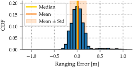
(a) Threshold-based ToA estimation.

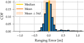
(b) S&S with $K=3$ iterations.

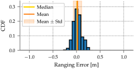
(c) SS-TWR.

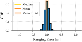
(d) SS-TWR with drift compensation.

Figure 27. Normalized histogram of ranging error across all 18 static positions (both center and edge).

This is to be ascribed to edge positions, in which the initiator i) is next to a wall suffering from closely-spaced and strong MPC next to the direct path, and ii) is very close to one or two anchors and far from the others, resulting in significantly different power loss across responses. This setup sometimes causes the direct path of some responses to be buried in MPC noise or even unable to cross the noise threshold $\eta$. As a result, our ToA algorithms erroneously select one of the MPC peaks as the first path, yielding an incorrect distance estimate. Nevertheless, as mentioned, the absolute error remains definitely acceptable with both the threshold-based and S&S ToA algorithms.

Localization Accuracy. Figure 28 shows the localization error and $3\sigma$ ellipses for each initiator position and both ToA estimation algorithms, while Table 7–8 show the values of the metrics we consider. Coherently with the analysis of ranging accuracy, the standard deviation $\sigma$ for concurrent ranging is significantly lower in the center positions than in the edge ones. This is a consequence of the distance overestimation we observed, which causes larger ellipses and a small bias w.r.t. the true position in a few edge positions. Interestingly, both ToA algorithms underperform in the same positions, although sometimes with different effects, e.g., in positions $(1.6,-3.2)$ and $(3.2,-1.6)$.

The difference between SS-TWR and concurrent ranging is also visible in the longer tails of the localization error CDF (Figure 29b), where it is further exacerbated by the fact that, in our setup, the worst-case edge positions are as many as the common-case center ones. Nevertheless, even in this challenging case, Table 8 shows that concurrent ranging still achieves decimeter-level accuracy, with the median nearly the same as plain SS-TWR. The error is also quite small; $75^{\mathit{th}}\leq 17$ cm and $99^{\mathit{th}}\leq 57$ cm, with the threshold-based approach performing marginally better than S&S, as in ranging. However, the drift compensated SS-TWR is still the most accurate and precise.

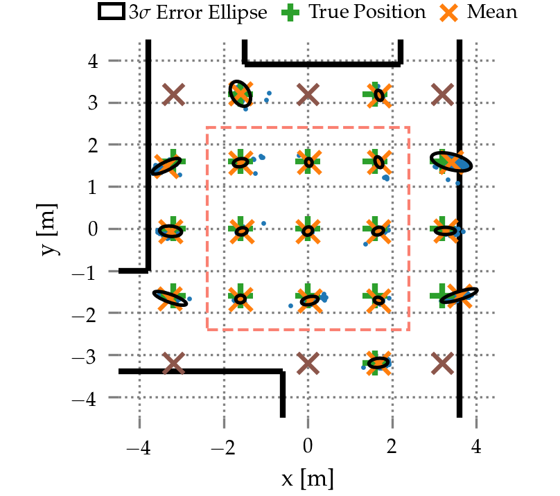
(a) Threshold-based ToA estimation.

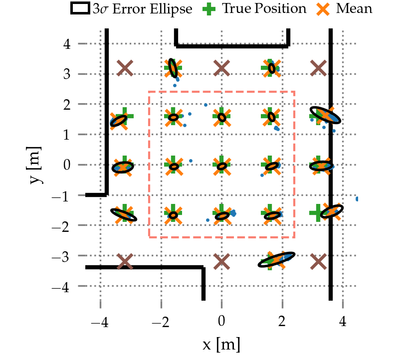
(b) S&S with $K=3$ iterations.

Figure 28. $3\sigma$ error ellipses with concurrent ranging and six concurrent responders. Blue dots represent position estimates, brown crosses are anchors. The dashed light red square denotes the positions of interest.

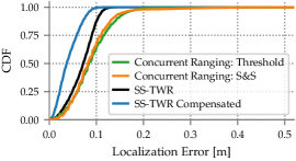
(a) center positions.

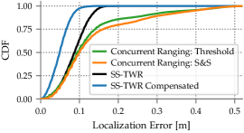
(b) All positions.

Figure 29. CDF of localization error in static positions.

The gap with SS-TWR further reduces in the more common center positions, where the accuracy of concurrent ranging is very high, as shown in Figure 28 and Figure 29a. Position estimates are also quite precise, with $\sigma\leq 5$ cm. Further, the error remains $\leq 16$ cm in $95\%$ of the cases, regardless of the ToA estimation technique; the threshold-based and S&S ToA algorithms show only a marginal difference, with a 99^th percentile of $21$ cm and $30$ cm, respectively.

Table 7. Localization error comparison across the 9 center positions considered.

	$\left\lVert\mathbf{\hat{p}}-\mathbf{p_{r}}\right\rVert$ [cm]
Scheme	$\mu$	$\sigma$	50th	75th	90th	95th	99th
Concurrent Ranging: Threshold	9	4.9	8	12	14	16	21
Concurrent Ranging: S&S	8.8	5	8	11	14	16	30
SS-TWR	6.9	2.7	7	9	10	11	12
SS-TWR Compensated	4.1	2.3	4	6	8	8	10

Table 8. Localization error comparison across the 18 static positions considered (both center and edge).

	$\left\lVert\mathbf{\hat{p}}-\mathbf{p_{r}}\right\rVert$ [cm]
Scheme	$\mu$	$\sigma$	50th	75th	90th	95th	99th
Concurrent Ranging: Threshold	12.9	11	10	14	28	41	51
Concurrent Ranging: S&S	14.5	12.6	10	17	33	42	57
SS-TWR	8.6	3.4	9	11	13	14	16
SS-TWR Compensated	5	2.4	5	7	8	9	11

Success Rate. Across the 9,000 CIR signals considered in this section, concurrent ranging is able to extract a position estimate in 8,663 and 8,973 of them using our threshold-based and S&S ToA estimation, respectively, yielding a remarkable localization success rate of $96.25\%$ and $99.7\%$. Across the successful estimates, 6 samples included very large errors $\geq 10$ m. These could be easily discarded with common filtering techniques (Julier and Uhlmann, 1997). In the center positions of interest, the localization success rate with both ToA techniques yields $99.7\%$.

Threshold-based ToA estimation is more susceptible to strong and late MPC occurring at the beginning of the following CIR chunk, which result in invalid distance estimates that are therefore discarded, reducing the success rate. As for S&S, of the $27$ signals failing to provide an estimate, $21$ are caused by PHR errors where the DW1000 does not update the RX timestamp. In the remaining 6 signals, S&S was unable to detect the first or last responder; these signals were therefore discarded, to avoid a potential responder mis-identification (§5.4.1).

Regarding ranging, threshold-based estimation yields a success rate of $95.98\%$ across the 54,000 expected estimates, while S&S reaches $99.58\%$, in line with the localization success rate.

6.5. Performance with Mobile Targets

We now evaluate the ability of concurrent ranging to accurately determine the position of a mobile node. This scenario is representative of several real-world applications, e.g., exploration in harsh environments (Janicijevic et al., 2018), drone operation (Guo et al., 2016), and user navigation in museums or shopping centers (Yalowitz and Bronnenkant, 2009).

To this end, we ran experiments with an EVB1000 mounted on a mobile robot (did, [n.d.]) in a $12\times 8$ m² indoor area where we placed 6 responders serving as localization anchors. We compare both our concurrent ranging variants against only SS-TWR with clock drift compensation, as this provides a more challenging baseline, as discussed earlier. The area is equipped with 14 OptiTrack cameras (opt, [n.d.]), which we configured to output positioning samples with an update rate of 125 Hz and calibrated to obtain a mean 3D error $<1$ mm, therefore yielding reliable and accurate ground truth to validate the UWB systems against. The mobile robot is controlled by a RPi, enabling us to easily repeat trajectories by remotely driving the robot over WiFi via a Web application on a smartphone. A second RPi enables the flashing of the EVB1000 node with the desired binary and the upload of serial output (CIRs and RX information) to our testbed server for offline analysis.

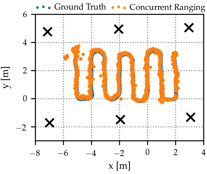
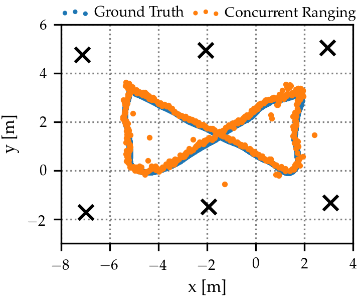
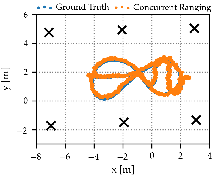
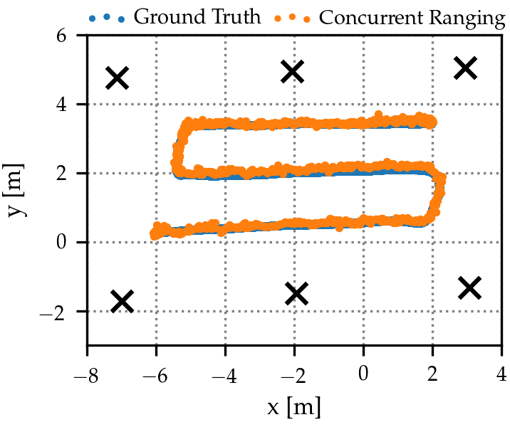
Figure 30. Localization with concurrent ranging across four trajectories using S&S with $K=3$ iterations.

Before presenting in detail our evaluation, Figure 30 offers the opportunity to visually ascertain that our concurrent ranging prototype is able to continuously and accurately track the robot trajectory, by comparing it against the ground truth obtained with OptiTrack. We observe a few position samples with relatively high error, due to strong MPC; however, these situations are rare and, in practice, easily handled with techniques commonly used in position tracking, e.g., extended or unscented Kalman filters (Julier and Uhlmann, 1997). Due to space constraints, the figure shows only trajectories with S&S because they are very similar to threshold-based ones, as discussed next.

Ranging Accuracy. Across all samples, we compute the ranging error $\hat{d}_{i}-d_{i}$ between the concurrent ranging or SS-TWR estimate $\hat{d}_{i}$ for $R_{i}$ and the OptiTrack estimate $d_{i}$. To obtain the latter, we interpolate the high-rate positioning traces of OptiTrack to compute the exact robot position $\mathbf{p}$ at each time instance of our concurrent ranging and SS-TWR traces and then estimate the true distance $d_{i}=\left\lVert\mathbf{p}-\mathbf{p_{i}}\right\rVert$, where $\mathbf{p_{i}}$ is the known position of $R_{i}$.

Table 9 shows that the results exhibit the very good trends we observed in the static case (§6.4). In terms of accuracy, the median and average error are very small, and very close to SS-TWR. However, SS-TWR is significantly more precise, while the standard deviation $\sigma$ of concurrent ranging is in line with the one observed with all 18 positions (Table 6). In contrast, however, the absolute error is $99^{\mathit{th}}\leq 37$ cm, significantly lower than in this latter case. Further, the ToA algorithm employed for concurrent ranging has only a marginal impact on accuracy and precision.

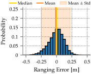
(a) Concurrent ranging: Threshold.

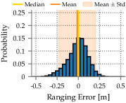
(b) Concurrent ranging: S&S.

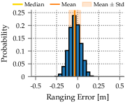
(c) SS-TWR with drift compensation.

Figure 31. Normalized histogram of the ranging error across multiple mobile trajectories.

Table 9. Ranging error comparison across multiple mobile trajectories.

	$\hat{d}_{i}-d_{i}$ [cm]			$|\hat{d}_{i}-d_{i}|$ [cm]
Scheme	Median	$\mu$	$\sigma$	50th	75th	90th	95th	99th
Concurrent Ranging: Threshold	0.3	-1.3	23.5	8	14	20	25	37
Concurrent Ranging: S&S	0.2	-1.4	21.6	8	13	20	24	35
SS-TWR Compensated	-3.5	-3.4	6.8	5	9	12	15	19

An alternate view confirming these observations is offered by the normalized histograms in Figure 31, where the long error tails observed in Figure 27a–27b are absent in Figure 31a–31b.

Overall, concurrent ranging follows closely the performance of SS-TWR with drift compensation, providing a more scalable scheme with less overhead and comparable accuracy. Notably, concurrent ranging measures the distance to all responders simultaneously, an important factor when tracking rapidly-moving targets to reduce the bias induced by relative movements. Further, this aspect also enables a significant increase of the attainable update rate.

Localization Accuracy. Figure 32 compares the CDFs of the localization error of the techniques under evaluation; Table 10 reports the value of the metrics considered. The accuracy of SS-TWR is about 1 cm worse w.r.t. the static case, while the precision is essentially unaltered. As for concurrent ranging, the median error is also the same as in the static case, while the value of the other metrics is by and large in between the case with all positions and the one with only center ones. The precision is closer to the case of all static positions (Table 8), which is mirrored in the slower increase of the CDF for concurrent ranging variants w.r.t. SS-TWR (Figure 32). Overall, the absolute error is relatively small and closer to the case with center positions, with $95^{\mathit{th}}\leq 22$ cm. On the other hand, the 99^th percentile is slightly higher than in Table 8, possibly due to the different environment and the higher impact of the orientation of the antenna relative to the responders. Another difference w.r.t. the static case is the slightly higher precision and 99^th accuracy of S&S vs. threshold-based estimation, in contrast with the opposite trend we observed in §6.4. Again, this is likely to be ascribed to the different environment and MPC profile. In any case, this bears only a minor impact on the aggregate performance, as shown in Figure 32.

Success Rate. Across the 4,015 signals from our trajectories, concurrent ranging obtained 3,999 position estimates ($99.6\%$) with both ToA techniques. Nevertheless, 43 of these are affected by an error $\geq 10$ m and can be disregarded as outliers, yielding an effective success rate of $98.8\%$, which nonetheless reasserts the ability of concurrent ranging to provide reliable and robust localization.

Regarding ranging, threshold-based estimation yields a success rate of $93.18\%$ across the 24,090 expected estimates, while S&S reaches $95.4\%$, confirming its higher reliability. As expected, the localization success rate is higher as the position can be computed even if several $\hat{d}_{i}$ are lost.

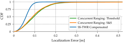
Figure 32. Localization error CDF of concurrent ranging vs. compensated SS-TWR across multiple trajectories.

Table 10. Localization error comparison across multiple mobile trajectories.

	$\left\lVert\mathbf{\hat{p}}-\mathbf{p_{r}}\right\rVert$ [cm]
Scheme	$\mu$	$\sigma$	50th	75th	90th	95th	99th
Concurrent Ranging: Threshold	12.1	17.2	10	14	18	22	85
Concurrent Ranging: S&S	11	12.8	9	13	18	20	60
SS-TWR Compensated	5.8	2.3	6	7	9	10	12

7. Discussion

The outcomes of our evaluation (§6) across several static positions and mobile trajectories in two indoor environments prove that concurrent ranging reliably provides distance and position estimates with decimeter-level accuracy and high precision. The results we presented confirm that concurrent ranging achieves a performance akin to conventional schemes, and that it satisfies the strict requirements of most applications, notably including robot localization.

Nevertheless, concurrent ranging incurs only a small fraction of the cost borne by conventional schemes. SS-TWR requires $2\times N$ packets to measure the distance to $N$ nodes; concurrent ranging achieves the same goal with a single two-way exchange. At the initiator, often a mobile, energy-bound node, only 2 packets need to be TX/RX instead of $2\times N$, proportionally reducing energy consumption and, dually, increasing lifetime. Overall, the ability to perform ranging via shorter exchanges dramatically reduces channel utilization and latency, therefore increasing scalability and update rate. To concretely grasp these claims, consider that, with the (conservative) response delay $T_{\mathit{RESP}}=$800\text{\,}\mathrm{\SIUnitSymbolMicro s}$$ we used, concurrent ranging could provide a location update rate of $\geq$1,000 Hz, either to a single initiator or shared among several ones.

Actually achieving these update rates, however, requires a better hardware and software support than in our prototype. Currently we log the CIR via USB/UART, as it is the only option with the off-the-shelf Decawave EVB1000 boards we use. This choice simplifies our prototyping and enables replication of our results by others, using the same popular and easily available platform. However, it introduces significant delays, reducing the location update rate down to only $\approx$8 Hz; this is appropriate for many applications but insufficient in others requiring the tracking of fast-moving targets, e.g., drones. Nevertheless, this limitation is easily overcome by production systems exploiting more powerful and/or dedicated components, as in the case of smartphones.

Further, this is an issue only if the high update rate theoretically available must be exploited by a single initiator. Otherwise, when shared across several ones, our non-optimized prototype could provide its 8 samples per second to $\approx$125 nodes. This would require a proper scheduling across initiators to avoid collisions, e.g., as in (Kempke et al., 2016a; Vecchia et al., 2019b), and incur overhead, ultimately reducing the final update rate of the system. On the other hand, the potential for collisions is significantly reduced with our technique, given that a single concurrent ranging exchange retrieves the information accrued via $N$ conventional ones. Further, communicating the schedule could itself exploit concurrent transmissions (Kempke et al., 2016a; Lobba et al., 2020; Vecchia et al., 2019a), opening the intriguing possibility of merging scheduling and ranging into a single concurrent exchange abating at once the overhead of both procedures.

Similar issues arise in more dynamic scenarios where ranging is performed against mobile nodes instead of fixed anchors, e.g., to estimate distance between humans as in proxemics applications (Hall, 1966; Greenberg et al., 2011). In cases where the set of nodes is not known a priori, scheduling must be complemented by continuous neighbor discovery, to determine the set of potential ranging targets. The problem of jointly discovering, scheduling, and ranging against nodes has received very little attention by the research community, although it is likely to become important for many applications once UWB becomes readily available on smartphones. In this context, the ability to perform fast and energy-efficient concurrent ranging against several nodes at once brings a unique asset, which may be further enhanced by additional techniques like the adaptive response delays we hinted at in §5.2. The exploration of these and other research avenues enabled by the concurrent ranging techniques we presented in this paper is the subject of our ongoing work.

Finally, the research findings and system prototypes we describe in this paper are derived for the DW1000, i.e., the only UWB transceiver available off-the-shelf today. Nevertheless, new alternatives are surfacing on the market. We argue that the fundamental concept of concurrent ranging and the associated techniques outlined here are of general validity, and therefore in principle transferable to these new transceivers. Moreover, it is our hope that the remarkable benefits we have shown may inspire new UWB architectures that natively support concurrent ranging directly in hardware.

8. Related Work

We place concurrent ranging in the context of other UWB ranging schemes (§8.1), the literature on concurrent transmissions in low-power wireless communications (§8.2), and techniques that build upon the work (Corbalán and Picco, 2018) in which we introduced the notion of concurrent ranging for the first time (§8.3).

8.1. Other UWB Ranging Schemes

Although SS-TWR is a simple and popular scheme for UWB, several others exist, focusing on improving different aspects of its operation.

A key issue is the linear relation between the ranging error and the clock drift (§2.3). Some approaches extend SS-TWR by adding an extra packet from the initiator to the responder (Kempke et al., 2015) or from the responder to the initiator (Mueller et al., 2015). The additional packet enables clock drift compensation.

Instead, double-sided two-way ranging (DS-TWR), also part of the IEEE 802.15.4 standard (std, 2011), includes a third packet from the initiator to the responder in reply to its response, yielding a more accurate distance estimate at the responder; a fourth, optional packet back to the initiator relays the estimate to it. In the classic symmetric scheme (Jiang and Leung, 2007), the response delay $T_{\mathit{RESP}}$ for the response is the same for the third packet from initiator to responder. This constraint reduces flexibility and increases development complexity (Ltd., 2017, p. 225). In the alternative asymmetric scheme proposed by Decawave (McLaughlin and Verso, 2018; Neirynck et al., 2016), instead, the error does not depend on the delays of the two packets; further, the clock drift is reduced to picoseconds, making ToA estimation the main source of error (Ltd., 2017). However, DS-TWR has significantly higher latency and energy consumption, requiring up to $4\times N$ packets (twice than SS-TWR) to measure the distance to $N$ nodes at the initiator. We are currently investigating if and how concurrent ranging can be extended towards DS-TWR.

PolyPoint (Kempke et al., 2015) and SurePoint (Kempke et al., 2016a) improve ranging and localization by using a custom-designed multi-antenna hardware platform. These schemes exploit antenna and channel diversity, yielding more accurate and reliable estimates; however, this comes at the cost of a significantly higher latency and energy consumption, decreasing scalability and battery lifetime.

Other schemes have instead targeted directly a reduction of the packet overhead. The one-way ranging in (Ledergerber et al., 2015) exploits sequential transmissions from anchors to enable mobile nodes to passively self-position, by precisely estimating the time of flight and the clock drift. However, the update rate and accuracy decrease as the number $N$ of anchors increases. Other schemes replace the unicast poll of SS-TWR with a broadcast one, as in concurrent ranging. In N-TWR (Despaux et al., 2018), responders send their response sequentially, to avoid collisions, reducing the number of packets exchanged to $N+1$. An alternate scheme by Decawave (Ltd., 2017, p. 227) exploits a broadcast poll in asymmetric DS-TWR, rather than SS-TWR, reducing the packet overhead to $2+N$ or $2(N+1)$ depending on whether estimates are obtained at the responders or the initiator, respectively.

In all these schemes, however, the number of packets required grows linearly with $N$, limiting scalability. In contrast, concurrent ranging measures the distance to the $N$ nodes based on a single two-way exchange, reducing dramatically latency, consumption, and channel utilization, yet providing similar accuracy as demonstrated in §6.

8.2. Concurrent Transmissions for Low-power Wireless Communication

Our concurrent ranging technique was originally inspired by the body of work on concurrent transmissions in narrowband low-power radios. Pioneered by Glossy (Ferrari et al., 2011), this technique exploits the PHY-level phenomena of constructive interference and capture effect to achieve unprecedented degrees of high reliability, low latency, and low energy consumption, as shown by several follow-up works (Landsiedel et al., 2013; Ferrari et al., 2012; Istomin et al., 2016). However, these focus on IEEE 802.15.4 narrowband radios, leaving an open question about whether similar benefits can be harvested for UWB radios.

In (Vecchia et al., 2019a) we ascertained empirically the conditions for exploiting UWB concurrent transmissions for reliable communication, exploring extensively the radio configuration space. The findings serve as a foundation for adapting the knowledge and systems in narrowband towards UWB and reaping similar benefits, as already exemplified by (Lobba et al., 2020). Further, the work in (Vecchia et al., 2019a) also examined the effect of concurrent transmissions on ranging—a peculiarity of UWB not present in narrowband—confirming our original findings in (Corbalán and Picco, 2018) (and §4) and analyzing the radio configuration and environmental conditions in more depth and breadth than what we can report here.

8.3. Concurrent Transmissions for Ranging and Localization

We introduced the novel concept of concurrent ranging in (Corbalán and Picco, 2018), where we demonstrated the feasibility of exploiting UWB concurrent transmissions together with CIR information for ranging; §4 contains an adapted account of the observations we originally derived. Our work was followed by (Großwindhager et al., 2018), which introduces the idea of using pulse shapes and response position modulation to match CIR paths with responders. We discarded the former in §5.2 and (Corbalán et al., 2019) as we verified empirically that closely-spaced MPC can create ambiguity, and therefore mis-identifications. Here, we resort to the latter as in (Corbalán et al., 2019; Großwindhager et al., 2019), i.e., by adding a small time shift $\delta_{i}$ to each response, enough to separate the signals of each responder throughout the CIR span. The work in (Großwindhager et al., 2018) also suggested a simpler version of Search & Subtract for ToA estimation. Instead, here we follow the original algorithm (Falsi et al., 2006) but enforce that candidate paths reach a minimum peak amplitude, to improve resilience to noise and MPC. Moreover, we introduce an alternate threshold-based ToA algorithm that is significantly simpler but yields similar results. Both preliminary works in (Corbalán and Picco, 2018; Großwindhager et al., 2018) leave as open challenges the TX scheduling uncertainty and the unreliability caused by packet loss. Here, we address these challenges with the local compensation mechanism in §5.1 and the other techniques in §5, making concurrent ranging not only accurate, but also very reliable and, ultimately, usable in practice.

Decawave (McLaughlin and J., 2019) filed a patent on “simultaneous ranging” roughly at the same time of our original work (Corbalán and Picco, 2018), similarly exploiting concurrent transmissions from responders. The patent includes two variants: i) a parallel version, where all responders transmit nearly simultaneously as in §3–§4, only aiming to measure the distance to the closest responder, and ii) a staggered version that exploits time shifts as in §5.2 to determine the distance to each responder. The latter, however, requires PHY-layer changes that will unavoidably take time to be standardized and adopted by future UWB transceivers. In contrast, the techniques we present here can be exploited with current transceivers and can also serve as a reference for the design and development of forthcoming UWB radios natively supporting concurrent ranging.

Our original paper inspired follow-up work on concurrent ranging (Großwindhager et al., 2018; Heydariaan et al., 2019) but also on other techniques exploiting concurrent transmissions for localization. Our own Chorus (Corbalán et al., 2019) system and SnapLoc (Großwindhager et al., 2019) realize a passive self-localization scheme supporting unlimited targets. Both systems assume a known anchor infrastructure in which a reference anchor transmits a first packet to which the others reply concurrently. Mobile nodes in range listen for these concurrent responses and estimate their own position based on time-difference of arrival (TDoA) multilateration. In (Corbalán et al., 2019), we modeled the accuracy of estimation via concurrent transmissions if the TX uncertainty were to be reduced, as expected in forthcoming UWB transceivers. This model is applicable to concurrent ranging and, in fact, predicts the results we achieved in §6 by locally compensating for the TX uncertainty (§5.1). SnapLoc instead proposed to directly address the TX uncertainty with a correction that requires either a wired backbone infrastructure that anchors exploit to report their known TX error, or a reference anchor that receives the response and measures each TX error from the CIR. Both require an additional step to report the error to mobile nodes, and introduce complexity in the deployment along with communication overhead. In contrast, the compensation in §5.1 is entirely local to the responders, therefore imposing neither deployment constraints nor overhead. Moreover, the compensation in §5.1 can be directly incorporated in Chorus and SnapLoc, improving their performance while simplifying their designs.

Recently, these works have also inspired the use of UWB concurrent transmissions with angle-of-arrival (AoA) localization. In (Wang et al., 2020), a multi-antenna anchor sends a poll to which mobile nodes in range reply concurrently, allowing the anchor not only to measure their distance but also the AoA of their signals; combining the two enables the anchor to estimate the position of each node. The techniques we proposed in this paper (§5) addressing the TX uncertainty, clock drift, and unreliability caused by packet loss, are applicable and likely beneficial also for this AoA technique.

9. Conclusions

In (Corbalán and Picco, 2018), we described the novel concept of concurrent ranging for the first time in the literature, demonstrated its feasibility, elicited the open challenges, and outlined the several benefits it could potentially enable in terms of latency, scalability, update rate, and energy consumption.

In this paper, we make these benefits a tangible reality. We tackle the aforementioned challenges with a repertoire of techniques that, without requiring modifications to off-the-shelf UWB transceivers, turn concurrent ranging into a practical and immediately available approach. Concurrent ranging empowers the designers of UWB ranging and localization systems with a new option whose accuracy is comparable to conventional techniques, but comes at a fraction of the latency and energy costs, therefore unlocking application trade-offs hitherto unavailable for these systems.

- (1)
- did ([n.d.]) [n.d.]. DiddyBorg v2 Robot Kit. Online: https://www.piborg.org/robots-1/diddyborg-v2, last accessed on 08/01/2020.
- opt ([n.d.]) [n.d.]. OptiTrack. Online: https://optitrack.com/motion-capture-robotics/, last accessed on 08/01/2020.
- vic ([n.d.]) [n.d.]. Vicon. Online: https://www.vicon.com, last accessed on 22/01/2020.
- std (2011) 2011. IEEE Standard for Local and metropolitan area networks–Part 15.4: Low-Rate Wireless Personal Area Networks (LR-WPANs).
- Benini et al. (2013) A. Benini, A. Mancini, and S. Longhi. 2013. An IMU/UWB/Vision-based Extended Kalman Filter for Mini-UAV Localization in Indoor Environment using 802.15.4a Wireless Sensor Network. Journal of Intelligent & Robotic Systems 70, 1-4 (2013), 461–476.
- Branch et al. (1999) M. A. Branch, T. F. Coleman, and Y. Li. 1999. A Subspace, Interior, and Conjugate Gradient Method for Large-Scale Bound-Constrained Minimization Problems. SIAM Journal on Scientific Computing 21, 1 (1999), 1–23.
- Corbalán et al. (2018) P. Corbalán, T. Istomin, and G. P. Picco. 2018. Poster: Enabling Contiki on Ultra-wideband Radios. In Proc. of the 15th Int. Conf. on Embedded Wireless Systems and Networks (EWSN).
- Corbalán and Picco (2018) P. Corbalán and G. P. Picco. 2018. Concurrent Ranging in Ultra-wideband Radios: Experimental Evidence, Challenges, and Opportunities. In Proc. of the 15th Int. Conf. on Embedded Wireless Systems and Networks (EWSN).
- Corbalán et al. (2019) P. Corbalán, G. P. Picco, and S. Palipana. 2019. Chorus: UWB Concurrent Transmissions for GPS-like Passive Localization of Countless Targets. In Proc. of the 18th Int. Conf. on Information Processing in Sensor Networks (IPSN).
- Despaux et al. (2018) F. Despaux, A. van den Bossche, K. Jaffrès-Runser, and T. Val. 2018. N-TWR: An accurate time-of-flight-based N-ary ranging protocol for Ultra-Wide band. Ad Hoc Networks 79 (oct 2018), 1–19.
- Domain (2011) Time Domain. 2011. Time Domain PulsON 400 RCM Data Sheet.
- Dotlic et al. (2018) I. Dotlic, A. Connell, and M. McLaughlin. 2018. Ranging Methods Utilizing Carrier Frequency Offset Estimation. In Proc. of the 15th Workshop on Positioning, Navigation and Communications (WPNC).
- Falsi et al. (2006) C. Falsi, D. Dardari, L. Mucchi, and M. Z. Win. 2006. Time of Arrival Estimation for UWB Localizers in Realistic Environments. EURASIP J. on Advances in Signal Processing 2006, 1 (2006), 032–082.
- Fenwick (1999) A. J. Fenwick. 1999. Algorithms for position fixing using pulse arrival times. IEE Proceedings–Radar, Sonar and Navigation 146, 4 (1999), 208–212.
- Ferrari et al. (2012) F. Ferrari, M. Zimmerling, L. Mottola, and L. Thiele. 2012. Low-Power Wireless Bus. In Proc. of the 10th ACM Conf. on Embedded Network Sensor Systems (SenSys).
- Ferrari et al. (2011) F. Ferrari, M. Zimmerling, L. Thiele, and O. Saukh. 2011. Efficient Network Flooding and Time Synchronization with Glossy. In Proc. of the 10th Int. Conf. on Information Processing in Sensor Networks (IPSN).
- Fontana et al. (2003) R. J. Fontana, E. Richley, and J. Barney. 2003. Commercialization of an ultra wideband precision asset location system. In Proc. of the IEEE Conf. on Ultra Wideband Systems and Technologies.
- Greenberg et al. (2011) S. Greenberg, N. Marquardt, T. Ballendat, R. Diaz-Marino, and M. Wang. 2011. Proxemic Interactions: The New Ubicomp? interactions 18, 1 (jan 2011), 42–50.
- Großwindhager et al. (2019) B. Großwindhager et al. 2019. SnapLoc: An Ultra-Fast UWB-Based Indoor Localization System for an Unlimited Number of Tags. In Proc. of the 18th Int. Conf. on Information Processing in Sensor Networks (IPSN).
- Großwindhager et al. (2018) B. Großwindhager, C. A. Boano, M. Rath, and K. Römer. 2018. Concurrent Ranging with Ultra-Wideband Radios: From Experimental Evidence to a Practical Solution. In Proc. of the 38th Int. Conf. on Distributed Computing Systems (ICDCS).
- Guo et al. (2016) K. Guo, Z. Qiu, C. Miao, A. H. Zaini, C. L. Chen, W. Meng, and L. Xie. 2016. Ultra-Wideband-Based Localization for Quadcopter Navigation. Unmanned Systems 4, 01 (2016), 23–34.
- Hall (1966) E. T. Hall. 1966. The Hidden Dimension. Doubleday, New York.
- Halperin et al. (2010) D. Halperin, B. Greenstein, A. Sheth, and D. Wetherall. 2010. Demystifying 802.11N Power Consumption. In Proc. of the Int. Conf. on Power Aware Computing and Systems (HotPower).
- Hartmann et al. (2015) F. Hartmann et al. 2015. Design of an Embedded UWB Hardware Platform for Navigation in GPS Denied Environments. In Proc. of the IEEE Symposium on Communications and Vehicular Technology in the Benelux (SCVT).
- Heydariaan et al. (2019) M. Heydariaan, H. Mohammadmoradi, and O. Gnawali. 2019. R3: Reflection Resilient Concurrent Ranging with Ultra-Wideband Radios. In Proc. of the 15th Int. Conf. on Distributed Computing in Sensor Systems (DCOSS).
- Instruments (2016) Texas Instruments. 2016. CC2650 SimpleLinkTM Multistandard Wireless MCU.
- Istomin et al. (2016) T. Istomin, A. L. Murphy, G. P. Picco, and U. Raza. 2016. Data Prediction + Synchronous Transmissions = Ultra-low Power Wireless Sensor Networks. In Proc. of the 14th ACM Conf. on Embedded Network Sensor Systems (SenSys).
- Janicijevic et al. (2018) N. Janicijevic et al. 2018. Demo: Small PLaNS Towards Mars: Exploiting Ultra-wideband for Self-localizing Rover Navigation. In Proc. of the 15th Int. Conf. on Embedded Wireless Systems and Networks (EWSN).
- Jiang and Leung (2007) Y. Jiang and V. C. M. Leung. 2007. An Asymmetric Double Sided Two-Way Ranging for Crystal Offset. In Proc. of the IEEE Int. Symposium on Signals, Systems and Electronics (ISSSE).
- Julier and Uhlmann (1997) S. J. Julier and J. K. Uhlmann. 1997. A New Extension of the Kalman Filter to Nonlinear Systems. In Signal processing, sensor fusion, and target recognition VI, Vol. 3068. International Society for Optics and Photonics, 182–193.
- Kempke et al. (2016a) B. Kempke et al. 2016a. SurePoint: Exploiting Ultra Wideband Flooding and Diversity to Provide Robust, Scalable, High-Fidelity Indoor Localization. In Proc. of the 14th ACM Conf. on Embedded Network Sensor Systems (SenSys).
- Kempke et al. (2015) B. Kempke, P. Pannuto, and P. Dutta. 2015. PolyPoint: Guiding Indoor Quadrotors with Ultra-Wideband Localization. In Proc. of the 2nd Int. Workshop on Hot Topics in Wireless (HotWireless).
- Kempke et al. (2016b) B. Kempke, P. Pannuto, and P. Dutta. 2016b. Harmonium: Asymmetric, Bandstitched UWB for Fast, Accurate, and Robust Indoor Localization. In Proc. of the 15th Int. Conf. on Information Processing in Sensor Networks (IPSN).
- Landsiedel et al. (2013) O. Landsiedel, F. Ferrari, and M. Zimmerling. 2013. Chaos: Versatile and Efficient All-to-all Data Sharing and In-network Processing at Scale. In Proc. of the 11th ACM Conf. on Embedded Networked Sensor Systems (SenSys).
- Lazik et al. (2015) P. Lazik, N. Rajagopal, O. Shih, B. Sinopoli, and A. Rowe. 2015. ALPS: A Bluetooth and Ultrasound Platform for Mapping and Localization. In Proc. of the 13th ACM Conf. on Embedded Networked Sensor Systems (SenSys).
- Lazik and Rowe (2012) P. Lazik and A. Rowe. 2012. Indoor Pseudo-Ranging of Mobile Devices Using Ultrasonic Chirps. In Proc. of the 10th ACM Conf. on Embedded Network Sensor Systems (SenSys ’12). 99–112.
- Ledergerber et al. (2015) A. Ledergerber, M. Hamer, and R. D’Andrea. 2015. A Robot Self-Localization System using One-Way Ultra-Wideband Communication. In Proc. of the IEEE/RSJ Int. Conf. on Intelligent Robots and Systems (IROS).
- Lobba et al. (2020) D. Lobba et al. 2020. Concurrent Transmissions for Multi-hop Communication on Ultra-wideband Radios. In Proc. of the 17th Int. Conf. on Embedded Wireless Systems and Networks (EWSN).
- Ltd. (2013) Decawave Ltd. 2013. Decawave ScenSor EVB1000 Evaluation Board.
- Ltd. (2014) Decawave Ltd. 2014. APS011 Application Note: Sources of Error in DW1000 based Two-way Ranging (TWR) Schemes.
- Ltd. (2016a) Decawave Ltd. 2016a. DW1000 Data Sheet.
- Ltd. (2016b) Decawave Ltd. 2016b. DW1000 Device Driver Application Programming Interface (API) Guide.
- Ltd. (2017) Decawave Ltd. 2017. DW1000 User Manual.
- Ltd. (2018) Decawave Ltd. 2018. APS014 Application Note: Antenna Delay Calibration of DW1000-based products and systems.
- Mao et al. (2017) W. Mao, Z. Zhang, L. Qiu, J. He, Y. Cui, and S. Yun. 2017. Indoor Follow Me Drone. In Proc. of the 15th Annual Int. Conf. on Mobile Systems, Applications, and Services (MobiSys).
- Mattaboni (1987) P. J. Mattaboni. 1987. Autonomous mobile robot. US Patent 4,638,445.
- McLaughlin and J. (2019) M. McLaughlin and Niewczas J. 2019. Ranging with Simultaneous Frames. Patent WO 2019/110833 A1.
- McLaughlin and Verso (2018) M. McLaughlin and B. Verso. 2018. Asymmetric double-sided two-way ranging in an ultrawideband communication system. US Patent App. 15/500,633.
- Molisch et al. (2004) A. F. Molisch et al. 2004. IEEE 802.15. 4a channel model—final report. IEEE P802 15, 04 (2004), 0662.
- Mueller et al. (2015) M. W. Mueller, M. Hamer, and R. D’Andrea. 2015. Fusing ultra-wideband range measurements with accelerometers and rate gyroscopes for quadrocopter state estimation. In Proc. of the IEEE Int. Conf. on Robotics and Automation (ICRA).
- Neirynck et al. (2016) D. Neirynck, E. Luk, and M. McLaughlin. 2016. An Alternative Double-Sided Two-Way Ranging Method. In Proc. of the 13th IEEE workshop on positioning, navigation and communications (WPNC).
- Priyantha et al. (2000) N. B. Priyantha, A. Chakraborty, and H. Balakrishnan. 2000. The Cricket Location-Support System. In Proc. of the 6th Annual Int. Conf. on Mobile Computing and Networking (MobiCom).
- Sandin et al. (2015) P. E. Sandin et al. 2015. Lawn care robot. US Patent 9,043,952.
- So (2011) H. C. So. 2011. Source Localization: Algorithms and Analysis. John Wiley & Sons, Ltd, Chapter 2, 25–66.
- Texas Instruments ([n.d.]) Texas Instruments. [n.d.]. CC2420 Datasheet.
- Tiemann et al. (2016) J. Tiemann, F. Eckermann, and C. Wietfeld. 2016. ATLAS - An Open-Source TDOA-based Ultra-Wideband Localization System. In Proc. of the Int. Conf. on Indoor Positioning and Indoor Navigation (IPIN).
- Vecchia et al. (2019a) D. Vecchia, P. Corbalán, T. Istomin, and G. P. Picco. 2019a. Playing with Fire: Exploring Concurrent Transmissions in Ultra-wideband Radios. In Proc. of the 18th IEEE Int. Conf. on Sensing, Communication and Networking (SECON).
- Vecchia et al. (2019b) D. Vecchia, P. Corbalán, T. Istomin, and G. P. Picco. 2019b. TALLA: Large-scale TDoA Localization with Ultra-wideband Radios. In Proc. of the 10th Int. Conf. on Indoor Positioning and Indoor Navigation (IPIN).
- Wan and Van Der Merwe (2000) E. A. Wan and R. Van Der Merwe. 2000. The unscented Kalman filter for nonlinear estimation. In Proc. of the IEEE Adaptive Systems for Signal Processing, Communications, and Control Symposium (Cat. No.00EX373). 153–158.
- Wang et al. (2020) T. Wang, H. Zhao, and Y. Shen. 2020. An Efficient Single-Anchor Localization Method Using Ultra-Wide Bandwidth Systems. Applied Sciences 10, 1 (2020), 57.
- Win and Scholtz (1998) M. Z. Win and R. A. Scholtz. 1998. Impulse radio: How it works. IEEE Comm. Lett. 2, 2 (1998), 36–38.
- Win and Scholtz (2000) M. Z. Win and R. A. Scholtz. 2000. Ultra-Wide Bandwidth Time-Hopping Spread-Spectrum Impulse Radio for Wireless Multiple-Access Communications. IEEE Transactions on Communications 48, 4 (2000), 679–689.
- Yalowitz and Bronnenkant (2009) S. S. Yalowitz and K. Bronnenkant. 2009. Timing and tracking: Unlocking visitor behavior. Visitor Studies 12, 1 (2009), 47–64.
- Yang and Giannakis (2004) L. Yang and G. B. Giannakis. 2004. Ultra-wideband Communications: An Idea Whose Time Has Come. IEEE Signal Processing 21, 6 (2004), 26–54.